Approximate Newton-based statistical inference
using only stochastic gradients
 

Abstract

We present a novel statistical inference framework for convex empirical risk minimization, using approximate stochastic Newton steps. The proposed algorithm is based on the notion of finite differences and allows the approximation of a Hessian-vector product from first-order information. In theory, our method efficiently computes the statistical error covariance in $M$-estimation, both for unregularized convex learning problems and high-dimensional LASSO regression, without using exact second order information, or resampling the entire data set. We also present a stochastic gradient sampling scheme for statistical inference in non-i.i.d. time series analysis, where we sample contiguous blocks of indices. In practice, we demonstrate the effectiveness of our framework on large-scale machine learning problems, that go even beyond convexity: as a highlight, our work can be used to detect certain adversarial attacks on neural networks.

1 Introduction

Statistical inference is an important tool for assessing uncertainties, both for estimation and prediction purposes [FHT01, EH16]. E.g., in unregularized linear regression and high-dimensional LASSO settings [vdGBRD14, JM15, TWH15], we are interested in computing coordinate-wise confidence intervals and p-values of a $p$-dimensional variable, in order to infer which coordinates are active or not [Was13]. Traditionally, the inverse Fisher information matrix [Edg08] contains the answer to such inference questions; however it requires storing and computing a $p\times p$ matrix structure, often prohibitive for large-scale applications [TRVB06]. Alternatively, the Bootstrap method is a popular statistical inference algorithm, where we solve an optimization problem per dataset replicate, but can be expensive for large data sets [KTSJ14].

While optimization is mostly used for point estimates, recently it is also used as a means for statistical inference in large scale machine learning [LLKC18, CLTZ16, SZ18, FXY17]. This manuscript follows this path: we propose an inference framework that uses stochastic gradients to approximate second-order, Newton steps. This is enabled by the fact that we only need to compute Hessian-vector products; in math, this can be approximated using $\nabla^{2}f(\theta)v\approx\tfrac{\nabla f(\theta+\delta v)-\nabla f(\theta)}{\delta}$, where $f$ is the objective function, and $\nabla f$, $\nabla^{2}f$ denote the gradient and Hessian of $f$. Our method can be interpreted as a generalization of the SVRG approach in optimization [JZ13] (Appendix E); further, it is related to other stochastic Newton methods (e.g. [ABH17]) when $\delta\to 0$. We defer the reader to Section 6 for more details. In this work, we apply our algorithm to unregularized $M$-estimation, and we use a similar approach, with proximal approximate Newton steps, in high-dimensional linear regression.

Our contributions can be summarized as follows; a more detailed discussion is deferred to Section 6:

• For the case of unregularized $M$-estimation, our method efficiently computes the statistical error covariance, useful for confidence intervals and p-values. Compared to state of the art, our scheme $\boldsymbol{(i)}$ guarantees consistency of computing the statistical error covariance, $\boldsymbol{(ii)}$ exploits better the available information (without wasting computational resources to compute quantities that are thereafter discarded), and $\boldsymbol{(iii)}$ converges to the optimum (without swaying around it).

• For high-dimensional linear regression, we propose a different estimator (see (13)) than the current literature. It is the result of a different optimization problem that is strongly convex with high probability. This permits the use of linearly convergent proximal algorithms [XZ14, LSS14] towards the optimum; in contrast, state of the art only guarantees convergence to a neighborhood of the LASSO solution within statistical error. Our model also does not assume that absolute values of the true parameter’s non-zero entries are lower bounded.

• For statistical inference in non-i.i.d. time series analysis, we sample contiguous blocks of indices (instead of uniformly sampling) to compute stochastic gradients. This is similar to the Newey-West estimator [NW86] for HAC (heteroskedasticity and autocorrelation consistent) covariance estimation, but does not waste computational resources to compute the entire matrix.

• The effectiveness of our framework goes even beyond convexity. As a highlight, we show that our work can be used to detect certain adversarial attacks on neural networks.

2 Unregularized $M$-estimation

In unregularized, low-dimensional $M$-estimation problems, we estimate a parameter of interest:

$$\theta^{\star}=\arg\min_{\theta\in\mathbb{R}^{p}}{\operatorname{\mathbb{E}}}_{X\sim P}\left[\ell(X;\theta)\right],\quad\text{where $P(X)$ is the data distribution},$$

using empirical risk minimization (ERM) on $n>p$ i.i.d. data points $\{X_{i}\}_{i=1}^{n}$:

$$\widehat{\theta}=\arg\min_{\theta\in\mathbb{R}^{p}}\tfrac{1}{n}\sum_{i=1}^{n}\ell(X_{i};\theta).$$

Statistical inference, such as computing one-dimensional confidence intervals, gives us information beyond the point estimate $\widehat{\theta}$, when $\widehat{\theta}$ has an asymptotic limit distribution [Was13]. E.g., under regularity conditions, the $M$-estimator satisfies asymptotic normality [vdV98, Theorem 5.21]. I.e., $\sqrt{n}(\widehat{\theta}-\theta^{\star})$ weakly converges to a normal distribution:

$$\sqrt{n}\left(\widehat{\theta}-\theta^{\star}\right)\to\mathcal{N}\left(0,{H^{\star}}^{-1}G^{\star}{H^{\star}}^{-1}\right),$$

where $H^{\star}={\operatorname{\mathbb{E}}}_{X\sim P}[\nabla^{2}_{\theta}\ell(X;\theta^{\star})]$ and $G^{\star}={\operatorname{\mathbb{E}}}_{X\sim P}[\nabla_{\theta}\ell(X;\theta^{\star})\,\nabla_{\theta}\ell(X;\theta^{\star})^{\top}]$. We can perform statistical inference when we have a good estimate of ${H^{\star}}^{-1}G^{\star}{H^{\star}}^{-1}$. In this work, we use the plug-in covariance estimator $\widehat{H}^{-1}\widehat{G}\widehat{H}^{-1}$ for ${H^{\star}}^{-1}G^{\star}{H^{\star}}^{-1}$, where:

$$\widehat{H}=\tfrac{1}{n}\sum_{i=1}^{n}\nabla^{2}_{\theta}\ell(X_{i};\widehat{\theta}),\quad\text{ and }\quad\widehat{G}=\tfrac{1}{n}\sum_{i=1}^{n}\nabla_{\theta}\ell(X_{i};\widehat{\theta})\,\nabla_{\theta}\ell(X_{i};\widehat{\theta})^{\top}.$$

Observe that, in the naive case of directly computing $\widehat{G}$ and $\widehat{H}^{-1}$, we require both high computational- and space-complexity. Here, instead, we utilize approximate stochastic Newton motions from first order information to compute the quantity $\widehat{H}^{-1}\widehat{G}\widehat{H}^{-1}$.

2.1 Statistical inference with approximate Newton steps using only stochastic gradients

Based on the above, we are interested in solving the following $p$-dimensional optimization problem:

$$\widehat{\theta}=\arg\min_{\theta\in\mathbb{R}^{p}}f(\theta):=\tfrac{1}{n}\sum_{i=1}^{n}f_{i}(\theta),\quad\text{where $f_{i}(\theta)=\ell(X_{i};\theta)$.}$$

Notice that $\widehat{H}^{-1}\widehat{G}\widehat{H}^{-1}$ can be written as $\frac{1}{n}$ $\sum_{i=1}^{n}$ $\left(\widehat{H}^{-1}\nabla_{\theta}\ell(X_{i};\widehat{\theta})\right)$ $\left(\widehat{H}^{-1}\nabla_{\theta}\ell(X_{i};\widehat{\theta})\right)^{\top}$, which can be interpreted as the covariance of stochastic –inverse-Hessian conditioned– gradients at $\widehat{\theta}$. Thus, the covariance of stochastic Newton steps can be used for statistical inference.

1:  Parameters: $S_{o},S_{i}\in\mathbb{Z}_{+}$; $\rho_{0},\tau_{0}\in\mathbb{R}_{+}$; $d_{o},d_{i}\in\left(\tfrac{1}{2},1\right)$  Initial state: $\theta_{0}\in\mathbb{R}^{p}$  

2:  for $t=0\text{ to }T-1$ do  // approximate stochastic Newton descent

3:     $\rho_{t}\leftarrow\rho_{0}(t+1)^{-d_{o}}$

4:     $I_{o}\leftarrow$ uniformly sample $S_{o}$ indices with replacement from $[n]$

5:     $g^{0}_{t}\leftarrow-\rho_{t}\left(\frac{1}{S_{o}}\sum_{i\in I_{o}}\nabla f_{i}(\theta_{t})\right)$

6:     for $j=0\text{ to }L-1$ do  // solving (1) approximately using SGD

7:        $\tau_{j}\leftarrow\tau_{0}(j+1)^{-d_{i}}$ and $\delta_{t}^{j}\leftarrow O(\rho_{t}^{4}\tau_{j}^{4})$

8:        $I_{i}\leftarrow$ uniformly sample $S_{i}$ indices without replacement from $[n]$

9:        $g^{j+1}_{t}\leftarrow g_{t}^{j}-\tau_{j}\left(\frac{1}{S_{i}}\sum_{k\in I_{i}}\tfrac{\nabla f_{k}(\theta_{t}+{\delta_{t}^{j}}g_{t}^{j})-\nabla f_{k}(\theta_{t})}{\delta_{t}^{j}}\right)+\tau_{j}g_{t}^{0}$

10:     end for

11:     Use $\sqrt{S_{o}}\cdot\frac{\bar{g}_{t}}{\rho_{t}}$ for statistical inference, where $\bar{g}_{t}=\frac{1}{L+1}\sum_{j=0}^{L}g^{j}_{t}$

12:     $\theta_{t+1}\leftarrow\theta_{t}+g_{t}^{L}$

13:  end for

Algorithm 1 Unregularized M-estimation statistical inference

Algorithm 1 approximates each stochastic Newton $\widehat{H}^{-1}\nabla_{\theta}\ell(X_{i};\widehat{\theta})$ step using only first order information. We start from $\theta_{0}$ which is sufficiently close to $\widehat{\theta}$, which can be effectively achieved using SVRG [JZ13]; a description of the SVRG algorithm can be found in Appendix E. Lines 4, 5 compute a stochastic gradient whose covariance is used as part of statistical inference. Lines 6 to 12 use SGD to solve the Newton step,

$$\min_{g\in\mathbb{R}^{p}}\left\langle\tfrac{1}{S_{o}}\sum_{i\in I_{o}}\nabla f_{i}(\theta_{t}),g\right\rangle+\tfrac{1}{2\rho_{t}}\left\langle g,\nabla^{2}f(\theta_{t})g\right\rangle,$$ (1)

which can be seen as a generalization of SVRG; this relationship is described in more detail in Appendix E. In particular, these lines correspond to solving (1) using SGD by uniformly sampling a random $f_{i}$, and approximating:

$$\nabla^{2}f(\theta)g\approx\tfrac{\nabla f(\theta+{\delta_{t}^{j}}g)-\nabla f(\theta)}{\delta_{t}^{j}}={\operatorname{\mathbb{E}}}\left[\tfrac{\nabla f_{i}(\theta+{\delta_{t}^{j}}g)-\nabla f_{i}(\theta)}{\delta_{t}^{j}}\mid\theta\right].$$ (2)

Finally, the outer loop (lines 2 to 13) can be viewed as solving inverse Hessian conditioned stochastic gradient descent, similar to stochastic natural gradient descent [Ama98].

In terms of parameters, similar to [PJ92, Rup88], we use a decaying step size in Line 8 to control the error of approximating $H^{-1}g$. We set $\delta_{t}^{j}=O(\rho_{t}^{4}\tau_{j}^{4})$ to control the error of approximating Hessian vector product using a finite difference of gradients, so that it is smaller than the error of approximating $H^{-1}g$ using stochastic approximation. For similar reasons, we use a decaying step size in the outer loop to control the optimization error.

The following theorem characterizes the behavior of Algorithm 1.

Theorem 1.

For a twice continuously differentiable and convex function $f(\theta)=\frac{1}{n}\sum_{i=1}^{n}f_{i}(\theta)$ where each $f_{i}$ is also convex and twice continuously differentiable, assume $f$ satisfies

• strong convexity: $\forall\theta_{1},\theta_{2}$, $f(\theta_{2})\geq f(\theta_{1})+\langle\nabla f(\theta_{1}),\theta_{2}-\theta_{1}\rangle+\frac{1}{2}\alpha\|\theta_{2}-\theta_{1}\|_{2}^{2}$;

• $\forall\theta$, each $\|\nabla^{2}f_{i}(\theta)\|_{2}\leq\beta_{i}$, which implies that $f_{i}$ has Lipschitz gradient: $\forall\theta_{1},\theta_{2}$, $\|\nabla f_{i}(\theta_{1})-\nabla f_{i}(\theta_{2})\|_{2}\leq\beta_{i}\|\theta_{1}-\theta_{2}\|_{2}$;

• each $\nabla^{2}f_{i}$ is Lipschitz continuous: $\forall\theta_{1},\theta_{2}$, $\|\nabla^{2}f_{i}(\theta_{2})-\nabla^{2}f_{i}(\theta_{1})\|_{2}\leq h_{i}\|\theta_{2}-\theta_{1}\|_{2}$.

In Algorithm 1, we assume that batch sizes $S_{o}$—in the outer loop—and $S_{i}$—in the inner loops—are $O(1)$. The outer loop step size is

$$\rho_{t}=\rho_{0}\cdot(t+1)^{-d_{o}},\quad\text{where $d_{o}\in\left(\tfrac{1}{2},1\right)$ is the decaying rate. }$$ (3)

In each outer loop, the inner loop step size is

$$\tau_{j}=\tau_{0}\cdot(j+1)^{-d_{i}},\quad\text{where $d_{i}\in\left(\tfrac{1}{2},1\right)$ is the decaying rate. }$$ (4)

The scaling constant for Hessian vector product approximation is

$${\delta_{t}^{j}}=\delta_{0}\cdot\rho_{t}^{4}\cdot\tau_{j}^{4}=o\left(\tfrac{1}{(t+1)^{2}(j+1)^{2}}\right).$$ (5)

Then, for the outer iterate $\theta_{t}$ we have
$${\operatorname{\mathbb{E}}}\left[\|\theta_{t}-\widehat{\theta}\|_{2}^{2}\right]\lesssim t^{-d_{o}},$$ (6) and $${\operatorname{\mathbb{E}}}\left[\|\theta_{t}-\widehat{\theta}\|_{2}^{4}\right]\lesssim t^{-2d_{o}}.$$ (7)

In each outer loop, after $L$ steps of the inner loop, we have:

$${\operatorname{\mathbb{E}}}\left[\left\|\tfrac{\bar{g}_{t}}{\rho_{t}}-[\nabla^{2}f(\theta_{t})]^{-1}g_{t}^{0}\right\|_{2}^{2}\mid\theta_{t}\right]\lesssim\tfrac{1}{L}\left\|g_{t}^{0}\right\|_{2}^{2},$$ (8)

and at each step of the inner loop, we have:

$${\operatorname{\mathbb{E}}}\left[\left\|g_{t}^{j+1}-[\nabla^{2}f(\theta_{t})]^{-1}g_{t}^{0}\right\|_{2}^{4}\mid\theta_{t}\right]\lesssim(j+1)^{-2d_{i}}\left\|g_{t}^{0}\right\|_{2}^{4}.$$ (9)

After $T$ steps of the outer loop, we have a non-asymptotic bound on the “covariance”:

$${\operatorname{\mathbb{E}}}\left[\left\|H^{-1}GH^{-1}-\tfrac{S_{o}}{T}\sum_{t=1}^{T}\tfrac{\bar{g}_{t}\bar{g}_{t}^{\top}}{\rho_{t}^{2}}\right\|_{2}\right]\lesssim T^{-\frac{d_{o}}{2}}+L^{-\frac{1}{2}},$$ (10)

where $H=\nabla^{2}f(\widehat{\theta})$ and $G=\frac{1}{n}\sum_{i=1}^{n}\nabla f_{i}(\widehat{\theta})\,\nabla f_{i}(\widehat{\theta})^{\top}$.

Some comments on the results in Theorem 1. The main outcome is that (10) provides a non-asymptotic bound and consistency guarantee for computing the estimator covariance using Algorithm 1. This is based on the bound for approximating the inverse-Hessian conditioned stochastic gradient in (8), and the optimization bound in (6). As a side note, the rates in Theorem 1 are very similar to classic results in stochastic approximation [PJ92, Rup88]; however the nested structure of outer and inner loops is different from standard stochastic approximation algorithms. Heuristically, calibration methods for parameter tuning in subsampling methods ([ET94], Ch.18; [PRW12], Ch. 9) can be used for hyper-parameter tuning in our algorithm.

In Algorithm 1, $\left\{\nicefrac{{\bar{g}_{t}}}{{\rho_{t}}}\right\}_{i=1}^{n}$ does not have asymptotic normality. I.e., $\tfrac{1}{\sqrt{T}}\sum_{t=1}^{T}\frac{\bar{g}_{t}}{\rho_{t}}$ does not weakly converge to $\mathcal{N}\left(0,\frac{1}{S_{o}}H^{-1}GH^{-1}\right)$; we give an example using mean estimation in Section D.1. For a similar algorithm based on SVRG (Algorithm 6 in Appendix D), we show that we have asymptotic normality and improved bounds for the “covariance”; however, this requires a full gradient evaluation in each outer loop. In Appendix C, we present corollaries for the case where the iterations in the inner loop increase, as the counter in the outer loop increases (i.e., $(L)_{t}$ is an increasing series). This guarantees consistency (convergence of the covariance estimate to $H^{-1}GH^{-1}$), although it is less efficient than using a constant number of inner loop iterations. Our procedure also serves as a general and flexible framework for using different stochastic gradient optimization algorithms [TA17, HAV⁺15, LH15, DLH16] in the inner and outer loop parts.

Finally, we present the following corollary that states that the average of consecutive iterates, in the outer loop, has asymptotic normality, similar to [PJ92, Rup88].

Corollary 1.

In Algorithm 1’s outer loop, the average of consecutive iterates satisfies
$${\operatorname{\mathbb{E}}}\left[\left\|\tfrac{\sum_{t=1}^{T}\theta_{t}}{T}-\widehat{\theta}\right\|_{2}^{2}\right]\lesssim\tfrac{1}{T},$$ (11) and $$\tfrac{1}{\sqrt{T}}\left(\tfrac{\sum_{t=1}^{T}\theta_{t}}{T}-\widehat{\theta}\right)=W+\Delta,$$ (12)
where $W$ weakly converges to $\mathcal{N}(0,\frac{1}{S_{o}}H^{-1}GH^{-1})$, and $\Delta=o_{P}(1)$ when $T\to\infty$ and $L\to\infty$ ( ${\operatorname{\mathbb{E}}}[\|\Delta\|_{2}^{2}]$ $\lesssim$ $T^{1-2d_{o}}+T^{d_{o}-1}+\frac{1}{L})$.

Corollary 1 uses 2^nd , 4^th moment bounds on individual iterates (eqs. (6), (7) in the above theorem), and the approximation of inverse Hessian conditioned stochastic gradient in (9).

3 High dimensional LASSO linear regression

In this section, we focus on the case of high-dimensional linear regression. Statistical inference in such settings, where $p\gg n$, is arguably a more difficult task: the bias introduced by the regularizer is of the same order with the estimator’s variance. Recent works [ZZ14, vdGBRD14, JM15] propose statistical inference via de-biased LASSO estimators. Here, we present a new $\ell_{1}$-norm regularized objective and propose an approximate stochastic proximal Newton algorithm, using only first order information.

We consider the linear model $y_{i}=\langle\theta^{\star},x_{i}\rangle+\epsilon_{i}$, for some sparse $\theta^{\star}\in\mathbb{R}^{p}$. For each sample, $\epsilon_{i}\sim\mathcal{N}(0,\sigma^{2})$ is i.i.d. noise. And each data point $x_{i}\sim\mathcal{N}(0,\Sigma)\in\mathbb{R}^{p}$.

• Assumptions on $\theta$: $\boldsymbol{(i)}$ $\theta^{\star}$ is $s$-sparse; $\boldsymbol{(ii)}$ $\|\theta^{\star}\|_{2}=O(1)$, which implies that $\|\theta^{\star}\|_{1}\lesssim\sqrt{s}$.

• Assumptions on $\Sigma$: $\boldsymbol{(i)}$ $\Sigma$ is sparse, where each column (and row) has at most $b$ non-zero entries; $\boldsymbol{(ii)}$ $\Sigma$ is well conditioned: all of $\Sigma$’s eigenvalues are $\Theta(1)$; $\boldsymbol{(iii)}$ $\Sigma$ is diagonally dominant ($\Sigma_{ii}-{\mathop{\textstyle\sum}}_{j\neq i}|\Sigma_{ij}|\geq D_{\Sigma}>0$ for all $1\leq i\leq p$), and this will be used to bound the $\ell_{\infty}$ norm of $\widehat{S}^{-1}$ [Var75]. A commonly used design covariance that satisfies all of our assumptions is $I$.

We estimate $\theta^{\star}$ using:

$$\widehat{\theta}=\arg\min_{\theta\in\mathbb{R}^{p}}\tfrac{1}{2}\left\langle\theta,\left(\widehat{S}-\tfrac{1}{n}\sum_{i=1}^{n}x_{i}x_{i}^{\top}\right)\theta\right\rangle+\tfrac{1}{n}\sum_{i=1}^{n}\tfrac{1}{2}\left(x_{i}^{\top}\theta-y_{i}\right)^{2}+\lambda\|{\theta}\|_{1},$$ (13)

where $\widehat{S}_{jk}=\operatorname{sign}\big{(}\left(\tfrac{1}{n}{\mathop{\textstyle\sum}}_{i=1}^{n}x_{i}x_{i}^{\top}\right)_{jk}\big{)}\big{(}\left|\left(\tfrac{1}{n}{\mathop{\textstyle\sum}}_{i=1}^{n}x_{i}x_{i}^{\top}\right)_{jk}\right|-\omega\big{)}_{+}$ is an estimate of $\Sigma$ by soft-thresholding each element of $\tfrac{1}{n}{\mathop{\textstyle\sum}}_{i=1}^{n}x_{i}x_{i}^{\top}$ with $\omega=\Theta\big{(}\sqrt{\tfrac{\log p}{n}}\big{)}$ [RLZ09]. Under our assumptions, $\widehat{S}$ is positive definite with high probability when $n\gg b^{2}\log p$ (Lemma 4), and this guarantees that the optimization problem (13) is well defined. I.e., we replace the degenerate Hessian in regular LASSO regression with an estimate, which is positive definite with high probability under our assumptions.

We set the regularization parameter

$$\lambda=\Theta\left((\sigma+\|\theta^{\star}\|_{1})\sqrt{\tfrac{\log p}{n}}\right),$$

which is similar to LASSO regression [BvdG11, NRWY12] and related estimators using thresholded covariance [YLR14, JD11].

Point estimate.

Theorem 2 provides guarantees for our proposed point estimate (13).

Theorem 2.

When $n\gg b^{2}\log p$, the solution $\widehat{\theta}$ in (13) satisfies

$$\left\|\widehat{\theta}-\theta^{\star}\right\|_{1} \lesssim s\left(\sigma+\|\theta^{\star}\|_{1}\right)\sqrt{\tfrac{\log p}{n}}\lesssim s\left(\sigma+\sqrt{s}\right)\sqrt{\tfrac{\log p}{n}},$$ (14)

$$\left\|\widehat{\theta}-\theta^{\star}\right\|_{2} \lesssim\sqrt{s}\left(\sigma+\|\theta^{\star}\|_{1}\right)\sqrt{\tfrac{\log p}{n}}\lesssim\sqrt{s}\left(\sigma+\sqrt{s}\right)\sqrt{\tfrac{\log p}{n}},$$ (15)

with probability at least $1-p^{-\Theta(1)}$.

Confidence intervals.

We next present a de-biased estimator $\widehat{\theta}^{\mathrm{d}}$ (16), based on our proposed estimator. $\widehat{\theta}^{\mathrm{d}}$ can be used to compute confidence intervals and p-values for each coordinate of $\widehat{\theta}^{\mathrm{d}}$, which can be used for false discovery rate control [JJ18]. The estimator satisfies:

$$\widehat{\theta}^{\mathrm{d}}=\widehat{\theta}+\widehat{S}^{-1}\left[\tfrac{1}{n}\sum_{i=1}^{n}\left(y_{i}-x_{i}^{\top}\widehat{\theta}\right)x_{i}\right].$$ (16)

Our de-biased estimator is similar to [ZZ14, vdGBRD14, JM14, JM15]. however, we have different terms, since we need to de-bias covariance estimation. Our estimator assumes $n\gg b^{2}\log p$, since then $\widehat{S}$ is positive definite with high probability (Lemma 4). The assumption that $\Sigma$ is diagonally dominant guarantees that the $\ell_{\infty}$ norm $\|\widehat{S}^{-1}\|_{\infty}$ is bounded by $O\left(\tfrac{1}{D_{\Sigma}}\right)$ with high probability when $n\gg\tfrac{1}{{D_{\Sigma}}^{2}}\log p$.

Theorem 3 shows that we can compute valid confidence intervals for each coordinate when $n\gg(\tfrac{1}{D_{\Sigma}}s\left(\sigma+\|\theta^{\star}\|_{1}\right)\log p)^{2}.$ This is satisfied when $n\gg(\tfrac{1}{D_{\Sigma}}s\left(\sigma+\sqrt{s}\right)\log p)^{2}$. And the covariance is similar to the sandwich estimator [Hub67, Whi80].

Theorem 3.

Under our assumptions, when $n\gg\max\{b^{2},\tfrac{1}{{D_{\Sigma}}^{2}}\}\log p$, we have:

$$\sqrt{n}(\widehat{\theta}^{\mathrm{d}}-\theta^{\star})=Z+R,$$ (17)

where the conditional distribution satisfies $Z$ $\mid$ $\{x_{i}\}_{i=1}^{n}$ $\sim$ $\mathcal{N}\left(0,\sigma^{2}\cdot\left[\widehat{S}^{-1}\left(\frac{1}{n}\sum_{i=1}^{n}x_{i}x_{i}^{\top}\right)\widehat{S}^{-1}\right]\right)$, and $\|R\|_{\infty}\lesssim\frac{1}{D_{\Sigma}}s\left(\sigma+\|\theta^{\star}\|_{1}\right)\frac{\log p}{\sqrt{n}}\lesssim\frac{1}{D_{\Sigma}}s\left(\sigma+\sqrt{s}\right)\frac{\log p}{\sqrt{n}}$ with probability at least $1-p^{-\Theta(1)}$.

Our estimate in (13) has similar error rates to the estimator in [YLR14]; however, no confidence interval guarantees are provided, and the estimator is based on inverting a large covariance matrix. Further, although it does not match minimax rates achieved by regular LASSO regression [RWY11], and the sample complexity in Theorem 3 is slightly higher than other methods [vdGBRD14, JM14, JM15], our criterion is strongly convex with high probability: this allows us to use linearly convergent proximal algorithms [XZ14, LSS14], whereas provable linearly convergent optimization bounds for LASSO only guarantees convergence to a neighborhood of the LASSO solution within statistical error [ANW10]. This is crucial for computing the de-biased estimator, as we need the optimization error to be much less than the statistical error.

In Appendix A, we present our algorithm for statistical inference in high dimensional linear regression using stochastic gradients. It estimates the statistical error covariance using the plug-in estimator:

$$\widehat{S}^{-1}\left(\tfrac{1}{n}\sum_{i=1}^{n}(x_{i}^{\top}\widehat{\theta}-y_{i})^{2}x_{i}x_{i}^{\top}\right)\widehat{S}^{-1},$$

which is related to the empirical sandwich estimator [Hub67, Whi80]. Algorithm 2 computes the statistical error covariance. Similar to Algorithm 1, Algorithm 2 has an outer loop part and an inner loop part, where the outer loops correspond to approximate proximal Newton steps, and the inner loops solve each proximal Newton step using proximal SVRG [XZ14]. To control the variance, we use SVRG and proximal SVRG to solve the Newton steps. This is because in the high dimensional setting, the variance is too large when we use SGD [MB11] and proximal SGD [AFM17] for solving Newton steps. However, since we have $p\gg n$ , instead of sampling by sample, we sample by feature. When we set $L_{o}^{t}=\Theta(\log(p)\cdot\log(t))$, we can estimate the statistical error covariance with element-wise error less than $O\left(\frac{\max\{1,\sigma\}{\operatorname{polylog}}(n,p)}{\sqrt{T}}\right)$ with high probability, using $O\left(T\cdot n\cdot p^{2}\cdot\log(p)\cdot\log(T)\right)$ numerical operations. And Algorithm 3 calculates the de-biased estimator $\widehat{\theta}^{\mathrm{d}}$ (16) via SVRG. For more details, we defer the reader to Appendix A.

4 Time series analysis

In this section, we present a sampling scheme for statistical inference in time series analysis using $M$-estimation, where we sample contiguous blocks of indices, instead of uniformly.

We consider a linear model $y_{i}=\langle x_{i},\theta^{\star}\rangle+\epsilon_{i}$, where ${\operatorname{\mathbb{E}}}[\epsilon_{i}x_{i}]=0$, but $\{x_{i},y_{i}\}_{i=1}^{n}$ may not be i.i.d. as this is a time series. And we use ordinary least squares (OLS) $\widehat{\theta}=\arg\min_{\theta}\sum_{i=1}^{n}\frac{1}{2}\left(\langle x_{i},\theta\rangle-y_{i}\right)^{2}$ to estimate $\theta^{\star}$. Applications include multifactor financial models for explaining returns [BBMS13, RM73]. For non-i.i.d. time series data, OLS may not be the optimal estimator, as opposed to the maximum likelihood estimator [SS11], but OLS is simple yet often robust, compared to more sophisticated models that take into account time series dynamics. And it is widely used in econometrics for time series analysis [Ber91]. To perform statistical inference, we use the asymptotic normality

$$\sqrt{n}\left(\widehat{\theta}-\theta^{\star}\right)\to\mathcal{N}\left(0,{H^{\star}}^{-1}G^{\star}{H^{\star}}^{-1}\right),$$ (18)

where $H^{\star}=\lim_{n\to\infty}\frac{1}{n}\left(\sum_{i=1}^{n}\nabla^{2}f_{i}(\theta^{\star})\right)$ and $G^{\star}=\lim_{n\to\infty}\frac{1}{n}\left(\sum_{i=1}^{n}\sum_{j=1}^{n}\nabla f_{i}(\theta^{\star})\,\nabla f_{j}(\theta^{\star})^{\top}\right)$, with $f_{i}(\theta)=\frac{1}{2}\left(\langle x_{i},\theta\rangle-y_{i}\right)^{2}$. The difference compared with the i.i.d. case (Section 2) is that $G^{\star}$ now includes autocovariance terms. We use the plug-in estimate $\widehat{H}=\frac{1}{n}\sum_{i=1}^{n}\nabla^{2}f_{i}(\widehat{\theta})$ as before, and we estimate $G^{\star}$ using the Newey-West covariance estimator [NW86] for HAC (heteroskedasticity and autocorrelation consistent) covariance estimation

$$\textstyle\widehat{G}=\tfrac{1}{n}\sum\limits_{i=1}^{n}\nabla f_{i}(\widehat{\theta})\,f_{i}(\widehat{\theta})^{\top}+\sum\limits_{j=1}^{\mathbf{l}}w(j,\mathbf{l})\sum\limits_{i=j+1}^{n}\left(\nabla f_{i}(\widehat{\theta})\,\nabla f_{i-j}(\widehat{\theta})^{\top}+\nabla f_{i-j}(\widehat{\theta})\,\nabla f_{i}(\widehat{\theta})^{\top}\right),$$ (19)

where $w(j,\mathbf{l})$ is sample autocovariance weight, such as Bartlett weight $w(j,\mathbf{l})=1-\nicefrac{{j}}{{(\mathbf{l}+1)}}$, and $\mathbf{l}$ is the lag parameter, which captures data dependence across time. Note that this is an essential building block in time series statistical inference procedures, such as Driscoll-Kraay standard errors [DK98, KD99], moving block bootstrap [Kun89], and circular bootstrap [PR92, PR94].

In our framework, we solve OLS using our approximate Newton procedure with a slight modification to Algorithm 1. Instead of uniformly sampling indices as in line 4 of Algorithm 1, we uniformly select some $i_{o}\in[n]$, and set the outer mini-batch indexes $I_{o}$ to the random contiguous block $\{i_{o},i_{o}+1,\dots,i_{o}+\mathbf{l}-1\}\mod n$, where we let the indexes circularly wrap around, as in line 4 of Algorithm 5, and this sampling scheme is similar to circular bootstrap. Here $\mathbf{l}$ is the lag parameter, similar to the Newey-West estimator. And the stochastic gradient’s expectation is still the full gradient. The complete algorithm is in Algorithm 5, and its guarantees are given in Corollary 2. Our approximate Newton statistical inference procedure is equivalent to using weight $w(j,\mathbf{l})=1-\nicefrac{{j}}{{\mathbf{l}}}$ in the Newey-West covariance estimator (19), with negligible terms for blocks that wrap around, and this is the same as circular bootstrap. Note that the connection between sampling scheme and Newey-West estimator was also observed in [Kun89]. Following [PR92], we can set the lag parameter such that $\mathbf{l}\cdot n^{-\nicefrac{{1}}{{3}}}\to 0$, and run at least $n$ outer loops. In practice, other methods for tuning the lag parameter can be used, such as [NW94]. For more details, we refer the reader to Appendix B.

5 Experiments

5.1 Synthetic data

The coverage probability is defined as $\frac{1}{p}\sum_{i=1}^{p}\mathbb{P}[\theta^{\star}_{i}\in\hat{C}_{i}],$ where $\hat{C}_{i}$ is the estimated confidence interval for the $i^{\text{th}}$ coordinate. The average confidence interval length is defined as $\frac{1}{p}\sum_{i=1}^{p}(\hat{C}_{i}^{u}-\hat{C}_{i}^{l}),$ where $[\hat{C}_{i}^{l},\hat{C}_{i}^{u}]$ is the estimated confidence interval for the $i^{\text{th}}$ coordinate. In our experiments, coverage probability and average confidence interval length are estimated through simulation. Result given as a $(\alpha,\beta)$ indicates (coverage probability, confidence interval length).

		Approximate Newton		Bootstrap		Inverse Fisher information		Averaged SGD
Lin1		(0.906, 0.289)		(0.933, 0.294)		(0.918, 0.274)		(0.458, 0.094)
Lin2		(0.915, 0.321)		(0.942, 0.332)		(0.921,0.308)		(0.455 0.103)

Table 1: Linear regression (low dimensional): synthetic data confidence interval (coverage, length)

		Approximate Newton		Jackknife		Inverse Fisher information		Averaged SGD
Log1		(0.902, 0.840)		(0.966 1.018)		(0.938, 0.892)		(0.075 0.044)
Log2		(0.925, 1.006)		(0.979, 1.167)		(0.948, 1.025)		(0.065 0.045)

Table 2: Logistic regression (low dimensional): synthetic data confidence interval (coverage, length)

Low dimensional problems.

Table 1 and Table 2 show 95% confidence interval’s coverage and length of 200 simulations for linear and logistic regression. The exact configurations for linear/logistic regression examples are provided in Section H.1.1. Compared with Bootstrap and Jackknife [ET94], Algorithm 1 uses less numerical operations, while achieving similar results. Compared with the averaged SGD method [LLKC18, CLTZ16], our algorithm performs much better, while using the same amount of computation, and is much less sensitive to the choice hyper-parameters. And we observe that calibrated approximate Newton confidence intervals [ET94, PRW12] are better than bootstrap and inverse Fisher information (Table 3).

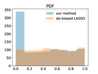
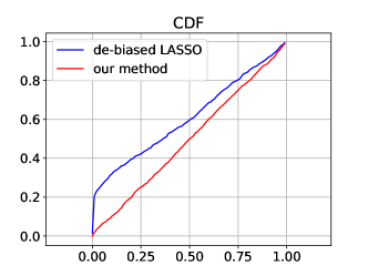
Figure 1: Distribution of two-sided Z-test p-values under the null hypothesis (high dimensional)

High dimensional linear regression.

Figure 1 shows p-value distribution under the null hypothesis for our method and the de-biased LASSO estimator with known covariance, using 600 i.i.d. samples generated from a model with $\Sigma=I$, $\sigma=0.7$, and we can see that it is close to a uniform distribution, similar results are observed for other high dimensional statistical inference procedures such as [CFJL18]. And visualization of confidence intervals computed by our algorithm is shown in Figure 3.

Time series analysis.

In our linear regression simulation, we generate i.i.d. random explanatory variables, and the observation noise is a 0-mean moving average (MA) process independent of the explanatory variables. Results on average 95% confidence interval coverage and length are given in Section H.1.3, and they validate our theory.

5.2 Real data

Neural network adversarial attack detection.

Here we use ideas from statistical inference to detect certain adversarial attacks on neural networks. A key observation is that neural networks are effective at representing low dimensional manifolds such as natural images [BJ16, CM16], and this causes the risk function’s Hessian to be degenerate [SEG⁺17]. From a statistical inference perspective, we interpret this as meaning that the confidence intervals in the null space of $H^{+}GH^{+}$ is infinity, where $H^{+}$ is the pseudo-inverse of the Hessian (see Section 2). When we make a prediction $\Psi(x;\widehat{\theta})$ using a fixed data point $x$ as input (i.e., conditioned on $x$), using the delta method [vdV98], the confidence interval of the prediction can be derived from the asymptotic normality of $\Psi(x;\widehat{\theta})$

$$\sqrt{n}\left(\Psi(x;\widehat{\theta})-\Psi(x;\theta^{\star})\right)\to\mathcal{N}\left(0,\nabla_{\theta}\Psi(x;\widehat{\theta})^{\top}\left[\widehat{H}^{-1}\widehat{G}\widehat{H}^{-1}\right]\nabla_{\theta}\Psi(x;\widehat{\theta})\right).$$

To detect adversarial attacks, we use the score

$$\tfrac{\left\|\left(I-P_{H^{+}GH^{+}}\right)\nabla_{\theta}\Psi(x;\widehat{\theta})\right\|_{2}}{\left\|\nabla_{\theta}\Psi(x;\widehat{\theta})\right\|_{2}},$$

to measure how much $\nabla_{\theta}\Psi(x;\widehat{\theta})$ lies in null space of $H^{+}GH^{+}$, where $P_{H^{+}GH^{+}}$ is the projection matrix onto the range of $H^{+}GH^{+}$. Conceptually, for the same image, the randomly perturbed image’s score should be larger than the original image’s score, and the adversarial image’s score should be larger than the randomly perturbed image’s score.

We train a binary classification neural network with 1 hidden layer and softplus activation function, to distinguish between “Shirt” and “T-shirt/top” in the Fashion MNIST data set [XRV17]. Figure 2 shows distributions of scores of original images, adversarial images generated using the fast gradient sign method [GSS14], and randomly perturbed images. Adversarial and random perturbations have the same $\ell_{\infty}$ norm. The adversarial perturbations and example images are shown in Section H.2.1. Although the scores’ values are small, they are still significantly larger than 64-bit floating point precision ($2^{-53}\approx 1.11\times 10^{-16}$). We observe that scores of randomly perturbed images is an order of magnitude larger than scores of original images, and scores of adversarial images is an order of magnitude larger than scores of randomly perturbed images.

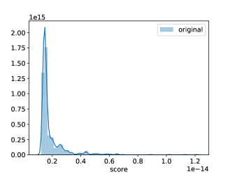
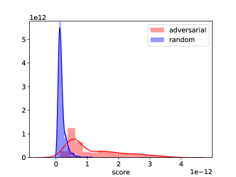
Figure 2: Distribution of scores for original, randomly perturbed, and adversarially perturbed images

High dimensional linear regression.

We apply our high dimensional inference procedure to the dataset in [RTW⁺06] to detect mutations related to HIV drug resistance, where we randomly sub-sample the dataset so that the number of features is larger than the number of samples. When we control the family-wise error rate (FWER) at $0.05$ using the Bonferroni correction [Bon36], our procedure is able to detect verified mutations in an expert dataset [JBVC⁺05] (Table 4), and the details are given in Section H.2.2. Another experiment with a genomic data set concerning riboflavin (vitamin B2) production rate [BKM14] is given in the appendix.

Time series analysis.

Using monthly equities returns data from [FP14], we use our approximate Newton statistical inference procedure to show that the correlation between US equities market returns and non-US global equities market returns is statistically significant, which validates the capital asset pricing model (CAPM) [Sha64, Lin65, FF04]. The details are given in Section H.2.3.

6 Related work

Unregularized M-estimation.

This work provides a general, flexible framework for simultaneous point estimation and statistical inference, and improves upon previous methods, based on averaged stochastic gradient descent [LLKC18, CLTZ16].

Compared to [CLTZ16] (and similar works [SZ18, FXY17] using SGD with decreasing step size), our method does not need to increase the lengths of “segments” (inner loops) to reduce correlations between different “replicates”. Even in that case, if we use $T$ replicates and increasing “segment” length (number of inner loops is $t^{\frac{d_{o}}{1-d_{o}}}\cdot L$) with a total of $O(T^{\frac{1}{1-d_{o}}}\cdot L)$ stochastic gradient steps, [CLTZ16] guarantees $O(L^{-\frac{1-d_{o}}{2}}+T^{-\frac{1}{2}}+T^{\max\{\frac{1}{2}-\frac{d_{o}}{4(1-d_{o})},0\}-\frac{1}{2}}\cdot L^{-\frac{d_{o}}{4}}+T^{\max\{\frac{1-2d_{o}}{2(1-d_{o})},0\}-\frac{1}{2}}\cdot L^{\frac{1-2d_{o}}{2}})$ , whereas our method guarantees $O(T^{-\frac{d_{o}}{2}})$. Further, [CLTZ16] is inconsistent, whereas our scheme guarantees consistency of computing the statistical error covariance.

[LLKC18] uses fixed step size SGD for statistical inference, and discards iterates between different “segments” to reduce correlation, whereas we do not discard any iterates in our computations. Although [LLKC18] states empirically constant step SGD performs well in statistical inference, it has been empirically shown [DDB17] that averaging consecutive iterates in constant step SGD does not guarantee convergence to the optimal – the average will be “wobbling” around the optimal, whereas decreasing step size stochastic approximation methods ([PJ92, Rup88] and our work) will converge to the optimal, and averaging consecutive iterates guarantees “fast” rates.

Finally, from an optimization perspective, our method is similar to stochastic Newton methods (e.g. [ABH17]); however, our method only uses first-order information to approximate a Hessian vector product ($\nabla^{2}f(\theta)v\approx\tfrac{\nabla f(\theta+\delta v)-\nabla f(\theta)}{\delta}$). Algorithm 1’s outer loops are similar to stochastic natural gradient descent [Ama98]. Also, we demonstrate an intuitive view of SVRG [JZ13] as a special case of approximate stochastic Newton steps using first order information (Appendix E).

High dimensional linear regression.

[CLTZ16]’s high dimensional inference algorithm is based on [ANW12], and only guarantees that optimization error is at the same scale as the statistical error. However, proper de-biasing of the LASSO estimator requires the optimization error to be much less than the statistical error, otherwise the optimization error introduces additional bias that de-biasing cannot handle. Our optimization objective is strongly convex with high probability: this permits the use of linearly convergent proximal algorithms [XZ14, LSS14] towards the optimum, which guarantees the optimization error to be much smaller than the statistical error.

Our method of de-biasing the LASSO in Section 3 is similar to [ZZ14, vdGBRD14, JM14, JM15]. Our method uses a new $\ell_{1}$ regularized objective (13) for high dimensional linear regression, and we have different de-biasing terms, because we also need to de-bias the covariance estimation. In Algorithm 2, our covariance estimate is similar to the classic sandwich estimator [Hub67, Whi80]. Previous methods require $O(p^{2})$ space which unsuitable for large scale problems, whereas our method only requires $O(p)$ space.

Similar to our $\ell_{1}$-norm regularized objective, [YLR14, JD11] shows similar point estimate statistical guarantees for related estimators; however there are no confidence interval results. Further, although [YLR14] is an elementary estimator in closed form, it still requires computing the inverse of the thresholded covariance, which is challenging in high dimensions, and may not computationally outperform optimization approaches.

Finally, for feature selection, we do not assume that absolute values of the true parameter’s non-zero entries are lower bounded (“beta-min” condition). [FGLS18, Loh17, LW17, BvdG11, Wai09].

Time series analysis.

Our approach of sampling contiguous blocks of indices to compute stochastic gradients for statistical inference in time series analysis is similar to resampling procedures in moving block or circular bootstrap [Car86, Kun89, Büh02, DH97, ET94, Lah13, PR92, PR94, KL12], and conformal prediction [BHV14, SV08, VGS05]. Also, our procedure is similar to Driscoll-Kraay standard errors [DK98, KD99, Hoe07], but does not waste computational resources to explicitly store entire matrices, and is suited for large scale time series analysis.

Appendix A High dimensional linear regression statistical inference using stochastic gradients (Section 3)

A.1 Statistical inference using approximate proximal Newton steps with stochastic gradients

Here, we present a statistical inference procedure for high dimensional linear regression via approximate proximal Newton steps using stochastic gradients. It uses the plug-in estimator:

$$\widehat{S}^{-1}\left(\tfrac{1}{n}\sum_{i=1}^{n}(x_{i}^{\top}\widehat{\theta}-y_{i})^{2}x_{i}x_{i}^{\top}\right)\widehat{S}^{-1},$$

which is related to the empirical sandwich estimator [Hub67, Whi80]. Lemma 1 shows this is a good estimate of the covariance when $n\gg\tfrac{1}{{D_{\Sigma}}^{4}}\max\{1,\sigma^{2}\}s^{2}(\sigma+\|\theta^{\star}\|_{1})^{2}$.

Algorithm 2 performs statistical inference in high dimensional linear regression (13), by computing the statistical error covariance in Theorem 3, based on the plug-in estimate in Lemma 1. We denote the soft thresholding of $A$ by $\omega$ as an element-wise procedure $\left(\operatorname{\mathbf{S}}_{\omega}(A)\right)_{e}=\operatorname{sign}(A_{e})(|A_{e}|-\omega)_{+}$. For a vector $v$, we write $v$’s $i$^th coordinate as $v(i)$. The optimization objective (13) is denoted as:

$$\tfrac{1}{2}\theta^{\top}\left(\widehat{S}-\tfrac{1}{n}{\mathop{\textstyle\sum}}_{i=1}^{n}x_{i}x_{i}^{\top}\right)\theta+\tfrac{1}{n}{\mathop{\textstyle\sum}}_{i=1}^{n}f_{i},$$

where $f_{i}=\tfrac{1}{2}\left(x_{i}^{\top}-y_{i}\right)^{2}.$ Further,

$$\bm{g}_{\widehat{S}}(v)=\nabla_{v}\left[\tfrac{1}{2}v^{\top}\widehat{S}v\right]=\widehat{S}v=\sum_{j=1}^{p}v(j)\cdot\operatorname{\mathbf{S}}_{\omega}\left(\tfrac{1}{n}\sum_{i=1}^{n}\left[\nabla f_{i}(\theta+{\bm{e}}_{j})-\nabla f_{i}(\theta)\right]\right),$$

where ${\bm{e}}_{i}\in\mathbb{R}^{p}$ is the basis vector where the $i$^th coordinate is $1$ and others are $0$, and $\widehat{S}v$ is computed in a column-wise manner.

For point estimate optimization, the proximal Newton step [LSS14] at $\theta$ solves the optimization problem

$$\min_{\Delta}\tfrac{1}{2\rho}\Delta^{\top}\widehat{S}\Delta+\left\langle(\widehat{S}-\tfrac{1}{n}{\mathop{\textstyle\sum}}_{i=1}^{n}x_{i}x_{i}^{\top})\theta+\tfrac{1}{n}\sum_{i=1}^{n}\nabla f_{i}(\theta),\Delta\right\rangle+\lambda\|\theta+\Delta\|_{1},$$

to determine a descent direction. For statistical inference, we solve a Newton step:

$$\min_{\Delta}\tfrac{1}{2\rho}\Delta^{\top}\widehat{S}\Delta+\left\langle\tfrac{1}{S_{o}}\sum_{k\in I_{o}}\nabla f_{k}(\theta_{t}),\Delta\right\rangle$$

to compute $-\widehat{S}^{-1}\frac{1}{S_{o}}\sum_{i\in I_{o}}\nabla f_{i}(\theta)$, whose covariance is the statistical error covariance.

To control variance, we solve Newton steps using SVRG and proximal SVRG [XZ14], because in the high dimensional setting, the variance using SGD [MB11] and proximal SGD [AFM17] for solving Newton steps is too large. However because $p\gg n$, instead of sampling by sample, we sample by feature. We start from $\theta_{0}$ sufficiently close to $\widehat{\theta}$ (see Theorem 4 for details), which can be effectively achieved using proximal SVRG (Section A.3). Line 7 corresponds to SVRG’s outer loop part that computes the full gradient, and line 12 corresponds to SVRG’s inner loop update. Line 8 corresponds to proximal SVRG’s outer loop part that computes the full gradient, and line 13 corresponds to proximal SVRG’s inner loop update.

The covariance estimate bound, asymptotic normality result, and choice of hyper-parameters are described in Section A.4. When $L_{o}^{t}=\Theta(\log(p)\cdot\log(t))$, we can estimate the covariance with element-wise error less than $O\left(\frac{\max\{1,\sigma\}{\operatorname{polylog}}(n,p)}{\sqrt{T}}\right)$ with high probability, using $O\left(T\cdot n\cdot p^{2}\cdot\log(p)\cdot\log(T)\right)$ numerical operations. Calculation of the de-biased estimator $\widehat{\theta}^{\mathrm{d}}$ (16) via SVRG is described in Section A.2.

1:  Parameters: $S_{o},S_{i}\in\mathbb{Z}_{+}$; $\eta,\tau\in\mathbb{R}_{+}$;  Initial state: $\theta_{0}\in\mathbb{R}^{p}$  

2:  for $t=0$ to $T-1$ do

3:     $I_{o}\leftarrow$ uniformly sample $S_{o}$ indices with replacement from $[n]$

4:     $g_{t}^{0}\leftarrow-\frac{1}{S_{o}}\sum_{k\in I_{o}}\nabla f_{k}(\theta_{t})$

5:     $d_{t}^{0}\leftarrow-\left(\bm{g}_{\widehat{S}}(\theta_{t})-\frac{1}{n}\sum_{i=1}^{n}\left[\nabla f_{i}(\theta_{t}+\theta_{t})-\nabla f_{i}(\theta_{t})\right]+\tfrac{1}{n}{\mathop{\textstyle\sum}}_{i=1}^{n}\nabla f_{i}(\theta_{t})\right)$

6:     for $j=1$ to $L_{o}^{t}-$ do  // solving Newton steps using SVRG

7:        $u_{t}^{j}\leftarrow\bm{g}_{\widehat{S}}(g_{t}^{j-1})-g_{t}^{0}$

8:        $v_{t}^{j}\leftarrow\bm{g}_{\widehat{S}}(d_{t}^{j-1})-d_{t}^{0}$

9:        $g_{t}^{j}\leftarrow g_{t}^{j-1}$, $d_{t}^{j}\leftarrow d_{t}^{j-1}$

10:        for $l=1$ to $L_{i}$ do

11:           $I_{i}\leftarrow$ uniformly sample $S_{i}$ indices without replacement from $[p]$

12:           $g_{t}^{j}\leftarrow g_{t}^{j}-\tau\left[u_{t}^{j}+\frac{p}{S_{i}}\sum_{k\in S_{i}}\left[g_{t}^{j}(k)-g_{t}^{j-1}(k)\right]\cdot\operatorname{\mathbf{S}}_{\omega}\left(\nabla f_{k}(\theta_{t}+{\bm{e}}_{k})-\nabla f_{k}(\theta_{t})\right)\right]$

13:           $d_{t}^{j}\leftarrow\operatorname{\mathbf{S}}_{\eta\lambda}\left(d_{t}^{j}-\eta\left[v_{t}^{j}+\frac{p}{S_{i}}\sum_{k\in S_{i}}\left[d_{t}^{j}(k)-d_{t}^{j-1}(k)\right]\cdot\operatorname{\mathbf{S}}_{\omega}\left(\nabla f_{k}(\theta_{t}+{\bm{e}}_{k})-\nabla f_{k}(\theta_{t})\right)\right]\right)$

14:        end for

15:     end for

16:     Use $\sqrt{S_{o}}\cdot\frac{\bar{g}_{t}}{\rho_{t}}$ for statistical inference, where $\bar{g}_{t}=\frac{1}{L_{o}^{t}+1}\sum_{j=0}^{L_{o}^{t}}g_{t}^{j}$

17:     $\theta_{t+1}=\theta_{t}+\bar{d}_{t}$, where $\bar{d}_{t}=\frac{1}{L_{o}+1}\sum_{j=0}^{L_{o}^{t}}d_{t}^{j}$  // point estimation (optimization)

18:  end for

Algorithm 2 High dimensional linear regression statistical inference

A.2 Computing the de-biased estimator (16) via SVRG

To control variance, we solve each proximal Newton step using SVRG, in stead of SGD as in Algorithm 1. Because However because the number of features is much larger than the number of samples, instead of sampling by sample, we sample by feature.

The de-biased estimator is

$$\widehat{\theta}^{\mathrm{d}}= \widehat{\theta}+\widehat{S}^{-1}\left[\frac{1}{n}\sum_{i=1}^{n}y_{i}x_{i}-\left(\frac{1}{n}\sum_{i=1}^{n}x_{i}x_{i}^{\top}\right)\widehat{\theta}\right]$$

$$= \widehat{\theta}+\widehat{S}^{-1}\left(-\frac{1}{n}\sum_{i=1}^{n}\nabla f_{i}(\widehat{\theta})\right).$$

And we compute $\widehat{S}^{-1}\frac{1}{n}\sum_{i=1}^{n}\nabla f_{i}(\widehat{\theta})$ using SVRG [JZ13] by solving the following optimization problem using SVRG and sampling by feature

$$\min_{u}\frac{1}{2}u^{\top}\widehat{S}u+\left\langle\frac{1}{n}\sum_{i=1}^{n}\nabla f_{i}(\widehat{\theta}),u\right\rangle.$$

1:  for $i=0$ to $L_{o}-1$ do

2:     $d_{i}^{0}\leftarrow-\eta[\bm{g}_{\widehat{S}}(u_{i})+\frac{1}{n}\sum_{k=1}^{n}\nabla f_{k}(\widehat{\theta})]$

3:     for $j=0$ to $L_{i}-1$ do

4:        $I\leftarrow$ sample $S$ indices uniformly from $[p]$ without replacement

5:        $d_{i}^{j+1}\leftarrow d_{i}^{j}+d_{t}^{0}-\eta\left(\frac{1}{S}\sum_{k\in I}d_{i}^{j}(k)\cdot\operatorname{\mathbf{S}}_{\omega}(\nabla f_{k}(\widehat{\theta}+{\bm{e}}_{k})-f_{k}(\widehat{\theta}))\right)$

6:     end for

7:     $u_{i+1}\leftarrow u_{i}+\bar{d}_{i}$, where $\bar{d}_{i}=\frac{1}{L_{i}+1}\sum_{j=0}^{L_{i}}d_{i}^{j}$

8:  end for

Algorithm 3 Computing the de-biased estimator (16) via SVRG

Similar to Algorithm 2, we choose $\eta=\Theta\left(\frac{1}{p}\right)$ and $L_{i}=\Theta(p)$.

A.3 Solving the high dimensional linear regression optimization objective (13) using proximal SVRG

We solve our high dimensional linear regression optimization problem using proximal SVRG [XZ14]

$$\widehat{\theta}=\arg\min_{\theta}\frac{1}{2}\theta^{\top}\left(\widehat{S}-\frac{1}{n}\sum_{i=1}^{n}x_{i}x_{i}^{\top}\right)\theta+\frac{1}{n}\sum_{i=1}^{n}\frac{1}{2}\left(x_{i}^{\top}\theta-y_{i}\right)^{2}+\lambda\|{\theta}\|_{1}.$$ (20)

1:  for $i=0$ to $L_{o}-1$ do

2:     $u_{i}^{0}\leftarrow\theta_{i}$

3:     $d_{t}\leftarrow\bm{g}_{\widehat{S}}(\theta_{i})-\frac{1}{n}\sum_{k=1}^{n}[\nabla f_{k}(\theta_{i}+\theta_{i})-\nabla f_{k}(\theta_{i})]+\frac{1}{n}\sum_{k=1}^{n}\nabla f_{k}(\theta_{i})$

4:     for $j=0$ to $L_{i}-1$ do

5:        $u_{i}^{j+1}$ $\leftarrow$ $\operatorname{\mathbf{S}}_{\eta\lambda}(u_{i}^{j}-\eta[d_{t}+\frac{1}{S}\sum_{k\in I}\left(u_{i}^{j}(k)-\theta_{i}(k)\right)\cdot\operatorname{\mathbf{S}}_{\omega}\left(\nabla f_{k}(\theta_{t}+{\bm{e}}_{k})-\nabla f_{k}(\theta_{t})\right)])$

6:     end for

7:     $\theta_{t+1}\leftarrow\frac{1}{L_{i}+1}\sum_{j=0}^{L_{i}}u_{i}^{j}$

8:  end for

Algorithm 4 Solving the high dimensional linear regression optimization objective (13) using proximal SVRG

Similar to Algorithm 2, we choose $\eta=\Theta\left(\frac{1}{p}\right)$ and $L_{i}=\Theta(p)$.

A.4 Non-asymptotic covariance estimate bound and asymptotic normality in Algorithm 2

We have a non-asymptotic covariance estimate bound and an asymptotic normality result.

Theorem 4.

Under our assumptions, when $n\gg\max\{b^{2},\frac{1}{{D_{\Sigma}}^{2}}\}\log p$, $S_{o}=O(1)$, $S_{i}=O(1)$, and conditioned on $\{x_{i}\}_{i=1}^{n}$ and following events which simultaneously with probability at least $1-p^{-\Theta(1)}-n^{-\Theta(1)}$

• [A]: $\max_{1\leq i\leq n}|\epsilon_{i}|\lesssim\sigma\sqrt{\log n}$,

• [B]: $\max_{1\leq i\leq n}\|x_{i}\|_{\infty}\lesssim\sqrt{\log p+\log n}$,

• [C]: $\|{\widehat{S}}^{-1}\|_{\infty}\lesssim\frac{1}{D_{\Sigma}}$,

we choose $L_{i}=\Theta(p)$, $\tau=\Theta(\frac{1}{p})$, $\eta=\Theta(\frac{1}{p})$ in Algorithm 2.

Here, we denote the objective function as

$$P(\theta)=\frac{1}{2}\theta^{\top}\left(\widehat{S}-\frac{1}{n}\sum_{i=1}^{n}x_{i}x_{i}^{\top}\right)\theta+\frac{1}{n}\sum_{i=1}^{n}\frac{1}{2}\left(x_{i}^{\top}\theta-y_{i}\right)^{2}+\lambda\|{\theta}\|_{1}.$$

Then, we have a non-asymptotic covariance estimate bound

$$\left\|\tfrac{S_{o}}{T}{\mathop{\textstyle\sum}}_{t=1}^{T}\bar{g}_{t}\bar{g}_{t}^{\top}-{\widehat{S}}^{-1}\left(\tfrac{1}{n}{\mathop{\textstyle\sum}}_{i=1}^{n}(x_{i}^{\top}\widehat{\theta}-y_{i})^{2}x_{i}x_{i}^{\top}\right){\widehat{S}}^{-1}\right\|_{\max}$$

$$\lesssim \sqrt{\left((\log p+\log n)\|\widehat{\theta}-\theta^{\star}\|_{1}+\sigma\sqrt{(\log p+\log n)\log n}\right)\tfrac{\log p}{T}}$$

$$+\tfrac{1}{u}\left[\tfrac{1}{\sqrt{T}}{\mathop{\textstyle\sum}}_{t=1}^{T}0.95^{L_{o}^{t}}(1+\sqrt{P(\theta_{0})-P(\widehat{\theta})}0.95^{\sum_{i=0}^{t-1}L_{o}^{t}})+\sqrt{p}(\log p+\log n)\sqrt{P(\theta_{0})-P(\widehat{\theta})}0.95^{\sum_{i=0}^{t-1}L_{o}^{t}}\right],$$

where $\|A\|_{\max}=\max\{1\leq j,k\leq p\}|A_{jk}|$ is the matrix max norm, with probability at least $1-p^{-\Theta(-1)}-u$.

And we have asymptotic normality

$$\tfrac{1}{\sqrt{t}}\left({\mathop{\textstyle\sum}}_{t=1}^{T}\sqrt{S_{o}}\bar{g_{t}}+\tfrac{1}{n}{\mathop{\textstyle\sum}}_{i=1}^{n}x_{i}(x_{i}^{\top}\widehat{\theta}-y_{i})\right)=W+R,$$

where $W$ weakly converges to $\scriptstyle\mathcal{N}\left(0,\widehat{S}^{-1}\left[\frac{1}{n}\sum_{i=1}^{n}(x_{i}^{\top}\widehat{\theta}-y_{i})^{2}x_{i}x_{i}^{\top}-\left(\frac{1}{n}\sum_{i=1}^{n}x_{i}(x_{i}^{\top}\widehat{\theta}-y_{i})\right)\left(\frac{1}{n}\sum_{i=1}^{n}x_{i}(x_{i}^{\top}\widehat{\theta}-y_{i})\right)^{\top}\right]\widehat{S}^{-1}\right)$, and ${\operatorname{\mathbb{E}}}[\|R\|_{\infty}\mid\{x_{i}\}_{i=1}^{n},\ref{mytag:thm:alg:stat-inf:high-dim:linear:proximal:svrg:event-A},\ref{mytag:thm:alg:stat-inf:high-dim:linear:proximal:svrg:event-B},\ref{mytag:thm:alg:stat-inf:high-dim:linear:proximal:svrg:event-C}]\lesssim\frac{1}{\sqrt{T}}\sum_{t=1}^{T}0.95^{L_{o}^{t}}(1+\sqrt{P(\theta_{0})-P(\widehat{\theta})}0.95^{\sum_{i=0}^{t-1}L_{o}^{t}})+\sqrt{p}(\log p+\log n)\sqrt{P(\theta_{0})-P(\widehat{\theta})}0.95^{\sum_{i=0}^{t-1}L_{o}^{t}}$.

Note that when we choose $L_{o}^{t}=\Theta(\log(p)\cdot\log(t))$, and start from $\theta_{0}$ satisfying $P(\theta_{0})-P(\widehat{\theta})\lesssim\frac{1}{p(\log p+\log n)^{2}}$ which can be effectively achieved using proximal SVRG (Section A.3), we can estimate the statistical error covariance with element-wise error less than $O\left(\frac{\max\{1,\sigma\}{\operatorname{polylog}}(n,p)}{\sqrt{T}}\right)$ with high probability, using $O\left(T\cdot n\cdot p^{2}\cdot\log(p)\cdot\log(T)\right)$ numerical operations.

A.5 Plug-in statistical error covariance estimate

Algorithm 2 is similar to using plug-in estimator $\frac{1}{n}\sum_{i=1}^{n}(x_{i}^{\top}\widehat{\theta}-y_{i})^{2}x_{i}x_{i}^{\top}$ for $\sigma^{2}\left(\frac{1}{n}\sum_{i=1}^{n}x_{i}x_{i}^{\top}\right)$ in Theorem 3, similar to the sandwich estimator [Hub67, Whi80]. Lemma 1 gives a bound on using this plug-in estimator in the statistical error covariance (Theorem 3) for coordinate-wise confidence intervals.

Lemma 1.

Under our assumptions, when $n\gg\max\{b^{2},\tfrac{1}{{D_{\Sigma}}^{2}}\}\log p$, we have

$$\left\|\widehat{S}^{-1}\left(\tfrac{1}{n}{\mathop{\textstyle\sum}}_{i=1}^{n}(x_{i}^{\top}\widehat{\theta}-y_{i})^{2}x_{i}x_{i}^{\top}\right)\widehat{S}^{-1}-\sigma^{2}\widehat{S}^{-1}\left(\tfrac{1}{n}{\mathop{\textstyle\sum}}_{i=1}^{n}x_{i}x_{i}^{\top}\right)\widehat{S}^{-1}\right\|_{\max}$$

$$\lesssim \tfrac{1}{{D_{\Sigma}}^{2}}\left(\sigma\sqrt{\log n}+s\left(\sigma+\|\theta^{\star}\|_{1}\right)\sqrt{\log p+\log n}\sqrt{\tfrac{\log p}{n}}\right)s\left(\sigma+\|\theta^{\star}\|_{1}\right)(\log p+\log n)^{\frac{3}{2}}\sqrt{\tfrac{\log p}{n}},$$

where $\|A\|_{\max}=\max_{1\leq j,k\leq p}|A_{jk}|$ is the matrix max norm, with probability at least $1-p^{-\Theta(1)}-n^{-\Theta(1)}$.

Appendix B Time series statistical inference with approximate Newton steps using only stochastic gradients (Section 4)

Here, we give the complete approximate Newton-based time series statistical inference algorithm using only stochastic gradients.

1:  Parameters: $\mathbf{l},S_{i}\in\mathbb{Z}_{+}$; $\rho_{0},\tau_{0}\in\mathbb{R}_{+}$; $d_{o},d_{i}\in\left(\tfrac{1}{2},1\right)$  Initial state: $\theta_{0}\in\mathbb{R}^{p}$  

2:  for $t=0\text{ to }T-1$ do  // approximate stochastic Newton descent

3:     $\rho_{t}\leftarrow\rho_{0}(t+1)^{-d_{o}}$

4:     Uniformly select some $i_{o}\in[n]$, then set $I_{o}$ to the random contiguous block $\{i_{o},i_{o}+1,\dots,i_{o}+\mathbf{l}-1\}\mod n$, which circularly wraps around

5:     $g^{0}_{t}\leftarrow-\rho_{t}\left(\frac{1}{\mathbf{l}}\sum_{i\in I_{o}}\nabla f_{i}(\theta_{t})\right)$

6:     for $j=0\text{ to }L-1$ do  // solving (1) approximately using SGD

7:        $\tau_{j}\leftarrow\tau_{0}(j+1)^{-d_{i}}$ and $\delta_{t}^{j}\leftarrow O(\rho_{t}^{4}\tau_{j}^{4})$

8:        $I_{i}\leftarrow$ uniformly sample $S_{i}$ indices without replacement from $[n]$

9:        $g^{j+1}_{t}\leftarrow g_{t}^{j}-\tau_{j}\left(\frac{1}{S_{i}}\sum_{k\in I_{i}}\tfrac{\nabla f_{k}(\theta_{t}+{\delta_{t}^{j}}g_{t}^{j})-\nabla f_{k}(\theta_{t})}{\delta_{t}^{j}}\right)+\tau_{j}g_{t}^{0}$

10:     end for

11:     Use $\sqrt{\mathbf{l}}\cdot\frac{\bar{g}_{t}}{\rho_{t}}$ for statistical inference, where $\bar{g}_{t}=\frac{1}{L+1}\sum_{j=0}^{L}g^{j}_{t}$

12:     $\theta_{t+1}\leftarrow\theta_{t}+g_{t}^{L}$

13:  end for

Algorithm 5 Unregularized M-estimation statistical inference

Corollary 2 gives guarantees for Algorithm 5, and is similar to the i.i.d. case (Theorem 1).

Corollary 2.

Under the same assumptions as Theorem 1, in Algorithm 5, for the outer iterate $\theta_{t}$ we have

$${\operatorname{\mathbb{E}}}\left[\|\theta_{t}-\widehat{\theta}\|_{2}^{2}\right] \lesssim t^{-d_{o}},$$ (21)

$${\operatorname{\mathbb{E}}}\left[\|\theta_{t}-\widehat{\theta}\|_{2}^{4}\right] \lesssim t^{-2d_{o}}.$$ (22)

In each outer loop, after $L$ steps of the inner loop, we have:

$${\operatorname{\mathbb{E}}}\left[\left\|\tfrac{\bar{g}_{t}}{\rho_{t}}-[\nabla^{2}f(\theta_{t})]^{-1}g_{t}^{0}\right\|_{2}^{2}\mid\theta_{t}\right]\lesssim\tfrac{1}{L}\left\|g_{t}^{0}\right\|_{2}^{2},$$ (23)

and at each step of the inner loop, we have:

$${\operatorname{\mathbb{E}}}\left[\left\|g_{t}^{j+1}-[\nabla^{2}f(\theta_{t})]^{-1}g_{t}^{0}\right\|_{2}^{4}\mid\theta_{t}\right]\lesssim(j+1)^{-2d_{i}}\left\|g_{t}^{0}\right\|_{2}^{4}.$$ (24)

After $T$ steps of the outer loop, we have a non-asymptotic bound on the “covariance”:

$${\operatorname{\mathbb{E}}}\left[\left\|H^{-1}GH^{-1}-\tfrac{S_{o}}{T}\sum_{t=1}^{T}\tfrac{\bar{g}_{t}\bar{g}_{t}^{\top}}{\rho_{t}^{2}}\right\|_{2}\right]\lesssim T^{-\frac{d_{o}}{2}}+L^{-\frac{1}{2}},$$ (25)

where $H=\nabla^{2}f(\widehat{\theta})$, and

$$G=\tfrac{1}{n}\sum\limits_{i=1}^{n}\nabla f_{i}(\widehat{\theta})\,f_{i}(\widehat{\theta})^{\top}+\sum\limits_{j=1}^{\mathbf{l}}w(j,\mathbf{l})\sum\limits_{i=j+1}^{n}\left(\nabla f_{i}(\widehat{\theta})\,\nabla f_{i-j}(\widehat{\theta})^{\top}+\nabla f_{i-j}(\widehat{\theta})\,\nabla f_{i}(\widehat{\theta})^{\top}\right),$$ (26)

with $w(j,\mathbf{l})=1-\tfrac{j}{\mathbf{l}}$.

Also, in Algorithm 5’s outer loop, the average of consecutive iterates satisfies

$${\operatorname{\mathbb{E}}}\left[\left\|\tfrac{\sum_{t=1}^{T}\theta_{t}}{T}-\widehat{\theta}\right\|_{2}^{2}\right] \lesssim\tfrac{1}{T},$$ (27)

$$\tfrac{1}{\sqrt{T}}\left(\tfrac{\sum_{t=1}^{T}\theta_{t}}{T}-\widehat{\theta}\right) =W+\Delta,$$ (28)

where $W$ weakly converges to $\mathcal{N}(0,\frac{1}{S_{o}}H^{-1}GH^{-1})$, and $\Delta=o_{P}(1)$ when $T\to\infty$ and $L\to\infty$ (${\operatorname{\mathbb{E}}}[\|\Delta\|_{2}^{2}]$ $\lesssim$ $T^{1-2d_{o}}+T^{d_{o}-1}+\frac{1}{L}$).

Our approximate Newton time series statistical inference procedure estimates $H^{-1}GH^{-1}$, where $G$ is the Newey-West covariance estimator (19) with weight

$$w(j,\mathbf{l})=1-\tfrac{j}{\mathbf{l}},$$ (29)

which is because when we estimate the variance in Algorithm 5, for $j>0$, terms $\nabla f_{i}\,\nabla f_{i+j}^{\top}$ and $\nabla f_{i+j}\,\nabla f_{i}^{\top}$ appear $\mathbf{l}-j$ times, and the term $\nabla f_{i}\,\nabla f_{i}^{\top}$ appears $\mathbf{l}$ times. Note that the connection between sampling scheme and Newey-West estimator was also observed in [Kun89]. Thus, our stochastic approximate Newton statistical inference procedure for time series analysis has similar statistical properties compared circular bootstrap [PR92, PR94].

Because expectation of the stochastic gradient in line 5 of Algorithm 5 is the full gradient $\frac{1}{n}\sum_{i=1}^{n}f_{i}(\widehat{\theta})$, we have the same optimization guarantees as the i.i.d. case (Corollary 1).

Appendix C Statistical inference via approximate stochastic Newton steps using first order information with increasing inner loop counts

Here, we present corollaries when the number of inner loops increases in the outer loops (i.e., $(L)_{t}$ is an increasing series). This guarantees convergence of the covariance estimate to $H^{-1}GH^{-1}$, although it is less efficient than using a constant number of inner loops.

C.1 Unregularized M-estimation

Similar to Theorem 1’s proof, we have the following result when the number of inner loop increases in the outer loops.

Corollary 3.

In Algorithm 1, if the number of inner loop in each outer loop $(L)_{t}$ increases in the outer loops, then we have

$${\operatorname{\mathbb{E}}}\left[\left\|H^{-1}GH^{-1}-\frac{S_{o}}{T}\sum_{t=1}^{T}\frac{\bar{g}_{t}\bar{g}_{t}^{\top}}{\rho_{t}^{2}}\right\|_{2}\right]\lesssim T^{-\frac{d_{o}}{2}}+\sqrt{\frac{1}{T}\sum_{i=1}^{T}\frac{1}{(L)_{t}}}.$$

For example, when we choose choose $(L)_{t}=L(t+1)^{d_{L}}$ for some $d_{L}>0$, then $\sqrt{\frac{1}{T}\sum_{i=1}^{T}\frac{1}{(L)_{t}}}=O(\frac{1}{\sqrt{L}}T^{-\frac{d_{L}}{2}})$.

Appendix D SVRG based statistical inference algorithm in unregularized M-estimation

Here we present a SVRG based statistical inference algorithm in unregularized M-estimation, which has asymptotic normality and improved bounds for the “covariance”. Although Algorithm 6 has stronger guarantees than Algorithm 1, Algorithm 6 requires a full gradient evaluation in each outer loop.

1:  for $t\leftarrow 0;t<T;++t$ do

2:     $d^{0}_{t}\leftarrow-\eta\nabla f(\theta_{t})=-\eta\left(\frac{1}{n}\sum_{i=1}^{n}\nabla f_{i}(\theta)\right)$  // point estimation via SVRG

3:     $I_{o}\leftarrow$ uniformly sample $S_{o}$ indices with replacement from $[n]$

4:     $g^{0}_{t}\leftarrow-\rho_{t}\left(\frac{1}{S_{o}}\sum_{i\in I_{o}}\nabla f_{i}(\theta_{t})\right)$  // statistical inference

5:     for $j\leftarrow 0;j<L;++j$ do  // solving (1) approximately using SGD

6:        $I_{i}\leftarrow$ uniformly sample $S_{i}$ indices without replacement from $[n]$

7:        $d^{j+1}_{t}\leftarrow d_{t}^{j}-\eta\left(\frac{1}{S_{i}}\sum_{k\in I_{i}}(\nabla f_{k}(\theta_{t}+d_{t}^{j})-\nabla f_{k}(\theta_{t})\right)+d_{t}^{0}$  // point estimation via SVRG

8:        $g^{j+1}_{t}\leftarrow g_{t}^{j}-\tau_{j}\left(\frac{1}{S_{i}}\sum_{k\in I_{i}}\frac{1}{{\delta_{t}^{j}}}[\nabla f_{k}(\theta_{t}+{\delta_{t}^{j}}g_{t}^{j})-\nabla f_{k}(\theta_{t})]\right)+\tau_{j}g_{t}^{0}$  // statistical inference

9:     end for

10:     Use $\sqrt{S_{o}}\cdot\frac{\bar{g}_{t}}{\rho_{t}}$ for statistical inference  // $\bar{g}_{t}=\frac{1}{L+1}\sum_{j=0}^{L}g^{j}_{t}$

11:     $\theta_{t+1}\leftarrow\theta_{t}+\bar{d}_{t}$  // $\bar{d}_{t}=\frac{1}{L+1}\sum_{j=0}^{L}d^{j}_{t}$

12:  end for

Algorithm 6 SVRG based statistical inference algorithm in unregularized M-estimation

Corollary 4.

In Algorithm 6, when $L\geq 20\frac{\max_{1\leq i\leq n}\beta_{i}}{\alpha}$ and $\eta=\frac{1}{10\max_{1\leq i\leq n}\beta_{i}}$, after $T$ steps of the outer loop, we have a non-asymptotic bound on the “covariance”

$${\operatorname{\mathbb{E}}}\left[\left\|H^{-1}GH^{-1}-\frac{S_{o}}{T}\sum_{t=1}^{T}\frac{\bar{g}_{t}\bar{g}_{t}^{\top}}{\rho_{t}^{2}}\right\|_{2}\right]\lesssim L^{-\frac{1}{2}},$$ (30)

and asymptotic normality

$$\frac{1}{\sqrt{T}}(\sum_{t=1}^{T}\frac{\bar{g}_{t}}{\rho_{t}})=W+\Delta,$$

where $W$ weakly converges to $\mathcal{N}(0,\frac{1}{S_{o}}H^{-1}GH^{-1})$ and $\Delta=o_{P}(1)$ when $T\to\infty$ and $L\to\infty$ (${\operatorname{\mathbb{E}}}[\|\Delta\|_{2}]\lesssim\frac{1}{\sqrt{T}}+\frac{1}{L}$).

When the number of inner loops increases in the outer loops (i.e., $(L)_{t}$ is an increasing series), we have a result similar to Corollary 3.

A better understanding of concentration, and Edgeworth expansion of the average consecutive iterates averaged (beyond [Dip08a, Dip08b]) in stochastic approximation, would give stronger guarantees for our algorithms, and better compare and understand different algorithms.

D.1 Lack of asymptotic normality in Algorithm 1 for mean estimation

In mean estimation, we solve the following optimization problem

$$\widehat{\theta}=\arg\min_{\theta}\frac{1}{n}\sum_{i=1}^{n}\frac{1}{2}\|\theta-X^{(i)}\|_{2}^{2},$$

where we assume that $\{X^{(i)}\}_{i=1}^{n}$ are constants.

For ease of explanation we use $S_{o}=1$, $\rho_{t}=\rho$, and $\theta_{0}=0$,and we have

$$\frac{\bar{g_{t}}}{\rho_{t}}=-\theta_{t}+X_{t},$$

where $X_{t}$ is uniformly sampled from $\{X^{(i)}\}_{i=1}^{n}$.

And for $t\geq 1$ we have

$$\theta_{t}=\sum_{i=0}^{t-1}\rho(1-\rho)^{t-1-i}X_{i}.$$

Then, we have

$$\frac{1}{\sqrt{T}}(\sum_{i=1}^{T}\frac{\bar{g_{t}}}{\rho_{t}})$$

$$= \frac{1}{\sqrt{T}}(\sum_{t=1}^{T}X_{t}-\sum_{t=1}^{T}\sum_{i=0}^{t-1}\rho(1-\rho)^{t-1-i}X_{i})$$

$$= \frac{1}{\sqrt{T}}(\sum_{t=1}^{T}X_{t}-\sum_{i=0}^{T-1}(\sum_{t=i+1}^{T}\rho(1-\rho)^{t-1-i})X_{i})$$

$$= \frac{1}{\sqrt{T}}(\sum_{t=1}^{T}X_{t}-\sum_{i=0}^{T-1}(1-(1-\rho)^{T-i})X_{i})$$

$$= \frac{1}{\sqrt{T}}(X_{T}-X_{0}+\sum_{i=1}^{T-1}(1-\rho)^{T-i}X_{i}),$$

whose $\ell_{2}$ norm’s expectation converges to $0$ when $T\to\infty$, which implies that it converges to $0$ with probability 1. Thus, in this setting $\frac{1}{\sqrt{T}}\left(\sum_{t=1}^{T}\frac{\bar{g}_{t}}{\rho_{t}}\right)$ does not weakly converge to $\mathcal{N}\left(0,\frac{1}{S_{o}}H^{-1}GH^{-1}\right)$.

Appendix E An intuitive view of SVRG as approximate stochastic Newton descent

Here we present an intuitive view of SVRG as approximate stochastic Newton descent, which is the inspiration behind our work.

Gradient descent solves the optimization problem $\widehat{\theta}=\arg\min_{\theta}f(\theta)$, where the function is a sum of $n$ functions $f(\theta)=\frac{1}{n}\sum_{i=1}^{n}f_{i}(\theta)$, using

$$\theta_{t+1}=\theta_{t}-\eta\nabla f(\theta_{t}),$$

and stochastic gradient descent uniformly samples a random index at each step

$$\theta_{t+1}=\theta_{t}-\eta_{t}\nabla f_{i}(\theta_{t}).$$

❏ Outer loop: ❏ $g\leftarrow\nabla f(\theta_{t})=\sum_{i=1}^{n}\nabla f_{i}(\theta_{t})$ ❏ Let $d$ be the descent direction ❏ – Inner loop: – Choose a random index $k$ – $d\leftarrow d-\eta(\nabla f_{k}(\theta_{t}+d)-\nabla f_{k}(\theta_{t})+g)$ ❏ $\theta_{t+1}=\theta_{t}+d$

SVRG [JZ13] improves gradient descent and SGD by having an outer loop and an inner loop.

Here, we give an intuitive explanation of SVRG as stochastic proximal Newton descent, by arguing that

• each outer loop approximately computes the Newton direction $-(\nabla^{2}f)^{-1}\nabla f$

• the inner loops can be viewed as SGD steps solving a proximal Newton step $\min_{d}\langle\nabla f,d\rangle+\frac{1}{2}d^{\top}(\nabla^{2}f)d$

First, it is well known [Bub15] that the Newton direction is exactly the solution of

$$\min_{d}\langle\nabla f(\theta),d\rangle+\frac{1}{2}d^{\top}[\nabla^{2}f(\theta)]d.$$ (31)

Next, let’s consider solving (31) using gradient descent on a function of $d$, and notice that its gradient with respect to $d$ is

$$\nabla f(\theta)+[\nabla^{2}f(\theta)]d,$$

which can be approximated through $f$’s Taylor expansion ($[\nabla^{2}f(\theta)]d\approx\nabla f(\theta+d)-\nabla f(\theta)$) as

$$\nabla f(\theta)+[\nabla f(\theta+d)-\nabla f(\theta)].$$

Thus, SVRG’s inner loops can be viewed as using SGD to solve proximal Newton steps in outer loops. And it can be viewed as the power series identity for matrix inverse $H^{-1}=\sum_{i=0}^{\infty}(I-\eta H)$, which corresponds to unrolling the gradient descent recursion for the optimization problem $H^{-1}=\arg\min_{\Omega}\operatorname{Tr}\left(\frac{1}{2}\Omega^{\top}H\Omega-\Omega\right)$.

Appendix F Proofs

F.1 Proof of Theorem 1

Given assumptions about strong convexity, Lipschitz gradient continuity and Hessian Lipschitz continuity in Theorem 1, we denote:

$$\bar{\beta} =\tfrac{\beta_{i}}{n},\quad\bar{h}=\tfrac{h_{i}}{n}.$$

Then, $\forall\theta_{1},\theta_{2}$ we have:

$$\|\nabla f(\theta_{2})-\nabla f(\theta_{1})\|_{2} \leq\bar{\beta}\|\theta_{2}-\theta_{1}\|_{2},\quad\text{and}\quad\|\nabla^{2}f(\theta_{2})-\nabla^{2}f(\theta_{1})\|_{2}\leq\bar{h}\|\theta_{2}-\theta_{1}\|_{2}.$$

and $\forall\theta$:

$$\|\nabla^{2}f(\theta)\|_{2}\leq\bar{\beta}.$$

In our proof, we also use the following:

$$\bar{h}_{2}=\tfrac{1}{n}\sum_{i=1}^{n}h_{i}^{2},~{}~{}\bar{\beta}_{2}=\tfrac{1}{n}\sum_{i=1}^{n}\beta_{i}^{2},~{}~{}\text{and}~{}~{}\beta=\sup_{\theta}\|\nabla^{2}f(\theta)\|_{2}.$$

Observe that:

$$\bar{h}\leq\sqrt{\bar{h}_{2}},~{}~{}\text{and}~{}~{}\alpha\leq\beta\leq\bar{\beta}\leq\sqrt{\bar{\beta}_{2}}.$$

F.1.1 Proof of (8)

We first prove (8); the proof is similar to standard SGD convergence proofs (e.g. [LLKC18, CLTZ16, PJ92]). For the rest of our discussion, we assume that

$$\delta_{t}^{j}\cdot\bar{h}\leq\delta_{t}^{j}\cdot\sqrt{\bar{h}_{2}}\ll 1,\quad\forall t,j.$$

Using $\nabla f(\theta)$’s Taylor series expansion with a Lagrange remainder, we have the following lemma, which bounds the Hessian vector product approximation error.

Lemma 2.

$\forall,\theta,g,\delta\in\mathbb{R}^{p}$, we have:

$$\left\|\tfrac{\nabla f_{i}(\theta+\delta g)-\nabla f_{i}(\theta)}{\delta}-\nabla^{2}f_{i}(\theta)g\right\|_{2} \leq h_{i}\cdot|\delta|\cdot\|g\|_{2},$$

$$\left\|\tfrac{\nabla f(\theta+\delta g)-\nabla f(\theta)}{\delta}-\nabla^{2}f(\theta)g\right\|_{2} \leq\bar{h}\cdot|\delta|\cdot\|g\|_{2}.$$

Denote $H_{t}=\nabla^{2}f(\theta_{t})$ and

$$e_{t}^{j}=\left(\tfrac{1}{S_{i}}\cdot\sum_{k\in I_{i}}\tfrac{\nabla f_{k}(\theta_{t}+{\delta_{t}^{j}}g_{t}^{j})-\nabla f_{k}(\theta_{t})}{\delta_{t}^{j}}\right)-\tfrac{\nabla f(\theta_{t}+{\delta_{t}^{j}}g_{t}^{j})-\nabla f(\theta_{t})}{\delta_{t}^{j}},$$

then we have

$$g_{t}^{j+1}-H_{t}^{-1}g_{t}^{0}=g_{t}^{j}-H_{t}^{-1}g_{t}^{0}-\tau_{j}\cdot\tfrac{\nabla f(\theta_{t}+{\delta_{t}^{j}}g_{t}^{j})-\nabla f(\theta_{t})}{\delta_{t}^{j}}+\tau_{j}g_{t}^{0}-\tau_{j}e_{t}^{j}.$$ (32)

Because ${\operatorname{\mathbb{E}}}[e_{j}^{t}\mid g_{j}^{t},\theta_{t}]=0$, we have

$${\operatorname{\mathbb{E}}}\left[\left\|g_{t}^{j+1}-H_{t}^{-1}g_{t}^{0}\right\|_{2}^{2}\mid\theta_{t}\right] ={\operatorname{\mathbb{E}}}\Bigg{[}\left\|g_{t}^{j}-H_{t}^{-1}g_{t}^{0}\right\|_{2}^{2}-\tau_{j}\underbrace{\left\langle g_{t}^{j}-H_{t}^{-1}g_{t}^{0},\tfrac{\nabla f(\theta_{t}+{\delta_{t}^{j}}g_{t}^{j})-\nabla f(\theta_{t})}{\delta_{t}^{j}}-g_{t}^{0}\right\rangle}_{\text{[1]}}$$

$$\quad\quad+\tau_{j}^{2}\underbrace{\left\|\tfrac{\nabla f(\theta_{t}+{\delta_{t}^{j}}g_{t}^{j})-\nabla f(\theta_{t})}{\delta_{t}^{j}}-g_{t}^{0}\right\|_{2}^{2}}_{\text{[2]}}+\tau_{j}^{2}\underbrace{\left\|e_{t}^{j}\right\|_{2}^{2}}_{\text{[3]})}\mid\theta_{t}\Big{]}.$$ (33)

For term LABEL:append:proof:thm:spnd-bound:lem:hessian-taylor-approx:tmp1, we have

$$\Big{\langle}g_{t}^{j}-H_{t}^{-1}g_{t}^{0}, \tfrac{\nabla f(\theta_{t}+{\delta_{t}^{j}}g_{t}^{j})-\nabla f(\theta_{t})}{\delta_{t}^{j}}-g_{t}^{0}\Big{\rangle}$$

$$=\left(g_{t}^{j}-H_{t}^{-1}g_{t}^{0}\right)^{\top}H_{t}\left(g_{t}^{j}-H_{t}^{-1}g_{t}^{0}\right)+\left\langle g_{t}^{j}-H_{t}^{-1}g_{t}^{0},\tfrac{\nabla f(\theta_{t}+{\delta_{t}^{j}}g_{t}^{j})-\nabla f(\theta_{t})}{\delta_{t}^{j}}-H_{t}\right\rangle$$

$$\geq\left(g_{t}^{j}-H_{t}^{-1}g_{t}^{0}\right)^{\top}H_{t}\left(g_{t}^{j}-H_{t}^{-1}g_{t}^{0}\right)-\left|\langle g_{t}^{j}-H_{t}^{-1}g_{t}^{0},\tfrac{\nabla f(\theta_{t}+{\delta_{t}^{j}}g_{t}^{j})-\nabla f(\theta_{t})}{\delta_{t}^{j}}-H_{t}\rangle\right|$$

by Hessian approximation

$$\geq\left(g_{t}^{j}-H_{t}^{-1}g_{t}^{0}\right)^{\top}H_{t}\left(g_{t}^{j}-H_{t}^{-1}g_{t}^{0}\right)-{\delta_{t}^{j}}\cdot\bar{h}\cdot\left\|g_{t}^{j}-H_{t}^{-1}g_{t}^{0}\right\|_{2}\cdot\left\|g_{t}^{j}\right\|_{2}$$

by AM-GM inequality

$$\geq\left(g_{t}^{j}-H_{t}^{-1}g_{t}^{0}\right)^{\top}H_{t}\left(g_{t}^{j}-H_{t}^{-1}g_{t}^{0}\right)-\tfrac{\delta_{t}^{j}\cdot\bar{h}}{2}\cdot\left\|g_{t}^{j}-H_{t}^{-1}g_{t}^{0}\right\|_{2}^{2}-\tfrac{\delta_{t}^{j}\cdot\bar{h}}{2}\cdot\left\|g_{t}^{j}\right\|_{2}^{2}$$

$$=\left(g_{t}^{j}-H_{t}^{-1}g_{t}^{0}\right)^{\top}H_{t}\left(g_{t}^{j}-H_{t}^{-1}g_{t}^{0}\right)-\tfrac{\delta_{t}^{j}\cdot\bar{h}}{2}\cdot\left\|g_{t}^{j}-H_{t}^{-1}g_{t}^{0}\right\|_{2}^{2}-\tfrac{\delta_{t}^{j}\cdot\bar{h}}{2}\cdot\left\|g_{t}^{j}-H_{t}^{-1}g_{t}^{0}+H_{t}^{-1}g_{t}^{0}\right\|_{2}^{2}$$

$$\|x+u\|_{2}^{2}\leq 2\|x\|_{2}^{2}+2\|y\|_{2}^{2}$$

$$\geq\left(g_{t}^{j}-H_{t}^{-1}g_{t}^{0}\right)^{\top}H_{t}\left(g_{t}^{j}-H_{t}^{-1}g_{t}^{0}\right)-\tfrac{3\delta_{t}^{j}\cdot\bar{h}}{2}\cdot\left\|g_{t}^{j}-H_{t}^{-1}g_{t}^{0}\right\|_{2}^{2}-{\delta_{t}^{j}}\bar{h}\cdot\left\|H_{t}^{-1}g_{t}^{0}\right\|_{2}^{2}$$

by strong convexity

$$\geq\left(g_{t}^{j}-H_{t}^{-1}g_{t}^{0}\right)^{\top}H_{t}\left(g_{t}^{j}-H_{t}^{-1}g_{t}^{0}\right)-\tfrac{3\delta_{t}^{j}\cdot\bar{h}}{2}\cdot\left\|g_{t}^{j}-H_{t}^{-1}g_{t}^{0}\right\|_{2}^{2}-\tfrac{{\delta_{t}^{j}}\bar{h}}{\alpha^{2}}\cdot\left\|g_{t}^{0}\right\|_{2}^{2}.$$ (34)

For term LABEL:append:proof:thm:spnd-bound:lem:hessian-taylor-approx:tmp2, by repeatedly applying AM-GM inequality, using $f$’s smoothness and strong convexity, and assuming $\delta_{t}^{j}\bar{h}\ll 1$, we have:

$$\left\|\tfrac{\nabla f(\theta_{t}+{\delta_{t}^{j}}g_{t}^{j})-\nabla f(\theta_{t})}{\delta_{t}^{j}}-g_{t}^{0}\right\|_{2}^{2} =\left\|\tfrac{\nabla f(\theta_{t}+{\delta_{t}^{j}}g_{t}^{j})-\nabla f(\theta_{t})}{\delta_{t}^{j}}-H_{t}g_{t}^{j}+H_{t}g_{t}^{j}-g_{t}^{0}\right\|_{2}^{2}$$

$$\leq\left\|\tfrac{\nabla f(\theta_{t}+{\delta_{t}^{j}}g_{t}^{j})-\nabla f(\theta_{t})}{\delta_{t}^{j}}-H_{t}g_{t}^{j}\right\|_{2}^{2}$$

$$\quad\quad+2\left\|\tfrac{\nabla f(\theta_{t}+{\delta_{t}^{j}}g_{t}^{j})-\nabla f(\theta_{t})}{\delta_{t}^{j}}-H_{t}g_{t}^{j}\right\|_{2}\cdot\left\|H_{t}g_{t}^{j}-g_{t}^{0}\right\|_{2}+\left\|H_{t}g_{t}^{j}-g_{t}^{0}\right\|_{2}^{2}$$

$$\leq\left({\delta_{t}^{j}}\bar{h}\right)^{2}\|g_{t}^{j}\|_{2}^{2}+2{\delta_{t}^{j}}\bar{h}\left\|g_{t}^{j}\right\|_{2}\cdot\left\|H_{t}g_{t}^{j}-g_{t}^{0}\right\|_{2}+\left\|H_{t}g_{t}^{j}-g_{t}^{0}\right\|_{2}^{2}$$

$$\leq\left({\delta_{t}^{j}}\bar{h}+\left({\delta_{t}^{j}}\bar{h}\right)^{2}\right)\cdot\left\|g_{t}^{j}\right\|_{2}^{2}+\left(1+{\delta_{t}^{j}}\bar{h}\right)\cdot\|H_{t}g_{t}^{j}-g_{t}^{0}\|_{2}^{2}$$

$$\leq 2\left({\delta_{t}^{j}}\bar{h}+\left({\delta_{t}^{j}}\bar{h}\right)^{2}\right)\cdot\left(\left\|g_{t}^{j}-H_{t}^{-1}g_{t}^{0}\right\|_{2}^{2}+\left\|H_{t}^{-1}g_{t}^{0}\right\|_{2}^{2}\right)+\left(1+{\delta_{t}^{j}}\bar{h}\right)\cdot\left\|H_{t}g_{t}^{j}-g_{t}^{0}\right\|_{2}^{2}$$

$$\leq\tfrac{2\left({\delta_{t}^{j}}\bar{h}+\left({\delta_{t}^{j}}\bar{h}\right)^{2}\right)}{\alpha^{2}}\cdot\left\|g_{t}^{0}\right\|_{2}^{2}+\left(1+3{\delta_{t}^{j}}\bar{h}+2\left({\delta_{t}^{j}}\bar{h}\right)^{2}\right)\cdot\left\|H_{t}g_{t}^{j}-g_{t}^{0}\right\|_{2}^{2}$$

$$\leq\tfrac{4{\delta_{t}^{j}}\bar{h}}{\alpha^{2}}\cdot\left\|g_{t}^{0}\right\|_{2}^{2}+\left(1+5{\delta_{t}^{j}}\bar{h}\right)\cdot\|H_{t}g_{t}^{j}-g_{t}^{0}\|_{2}^{2}.$$

For term LABEL:append:proof:thm:spnd-bound:lem:hessian-taylor-approx:tmp3, because we sample uniformly without replacement, we obtain:

$${\operatorname{\mathbb{E}}}_{I_{i}}\left[\left\|e_{t}^{j}\right\|_{2}^{2}\mid g_{t}^{j},\theta_{t}\right]=\tfrac{1}{S_{i}}\left(1-\tfrac{S_{i}-1}{n-1}\right)\cdot{\operatorname{\mathbb{E}}}_{k}\left[\left\|\tfrac{\nabla f_{k}(\theta_{t}+{\delta_{t}^{j}}g_{t}^{j})-\nabla f_{k}(\theta_{t})}{\delta_{t}^{j}}-\tfrac{\nabla f(\theta_{t}+{\delta_{t}^{j}}g_{t}^{j})-\nabla f(\theta_{t})}{\delta_{t}^{j}}\right\|_{2}^{2}\right],$$

where $k$ is uniformly sampled from $[n]$. Denote $H_{t}^{k}=\nabla^{2}f_{k}(\theta_{t})$, and by Lipschitz gradient we have $\|H_{t}^{k}\|_{2}\leq\beta_{k}$. We can bound the above

$$\Bigg{\|}\tfrac{\nabla f_{k}(\theta_{t}+\delta_{t}^{j}g_{t}^{j})-\nabla f_{k}(\theta_{t})}{\delta_{t}^{j}} -\tfrac{\nabla f(\theta_{t}+{\delta_{t}^{j}}g_{t}^{j})-\nabla f(\theta_{t})}{\delta_{t}^{j}}\Bigg{\|}_{2}^{2}$$

$$=\left\|\tfrac{\nabla f_{k}(\theta_{t}+{\delta_{t}^{j}}g_{t}^{j})-\nabla f_{k}(\theta_{t})}{\delta_{t}^{j}}-H_{t}^{k}g_{t}^{j}+H_{t}^{k}g_{t}^{j}-\tfrac{\nabla f(\theta_{t}+{\delta_{t}^{j}}g_{t}^{j})-\nabla f(\theta_{t})}{\delta_{t}^{j}}+H_{t}g_{t}^{j}-H_{t}g_{t}^{j}\right\|_{2}^{2}$$

$$\leq 3\left(\left\|\left(H_{t}-H_{t}^{k}\right)g_{t}^{j}\right\|_{2}^{2}+\left\|\tfrac{\nabla f_{k}(\theta_{t}+{\delta_{t}^{j}}g_{t}^{j})-\nabla f_{k}(\theta_{t})}{\delta_{t}^{j}}-H_{t}^{k}g_{t}^{j}\right\|_{2}^{2}+\left\|\tfrac{\nabla f(\theta_{t}+{\delta_{t}^{j}}g_{t}^{j})-\nabla f(\theta_{t})}{\delta_{t}^{j}}-H_{t}g_{t}^{j}\right\|_{2}^{2}\right)$$

$$\leq 3\left(\left\|H_{t}-H_{t}^{k}\right\|_{2}^{2}+(\delta_{t}^{j})^{2}\left(\bar{h}^{2}+h_{k}^{2}\right)\right)\cdot\left\|g_{t}^{j}\right\|_{2}^{2}$$

$${\color[rgb]{0,0,1}{\|H_{t}-H_{t}^{k}\|_{2}^{2}\leq 2(\bar{\beta}^{2}+\beta_{k}^{2})}}$$

$$\leq 3\left(2\left(\bar{\beta}^{2}+\beta_{k}^{2}\right)+(\delta_{t}^{j})^{2}(\bar{h}^{2}+h_{k}^{2})\right)\cdot\left\|g_{t}^{j}\right\|_{2}^{2}$$

$$\leq 6\left(2\left(\bar{\beta}^{2}+\beta_{k}^{2}\right)+(\delta_{t}^{j})^{2}(\bar{h}^{2}+h_{k}^{2})\right)\cdot\left(\left\|g_{t}^{j}-H_{t}^{-1}g_{t}^{0}\right\|_{2}^{2}+\left\|H_{t}^{-1}g_{t}^{0}\right\|_{2}^{2}\right).$$

Taking the expectation over inner loop’s random indices, for term LABEL:append:proof:thm:spnd-bound:lem:hessian-taylor-approx:tmp3, we have

$${\operatorname{\mathbb{E}}}_{I_{i}}\left[\left\|e_{t}^{j}\right\|_{2}^{2}\mid g_{t}^{j},\theta_{t}\right] \leq 6\left(\tfrac{1}{S_{i}}\cdot\left(1-\tfrac{S_{i}-1}{n-1}\right)\right)\left(\left({\delta_{t}^{j}}\bar{h}\right)^{2}+2\bar{\beta}^{2}+(\delta_{t}^{j})^{2}\bar{h}_{2}+2\bar{\beta}_{2}\right)\cdot\left(\left\|g_{t}^{j}-H_{t}^{-1}g_{t}^{0}\right\|_{2}^{2}+\tfrac{1}{\alpha^{2}}\cdot\left\|g_{t}^{0}\right\|_{2}^{2}\right)$$

$$\leq 18\left(\tfrac{1}{S_{i}}\left(1-\tfrac{S_{i}-1}{n-1}\right)\right)\cdot\left((\delta_{t}^{j})^{2}\bar{h}_{2}+\bar{\beta}_{2}\right)\cdot\left(\left\|g_{t}^{j}-H_{t}^{-1}g_{t}^{0}\right\|_{2}^{2}+\tfrac{1}{\alpha^{2}}\left\|g_{t}^{0}\right\|_{2}^{2}\right).$$ (35)

Combining all above, we have

$${\operatorname{\mathbb{E}}}\left[\left\|g_{t}^{j+1}-H_{t}^{-1}g_{t}^{0}\right\|_{2}^{2}\mid g_{t}^{j},\theta_{t}\right] \leq\left\|g_{t}^{j}-H_{t}^{-1}g_{t}^{0}\right\|_{2}^{2}$$

$$-\tau_{j}\left(g_{t}^{j}-H_{t}^{-1}g_{t}^{0}\right)^{\top}H_{t}\left(g_{t}^{j}-H_{t}^{-1}g_{t}^{0}\right)+\tfrac{3\tau_{j}{\delta_{t}^{j}}\bar{h}}{2}\left\|g_{t}^{j}-H_{t}^{-1}g_{t}^{0}\right\|_{2}^{2}+\tfrac{\tau_{j}{\delta_{t}^{j}}\bar{h}}{\alpha^{2}}\left\|g_{t}^{0}\right\|_{2}^{2}$$

$$+\tfrac{4\tau_{j}^{2}{\delta_{t}^{j}}\bar{h}}{\alpha^{2}}\cdot\left\|g_{t}^{0}\right\|_{2}^{2}+\tau_{j}^{2}\left(1+5{\delta_{t}^{j}}\bar{h}\right)\cdot\left\|H_{t}g_{t}^{j}-g_{t}^{0}\right\|_{2}^{2}$$

$$+18\tau_{j}^{2}\left(\tfrac{1}{S_{i}}\left(1-\tfrac{S_{i}-1}{n-1}\right)\right)\cdot\left((\delta_{t}^{j})^{2}\bar{h}_{2}+\bar{\beta}_{2}\right)\cdot\left(\left\|g_{t}^{j}-H_{t}^{-1}g_{t}^{0}\right\|_{2}^{2}+\tfrac{1}{\alpha^{2}}\|g_{t}^{0}\|_{2}^{2}\right).$$

When we choose the Hessian vector product approximation scaling constant $\delta_{t}^{j}$ to be sufficiently small

$$\delta_{t}^{j}\bar{h}\leq\delta_{t}^{j}\sqrt{\bar{h}_{2}} \leq 0.01,$$

$$\tfrac{3{\delta_{t}^{j}}\bar{h}}{2} \leq 0.01\alpha,$$

$${\delta_{t}^{j}}\bar{h}\leq{\delta_{t}^{j}}\sqrt{\bar{h}_{2}} \leq\tfrac{0.01}{S_{i}}\left(1-\tfrac{S_{i}-1}{n-1}\right)\bar{\beta}^{2}\leq\tfrac{0.01}{S_{i}}\left(1-\tfrac{S_{i}-1}{n-1}\right)\bar{\beta}_{2},$$

$${\delta_{t}^{j}}\bar{h}\leq{\delta_{t}^{j}}\sqrt{\bar{h}_{2}} \leq\tfrac{0.01\tau_{j}}{S_{i}}\left(1-\tfrac{S_{i}-1}{n-1}\right)\bar{\beta}^{2}\leq\tfrac{0.01\tau_{j}}{S_{i}}\left(1-\tfrac{S_{i}-1}{n-1}\right)\bar{\beta}_{2},$$

$${\delta_{t}^{j}}\bar{h}\leq{\delta_{t}^{j}}\sqrt{\bar{h}_{2}} \leq 0.01\alpha\leq 0.01\bar{\beta}\leq 0.01\sqrt{\bar{\beta}_{2}},$$

we have

$${\operatorname{\mathbb{E}}}\left[\left\|g_{t}^{j+1}-H_{t}^{-1}g_{t}^{0}\right\|_{2}^{2}\mid g_{t}^{j},\theta_{t}\right] \leq\left\|g_{t}^{j}-H_{t}^{-1}g_{t}^{0}\right\|_{2}^{2}\underbrace{-\tau_{j}\left(g_{t}^{j}-H_{t}^{-1}g_{t}^{0}\right)^{\top}H_{t}\left(g_{t}^{j}-H_{t}^{-1}g_{t}^{0}\right)+1.05\tau_{j}^{2}\|H_{t}g_{t}^{j}-g_{t}^{0}\|_{2}^{2}}_{\text{[4]}}$$

$$\quad\quad+18.5\tau_{j}^{2}\left(\tfrac{1}{S_{i}}\left(1-\tfrac{S_{i}-1}{n-1}\right)\right)\bar{\beta}_{2}\left\|g_{t}^{j}-H_{t}^{-1}g_{t}^{0}\right\|_{2}^{2}$$

$$\quad\quad\quad\quad+18.5\tau_{j}^{2}\left(\tfrac{1}{S_{i}}\left(1-\tfrac{S_{i}-1}{n-1}\right)\right)\tfrac{\bar{\beta}_{2}}{\alpha^{2}}\cdot\left\|g_{t}^{0}\right\|_{2}^{2}.$$

For term LABEL:append:proof:thm:spnd-bound:lem:hessian-taylor-approx:tmp4, let us consider the $\alpha$ strongly convex and $\beta$ smooth quadratic function

$$F(g)=\tfrac{1}{2}g^{\top}H_{t}g-\langle{g_{t}^{0}},g\rangle,$$

who attains its minimum at $g=H_{t}^{-1}g_{t}^{0}$. Using a well known property of $\alpha$ strongly convex and $\beta$ smooth functions (Lemma 5), we have

$$-\left(g_{t}^{j}-H_{t}^{-1}g_{t}^{0}\right)^{\top}H_{t}\left(g_{t}^{j}-H_{t}^{-1}g_{t}^{0}\right)+\tfrac{1}{2\beta}\|H_{t}g_{t}^{j}-g_{t}^{0}\|_{2}^{2}\leq -\left(g_{t}^{j}-H_{t}^{-1}g_{t}^{0}\right)^{\top}H_{t}\left(g_{t}^{j}-H_{t}^{-1}g_{t}^{0}\right)+\tfrac{1}{\alpha+\beta}\|H_{t}g_{t}^{j}-g_{t}^{0}\|_{2}^{2}$$

$$\leq -\tfrac{\alpha\beta}{\alpha+\beta}\|g_{t}^{j}-H_{t}^{-1}g_{t}^{0}\|_{2}^{2}$$

$$\leq -\tfrac{\alpha}{2}\|g_{t}^{j}-H_{t}^{-1}g_{t}^{0}\|_{2}^{2}.$$

Thus, when we choose

$$\tau_{j}\leq\tfrac{0.476}{\beta},$$

we have

$$-\tau_{j}\left(g_{t}^{j}-H_{t}^{-1}g_{t}^{0}\right)^{\top}H_{t}\left(g_{t}^{j}-H_{t}^{-1}g_{t}^{0}\right)+1.05\tau_{j}^{2}\cdot\left\|H_{t}g_{t}^{j}-g_{t}^{0}\right\|_{2}^{2} \leq-\tau_{j}\left(g_{t}^{j}-H_{t}^{-1}g_{t}^{0}\right)^{\top}H_{t}\left(g_{t}^{j}-H_{t}^{-1}g_{t}^{0}\right)+\tfrac{\tau_{j}}{2\beta}\left\|H_{t}g_{t}^{j}-g_{t}^{0}\right\|_{2}^{2},$$

$$\leq-\tfrac{\tau_{j}\alpha}{2}\cdot\|g_{t}^{j}-H_{t}^{-1}g_{t}^{0}\|_{2}^{2},$$

and we have

$${\operatorname{\mathbb{E}}}\left[\left\|g_{t}^{j+1}-H_{t}^{-1}g_{t}^{0}\right\|_{2}^{2}\mid g_{t}^{j},\theta_{t}\right] \leq\left(1-\tau_{j}\alpha+18.5\tau_{j}^{2}\left(\tfrac{1}{S_{i}}\left(1-\tfrac{S_{i}-1}{n-1}\right)\right)\bar{\beta}_{2}\right)\cdot\left\|g_{t}^{j}-H_{t}^{-1}g_{t}^{0}\right\|_{2}^{2}$$

$$\quad\quad+18.5\tau_{j}^{2}\left(\tfrac{1}{S_{i}}\left(1-\tfrac{S_{i}-1}{n-1}\right)\right)\cdot\tfrac{\bar{\beta}_{2}}{\alpha^{2}}\cdot\|g_{t}^{0}\|_{2}^{2}.$$

Next, we set

$$\tau_{0} =\min\left\{\tfrac{0.476}{\beta},\tfrac{0.025\cdot\alpha}{\tfrac{1}{S_{i}}\left(1-\tfrac{S_{i}-1}{n-1}\right)\bar{\beta}_{2}}\right\},\quad D_{j}=(j+1)^{-d_{i}},\quad\tau_{j}=\tau_{0}D_{j},$$ (36)

where $d_{i}$ is inner loop’s step size decay rate, and we have:

$${\operatorname{\mathbb{E}}}\left[\left\|g_{t}^{j+1}-H_{t}^{-1}g_{t}^{0}\right\|_{2}^{2}\mid\theta_{t}\right] \leq\left(1-\min\left\{\tfrac{\alpha}{2\beta},\tfrac{0.013\cdot\alpha^{2}}{\tfrac{1}{S_{i}}\left(1-\tfrac{S_{i}-1}{n-1}\right)\bar{\beta}_{2}}\right\}D_{j}\right)\cdot{\operatorname{\mathbb{E}}}\left[\left\|g_{t}^{j}-H_{t}^{-1}g_{t}^{0}\right\|_{2}^{2}\mid\theta_{t}\right]$$

$$\quad\quad+18.5D_{j}^{2}\tau_{0}^{2}\left(\tfrac{1}{S_{i}}\left(1-\tfrac{S_{i}-1}{n-1}\right)\right)\tfrac{\bar{\beta}_{2}}{\alpha^{2}}\cdot\left\|g_{t}^{0}\right\|_{2}^{2}.$$

To satisfy the above requirements, for the Hessian vector product approximation scaling constant, we choose:

$$\delta_{t}^{j} =o\left(\min\left\{1,\tfrac{1}{\bar{h}}\right\}\cdot\min\left\{1,\alpha,\min\left\{1,\tau_{0}^{4}\left(\frac{\tau_{j}}{\tau_{0}}\right)^{4}\right\}\tfrac{1}{S_{i}}\left(1-\tfrac{S_{i}-1}{n-1}\right)\right\}\right)\cdot\delta_{t}^{0}=o\left(\left(j+1\right)^{-2}\right)\cdot\delta_{t}^{0},$$

$$\delta_{t}^{0} =O(\rho_{t}^{4})=o((t+1)^{-2})=o(1).$$ (37)

which is trivially satisfied for quadratic functions because all $h_{i}=0$.

Note that:

$$18.5\tau_{0}^{2}\left(\tfrac{1}{S_{i}}\left(1-\tfrac{S_{i}-1}{n-1}\right)\right)\cdot\tfrac{\bar{\beta}_{2}}{\alpha^{2}}=\Theta\left(\min\left\{\left(\tfrac{1}{S_{i}}\left(1-\tfrac{S_{i}-1}{n-1}\right)\right)\cdot\tfrac{\bar{\beta}_{2}}{\beta^{2}\alpha^{2}},\tfrac{1}{\tfrac{1}{S_{i}}\left(1-\tfrac{S_{i}-1}{n-1}\right)\cdot\bar{\beta}_{2}}\right\}\right).$$

Applying Lemma 6, we have:

$${\operatorname{\mathbb{E}}}\left[\left\|{g}_{t}^{j}-H_{t}^{-1}g_{t}^{0}\right\|_{2}^{2}\mid\theta_{t}\right]=O\left(t^{-d_{i}}\cdot\|g_{t}^{0}\|_{2}^{2}\right),$$ (38)

where we have assumed that $\alpha$, $\beta$, $S_{i}$, etc. are (data dependent) constants. Further, (38) implies:

$${\operatorname{\mathbb{E}}}\left[\left\|g_{t}^{j}\right\|_{2}^{2}\right]\leq 2{\operatorname{\mathbb{E}}}\left[\left\|{g}_{t}^{j}-H_{t}^{-1}g_{t}^{0}\right\|_{2}^{2}+\left\|H_{t}^{-1}g_{t}^{0}\right\|_{2}^{2}\mid\theta_{t}\right]\lesssim\|g_{t}^{0}\|_{2}^{2},\quad\text{for all $j$.}$$ (39)

In Algorithm 1, we have

$$g_{t}^{j+1}-H_{t}^{-1}g_{t}^{0}=(I-\tau_{j}H_{t})(g_{t}^{j}-H_{t}^{-1}g_{t}^{0})+\tau_{j}\left(-e_{t}^{j}-\tfrac{\nabla f(\theta_{t}+{\delta_{t}^{j}}g_{t}^{j})-\nabla f(\theta_{t})}{\delta_{t}^{j}}+H_{t}g_{t}^{j}\right).$$

By unrolling the recursion we have:

$$g_{t}^{j+1}-H_{t}^{-1}g_{t}^{0}=\sum_{k=0}^{j}\left(\prod_{l=k+1}^{j}(I-\tau_{l}H_{t})\right)\cdot\tau_{k}\cdot\left(-e_{t}^{k}-\tfrac{\nabla f(\theta_{t}+{\delta_{t}^{k}}g_{t}^{k})-\nabla f(\theta_{t})}{\delta_{t}^{k}}+H_{t}g_{t}^{k}\right).$$ (40)

For the average $\bar{g}_{t}$, we have:

$$\bar{g}_{t}-H_{t}^{-1}g_{t}^{0} =\tfrac{1}{L+1}\sum_{j=0}^{L}(g_{t}^{j}-H_{t}^{-1}g_{t}^{0})$$

$$=\tfrac{1}{L+1}\sum_{j=0}^{L}\sum_{k=0}^{j-1}\left(\prod_{l=k+1}^{j-1}(I-\tau_{l}H_{t})\right)\cdot\tau_{k}\left(-e_{t}^{k}-\tfrac{\nabla f(\theta_{t}+{\delta_{t}^{k}}g_{t}^{k})-\nabla f(\theta_{t})}{\delta_{t}^{k}}+H_{t}g_{t}^{k}\right)$$

$$=\tfrac{1}{L+1}\sum_{k=0}^{L-1}\underbrace{\tau_{k}\sum_{j=k+1}^{L}\prod_{l=k+1}^{j-1}\left(I-\tau_{l}H_{t}\right)}_{\text{[5]}}\left(-e_{t}^{k}-\tfrac{\nabla f(\theta_{t}+{\delta_{t}^{k}}g_{t}^{k})-\nabla f(\theta_{t})}{\delta_{t}^{k}}+H_{t}g_{t}^{k}\right)$$

$$=\underbrace{\tfrac{1}{L+1}\sum_{k=0}^{L-1}\tau_{k}\sum_{j=k+1}^{L}\prod_{l=k+1}^{j-1}(I-\tau_{l}H_{t})\left(-e_{t}^{k}\right)}_{\text{[6]}}$$

$$\quad\quad+\underbrace{\tfrac{1}{L+1}\sum_{k=0}^{L-1}\tau_{k}\sum_{j=k+1}^{L}\prod_{l=k+1}^{j-1}(I-\tau_{l}H_{t})\left(-\tfrac{\nabla f(\theta_{t}+{\delta_{t}^{k}}g_{t}^{k})-\nabla f(\theta_{t})}{\delta_{t}^{k}}+H_{t}g_{t}^{k}\right)}_{\text{[7]}}.$$ (41)

For the term LABEL:append:proof:thm:spnd-bound:lem:hessian-taylor-approx:tmp5, we have:

$$\left\|\tau_{k}\sum_{j=k+1}^{L}\prod_{l=k+1}^{j-1}(I-\tau_{l}H_{t})\right\|_{2} \leq\tau_{k}\sum_{j=k+1}^{L}\prod_{l=k+1}^{j-1}\|I-\tau_{l}H_{t}\|_{2}$$

$${\color[rgb]{0,0,1}{I-\tau_{l}H_{t}\text{ is positive definite by our choice of $\tau_{l}$ \eqref{eq:proof:thm:spnd-bound:tau_j} and }\|I-\tau_{l}H_{t}\|_{2}\leq 1-\tau_{l}\alpha}}$$

$$\leq\tau_{k}\sum_{j=k+1}^{L}\prod_{l=k+1}^{j-1}(1-\tau_{l}\alpha)$$

$$\leq\tau_{k}\sum_{j=k+1}^{L}\prod_{l=k+1}^{j-1}\left(1-\frac{1}{2}\tau_{l}\alpha\right)^{2}$$

$${\color[rgb]{0,0,1}{\tau_{k}\prod_{l=k+1}^{j-1}(1-\frac{1}{2}\tau_{l}\alpha)\leq\tau_{k}\exp(-\frac{1}{2}\alpha\sum_{l=k+1}^{j-1}\tau_{l})\lesssim k^{-d_{i}}\exp(\Theta(-j^{1-d_{i}}+k^{1-d_{i}}))\lesssim j^{-d_{i}}\lesssim\tau_{j}}}$$

$${\color[rgb]{0,0,1}{\text{because for a fixed $d_{i}$ }x^{-d_{i}}e^{\Theta(x^{1-d_{i}})}\text{ is an increasing function when $x$ is sufficiently large}}}$$

$$\lesssim\sum_{j=k+1}^{L}\tau_{j}\prod_{l=k+1}^{j-1}\left(1-\tfrac{\tau_{l}\alpha}{2}\right)=\tfrac{2}{\alpha}\sum_{j=k+1}^{L}\frac{1}{2}\tau_{j}\alpha\prod_{l=k+1}^{j-1}\left(1-\tfrac{\tau_{l}\alpha}{2}\right)$$

$$=\tfrac{2}{\alpha}\left(1-\prod_{j=k+1}^{L}\left(1-\tfrac{\tau_{l}\alpha}{2}\right)\right)=O(1),$$ (42)

where we have assumed that $\alpha$, $\beta$, $S_{i}$, etc. are (data-dependent) constants.

For the term LABEL:append:proof:thm:spnd-bound:lem:hessian-taylor-approx:tmp6, its norm is bounded by:

$${\operatorname{\mathbb{E}}}\left[\left\|\tfrac{1}{L+1}\sum_{k=0}^{L-1}\tau_{k}\sum_{j=k+1}^{L}\prod_{l=k+1}^{j-1}(I-\tau_{l}H_{t})(-e_{t}^{k})\right\|_{2}^{2}\mid\theta_{t}\right] =\tfrac{1}{(L+1)^{2}}{\operatorname{\mathbb{E}}}\left[\sum_{k=0}^{L-1}\left\|\tau_{k}\sum_{j=k+1}^{L}\prod_{l=k+1}^{j-1}(I-\tau_{l}H_{t})(-e_{t}^{k})\right\|_{2}^{2}\mid\theta_{t}\right]$$

using (42)

$$\lesssim\tfrac{1}{(L+1)^{2}}{\operatorname{\mathbb{E}}}\left[\sum_{k=0}^{L-1}\|e_{t}^{k}\|_{2}^{2}\mid\theta_{t}\right]$$

using (35) and (38)

$$\lesssim\tfrac{1}{L}\|g_{t}^{0}\|_{2}^{2}.$$ (43)

where the first equality is due to $a<b$, ${\operatorname{\mathbb{E}}}[{e_{t}^{a}}^{\top}e_{t}^{b}\mid\theta_{t}]=0$, when we first condition on $b$.

For the term LABEL:append:proof:thm:spnd-bound:lem:hessian-taylor-approx:tmp7, its norm is bounded by:

$${\operatorname{\mathbb{E}}}\left[\left\|\tfrac{1}{L+1}\sum_{k=0}^{L-1}\tau_{k}\sum_{j=k+1}^{L}\prod_{l=k+1}^{j-1}(I-\tau_{l}H_{t})\left(-\tfrac{\nabla f(\theta_{t}+{\delta_{t}^{k}}g_{t}^{k})-\nabla f(\theta_{t})}{\delta_{t}^{k}}+H_{t}g_{t}^{k}\right)\right\|_{2}^{2}\mid\theta_{t}\right]$$

$$\quad\quad\quad\quad=\tfrac{1}{(L+1)^{2}}{\operatorname{\mathbb{E}}}\Bigg{[}\sum_{0\leq a,b,\leq L-1}\Bigg{\langle}\tau_{a}\sum_{j=a+1}^{L}\prod_{l=a+1}^{j-1}(I-\tau_{l}H_{t})\left(-\tfrac{\nabla f(\theta_{t}+{\delta_{t}^{a}}g_{t}^{a})-\nabla f(\theta_{t})}{\delta_{t}^{a}}+H_{t}g_{t}^{a}\right),$$

$$\quad\quad\quad\quad\quad\quad\quad\quad\quad\quad\quad\quad\tau_{b}\sum_{j=b+1}^{L}\prod_{l=b+1}^{j-1}(I-\tau_{l}H_{t})\left(-\tfrac{\nabla f(\theta_{t}+{\delta_{t}^{b}}g_{t}^{b})-\nabla f(\theta_{t})}{\delta_{t}^{b}}+H_{t}g_{t}^{b}\right)\Bigg{\rangle}\mid\theta_{t}\Bigg{]}$$

$$\quad\quad\quad\quad\leq\tfrac{1}{(L+1)^{2}}{\operatorname{\mathbb{E}}}\Bigg{[}\sum_{0\leq a,b,\leq L-1}\left\|\tau_{a}\sum_{j=a+1}^{L}\prod_{l=a+1}^{j-1}(I-\tau_{l}H_{t})\left(-\tfrac{\nabla f(\theta_{t}+{\delta_{t}^{a}}g_{t}^{a})-\nabla f(\theta_{t})}{\delta_{t}^{a}}+H_{t}g_{t}^{a}\right)\right\|_{2}$$

$$\quad\quad\quad\quad\quad\quad\quad\quad\quad\quad\quad\quad\cdot\left\|\tau_{b}\sum_{j=b+1}^{L}\prod_{l=b+1}^{j-1}(I-\tau_{l}H_{t})\left(-\tfrac{\nabla f(\theta_{t}+{\delta_{t}^{b}}g_{t}^{b})-\nabla f(\theta_{t})}{\delta_{t}^{b}}+H_{t}g_{t}^{b}\right)\right\|_{2}\mid\theta_{t}\Bigg{]}$$

using (42) and Lemma 2

$$\quad\quad\quad\quad\lesssim\tfrac{1}{(L+1)^{2}}{\operatorname{\mathbb{E}}}\left[\sum_{0\leq a,b,\leq L-1}\delta_{t}^{a}\bar{h}\|g_{t}^{a}\|_{2}\delta_{t}^{b}\bar{h}\|g_{t}^{b}\|_{2}\mid\theta_{t}\right]\leq\tfrac{2\bar{h}^{2}}{(L+1)^{2}}\sum_{0\leq a,b,\leq L-1}\delta_{t}^{a}\delta_{t}^{b}\cdot{\operatorname{\mathbb{E}}}\left[\|g_{t}^{a}\|_{2}^{2}+\|g_{t}^{b}\|_{2}^{2}\mid\theta_{t}\right]$$

$$\quad\quad\quad\quad\lesssim\tfrac{\|g_{t}^{0}\|_{2}^{2}}{(L+1)^{2}}\sum_{0\leq a,b,\leq L-1}\delta_{t}^{a}\delta_{t}^{b}\lesssim\tfrac{\|g_{t}^{0}\|_{2}^{2}}{L^{2}}\left(\sum_{k=0}^{L}\delta_{t}^{k}\right)^{2}$$ (44)

using (39) and our choice of $$\delta_{t}^{k}$$ (37)

$$\quad\quad\quad\quad\lesssim\tfrac{1}{L^{2}}{\delta_{t}^{0}}^{2}\left(\sum_{k=0}^{L}\tau_{k}\right)^{2}\cdot\|g_{t}^{0}\|_{2}^{2}\lesssim\tfrac{1}{L^{2}}{\delta_{t}^{0}}^{2}\left(\sum_{k=0}^{L}(k+1)^{-d_{i}}\right)^{2}\cdot\|g_{t}^{0}\|_{2}^{2}$$

because $$\left(\sum_{k=0}^{L}(k+1)^{-d_{i}}\right)^{2}=O\left(L^{1-d_{i}}\right) d_{i}\in\left(\tfrac{1}{2},1\right)$$ and

$$\quad\quad\quad\quad\ll\tfrac{1}{L}\|g_{t}^{0}\|_{2}^{2}.$$ (45)

Combining (43) and (45), we have

$$\|\bar{g}_{t}-H_{t}^{-1}g_{t}^{0}\|_{2}^{2}=O\left(\tfrac{1}{L}\|g_{t}^{0}\|_{2}^{2}\right).$$

F.1.2 Proof of (9)

Using (32), we have

$${\operatorname{\mathbb{E}}}[\|g_{t}^{j+1}-H_{t}^{-1}g_{t}^{0}\|_{2}^{4}\mid g_{t}^{j}]$$

$$={\operatorname{\mathbb{E}}}[\|g_{t}^{j}-H_{t}^{-1}g_{t}^{0}-\tau_{j}\tfrac{\nabla f(\theta_{t}+{\delta_{t}^{j}}g_{t}^{j})-\nabla f(\theta_{t})}{\delta_{t}^{j}}+\tau_{j}g_{t}^{0}-\tau_{j}e_{t}^{j}\|_{2}^{4}\mid g_{t}^{j}]$$

$$={\operatorname{\mathbb{E}}}[(\|g_{t}^{j}-H_{t}^{-1}g_{t}^{0}-\tau_{j}\tfrac{\nabla f(\theta_{t}+{\delta_{t}^{j}}g_{t}^{j})-\nabla f(\theta_{t})}{\delta_{t}^{j}}+\tau_{j}g_{t}^{0}\|_{2}^{2}$$

$$-2\langle\tau_{j}e_{t}^{j},g_{t}^{j}-H_{t}^{-1}g_{t}^{0}-\tau_{j}\tfrac{\nabla f(\theta_{t}+{\delta_{t}^{j}}g_{t}^{j})-\nabla f(\theta_{t})}{\delta_{t}^{j}}+\tau_{j}g_{t}^{0}\rangle+\tau_{j}^{2}\|e_{t}^{j}\|_{2}^{2})^{2}\mid g_{t}^{j}]$$

$$={\operatorname{\mathbb{E}}}[\|g_{t}^{j}-H_{t}^{-1}g_{t}^{0}-\tau_{j}\tfrac{\nabla f(\theta_{t}+{\delta_{t}^{j}}g_{t}^{j})-\nabla f(\theta_{t})}{\delta_{t}^{j}}+\tau_{j}g_{t}^{0}\|_{2}^{4}$$

$$+4(\langle\tau_{j}e_{t}^{j},g_{t}^{j}-H_{t}^{-1}g_{t}^{0}-\tau_{j}\tfrac{\nabla f(\theta_{t}+{\delta_{t}^{j}}g_{t}^{j})-\nabla f(\theta_{t})}{\delta_{t}^{j}}+\tau_{j}g_{t}^{0}\rangle)^{2}+\tau_{j}^{4}\|e_{t}^{j}\|_{2}^{4}$$

$$+2\|g_{t}^{j}-H_{t}^{-1}g_{t}^{0}-\tau_{j}\tfrac{\nabla f(\theta_{t}+{\delta_{t}^{j}}g_{t}^{j})-\nabla f(\theta_{t})}{\delta_{t}^{j}}+\tau_{j}g_{t}^{0}\|_{2}^{2}\tau_{j}^{2}\|e_{t}^{j}\|_{2}^{2}$$

$$-4\langle\tau_{j}e_{t}^{j},g_{t}^{j}-H_{t}^{-1}g_{t}^{0}-\tau_{j}\tfrac{\nabla f(\theta_{t}+{\delta_{t}^{j}}g_{t}^{j})-\nabla f(\theta_{t})}{\delta_{t}^{j}}+\tau_{j}g_{t}^{0}\rangle\|g_{t}^{j}-H_{t}^{-1}g_{t}^{0}-\tau_{j}\tfrac{\nabla f(\theta_{t}+{\delta_{t}^{j}}g_{t}^{j})-\nabla f(\theta_{t})}{\delta_{t}^{j}}+\tau_{j}g_{t}^{0}\|_{2}^{2}$$

$$-4\langle\tau_{j}e_{t}^{j},g_{t}^{j}-H_{t}^{-1}g_{t}^{0}-\tau_{j}\tfrac{\nabla f(\theta_{t}+{\delta_{t}^{j}}g_{t}^{j})-\nabla f(\theta_{t})}{\delta_{t}^{j}}+\tau_{j}g_{t}^{0}\rangle\tau_{j}^{2}\|e_{t}^{j}\|_{2}^{2}\mid g_{t}^{j}].$$ (46)

Because we have

$${\operatorname{\mathbb{E}}}[e_{t}^{j}\mid g_{t}^{j}]=0,$$

$$\|g_{t}^{j}-H_{t}^{-1}g_{t}^{0}-\tau_{j}\tfrac{\nabla f(\theta_{t}+{\delta_{t}^{j}}g_{t}^{j})-\nabla f(\theta_{t})}{\delta_{t}^{j}}+\tau_{j}g_{t}^{0}\|_{2}^{4}$$

$$=\|(I-\tau_{j}H_{t})(g_{t}^{j}-H_{t}^{-1}g_{t}^{0})+\tau_{j}(-\tfrac{\nabla f(\theta_{t}+{\delta_{t}^{j}}g_{t}^{j})-\nabla f(\theta_{t})}{\delta_{t}^{j}}+H_{t}g_{t}^{j})\|_{2}^{4}$$

$$=(\|(I-\tau_{j}H_{t})(g_{t}^{j}-H_{t}^{-1}g_{t}^{0})\|_{2}^{2}$$

$$+2\tau_{j}\langle(I-\tau_{j}H_{t})(g_{t}^{j}-H_{t}^{-1}g_{t}^{0}),-\tfrac{\nabla f(\theta_{t}+{\delta_{t}^{j}}g_{t}^{j})-\nabla f(\theta_{t})}{\delta_{t}^{j}}+H_{t}g_{t}^{j}\rangle$$

$$+\tau_{j}^{2}\|-\tfrac{\nabla f(\theta_{t}+{\delta_{t}^{j}}g_{t}^{j})-\nabla f(\theta_{t})}{\delta_{t}^{j}}+H_{t}g_{t}^{j}\|_{2}^{2})^{2}$$

using Lemma 2

$$\leq (\|(I-\tau_{j}H_{t})(g_{t}^{j}-H_{t}^{-1}g_{t}^{0})\|_{2}^{2}+2\tau_{j}\|I-\tau_{j}H_{t}\|_{2}\|g_{t}^{j}-H_{t}^{-1}g_{t}^{0}\|_{2}\delta_{t}^{j}\|g_{t}^{j}\|_{2}+\tau_{j}^{2}{\delta_{t}^{j}}^{2}\|g_{t}^{j}\|_{2}^{2})^{2}$$

$$=\|(I-\tau_{j}H_{t})(g_{t}^{j}-H_{t}^{-1}g_{t}^{0})\|_{2}^{4}$$

$$+2\tau_{j}\|(I-\tau_{j}H_{t})(g_{t}^{j}-H_{t}^{-1}g_{t}^{0})\|_{2}^{2}(2\delta_{t}^{j}\|I-\tau_{j}H_{t}\|_{2}\|g_{t}^{j}-H_{t}^{-1}g_{t}^{0}\|_{2}\|g_{t}^{j}\|_{2}+\tau_{j}{\delta_{t}^{j}}^{2}\|g_{t}^{j}\|_{2}^{2})$$

$$+\tau_{j}^{2}(2\delta_{t}^{j}\|I-\tau_{j}H_{t}\|_{2}\|g_{t}^{j}-H_{t}^{-1}g_{t}^{0}\|_{2}\|g_{t}^{j}\|_{2}+\tau_{j}{\delta_{t}^{j}}^{2}\|g_{t}^{j}\|_{2}^{2})^{2}$$

by our choice of $$\tau_{j}=\Theta((j+1)^{-d_{i}})=o(1)$$ (36)

and using $$\|g_{t}^{j}\|_{2}\leq\|g_{t}^{j}-H_{t}^{-1}g_{t}^{0}\|_{2}+\|H_{t}^{-1}g_{t}^{0}\|_{2}\lesssim\|g_{t}^{j}-H_{t}^{-1}g_{t}^{0}\|_{2}+^{4}\|g_{t}^{0}\|_{2}$$

$$=(1-\Theta(\tau_{j}))\|g_{t}^{j}-H_{t}^{-1}g_{t}^{0}\|_{2}^{4}$$

$$+O(\tau_{j}\delta_{t}^{j}(\|g_{t}^{j}-H_{t}^{-1}g_{t}^{0}\|_{2}^{4}+\|g_{t}^{j}-H_{t}^{-1}g_{t}^{0}\|_{2}^{3}\|g_{t}^{0}\|_{2})+2\tau_{j}^{2}{\delta_{t}^{j}}^{3}(\|g_{t}^{j}-H_{t}^{-1}g_{t}^{0}\|_{2}^{4}+\|g_{t}^{j}-H_{t}^{-1}g_{t}^{0}\|_{2}^{2}\|g_{t}^{0}\|_{2}^{2})$$

$$\quad+\tau_{j}^{2}{\delta_{t}^{j}}^{2}(\|g_{t}^{j}-H_{t}^{-1}g_{t}^{0}\|_{2}^{4}+\|g_{t}^{j}-H_{t}^{-1}g_{t}^{0}\|_{2}^{2}\|g_{t}^{0}\|_{2}^{2}+\tau_{j}\delta_{t}^{j}(\|g_{t}^{j}-H_{t}^{-1}g_{t}^{0}\|_{2}^{4}+\|g_{t}^{0}\|_{2}^{4}))),$$

$${\operatorname{\mathbb{E}}}[\|e_{t}^{j}\|_{2}^{4}\mid g_{t}^{j}]$$

$$= {\operatorname{\mathbb{E}}}[\|\left(\frac{1}{S_{i}}\frac{1}{{\delta_{t}^{j}}}\sum_{k\in I_{i}}(\nabla f_{k}(\theta_{t}+{\delta_{t}^{j}}g_{t}^{j})-\nabla f_{k}(\theta_{t}))\right)-\tfrac{\nabla f(\theta_{t}+{\delta_{t}^{j}}g_{t}^{j})-\nabla f(\theta_{t})}{\delta_{t}^{j}}\|_{2}^{4}\mid g_{t}^{j}]$$

$$= {\operatorname{\mathbb{E}}}[\|\left(\frac{1}{S_{i}}\frac{1}{{\delta_{t}^{j}}}\sum_{k\in I_{i}}((\nabla f_{k}(\theta_{t}+{\delta_{t}^{j}}g_{t}^{j})-\nabla f_{k}(\theta_{t}))-H_{t}^{k}g_{t}^{j}+H_{t}^{k}g_{t}^{j})\right)$$

$$-(\frac{1}{{\delta_{t}^{j}}}(\nabla f(\theta_{t}+{\delta_{t}^{j}}g_{t}^{j})-\nabla f(\theta_{t}))-H_{t}g_{t}^{j}+H_{t}g_{t}^{j})\|_{2}^{4}\mid g_{t}^{j}]$$

using Lemma 2 and repeatedly applying the AM-GM inequality

$$\lesssim (1+{\delta_{t}^{j}}^{4})\|g_{t}^{j}\|_{2}^{4}$$

$$\lesssim (1+{\delta_{t}^{j}}^{4}){\delta_{t}^{j}}^{4}(\|g_{t}^{j}-H_{t}^{-1}g_{t}^{0}\|_{2}^{4}+\|g_{t}^{0}\|_{2}^{4}),$$

and by our choice of $\tau_{j}=\Theta((j+1)^{-d_{i}})=o(1)$ (36) and $\delta_{t}^{j}=O(\tau_{j}^{4})$ (37), after repeatedly applying the AM-GM inequality, Lemma 2, triangle inequality, and (38), we can bound (46) by

$${\operatorname{\mathbb{E}}}[\|g_{t}^{j+1}-H_{t}^{-1}g_{t}^{0}\|_{2}^{4}\mid g_{t}^{j}]$$

$$\leq (1-\Theta(\tau_{j}))\|g_{t}^{j}-H_{t}^{-1}g_{t}^{0}\|_{2}^{4}+O(\tau_{j}^{3}\|g_{t}^{0}\|_{2}^{4})).$$ (47)

Applying Lemma 6, we have

$${\operatorname{\mathbb{E}}}[\|g_{t}^{j+1}-H_{t}^{-1}g_{t}^{0}\|_{2}^{4}\mid\theta_{t}]=O((j+1)^{-2d_{i}}\|g_{t}^{0}\|_{2}^{4}),$$ (48)

and using the AM-GM in equality we have

$${\operatorname{\mathbb{E}}}[\|g_{t}^{j+1}\|_{2}^{4}\mid\theta_{t}]=O(\|g_{t}^{0}\|_{2}^{4}).$$ (49)

F.1.3 Proof of (6)

To prove bounds on $\|\theta_{t}-\widehat{\theta}\|_{2}^{2}$, we will use the following lemma

Lemma 3.

$${\operatorname{\mathbb{E}}}[\langle\nabla f(\theta_{t}),-g_{t}^{L}\rangle\mid\theta_{t}]\gtrsim \rho_{t}\|\nabla f(\theta_{t})\|_{2}^{2}-\delta_{t}^{0}\|\nabla f(\theta_{t})\|_{2}\|g_{t}^{0}\|_{2}$$

$$\gtrsim \rho_{t}\|\nabla f(\theta_{t})\|_{2}^{2}-{\delta_{t}^{0}}^{2}\|g_{t}^{0}\|_{2}^{2}.$$

Proof.

Using (40), and because ${\operatorname{\mathbb{E}}}[e_{t}^{j}\mid\theta_{t}=0]$, we have

$${\operatorname{\mathbb{E}}}[\langle\nabla f(\theta_{t}),-g_{t}^{L}\rangle\mid\theta_{t}]$$

$$=\rho_{t}\nabla f(\theta_{t})^{\top}H_{t}^{-1}\nabla f(\theta_{t})-{\operatorname{\mathbb{E}}}\left[\left\langle\left.\nabla f(\theta_{t}),\sum_{k=0}^{L-1}(\prod_{l=k+1}^{L-1}(I-\tau_{l}H_{t}))\tau_{k}(\tfrac{\nabla f(\theta_{t}+{\delta_{t}^{k}}g_{t}^{k})-\nabla f(\theta_{t})}{\delta_{t}^{k}}-H_{t}g_{t}^{k})\right\rangle\,\right|\,\theta_{t}\right]$$

using strong convexity and Lemma 2

$$\geq\frac{1}{\beta}\rho_{t}\|\nabla f(\theta_{t})\|_{2}^{2}-\|\nabla f(\theta_{t})\|_{2}\underbrace{{\operatorname{\mathbb{E}}}\left[\sum_{k=0}^{L-1}\left.\prod_{l=k+1}^{L-1}\|I-\tau_{l}H_{t}\|_{2}\tau_{k}\delta_{t}^{k}\|g_{t}^{k}\|_{2}\,\right|\,\theta_{t}\right]}_{\text{[8]}}.$$

By our choice of $\tau_{j}=\Theta((j+1)^{-d_{i}})=o(1)$ (36) and $\delta_{t}^{j}=O(\delta_{t}^{0}\tau_{j}^{4})$ (37), and using (39), term LABEL:append:proof:thm:spnd-bound:lem:hessian-taylor-approx:tmp8 is bounded by

$${\operatorname{\mathbb{E}}}\left[\sum_{k=0}^{L-1}\prod_{l=k+1}^{L-1}\|I-\tau_{l}H_{t}\|_{2}\tau_{k}\delta_{t}^{k}\|g_{t}^{k}\|_{2}\mid\theta_{t}\right]$$

$$\lesssim \sum_{k=0}^{L-1}\tau_{k}\delta_{t}^{k}$$

$$\lesssim \|g_{t}^{0}\|_{2}\delta_{t}^{0}\underbrace{\sum_{k=0}^{L-1}\tau_{k}^{5}}_{{\color[rgb]{0,0,1}{=O(1)}}}.$$

And we can conclude

$${\operatorname{\mathbb{E}}}[\langle\nabla f(\theta_{t}),-g_{t}^{L}\rangle\mid\theta_{t}]$$

$$\geq C_{1}\rho_{t}\|\nabla f(\theta_{t})\|_{2}^{2}-C_{2}\delta_{t}^{0}\|\nabla f(\theta_{t})\|_{2}\|g_{t}^{0}\|_{2}$$

$$=C_{1}\rho_{t}\|\nabla f(\theta_{t})\|_{2}^{2}-\frac{C_{1}}{2}{\delta_{t}^{0}}^{2}\left[2\frac{\|\nabla f(\theta_{t})\|_{2}}{\delta_{t}^{0}}\frac{C_{2}}{C_{1}}\|g_{t}^{0}\|_{2}\right]$$

$$\geq C_{1}\rho_{t}\|\nabla f(\theta_{t})\|_{2}^{2}-\frac{C_{1}}{2}{\delta_{t}^{0}}^{2}\left(\left(\frac{\|\nabla f(\theta_{t})\|_{2}}{\delta_{t}^{0}})^{2}+(\frac{C_{2}}{C_{1}}\|g_{t}^{0}\|_{2}\right)^{2}\right)$$

$$=\frac{C_{1}}{2}\rho_{t}\|\nabla f(\theta_{t})\|_{2}^{2}-\frac{C_{2}^{2}}{2C_{1}}{\delta_{t}^{0}}^{2}\|g_{t}^{0}\|_{2}^{2},$$

for some (data dependent) positive constants $C_{1},C_{2}$.

∎

Now, we continue our proof of (6).

In Algorithm 1, because $f$ is $\beta$ smooth, we have

$${\operatorname{\mathbb{E}}}[f(\theta_{t+1})-f(\widehat{\theta})\mid\theta_{t}]$$

$$={\operatorname{\mathbb{E}}}[f(\theta_{t}+g_{t}^{L})-f(\widehat{\theta})\mid\theta_{t}]$$

$$\leq f(\theta_{t})-f(\widehat{\theta})+{\operatorname{\mathbb{E}}}\left[\left\langle\nabla f(\theta_{t}),g_{t}^{L}\right\rangle+\frac{\beta}{2}\|g_{t}^{L}\|_{2}^{2}\mid\theta_{t}\right]$$

using Lemma 3 and (39)

$$\leq f(\theta_{t})-f(\widehat{\theta})-\Omega(\rho_{t}\|\nabla f(\theta_{t})\|_{2}^{2})+{\operatorname{\mathbb{E}}}[O(\|g_{t}^{0}\|_{2}^{2}+\delta_{t}^{0}\|g_{t}^{0}\|_{2}\|\nabla f(\theta_{t})\|_{2})\mid\theta_{t}].$$ (50)

For $g_{t}^{0}$, we have

$$\frac{g_{t}^{0}}{\rho_{t}} =\frac{1}{S_{o}}\sum_{i\in I_{o}}\nabla f_{i}(\theta_{t})$$

$$=\frac{1}{S_{o}}\sum_{i\in I_{o}}\nabla f_{i}(\widehat{\theta})+\frac{1}{S_{o}}\sum_{i\in I_{o}}(\nabla f_{i}(\theta_{t})-\nabla f_{i}(\widehat{\theta})),$$ (51)

which implies that

$${\operatorname{\mathbb{E}}}\left[\left\|\frac{g_{t}^{0}}{\rho_{t}}\right\|_{2}^{2}\mid\theta_{t}\right]$$

$$\leq 2{\operatorname{\mathbb{E}}}\left[\left\|\frac{1}{S_{o}}\sum_{i\in I_{o}}\nabla f_{i}(\widehat{\theta})\|_{2}^{2}\mid\theta_{t}]+2{\operatorname{\mathbb{E}}}[\|\frac{1}{S_{o}}\sum_{i\in I_{o}}(\nabla f_{i}(\theta_{t})-\nabla f_{i}(\widehat{\theta}))\right\|_{2}^{2}\mid\theta_{t}\right]$$

$${\color[rgb]{0,0,1}{\text{because we sample uniformly with replacement and }\nabla f(\widehat{\theta})=0}}$$

$$\leq \frac{2}{S_{o}}\sum_{i=1}^{n}\|\nabla f_{i}(\widehat{\theta})\|_{2}^{2}+{\operatorname{\mathbb{E}}}[\|\nabla f_{i}(\theta_{t})-\nabla f_{i}(\widehat{\theta})\|_{2}^{2}\mid\theta_{t}]$$

$$\leq \frac{2}{S_{o}}\sum_{i=1}^{n}\|\nabla f_{i}(\widehat{\theta})\|_{2}^{2}+\|\theta_{t}-\widehat{\theta}\|_{2}^{2}{\operatorname{\mathbb{E}}}[\beta_{i}^{2}\mid\theta_{t}]$$

$$\lesssim 1+\|\theta_{t}-\widehat{\theta}\|_{2}^{2}.$$ (52)

Thus, continuing (50), using (52) and strong convexity $\alpha^{2}\|\theta_{t}-\widehat{\theta}\|_{2}^{2}\leq\|\nabla f(\theta_{t})\|_{2}^{2}$, we have

$${\operatorname{\mathbb{E}}}[f(\theta_{t+1})-f(\widehat{\theta})\mid\theta_{t}]$$

$$\leq f(\theta_{t})-f(\widehat{\theta})-C_{1}\rho_{t}\|\nabla f(\theta_{t})\|_{2}^{2}+C_{2}\rho_{t}\delta_{t}^{0}(1+\|\nabla f(\theta_{t})\|_{2})\|\nabla f(\theta_{t})\|_{2}+C_{3}\rho_{t}^{2}(1+\|\nabla f(\theta_{t})\|_{2}^{2})$$

$$=f(\theta_{t})-f(\widehat{\theta})-\rho_{t}(C_{1}-C_{2}\delta_{t}^{0}-C_{3}\rho_{t})\|\nabla f(\theta_{t})\|_{2}^{2}+C_{3}\rho_{t}^{2}+C_{2}\rho_{t}\delta_{t}^{0}\|\nabla f(\theta_{t})\|_{2}$$

$${\color[rgb]{0,0,1}{\text{because we have }}}{\color[rgb]{0,0,1}{C_{2}\rho_{t}\delta_{t}^{0}\|\nabla f(\theta_{t})\|_{2}}}{\color[rgb]{0,0,1}{=\frac{1}{2}C_{1}\rho_{t}{\delta_{t}^{0}}^{2}2\frac{\frac{C_{2}}{C_{1}}\|\nabla f(\theta_{t})\|_{2}}{\delta_{t}^{0}}}}{\color[rgb]{0,0,1}{\leq\frac{1}{2}C_{1}\rho_{t}{\delta_{t}^{0}}^{2}\left(\left(\frac{C_{2}}{C_{1}})^{2}+(\frac{\|\nabla f(\theta_{t})\|_{2}}{\delta_{t}^{0}}\right)^{2}\right)}}$$

$$\leq f(\theta_{t})-f(\widehat{\theta})-\rho_{t}(\tfrac{1}{2}C_{1}-C_{2}\delta_{t}^{0}-C_{3}\rho_{t})\|\nabla f(\theta_{t})\|_{2}^{2}+C_{3}\rho_{t}^{2}+\tfrac{C_{2}^{2}}{C_{1}}\rho_{t}{\delta_{t}^{0}}^{2}$$

$${\color[rgb]{0,0,1}{\text{using strong convexity }\frac{1}{2\alpha}\|\nabla f(\theta_{t})\|_{2}^{2}\geq f(\theta_{t})-f(\widehat{\theta})\text{ and smoothness }\frac{1}{2\beta}\|\nabla f(\theta_{t})\|_{2}^{2}\leq f(\theta_{t})-f(\widehat{\theta})}}$$

$$\leq [f(\theta_{t})-f(\widehat{\theta})]-\rho_{t}(\tfrac{1}{2}C_{1}-C_{2}\delta_{t}^{0}-C_{3}\rho_{t})\tfrac{1}{2\alpha}[f(\theta_{t})-f(\widehat{\theta})]+C_{3}\rho_{t}^{2}+\tfrac{C_{2}^{2}}{C_{1}}\rho_{t}{\delta_{t}^{0}}^{2}$$

$${\color[rgb]{0,0,1}{\text{when we set }\delta_{t}^{0}=O(\rho_{t})\text{ in \eqref{eq:proof:thm:spnd-bound:delta_j}}}}$$

$$\leq [f(\theta_{t})-f(\widehat{\theta})]-\rho_{t}(\tfrac{1}{2}C_{1}-C_{2}\delta_{t}^{0}-C_{3}\rho_{t})\tfrac{1}{2\alpha}[f(\theta_{t})-f(\widehat{\theta})]+(C_{3}+O(1))\rho_{t}^{2},$$ (53)

for some (data dependent) positive constants $C_{1},C_{2},C_{3}$.

In (53) we choose $\rho_{t}=\Theta((t+1)^{-d_{o}})$ for some $d_{o}\in(\frac{1}{2},1)$, and after applying Lemma 6 we have

$${\operatorname{\mathbb{E}}}[\|\theta_{t}-\widehat{\theta}\|_{2}^{2}]$$

$$\leq {\operatorname{\mathbb{E}}}[\tfrac{2}{\alpha}(f(\theta_{t})-f(\widehat{\theta}))]$$

$$\lesssim t^{-d_{o}}+e^{-\Theta(t^{1-d_{o}})}\|\theta_{0}-\widehat{\theta}\|_{2}^{2},$$ (54)

which is $O(t^{-d_{o}})$ when $\|\theta_{0}-\widehat{\theta}\|_{2}=O(1)$.

F.1.4 Proof of (7)

In Algorithm 1, because $f$ is $\beta$ smooth, and $\forall\theta$ $f(\theta)-f(\widehat{\theta})\geq 0$, we have

$$(f(\theta_{t+1})-f(\widehat{\theta}))^{2}$$

$$=(f(\theta_{t}+g_{t}^{L})-f(\widehat{\theta}))^{2}$$

$$\leq (f(\theta_{t})-f(\widehat{\theta})+\langle\nabla f(\theta_{t}),g_{t}^{L}\rangle+\tfrac{\beta}{2}\|g_{t}^{L}\|_{2}^{2})^{2}$$

$$=(f(\theta_{t})-f(\widehat{\theta}))^{2}+2\langle\nabla f(\theta_{t}),g_{t}^{L}\rangle(f(\theta_{t})-f(\widehat{\theta}))$$

$$+\langle\nabla f(\theta_{t}),g_{t}^{L}\rangle^{2}+\tfrac{\beta^{2}}{4}\|g_{t}^{L}\|_{2}^{4}+2(f(\theta_{t})-f(\widehat{\theta})+\langle\nabla f(\theta_{t}),g_{t}^{L}\rangle)\tfrac{\beta}{2}\|g_{t}^{L}\|_{2}^{2}.$$

Because we have

$${\operatorname{\mathbb{E}}}[\langle\nabla f(\theta_{t}),g_{t}^{L}\rangle(f(\theta_{t})-f(\widehat{\theta}))\mid\theta_{t}]$$

$$\lesssim -\rho_{t}\|\nabla f(\theta_{t})\|_{2}^{2}(f(\theta_{t})-f(\widehat{\theta}))+\delta_{t}^{0}\|g_{t}^{0}\|_{2}^{2}(f(\theta_{t})-f(\widehat{\theta})),$$

$${\operatorname{\mathbb{E}}}\left[\left\|\tfrac{g_{t}^{0}}{\rho_{t}}\right\|_{2}^{4}\mid\theta_{t}\right]$$

$$={\operatorname{\mathbb{E}}}\left[\left\|\tfrac{1}{S_{o}}\sum_{i\in I_{o}}(\nabla f_{i}(\theta_{t})-\nabla f_{i}(\widehat{\theta})+\nabla f_{i}(\widehat{\theta}))\right\|_{2}^{4}\mid\theta_{t}\right]$$

$$\lesssim 1+\|\theta_{t}-\widehat{\theta}\|_{2}^{4},$$

$$f(\theta_{t})-f(\widehat{\theta})=\Theta(\|\theta_{t}-\widehat{\theta}\|_{2}^{2})=\Theta(\|\nabla f(\theta_{t})\|_{2}^{2}),$$

and by our choice of $\rho_{t}=\Theta((t+1)^{-d_{o}})=o(1)$ and $\delta_{t}^{0}=O(\rho_{t}^{4})$ (37), after repeatedly applying the AM-GM inequality and (54), we have

$${\operatorname{\mathbb{E}}}[(f(\theta_{t+1})-f(\widehat{\theta}))^{2}\mid\theta_{t}]$$

$$\leq (1-\Theta(\rho_{t}))(f(\theta_{t})-f(\widehat{\theta}))^{2}+O(\rho_{t}^{3}).$$

Applying Lemma 6, we have

$${\operatorname{\mathbb{E}}}[\|\theta_{t}-\widehat{\theta}\|_{2}^{4}]$$

$$\leq {\operatorname{\mathbb{E}}}\left[\tfrac{4}{\alpha^{2}}(f(\theta_{t})-f(\widehat{\theta}))^{2}\right]$$

$$\lesssim t^{-2d_{o}}.$$ (55)

F.1.5 Proof of (10)

For $\frac{\bar{g}_{t}}{\rho_{t}}$, we have

$$\frac{\bar{g}_{t}}{\rho_{t}} =\underbrace{-H^{-1}\frac{1}{S_{o}}\sum_{i\in I_{o}}\nabla f_{i}(\widehat{\theta})}_{\text{[1]}}$$

$$+\underbrace{H^{-1}\frac{1}{S_{o}}\sum_{i\in I_{o}}\nabla f_{i}(\widehat{\theta})-H_{t}^{-1}\frac{1}{S_{o}}\sum_{i\in I_{o}}\nabla f_{i}(\widehat{\theta})+H_{t}^{-1}\frac{1}{S_{o}}\sum_{i\in I_{o}}\nabla f_{i}(\widehat{\theta})-H_{t}^{-1}\frac{1}{S_{o}}\sum_{i\in I_{o}}\nabla f_{i}(\theta_{t})}_{\text{[2]}}$$

$$\underbrace{-H_{t}^{-1}\frac{g_{t}^{0}}{\rho_{t}}+\frac{\bar{g}_{t}}{\rho_{t}}}_{\text{[3]}}.$$ (56)

Thus, for the “covariance” of our replicates, we have

$$\left\|H^{-1}GH^{-1}-\frac{S_{o}}{T}\sum_{t=1}^{T}\frac{\bar{g}_{t}\bar{g}_{t}^{\top}}{\rho_{t}^{2}}\right\|_{2}$$

$$\lesssim \left\|H^{-1}GH^{-1}-\frac{S_{o}}{T}\sum_{t=1}^{T}\ref{append:proof:thm:spnd-bound:cov:tmp1}_{t}\ref{append:proof:thm:spnd-bound:cov:tmp1}_{t}^{\top}\right\|_{2}$$

$$+\left\|\frac{S_{o}}{T}\sum_{t=1}^{T}\ref{append:proof:thm:spnd-bound:cov:tmp1}_{t}(\ref{append:proof:thm:spnd-bound:cov:tmp2}_{t}+\ref{append:proof:thm:spnd-bound:cov:tmp3}_{t})^{\top}\right\|_{2}+\left\|\frac{S_{o}}{T}\sum_{t=1}^{T}(\ref{append:proof:thm:spnd-bound:cov:tmp2}_{t}+\ref{append:proof:thm:spnd-bound:cov:tmp3}_{t})\ref{append:proof:thm:spnd-bound:cov:tmp1}_{t}^{\top}\right\|_{2}$$

$$+\left\|\frac{S_{o}}{T}\sum_{t=1}^{T}(\ref{append:proof:thm:spnd-bound:cov:tmp2}_{t}+\ref{append:proof:thm:spnd-bound:cov:tmp3}_{t})(\ref{append:proof:thm:spnd-bound:cov:tmp2}_{t}+\ref{append:proof:thm:spnd-bound:cov:tmp3}_{t})^{\top}\right\|_{2}$$

because for two vectors $$a,b \|ab^{\top}\|_{2}\leq\|a\|_{2}\|b\|_{2}$$ the operator norm

$$\lesssim \left\|H^{-1}GH^{-1}-\frac{S_{o}}{T}\sum_{t=1}^{T}\ref{append:proof:thm:spnd-bound:cov:tmp1}_{t}\ref{append:proof:thm:spnd-bound:cov:tmp1}_{t}^{\top}\right\|_{2}$$

$$+\frac{1}{T}\sum_{t=1}^{T}\|\ref{append:proof:thm:spnd-bound:cov:tmp1}_{t}\|_{2}(\|\ref{append:proof:thm:spnd-bound:cov:tmp2}_{t}\|_{2}+\|\ref{append:proof:thm:spnd-bound:cov:tmp3}_{t}\|_{2})$$

$$+\frac{1}{T}\sum_{t=1}^{T}(\|\ref{append:proof:thm:spnd-bound:cov:tmp2}_{t}\|_{2}^{2}+\|\ref{append:proof:thm:spnd-bound:cov:tmp3}_{t}\|_{2}^{2}).$$

Because $\sum_{t=1}^{T}\ref{append:proof:thm:spnd-bound:cov:tmp1}_{t}$ consists of $S_{o}\cdot T$ i.i.d. samples from $\{H^{-1}\nabla f_{i}(htheta)\}_{i=1}^{n}$ and the mean $H^{-1}\nabla f(\widehat{\theta})=0$, using matrix concentration [Tro15], we know that

$${\operatorname{\mathbb{E}}}\left[\left\|H^{-1}GH^{-1}-\frac{S_{o}}{T}\sum_{t=1}^{T}\ref{append:proof:thm:spnd-bound:cov:tmp1}_{t}\ref{append:proof:thm:spnd-bound:cov:tmp1}_{t}^{\top}\right\|_{2}\right]\lesssim\frac{1}{\sqrt{T}}.$$

For term LABEL:append:proof:thm:spnd-bound:cov:tmp3, using (41), because we have

$$\sum_{t=1}^{T}\ref{append:proof:thm:spnd-bound:cov:tmp3}_{t}$$

$$=\underbrace{\sum_{t=1}^{T}\frac{1}{L+1}\sum_{k=0}^{L-1}\tau_{k}\sum_{j=k+1}^{L}\prod_{l=k+1}^{j-1}(I-\tau_{l}H_{t})(-e_{t}^{k})}_{{\color[rgb]{0,0,1}{\text{when $a\neq b$ }{\operatorname{\mathbb{E}}}[\langle e_{t}^{a},e_{t}^{b}\rangle]=0}}}$$

$$+\sum_{t=1}^{T}\frac{1}{L+1}\sum_{k=0}^{L-1}\tau_{k}\sum_{j=k+1}^{L}\prod_{l=k+1}^{j-1}(I-\tau_{l}H_{t})(-\tfrac{\nabla f(\theta_{t}+{\delta_{t}^{k}}g_{t}^{k})-\nabla f(\theta_{t})}{\delta_{t}^{k}}+H_{t}g_{t}^{k}),$$

by using (42) and (44), we have

$${\operatorname{\mathbb{E}}}\left[\left\|\frac{1}{\sqrt{T}}\sum_{t=1}^{T}\ref{append:proof:thm:spnd-bound:cov:tmp3}_{t}\right\|_{2}^{2}\right]$$

$$\lesssim {\operatorname{\mathbb{E}}}\left[\frac{1}{T}(\sum_{t=1}^{T}\frac{1}{L}+(\sum_{t=1}^{T}\frac{\sum_{k=0}^{L}\delta_{t}^{k}}{L})^{2})\left\|\tfrac{g_{t}^{0}}{\rho_{t}}\right\|_{2}^{2}\right]$$

using (52), and by our choice of $$\delta_{t}^{k}=\delta_{t}^{0}o((k+1)^{-2}) \delta_{t}^{0}=o((t+1)^{-2})$$ and (37)

$$\lesssim {\operatorname{\mathbb{E}}}\left[\left(\tfrac{1}{L}+\tfrac{\sum_{t=1}^{T}{\delta_{t}^{0}}^{2}}{T}\right)\left(1+\|\theta_{t}-\widehat{\theta}|\|_{2}^{2}\right)\right]$$

$$\lesssim \frac{1}{L}+\frac{1}{T}.$$ (57)

And because we have

$${\operatorname{\mathbb{E}}}[\|\ref{append:proof:thm:spnd-bound:cov:tmp1}_{t}\|_{2}]={\operatorname{\mathbb{E}}}[\|-H^{-1}\frac{1}{S_{o}}\sum_{i\in I_{o}}\nabla f_{i}(\widehat{\theta})\|_{2}]=O(1),$$

$${\operatorname{\mathbb{E}}}[\|\ref{append:proof:thm:spnd-bound:cov:tmp2}_{t}\|_{2}^{2}\mid\theta_{t}]$$

$$\lesssim {\operatorname{\mathbb{E}}}\left[\left\|(H^{-1}-H_{t}^{-1})\frac{1}{S_{o}}\sum_{i\in I_{o}}\nabla f_{i}(\widehat{\theta})\right\|_{2}^{2}+\left\|H_{t}^{-1}\frac{1}{S_{o}}\sum_{i\in I_{o}}(\nabla f_{i}(\widehat{\theta})-\nabla f_{i}(\theta_{t}))\right\|_{2}^{2}\mid\theta_{t}\right]$$

because $$H^{-1}-H_{t}^{-1}=H^{-1}(H_{t}-H)H_{t}^{-1}$$ and using Lemma 2 (58)

$$\lesssim {\operatorname{\mathbb{E}}}[\|\theta_{t}-\widehat{\theta}|\|_{2}^{2}\mid\theta_{t}]$$

$$\lesssim (t+1)^{-d_{o}},$$ (59)

by repeatedly applying Cauchy-Schwarz inequality and AM-GM inequality, we can conclude that

$${\operatorname{\mathbb{E}}}\left[\left\|H^{-1}GH^{-1}-\frac{S_{o}}{T}\sum_{t=1}^{T}\frac{\bar{g}_{t}\bar{g}_{t}^{\top}}{\rho_{t}^{2}}\right\|_{2}\right]$$

$$\lesssim \frac{1}{\sqrt{T}}+\frac{1}{T}\sum_{t=1}^{T}(t+1)^{-\frac{d_{o}}{2}}+\frac{1}{T}\sum_{t=1}^{T}(t+1)^{-d_{o}}+\frac{1}{\sqrt{L}}+\frac{1}{L}$$

because $$\sum_{t=1}^{T}(t+1)^{-\frac{d_{o}}{2}}=T^{1-\frac{d_{o}}{2}} d_{o}\in(\frac{1}{2},1)$$ for

$$\lesssim \frac{1}{T^{\frac{d_{o}}{2}}}+\frac{1}{\sqrt{L}}.$$

F.2 Proof of Corollary 1

For $\frac{g_{t}^{L}}{\rho_{t}}$, we have

$$\frac{g_{t}^{L}}{\rho_{t}} =\underbrace{-H^{-1}\frac{1}{S_{o}}\sum_{i\in I_{o}}\nabla f_{i}(\widehat{\theta})}_{\text{[1]}}$$

$$+\underbrace{H^{-1}\frac{1}{S_{o}}\sum_{i\in I_{o}}\nabla f_{i}(\widehat{\theta})-H_{t}^{-1}\frac{1}{S_{o}}\sum_{i\in I_{o}}\nabla f_{i}(\widehat{\theta})+H_{t}^{-1}\frac{1}{S_{o}}\sum_{i\in I_{o}}\nabla f_{i}(\widehat{\theta})-H_{t}^{-1}\frac{1}{S_{o}}\sum_{i\in I_{o}}\nabla f_{i}(\theta_{t})+H_{t}^{-1}\nabla f(\theta_{t})}_{\text{[2]}}$$

$$\underbrace{-H_{t}^{-1}\nabla f(\theta_{t})+(\theta_{t}-\widehat{\theta})}_{\text{[3]}}\underbrace{-H_{t}^{-1}\frac{g_{t}^{0}}{\rho_{t}}+\frac{g_{t}^{L}}{\rho_{t}}}_{\text{[4]}}-(\theta_{t}-\widehat{\theta}),$$ (60)

which gives

$$\theta_{t}-\widehat{\theta}$$

$$=(1-\rho_{t-1})(\theta_{t-1}-\widehat{\theta})+\rho_{t-1}(\ref{append:proof:thm:spnd-bound:normality:tmp1}_{t-1}+\ref{append:proof:thm:spnd-bound:normality:tmp2}_{t-1}+\ref{append:proof:thm:spnd-bound:normality:tmp3}_{t-1}+\ref{append:proof:thm:spnd-bound:normality:tmp4}_{t-1})$$

$$=(\prod_{i=0}^{t-1}(1-\rho_{i}))(\theta_{0}-\widehat{\theta})+\sum_{i=0}^{t-1}(\prod_{j=i+1}^{t-1}(1-\rho_{j}))\rho_{i}(\ref{append:proof:thm:spnd-bound:normality:tmp1}_{i}+\ref{append:proof:thm:spnd-bound:normality:tmp2}_{i}+\ref{append:proof:thm:spnd-bound:normality:tmp3}_{i}+\ref{append:proof:thm:spnd-bound:normality:tmp4}_{i}).$$

And we have

$$\sqrt{T}(\frac{\sum_{t=1}^{T}\theta_{t}}{T}-\widehat{\theta})$$

$$=\frac{1}{\sqrt{T}}(\sum_{t=1}^{T}\prod_{i=0}^{t-1}(1-\rho_{i}))(\theta_{0}-\widehat{\theta})+\frac{1}{\sqrt{T}}\sum_{t=1}^{T}\sum_{i=0}^{t-1}(\prod_{j=i+1}^{t-1}(1-\rho_{j}))\rho_{i}(\ref{append:proof:thm:spnd-bound:normality:tmp1}_{i}+\ref{append:proof:thm:spnd-bound:normality:tmp2}_{i}+\ref{append:proof:thm:spnd-bound:normality:tmp3}_{i}+\ref{append:proof:thm:spnd-bound:normality:tmp4}_{i})$$

$$=\frac{1}{\sqrt{T}}(\sum_{t=1}^{T}\prod_{i=0}^{t-1}(1-\rho_{i}))(\theta_{0}-\widehat{\theta})+\frac{1}{\sqrt{T}}\sum_{i=0}^{T-1}\sum_{t=i+1}^{T}(\prod_{j=i+1}^{t-1}(1-\rho_{j}))\rho_{i}(\ref{append:proof:thm:spnd-bound:normality:tmp1}_{i}+\ref{append:proof:thm:spnd-bound:normality:tmp2}_{i}+\ref{append:proof:thm:spnd-bound:normality:tmp3}_{i}+\ref{append:proof:thm:spnd-bound:normality:tmp4}_{i}).$$ (61)

For the first term in (61), which is non-stochastic, we have

$$\left\|\frac{1}{\sqrt{T}}(\sum_{t=1}^{T}\prod_{i=0}^{t-1}(1-\rho_{i}))(\theta_{0}-\widehat{\theta})\right\|_{2}\lesssim\frac{1}{\sqrt{T}}.$$

For the second term in (61), which is stochastic, we first consider $\rho_{i}\sum_{t=i+1}^{T}\prod_{j=i+1}^{t-1}(1-\rho_{j})$, which is $O(1)$ (similar to (42)) and satisfies

$$\rho_{i}\sum_{t=i+1}^{T}\prod_{j=i+1}^{t-1}(1-\rho_{j})$$

$$=\sum_{t=i+1}^{T}\frac{\rho_{i}}{\rho_{t}}\rho_{t}\prod_{j=i+1}^{t-1}(1-\rho_{j})$$

$$\leq \frac{\rho_{i}}{\rho_{s}}\sum_{t=i+1}^{s}\rho_{t}\prod_{j=i+1}^{t-1}(1-\rho_{j})+\rho_{i}(\prod_{j=i+1}^{s}(1-\rho_{j}))\sum_{t=s+1}^{T}\prod_{j=s+1}^{t-1}(1-\rho_{j})$$

$$=(1+\frac{\rho_{i}-\rho_{s}}{\rho_{s}})(1-\prod_{t=i+1}^{s}(1-\rho_{t}))+\rho_{i}(\prod_{j=i+1}^{s}(1-\rho_{j}))\sum_{t=s+1}^{T}\prod_{j=s+1}^{t-1}(1-\rho_{j})$$

$$\leq (1+\frac{\rho_{i}-\rho_{s}}{\rho_{s}})(1-(1-\rho_{s})^{s-i})+\rho_{i}(1-\rho_{s})^{s-i}\sum_{t=s+1}^{T}\prod_{j=s+1}^{t-1}(1-\rho_{j})$$

$$\leq 1+((1+\frac{s-i}{i+1})^{d_{o}}-1)+\rho_{i}e^{-(s-i)\rho_{s}}\sum_{t=s+1}^{\infty}\prod_{j=s+1}^{t-1}(1-\rho_{j})$$

$$\leq 1+\frac{s-i}{i}+\rho_{i}e^{-(s-i)\rho_{s}}\sum_{t=s+1}^{\infty}\prod_{j=s+1}^{t-1}(1-\rho_{j}),$$

for all $i\leq s\leq T$, and

$$\rho_{i}\sum_{t=i+1}^{T}\prod_{j=i+1}^{t-1}(1-\rho_{j})$$

$$\geq\sum_{t=i+1}^{T}(\prod_{j=i+1}^{t-1}(1-\rho_{j}))\rho_{t}$$

$$=1-\prod_{t=i+1}^{T}(1-\rho_{t})$$

$$\geq 1-\exp(-\sum_{t=i+1}^{T}\rho_{t})$$

$$\geq 1-\exp(-\frac{1}{1-d_{o}}((T+2)^{1-d_{o}}-(i+2)^{1-d_{o}}))$$

When we choose $s=i+\lceil(i+1)^{\frac{d_{o}+1}{2}}\rceil$, we have $\frac{s-i}{i}\lesssim i^{\frac{-1+d_{o}}{2}}$, $(s-i)\rho_{s}\gtrsim(i+1)^{\frac{1-d_{o}}{2}}$, and $\rho_{i}e^{-\frac{1}{2}(s-i)\rho_{s}}\lesssim\rho_{s}$. And these imply $|\rho_{i}\sum_{t=i+1}^{T}\prod_{j=i+1}^{t-1}(1-\rho_{j})-1|=O(\max\{(i+1)^{\frac{-1+d_{o}}{2}},\exp(-\frac{1}{1-d_{o}}((T+2)^{1-d_{o}}-(i+2)^{1-d_{o}})\})$. Thus, for term LABEL:append:proof:thm:spnd-bound:normality:tmp1, we have

$$\frac{1}{\sqrt{T}}\sum_{i=0}^{T-1}\sum_{t=i+1}^{T}\prod_{j=i+1}^{t-1}(1-\rho_{j})\rho_{i}\ref{append:proof:thm:spnd-bound:normality:tmp1}_{i}=\frac{1}{\sqrt{T}}\sum_{i=0}^{T-1}\ref{append:proof:thm:spnd-bound:normality:tmp1}_{i}+\frac{1}{\sqrt{T}}\sum_{i=0}^{T-1}(\sum_{t=i+1}^{T}\prod_{j=i+1}^{t-1}(1-\rho_{j})\rho_{i}-1)\ref{append:proof:thm:spnd-bound:normality:tmp1}_{i},$$

where the first term weakly converges to $\mathcal{N}(0,\frac{1}{S_{o}}H^{-1}GH^{-1})$ by Central Limit Theorem, and the second term satisfies ${\operatorname{\mathbb{E}}}[\|\frac{1}{\sqrt{T}}\sum_{i=0}^{T-1}(\sum_{t=i+1}^{T}\prod_{j=i+1}^{t-1}(1-\rho_{j}))\rho_{i}-1)\ref{append:proof:thm:spnd-bound:normality:tmp1}_{i}\|_{2}^{2}]={\operatorname{\mathbb{E}}}[\frac{1}{T}\sum_{i=0}^{T-1}|(\sum_{t=i+1}^{T}\prod_{j=i+1}^{t-1}(1-\rho_{j}))\rho_{i}-1)|^{2}\|\ref{append:proof:thm:spnd-bound:normality:tmp1}_{i}\|_{2}^{2}]\lesssim T^{d_{o}-1}+\frac{1}{T}$.

For term LABEL:append:proof:thm:spnd-bound:normality:tmp2, we have

$$\|\ref{append:proof:thm:spnd-bound:normality:tmp2}_{t}\|_{2}\lesssim\|\theta_{t}-\widehat{\theta}\|_{2},$$

and ${\operatorname{\mathbb{E}}}[\langle\ref{append:proof:thm:spnd-bound:normality:tmp2}_{a},\ref{append:proof:thm:spnd-bound:normality:tmp2}_{b}\rangle]=0$ when $a\neq b$. Thus

$${\operatorname{\mathbb{E}}}\left[\left\|\frac{1}{\sqrt{T}}\sum_{i=0}^{T-1}\sum_{t=i+1}^{T}\prod_{j=i+1}^{t-1}(1-\rho_{j})\rho_{i}\ref{append:proof:thm:spnd-bound:normality:tmp2}_{i}\right\|_{2}^{2}\right]\lesssim\frac{1}{T}\sum_{i=0}^{T-1}\|\theta_{t}-\widehat{\theta}\|_{2}^{2}\lesssim T^{-d_{o}}.$$

For term LABEL:append:proof:thm:spnd-bound:normality:tmp3, we have

$$\|-H_{t}^{-1}\nabla f(\theta_{t})+(\theta_{t}-\widehat{\theta})\|_{2}\lesssim\|\theta_{t}-\widehat{\theta}\|_{2}^{2}.$$

By using (7) and Cauchy-Schwarz inequality, we have

$${\operatorname{\mathbb{E}}}\left[\left\|\frac{1}{\sqrt{T}}\sum_{i=0}^{T-1}\sum_{t=i+1}^{T}\prod_{j=i+1}^{t-1}(1-\rho_{j})\rho_{i}\ref{append:proof:thm:spnd-bound:normality:tmp3}_{i}\right\|_{2}^{2}\right]\lesssim T^{1-2d_{o}}.$$

For term LABEL:append:proof:thm:spnd-bound:normality:tmp4, similar to similar to (57), we have

$${\operatorname{\mathbb{E}}}\left[\left\|\frac{1}{\sqrt{T}}\sum_{i=0}^{T-1}\sum_{t=i+1}^{T}\prod_{j=i+1}^{t-1}(1-\rho_{j})\rho_{i}\ref{append:proof:thm:spnd-bound:normality:tmp4}_{i}\right\|_{2}^{2}\right]\lesssim\frac{1}{T}+\frac{1}{L}.$$

F.3 Proof of Corollary 4

Using Theorem 6.5 of [Bub15], we have

$${\operatorname{\mathbb{E}}}[\|\theta_{t}-\widehat{\theta}\|_{2}^{2}]\lesssim 0.9^{t}.$$

Similar to (8) in Theorem 1 (Section F.1.1), we have

$${\operatorname{\mathbb{E}}}\left[\left\|\frac{\bar{g}_{t}}{\rho_{t}}-[\nabla^{2}f(\theta_{t})]^{-1}g_{t}^{0}\right\|_{2}^{2}\mid\theta_{t}\right]\lesssim\tfrac{1}{L}\|g_{t}^{0}\|_{2}^{2}.$$

Similar to the proof of (10) in Theorem 1 (Section F.1.5), using (56), we have

$${\operatorname{\mathbb{E}}}\left[\left\|H^{-1}GH^{-1}-\frac{S_{o}}{T}\sum_{t=1}^{T}\frac{\bar{g}_{t}\bar{g}_{t}^{\top}}{\rho_{t}^{2}}\right\|_{2}\right]\lesssim L^{-\frac{1}{2}}.$$

For $\frac{g_{t}^{L}}{\rho_{t}}$, we have

$$\frac{\bar{g}_{t}}{\rho_{t}} =\underbrace{-H^{-1}\frac{1}{S_{o}}\sum_{i\in I_{o}}\nabla f_{i}(\widehat{\theta})}_{\text{[1]}}$$

$$+\underbrace{H^{-1}\frac{1}{S_{o}}\sum_{i\in I_{o}}\nabla f_{i}(\widehat{\theta})-H_{t}^{-1}\frac{1}{S_{o}}\sum_{i\in I_{o}}\nabla f_{i}(\widehat{\theta})+H_{t}^{-1}\frac{1}{S_{o}}\sum_{i\in I_{o}}\nabla f_{i}(\widehat{\theta})-H_{t}^{-1}\frac{1}{S_{o}}\sum_{i\in I_{o}}\nabla f_{i}(\theta_{t})+H_{t}^{-1}\nabla f(\theta_{t})}_{\text{[2]}}$$

$$\underbrace{-H_{t}^{-1}\nabla f(\theta_{t})}_{\text{[3]}}\underbrace{-H_{t}^{-1}\frac{g_{t}^{0}}{\rho_{t}}+\frac{g_{t}^{L}}{\rho_{t}}}_{\text{[4]}}.$$ (62)

For term LABEL:append:proof:thm:svrg-bound:normality:tmp1, we have

$$\frac{1}{\sqrt{T}}\sum_{i=1}^{T}\ref{append:proof:thm:svrg-bound:normality:tmp1}_{t}=\frac{1}{\sqrt{T}}\sum_{i=1}^{T}\left(-H^{-1}\frac{1}{S_{o}}\sum_{i\in I_{o}}\nabla f_{i}(\widehat{\theta})\right)_{t},$$

which consists of $S_{o}\cot T$ i.i.d samples from 0 mean set $\{H_{-1}\nabla f_{i}(\widehat{\theta})\}_{i=1}^{n}$, and weakly converges to $\mathcal{N}(0,\frac{1}{S_{o}}H^{-1}GH^{-1})$ by the Central Limit Theorem.

For term LABEL:append:proof:thm:svrg-bound:normality:tmp2, similar to (58), we have

$${\operatorname{\mathbb{E}}}\left[\left\|\frac{1}{\sqrt{T}}\sum_{i=1}^{T}\ref{append:proof:thm:svrg-bound:normality:tmp2}_{t}\right\|_{2}^{2}\right]=\frac{1}{T}{\operatorname{\mathbb{E}}}[\sum_{i=1}^{T}\|\ref{append:proof:thm:svrg-bound:normality:tmp2}_{t}\|_{2}^{2}]\lesssim\frac{1}{T}\sum_{t=1}^{T}{\operatorname{\mathbb{E}}}[\|\theta_{t}-\widehat{\theta}\|_{2}^{2}]\lesssim\frac{1}{T}.$$

For term LABEL:append:proof:thm:svrg-bound:normality:tmp3, we have

$${\operatorname{\mathbb{E}}}\left[\left\|\frac{1}{\sqrt{T}}\sum_{i=1}^{T}\ref{append:proof:thm:svrg-bound:normality:tmp3}_{t}\right\|_{2}\right]\lesssim\frac{1}{\sqrt{T}}{\operatorname{\mathbb{E}}}[\|\theta_{t}-\widehat{\theta}\|_{2}]\lesssim\frac{1}{\sqrt{T}}.$$

For term LABEL:append:proof:thm:svrg-bound:normality:tmp4, similar to (57), we have

$${\operatorname{\mathbb{E}}}\left[\left\|\frac{1}{\sqrt{T}}\sum_{i=1}^{T}\ref{append:proof:thm:svrg-bound:normality:tmp4}_{t}\right\|_{2}\right]\lesssim\frac{1}{\sqrt{T}}+\frac{1}{\sqrt{L}}.$$

F.4 Proof of Theorem 2

The error bound proof is similar to standard LASSO proofs [BvdG11, NRWY12].

We will use Lemma 4 for the covariance estimate using soft thresholding.

We denote “soft thresholding by $\omega$” as an element-wise procedure $\operatorname{\mathbf{S}}_{\omega}(A)=\operatorname{sign}(A)(|A|-\omega)_{+}$ , where $A$ is an arbitrary number, vector, or matrix, and $\omega$ is non-negative.

Lemma 4.

Under our assumptions in Section 3, we choose soft threshold $\frac{1}{n}\sum_{i=1}^{n}X_{i}X_{i}^{\top}$ using

$$\omega=\Theta\left(\sqrt{\frac{\log p}{n}}\right).$$

When $n\gg\log p$, the matrix max norm of $\frac{1}{n}\sum_{i=1}^{n}x_{i}x_{i}^{\top}-\Sigma$ is bounded by

$$\max_{1\leq i,j\leq p}\left|\left(\frac{1}{n}\sum_{i=1}^{n}x_{i}x_{i}^{\top}\right)_{ij}-\Sigma_{ij}\right|\lesssim\sqrt{\frac{\log p}{n}},$$

with probability at least $1-p^{-\Theta(1)}$.

Under this event, $\ell_{2}$ operator norm of $\widehat{S}-\Sigma$ satisfies

$$\|\widehat{S}-\Sigma\|_{2}\lesssim b\sqrt{\frac{\log p}{n}},$$

$\ell_{1}$ and $\ell_{\infty}$ operator norm of $\widehat{S}-\Sigma$ satisfies

$$\|\widehat{S}-\Sigma\|_{\infty}=\|\widehat{S}-\Sigma\|_{1}\lesssim b\sqrt{\frac{\log p}{n}}.$$

Proof.

The proof is similar to that of Theorem 1, [BL08].

Our assumption that $\Sigma$ is well conditioned implies that each off diagonal entry is bounded, and each diagonal entry is $\Theta(1)$ and positive.

Omitting the subscript for the $i^{\text{th}}$ sample, for each i.i.d. sample $x=[x(1),x(2),\dots,x(p)]^{\top}\sim\mathcal{N}(0,\Sigma)$, each $x(j)x(k)$ satisfies

$$x(j)x(k)=\frac{1}{4}(x(j)+x(k))^{2}-\frac{1}{4}(x(j)-x(k))^{2},$$

where $x(j)\pm x(k)$ are Gaussian random variables with variance $\Sigma_{jj}\pm 2\Sigma_{jk}+\Sigma_{kk}=\Theta(1)$, because all of $\Sigma$’s eigenvalues are upper and lower bounded. Thus, $x(j)\pm x(k)$ are $\chi_{1}^{2}$ random variables scaled by $\Sigma_{jj}\pm 2\Sigma_{jk}+\Sigma_{kk}=\Theta(1)$, and they are sub-exponential with parameters that are $\Theta(1)$ [Wai17]. And this implies that, $x(j)x(k)-\Sigma_{jk}$ is sub-exponential

$$\mathbb{P}[|x(j)x(k)-\Sigma_{jk}|>t]\lesssim\exp(-\Theta(\min\{t^{2},t\})),$$

for all $1\leq j,k\leq p$.

Using Bernstein inequality [Wai17], we have

$$\mathbb{P}\left[\left|\left(\frac{1}{n}\sum_{i=1}^{n}x_{i}x_{i}^{\top}\right)_{jk}-\Sigma_{jk}\right|>t\right]\lesssim\exp(-n\Theta(\min\{t^{2},t\})),$$

for all $1\leq j,k\leq p$.

Taking a union bound over all matrix entries, and using $n\gg\log p$, we have

$$\max_{1\leq j,k\leq p}\left|\left((\frac{1}{n}\sum_{i=1}^{n}x_{i}x_{i}^{\top}\right)_{jk}-\Sigma_{jk}\right|\lesssim\sqrt{\frac{\log p+\log\frac{1}{\delta}}{n}},$$

with probability at least $1-\delta$.

Under this event, the soft thresholding estimate $\operatorname{\mathbf{S}}_{\omega}(\frac{1}{n}\sum_{i=1}^{n}x_{i}x_{i}^{\top})_{ij}$ with $\omega=\Theta(\sqrt{\frac{\log p}{n}})$ is $0$ when $\Sigma_{ij}=0$, and $|\Sigma_{ij}-\operatorname{\mathbf{S}}_{\omega}(\frac{1}{n}\sum_{i=1}^{n}x_{i}x_{i}^{\top})_{ij}|\leq\omega$ (even when $|\Sigma_{ij}|\leq\omega$). And this implies our bounds.

∎

Lemma 4 guarantees that the optimization problem (13) is well defined with high probability when $n\gg b\sqrt{\frac{\log p}{n}}$. Because the $\ell_{2}$ operator norm $\|\widehat{S}-\Sigma\|_{2}\lesssim b\sqrt{\frac{\log p}{n}}\ll 1$, and the positive definite matrix $\Sigma$’s eigenvalues are all $\Theta(1)$, the symmetric matrix $\widehat{S}$ is positive definite, and $\widehat{S}$’s eigenvalues are all $\Theta(1)$, and for all $v\in\mathbb{R}^{p}$ we have

$$0\leq v^{\top}\widehat{S}v=\Theta(\|v\|_{2}^{2}).$$ (63)

Because $\widehat{\theta}$ attains the minimum, by definition, we have

$$\tfrac{1}{2}\widehat{\theta}^{\top}\left(\widehat{S}-\tfrac{1}{n}\sum_{i=1}^{n}x_{i}x_{i}^{\top}\right)\widehat{\theta}+\tfrac{1}{n}\sum_{i=1}^{n}\tfrac{1}{2}(x_{i}^{\top}\widehat{\theta}-y_{i})^{2}+\lambda\|{\widehat{\theta}}\|_{1}$$

$$\leq \tfrac{1}{2}{\theta^{\star}}^{\top}\left(\widehat{S}-\frac{1}{n}\sum_{i=1}^{n}x_{i}x_{i}^{\top}\right)\theta^{\star}+\tfrac{1}{n}\sum_{i=1}^{n}\tfrac{1}{2}\left(x_{i}^{\top}\theta^{\star}-y_{i}\right)^{2}+\lambda\|{\theta^{\star}}\|_{1},$$

which, after rearranging terms, is equivalent to

$$\tfrac{1}{2}(\widehat{\theta}-\theta^{\star})^{\top}\widehat{S}(\widehat{\theta}-\theta^{\star})+\left\langle\left(\widehat{S}-\tfrac{1}{n}\sum_{i=1}^{n}x_{i}x_{i}^{\top}\right)\theta^{\star}+\tfrac{1}{n}\sum_{i=1}\epsilon_{i}x_{i},\widehat{\theta}-\theta^{\star}\right\rangle\leq\lambda(\|\theta^{\star}\|_{1}-\|\widehat{\theta}\|_{1}).$$ (64)

Because $\widehat{S}=\operatorname{\mathbf{S}}_{\omega}(\frac{1}{n}\sum_{i=1}^{n}x_{i}x_{i}^{\top})$ soft thresholds each entry of $\frac{1}{n}\sum_{i=1}^{n}x_{i}x_{i}^{\top}$ with $\omega=\Theta(\sqrt{\frac{\log p}{n}})$, each entry of $\widehat{S}-\frac{1}{n}\sum_{i=1}^{n}x_{i}x_{i}^{\top}$ will lie in the interval $[-\omega,\omega]$. And this implies , with probability at least $1-p^{-\Theta(1)}$, we have

$$\left\|\left(\widehat{S}-\frac{1}{n}\sum_{i=1}^{n}x_{i}x_{i}^{\top}\right)\theta^{\star}\right\|_{\infty}\lesssim\sqrt{\frac{\log p}{n}}\|\theta^{\star}\|_{1}\lesssim\sqrt{\frac{s\log p}{n}},$$

where we used the assumption that $\theta^{\star}$ is $s$ sparse and $\|\theta^{\star}\|_{2}=O(1)$, which implies $\|\theta^{\star}\|_{1}\lesssim\sqrt{s}$.

For the $j^{\text{th}}$ coordinate of $\epsilon_{i}x_{i}$, because $\epsilon_{i}$ and $x_{i}$ are independent Gaussian random variables, we know that it is sub-exponential [Wai17]

$$\mathbb{P}[|\epsilon_{i}x_{i}(j)|>t]\lesssim\exp\left(-\Theta\left(\min\left\{\tfrac{t^{2}}{\sigma^{2}},\tfrac{t}{\sigma}\right\}\right)\right),$$ (65)

for all $1\leq i\leq n$ and $1\leq j\leq p$.

Using Bernstein inequality, we have

$$\mathbb{P}[|\frac{1}{n}\sum_{i=1}^{n}\epsilon_{i}x_{i}(j)|>t]\lesssim\exp\left(-\Theta\left(n\min\left\{\tfrac{t^{2}}{\sigma^{2}},\tfrac{t}{\sigma}\right\}\right)\right),$$

for all $1\leq j\leq p$.

Taking a union bound over all $p$ coordinates, with probability at least $1-p^{-\Theta(1)}$, we have

$$\|\frac{1}{n}\sum_{i=1}^{n}\epsilon_{i}x_{i}\|_{\infty}\lesssim\sigma\sqrt{\frac{\log p}{n}},$$ (66)

when $n\gg\log p$.

Thus, we set the regularization parameter

$$\lambda= \Theta\left((\sigma+\|\theta^{\star}\|_{1})\sqrt{\frac{\log p}{n}}\right)$$

$$\geq 2\left\|\left(\widehat{S}-\frac{1}{n}\sum_{i=1}^{n}x_{i}x_{i}^{\top}\right)\theta^{\star}+\frac{1}{n}\sum_{i=1}\epsilon_{i}x_{i}\right\|_{\infty},$$ (67)

which holds under the events in Lemma 4 and (66).

For a vector $v\in\mathbb{R}^{p}$, let $v^{S}$ indicate the sub-vector of on the support of $\theta^{\star}$, and $v^{\bar{S}}$ the sub-vector not on the support of $\theta^{\star}$.

(64) and (67) implies that

$$-\tfrac{1}{2}\lambda(\|(\theta-\theta^{\star})^{S}\|_{1}+\|\theta^{\bar{S}}\|_{1})=-\tfrac{1}{2}\lambda\|\theta-\theta^{\star}\|_{1}\leq\lambda(\|\theta^{\star}\|_{1}-\|\widehat{\theta}\|_{1})\leq\lambda(\|(\theta-\theta^{\star})^{S}\|_{1}-\|\theta^{\bar{S}}\|_{1}),$$

which is equivalent to

$$\|\theta^{\bar{S}}\|_{1}\leq 3\|(\theta-\theta^{\star})^{S}\|_{1},$$ (68)

because $\lambda>0$.

For any vector $v\in\mathbb{R}^{p}$, it satisfies $\|v\|_{2}^{2}\geq\|v^{S}\|_{2}^{2}\geq\frac{1}{s}\|v^{S}\|_{1}^{2}$. Using this in (64), we have

$$\tfrac{1}{s}\|(\theta-\theta^{\star})^{S}\|_{1}^{2}\lesssim\lambda\|(\theta-\theta^{\star})^{S}\|_{1},$$

which implies that

$$\|(\theta-\theta^{\star})^{S}\|_{1}\lesssim s(\sigma+\|\theta^{\star}\|_{1})\sqrt{\frac{\log p}{n}}.$$ (69)

Combining (69) and (68), we have proven (14)

$$\|\theta-\theta^{\star}\|_{1}\lesssim s\left(\sigma+\|\theta^{\star}\|_{1}\right)\sqrt{\frac{\log p}{n}}\lesssim s\left(\sigma+\sqrt{s}\right)\sqrt{\frac{\log p}{n}}.$$

In (64) because $\langle(\widehat{S}-\frac{1}{n}\sum_{i=1}^{n}x_{i}x_{i}^{\top})\theta^{\star}+\frac{1}{n}\sum_{i=1}\epsilon_{i}x_{i},\widehat{\theta}-\theta^{\star}\rangle\geq 0$ by convexity, and using (63), we have proven (15)

$$\|\theta-\theta^{\star}\|_{2}^{2}\lesssim\lambda\|(\theta-\theta^{\star})^{S}\|_{1}\lesssim s\left(\sigma+\|\theta^{\star}\|_{1}\right)^{2}\frac{\log p}{n}\lesssim s\left(\sigma+\sqrt{s}\right)^{2}\frac{\log p}{n}.$$

F.5 Proof of Theorem 3

At the solution $\widehat{\theta}$ of the optimization problem (13), using the KKT condition, we have

$$\left(\widehat{S}-\frac{1}{n}\sum_{i=1}^{n}x_{i}x_{i}^{\top}\right)\widehat{\theta}+\frac{1}{n}\sum_{i=1}^{n}x_{i}(x_{i}^{\top}\widehat{\theta}-y_{i})+\lambda\widehat{g}=0,$$ (70)

where $\widehat{g}\in\partial\|\widehat{\theta}\|_{1}$. And this is equivalent to

$$\widehat{S}\widehat{\theta}-\frac{1}{n}\sum_{i=1}^{n}x_{i}(x_{i}^{\top}\theta^{\star}+\epsilon_{i})+\lambda\widehat{g}=0,.$$ (71)

By Lemma 4, we know that $\widehat{S}$ is invertible when $n\gg b^{2}\log p$.

Plugging (16) into (71), we have

$$\widehat{S}(\widehat{\theta}^{\mathrm{d}}-\widehat{S}^{-1}\left[\frac{1}{n}\sum_{i=1}^{n}y_{i}x_{i}-\left(\frac{1}{n}\sum_{i=1}^{n}x_{i}x_{i}^{\top}\right)\widehat{\theta}\right])-\frac{1}{n}\sum_{i=1}^{n}x_{i}(x_{i}^{\top}\theta^{\star}+\epsilon_{i})+\lambda\widehat{g}=0,$$

which is equivalent to

$$\widehat{S}(\widehat{\theta}^{\mathrm{d}}-\theta^{\star})-\frac{1}{n}\sum_{i=1}^{n}\epsilon_{i}x_{i}+\left(\frac{1}{n}\sum_{i=1}^{n}x_{i}x_{i}^{\top}-\widehat{S}\right)(\widehat{\theta}-\theta^{\star})=0,$$ (72)

where we used the fact that $\lambda\widehat{g}=-\widehat{S}\widehat{\theta}+\frac{1}{n}\sum_{i=1}^{n}x_{i}(x_{i}^{\top}\theta^{\star}+\epsilon_{i})$.

Rewriting (72), we have

$$\widehat{\theta}^{\mathrm{d}}-\theta^{\star}=\widehat{S}^{-1}\frac{1}{n}\sum_{i=1}^{n}\epsilon_{i}x_{i}+\left(I-\widehat{S}^{-1}\left(\frac{1}{n}\sum_{i=1}^{n}x_{i}x_{i}^{\top}\right)\right)(\widehat{\theta}-\theta^{\star}).$$ (73)

For $\max_{1\leq j,k\leq p}\left|\left(I-\widehat{S}^{-1}\left(\frac{1}{n}\sum_{i=1}^{n}x_{i}x_{i}^{\top}\right)\right)_{jk}\right|$, we have

$$\max_{1\leq j,k\leq p}\left|\left(I-\widehat{S}^{-1}\left(\frac{1}{n}\sum_{i=1}^{n}x_{i}x_{i}^{\top}\right)\right)_{jk}\right|$$

$$= \max_{1\leq j,k\leq p}\left|\left(\widehat{S}^{-1}\left(S-\frac{1}{n}\sum_{i=1}^{n}x_{i}x_{i}^{\top}\right)\right)_{jk}\right|$$

$$\leq \|\widehat{S}^{-1}\|_{\infty}\max_{1\leq j,k\leq p}\left|\left(S-\frac{1}{n}\sum_{i=1}^{n}x_{i}x_{i}^{\top}\right)_{jk}\right|.$$ (74)

Under the event in Lemma 4, we have

$$\max_{1\leq j,k\leq p}\left|\left(S-\frac{1}{n}\sum_{i=1}^{n}x_{i}x_{i}^{\top}\right)_{jk}\right|\lesssim\sqrt{\frac{\log p}{n}}.$$ (75)

Also under the event in Lemma 4, we have

$$\widehat{S}_{ii}-\sum_{j\neq i}|\widehat{S}_{ij}|\geq\Sigma_{ii}-\Theta\left(\sqrt{\tfrac{\log p}{n}}\right)-\sum_{j\neq i}|\Sigma_{ij}|\geq D_{\Sigma}-\Theta\left(\sqrt{\tfrac{\log p}{n}}\right),$$

where we used $\widehat{S}_{ii}>0$ and $|\Sigma_{ij}|\geq|\widehat{S}_{ij}|$ by definition of the soft thresholding operation.

Thus, when $n\gg\tfrac{1}{{D_{\Sigma}}^{2}}\log p$, we have

$$\widehat{S}_{ii}-\sum_{j\neq i}|\widehat{S}_{ij}|\gtrsim D_{\Sigma},$$

which implies that $\widehat{S}$ is also diagonally dominant. Thus, using Theorem 1, [Var75], when $n\gg\tfrac{1}{{D_{\Sigma}}^{2}}\log p$, we have

$$\|\widehat{S}\|_{\infty}\lesssim\frac{1}{D_{\Sigma}},$$ (76)

with probability at least $1-p^{-\Theta(1)}$

And using (75) and (76) in (74), we have

$$\max_{1\leq j,k\leq p}\left|\left(I-\widehat{S}^{-1}(\frac{1}{n}\sum_{i=1}^{n}x_{i}x_{i}^{\top}\right)_{jk}\right|\lesssim\frac{1}{D_{\Sigma}}\sqrt{\frac{\log p}{n}}.$$ (77)

Using (77) and the bound on $\|\widehat{\theta}-\theta^{\star}\|_{1}$ (14), in (73), we have

$$\left\|\left(I-\widehat{S}^{-1}\left(\frac{1}{n}\sum_{i=1}^{n}x_{i}x_{i}^{\top}\right)\right)(\widehat{\theta}-\theta^{\star})\right\|_{\infty}\lesssim\frac{1}{D_{\Sigma}}s\left(\sigma+\|\theta^{\star}\|_{1}\right)\frac{\log p}{n}\lesssim\frac{1}{D_{\Sigma}}s\left(\sigma+\sqrt{s}\right)\frac{\log p}{n}.$$ (78)

Combining (78) and (73), we have proven Theorem 3, when $n\gg\max\{b^{2},\tfrac{1}{{D_{\Sigma}}^{2}}\}\log p$, we have

$$\sqrt{n}(\widehat{\theta}^{\mathrm{d}}-\theta^{\star})=Z+R,$$

where $Z$ $\mid$ $\{x_{i}\}_{i=1}^{n}$ $\sim$ $\mathcal{N}\left(0,\sigma^{2}\widehat{S}^{-1}\left(\frac{1}{n}\sum_{i=1}^{n}x_{i}x_{i}^{\top}\right)\widehat{S}^{-1}\right)$, and $\|R\|_{\infty}\lesssim\frac{1}{D_{\Sigma}}s\left(\sigma+\|\theta^{\star}\|_{1}\right)\frac{\log p}{\sqrt{n}}\lesssim\frac{1}{D_{\Sigma}}s\left(\sigma+\sqrt{s}\right)\frac{\log p}{\sqrt{n}}$ with probability at least $1-p^{-\Theta(1)}$.

F.6 Proof of Theorem 4

We analyze the optimization problem conditioned on the data set $\{x_{i}\}_{i=1}^{n}$, which satisfies Lemma 4 with probability at least $1-p^{\Theta(-1)}$ when $n\gg b^{2}\log p$.

Here, we denote the objective function as

$$P(\theta)=\frac{1}{2}\theta^{\top}\left(\widehat{S}-\frac{1}{n}\sum_{i=1}^{n}x_{i}x_{i}^{\top}\right)\theta+\frac{1}{n}\sum_{i=1}^{n}\frac{1}{2}\left(x_{i}^{\top}\theta-y_{i}\right)^{2}+\lambda\|{\theta}\|_{1}.$$

In Algorithm 2, lines 6 to 15 are using SVRG [JZ13] to solve the Newton step

$$\min_{\Delta}\frac{1}{2}\Delta^{\top}\widehat{S}\Delta+\left\langle\frac{1}{S_{o}}\sum_{k\in I_{o}}\nabla f_{k}(\theta_{t}),\Delta\right\rangle,$$ (79)

and using proximal SVRG [XZ14] to solve the proximal Newton step

$$\min_{\Delta}\frac{1}{2}\Delta^{\top}\widehat{S}\Delta+\left\langle\frac{1}{n}\sum_{k=1}^{n}\nabla f_{k}(\theta_{t}),\Delta\right\rangle+\lambda\|\theta+\Delta\|_{1}.$$ (80)

The gradient of (79) is

$$\widehat{S}\Delta+\frac{1}{S_{o}}\sum_{k\in I_{o}}\nabla f_{k}(\theta_{t})=\underbrace{\frac{1}{p}\sum_{k=1}^{p}\left[p\widehat{S}_{k}\right]\Delta(k)}_{\text{sample \emph{by feature} in SVRG}}+\underbrace{\frac{1}{S_{o}}\sum_{k\in I_{o}}\nabla f_{k}(\theta_{t})}_{\text{compute exactly in SVRG}},$$

where $\widehat{S}_{k}$ is the $k$^th column of $\widehat{S}$ and $\Delta(k)$ is the $k$^th coordinate of $\Delta$.

Line 7 corresponds to SVRG’s outer loop part that computes the full gradient. Line 12 corresponds to SVRG’s inner loop update.

By Lemma 4, when $n\gg b^{2}\log p$, the $\ell_{2}$ operator norm of $\|\widehat{S}\|_{2}=O(1)$. And this implies $\|\widehat{S}^{\top}\widehat{S}\|_{2}=O(1)$. Because $\|\widehat{S}_{k}\|_{2}^{2}$ is the $k$^th diagonal element of $\widehat{S}^{\top}\widehat{S}$, we have $\|\widehat{S}_{k}\|_{2}^{2}=O(1)$ for all $1\leq k\leq p$. Thus, each $\left[p\widehat{S}_{k}\right]\Delta(k)$ is a $O(p)$-Lipschitz function.

By Theorem 6.5 of [Bub15], when conditioned on $\theta_{t}$, and choosing

$$\tau =\Theta\left(\tfrac{1}{p}\right),$$

$$L_{i} \gtrsim p,$$

after $L_{o}^{t}$ SVRG outer steps, we have

$${\operatorname{\mathbb{E}}}\left[\left\|\left.\bar{g}_{t}+\widehat{S}^{-1}\left(\frac{1}{S_{o}}\sum_{k\in I_{o}}\nabla f_{k}(\theta_{t})\right)\right\|_{2}^{2}\,\right|\,\theta_{t},\{x_{i}\}_{i=1}^{n}\right]\lesssim 0.9^{L_{o}^{t}}\left\|\frac{1}{S_{o}}\sum_{k\in I_{o}}\nabla f_{k}(\theta_{t})\right\|_{2}^{2}$$

$$\lesssim 0.9^{L_{o}^{t}}(1+\|\theta_{t}-\widehat{\theta}\|_{2}),$$

where $\bar{g}_{t}=\frac{1}{L_{o}^{t}}\sum_{j=0}^{L_{o}^{t}}g_{t}^{j}$.

The gradient of the smooth component $\frac{1}{2}\Delta^{\top}\widehat{S}\Delta+\left\langle\frac{1}{n}\sum_{k=1}^{n}\nabla f_{k}(\theta_{t}),\Delta\right\rangle$ in (80) is

$$\widehat{S}\Delta+\frac{1}{n}\sum_{k=1}^{n}\nabla f_{k}(\theta_{t})=\underbrace{\frac{1}{p}\sum_{k=1}^{p}\left[p\widehat{S}_{k}\right]\Delta(k)}_{\text{sample \emph{by feature} in proximal SVRG}}+\underbrace{\frac{1}{n}\sum_{k=1}^{n}\nabla f_{k}(\theta_{t})}_{\text{compute exactly in proximal SVRG}}.$$

Line 8 corresponds to proximal SVRG’s outer loop part that computes the full gradient. Line 13 corresponds to proximal SVRG’s inner loop update.

By Theorem 3.1 of [XZ14], when conditioned on $\theta_{t}$, and choosing

$$\eta =\Theta\left(\tfrac{1}{p}\right),$$

$$L_{i} \gtrsim p,$$

after $L_{o}^{t}$ proximal SVRG outer steps, we have

$${\operatorname{\mathbb{E}}}[P(\theta_{t+1}-P(\widehat{\theta}))\mid\theta_{t}]= {\operatorname{\mathbb{E}}}\left[\left.P(\theta_{t}+\bar{d}_{t}-\widehat{\theta})-P(\widehat{\theta})\,\right|\,\theta_{t},\{x_{i}\}_{i=1}^{n}\right]$$

$$\lesssim 0.9^{L_{o}^{t}}(P(\theta_{t})-P(\widehat{\theta})),$$

where $\bar{d}_{t}=\frac{1}{L_{o}^{t}}\sum_{j=0}^{L_{o}^{t}}d_{t}^{j}$. And this implies

$${\operatorname{\mathbb{E}}}[\|\theta_{t}-\widehat{\theta}\|_{2}^{2}]\lesssim 0.9^{\sum_{i=0}^{t-1}L_{o}^{t}}(P(\theta_{0})-P(\widehat{\theta})).$$

At each $\theta_{t}$, we have

$$x_{i}(x_{i}^{\top}\theta_{t}-y_{i})=x_{i}x_{i}^{\top}(\theta_{t}-\widehat{\theta})+x_{i}(x_{i}^{\top}\widehat{\theta}-y_{i}).$$

For the first term, we have

$$\|x_{i}x_{i}^{\top}(\theta_{t}-\widehat{\theta})\|_{\infty}\leq |x_{i}^{\top}(\theta_{t}-\widehat{\theta})|\|x_{i}\|_{\infty}$$

$$\leq \|x_{i}\|_{2}\|\theta_{t}-\widehat{\theta}\|_{2}\|x_{i}\|_{\infty}$$

$$\leq \sqrt{p}\|x_{i}\|_{\infty}^{2}\|\theta_{t}-\widehat{\theta}\|_{2},$$

which implies that

$$\max_{1\leq j,k\leq p}\left|\left[\left(x_{i}x_{i}^{\top}(\theta_{t}-\widehat{\theta})\right)\left(x_{i}x_{i}^{\top}(\theta_{t}-\widehat{\theta})\right)^{\top}\right]_{jk}\right|\leq \|x_{i}x_{i}^{\top}(\theta_{t}-\widehat{\theta})\|_{\infty}^{2}$$

$$\leq p\|x_{i}\|_{\infty}^{4}\|\theta_{t}-\widehat{\theta}\|_{2}^{2}.$$

For the second term, we have

$$\|x_{i}(x_{i}^{\top}\widehat{\theta}-y_{i})\|_{\infty}\leq \|x_{i}x_{i}^{\top}(\widehat{\theta}-\theta^{\star})\|_{\infty}+\|x_{i}\epsilon_{i}\|_{\infty}$$

$$\leq \|x_{i}\|_{\infty}^{2}\|\widehat{\theta}-\theta^{\star}\|_{1}+|\epsilon_{i}|\|x_{i}\|_{\infty}$$

Because when $n\gg\log p$, from (83) we have with probability at least $1-p^{-\Theta(1)}$

$$\max_{1\leq i\leq n}\|x_{i}\|_{\infty}\lesssim\sqrt{\log p+\log n},$$

and from (85) we have with probability at least $1-n^{-\Theta(1)}$

$$\max_{1\leq i\leq n}|\epsilon_{i}|\lesssim\sigma\sqrt{\log n},$$

when conditioned on $\theta_{t}$ (and the data set $\{x_{i}\}_{i=1}^{n}$) we have

$$\max_{1\leq j,k\leq p}\left|\left[\left(\widehat{S}^{-1}g_{t}^{0}\right)\left(\widehat{S}^{-1}g_{t}^{0}\right)^{\top}-\left(\widehat{S}^{-1}\tfrac{1}{S_{o}}{\mathop{\textstyle\sum}}_{k\in I_{o}}\nabla f_{k}(\theta_{t})\right)\left(\widehat{S}^{-1}\tfrac{1}{S_{o}}{\mathop{\textstyle\sum}}_{k\in I_{o}}\nabla f_{k}(\theta_{t})\right)^{\top}\right]_{jk}\right|$$

$$\lesssim \frac{1}{{D_{\Sigma}}^{2}}(\|x_{i}x_{i}^{\top}(\theta_{t}-\widehat{\theta})\|_{\infty}^{2}+2\|x_{i}x_{i}^{\top}(\theta_{t}-\widehat{\theta})\|_{\infty}\|x_{i}(x_{i}^{\top}\widehat{\theta}-y_{i})\|_{\infty})$$

$$\lesssim \frac{1}{{D_{\Sigma}}^{2}}(p(\log p+\log n)^{2}\|\theta_{t}-\widehat{\theta}\|_{2}^{2}+\sqrt{p}(\log p+\log n)\|\theta_{t}-\widehat{\theta}\|_{2}((\log p+\log n)\|\widehat{\theta}-\theta^{\star}\|_{1}+\sigma\sqrt{(\log p+\log n)\log n}))$$

$$\lesssim \frac{1}{{D_{\Sigma}}^{2}}(p\|\theta_{t}-\widehat{\theta}\|_{2}^{2}+\sqrt{p}\|\theta-\widehat{\theta}\|_{2}(\sigma+\|\widehat{\theta}-\theta^{\star}\|_{1})){\operatorname{polylog}}(p,n)$$

under the events of (83), (76) , and (85), where we used the fact (76) that the $\ell_{\infty}$ operator norm $\|{\widehat{S}}^{-1}\|_{\infty}\lesssim\frac{1}{D_{\Sigma}}$ with probability at least $1-p^{-\Theta(1)}$ when $n\gg\max\{b^{2},\frac{1}{{D_{\Sigma}}^{2}}\}\log p$.

Thus, we can conclude that, conditioned on the data set $\{x_{i}\}_{i=1}^{n}$, and the events (83), (85), and (76), we have we have an asymptotic normality result

$$\tfrac{1}{\sqrt{t}}\left({\mathop{\textstyle\sum}}_{t=1}^{T}\sqrt{S_{o}}\bar{g_{t}}+\tfrac{1}{n}{\mathop{\textstyle\sum}}_{i=1}^{n}x_{i}(x_{i}^{\top}\widehat{\theta}-y_{i})\right)=W+R,$$

where $W$ weakly converges to $\scriptstyle\mathcal{N}\left(0,\widehat{S}^{-1}\left[\frac{1}{n}\sum_{i=1}^{n}(x_{i}^{\top}\widehat{\theta}-y_{i})^{2}x_{i}x_{i}^{\top}-\left(\frac{1}{n}\sum_{i=1}^{n}x_{i}(x_{i}^{\top}\widehat{\theta}-y_{i})\right)\left(\frac{1}{n}\sum_{i=1}^{n}x_{i}(x_{i}^{\top}\widehat{\theta}-y_{i})\right)^{\top}\right]\widehat{S}^{-1}\right)$, and

$$\|R\|_{\infty}\leq \frac{1}{\sqrt{t}}\sum_{t=1}^{T}\left(\|\bar{g}_{t}-\widehat{S}^{-1}g_{t}^{0}\|_{\infty}+\|\widehat{S}^{-1}g_{t}^{0}-\tfrac{1}{S_{o}}{\mathop{\textstyle\sum}}_{k\in I_{o}}\nabla f_{k}(\widehat{\theta})\|_{\infty}\right)$$

$$\leq \frac{1}{\sqrt{t}}\sum_{t=1}^{T}\left(\|\bar{g}_{t}-\widehat{S}^{-1}g_{t}^{0}\|_{2}+\|\widehat{S}^{-1}g_{t}^{0}-\tfrac{1}{S_{o}}{\mathop{\textstyle\sum}}_{k\in I_{o}}\nabla f_{k}(\widehat{\theta})\|_{\infty}\right),$$

which implies

$${\operatorname{\mathbb{E}}}\left[\|R\|_{\infty}\left.\,\right|\,\{x_{i}\}_{i=1}^{n},\eqref{eq:proof:lem:sec:high-dim:lasso:linear-regression:plug-in:sandwich:tmp2},\eqref{eq:proof:lem:sec:high-dim:lasso:linear-regression:plug-in:sandwich:tmp4:bound-2-1},\eqref{eq:proof:thm:lasso-mod:de-bias:stat-inf:tmp7}\right]$$

$$\lesssim {\operatorname{\mathbb{E}}}\left[\frac{1}{\sqrt{t}}\sum_{t=1}^{T}0.95^{L_{o}^{t}}(1+\|\theta_{t}-\widehat{\theta}\|_{2})+\sqrt{p}(\log p+\log n)\|\theta_{t}-\widehat{\theta}\|_{2}\left.\,\right|\,\{x_{i}\}_{i=1}^{n},\eqref{eq:proof:lem:sec:high-dim:lasso:linear-regression:plug-in:sandwich:tmp2},\eqref{eq:proof:lem:sec:high-dim:lasso:linear-regression:plug-in:sandwich:tmp4:bound-2-1},\eqref{eq:proof:thm:lasso-mod:de-bias:stat-inf:tmp7}\right]$$

$$\lesssim \frac{1}{\sqrt{T}}\sum_{t=1}^{T}0.95^{L_{o}^{t}}(1+\sqrt{P(\theta_{0})-P(\widehat{\theta})}0.95^{\sum_{i=0}^{t-1}L_{o}^{t}})+\sqrt{p}(\log p+\log n)\sqrt{P(\theta_{0})-P(\widehat{\theta})}0.95^{\sum_{i=0}^{t-1}L_{o}^{t}}.$$

And, because $\left(\frac{1}{S_{o}}\sum_{k\in I_{o}}\nabla f_{k}(\widehat{\theta})\right)_{t}$ are i.i.d., and bounded when conditioned on the data set $\{x_{i}\}_{i=1}^{n}$, and the events (83), (85), and (76), using a union bound over all matrix entries, and sub-Gaussian concentration inequalities [Wai17] similar to Lemma 1’s proof, when $T\gg\left((\log p+\log n)\|\widehat{\theta}-\theta^{\star}\|_{1}+\sigma\sqrt{(\log p+\log n)\log n}\right)\log p$, we also have

$$\left\|\tfrac{S_{o}}{T}{\mathop{\textstyle\sum}}_{t=1}^{T}\bar{g}_{t}\bar{g}_{t}^{\top}-{\widehat{S}}^{-1}\left(\tfrac{1}{n}{\mathop{\textstyle\sum}}_{i=1}^{n}(x_{i}^{\top}\widehat{\theta}-y_{i})^{2}x_{i}x_{i}^{\top}\right){\widehat{S}}^{-1}\right\|_{\max}$$

$$\lesssim \sqrt{\left((\log p+\log n)\|\widehat{\theta}-\theta^{\star}\|_{1}+\sigma\sqrt{(\log p+\log n)\log n}\right)\tfrac{\log p}{T}}$$

$$+\tfrac{1}{u}\left[\tfrac{1}{\sqrt{T}}{\mathop{\textstyle\sum}}_{t=1}^{T}0.95^{L_{o}^{t}}(1+\sqrt{P(\theta_{0})-P(\widehat{\theta})}0.95^{\sum_{i=0}^{t-1}L_{o}^{t}})+\sqrt{p}(\log p+\log n)\sqrt{P(\theta_{0})-P(\widehat{\theta})}0.95^{\sum_{i=0}^{t-1}L_{o}^{t}}\right],$$

with probability at least $1-p^{-\Theta(-1)}-u$, where we used Markov inequality for the remainder term.

F.7 Proof of Lemma 1

We analyze the optimization problem conditioned on the data set $\{x_{i}\}_{i=1}^{n}$, which satisfies Lemma 4 with probability at least $1-p^{\Theta(-1)}$ when $n\gg b^{2}\log p$.

Because we have

$$(x_{i}^{\top}\widehat{\theta}-y_{i})^{2}$$

$$= (x_{i}^{\top}(\widehat{\theta}-\theta^{\star})-\epsilon_{i})^{2}$$

$$= \epsilon_{i}^{2}-2\epsilon_{i}x_{i}^{\top}(\widehat{\theta}-\theta^{\star})+(x_{i}^{\top}(\widehat{\theta}-\theta^{\star}))^{2},$$

we can write

$$\sigma^{2}\tfrac{1}{n}{\mathop{\textstyle\sum}}_{i=1}^{n}x_{i}x_{i}^{\top}-\tfrac{1}{n}{\mathop{\textstyle\sum}}_{i=1}^{n}(x_{i}^{\top}\widehat{\theta}-y_{i})^{2}x_{i}x_{i}^{\top}$$

$$= \tfrac{1}{n}{\mathop{\textstyle\sum}}_{i=1}^{n}(\sigma^{2}-\epsilon_{i}^{2})x_{i}x_{i}^{\top}+\tfrac{1}{n}{\mathop{\textstyle\sum}}_{i=1}^{n}(2\epsilon_{i}x_{i}^{\top}(\widehat{\theta}-\theta^{\star})-(x_{i}^{\top}(\widehat{\theta}-\theta^{\star}))^{2})x_{i}x_{i}^{\top}.$$ (81)

Conditioned on $\{x_{i}\}_{i=1}^{n}$, because $\epsilon_{i}\sim\mathcal{N}(0,\sigma^{2})$ are i.i.d., and $\epsilon_{i}^{2}$ is sub-exponential, using Bernstein inequality [Wai17], we have

$$\mathbb{P}\left[\left|\tfrac{1}{n}{\mathop{\textstyle\sum}}_{i=1}^{n}\left(1-\tfrac{\epsilon_{i}^{2}}{\sigma^{2}}\right)x_{i}(j)x_{i}(k)\right|>t\mid\{x_{i}\}_{i=1}^{n}\right]$$

$$\lesssim \exp\left(-n\min\left\{\tfrac{t}{\max_{1\leq i\leq n}|x_{i}(j)x_{i}(k)|},\left(\tfrac{t}{\max_{1\leq i\leq n}|x_{i}(j)x_{i}(k)|}\right)^{2}\right\}\right),$$ (82)

for $1\leq j,k\leq p$, where $x_{i}(j)$ is the $j$^th coordinate of $x_{i}$.

Because each $x_{i}(j)$ is $\mathcal{N}(0,\Theta(1))$ by our assumptions, using a union bound over all samples’ coordinates we have

$$\max_{\begin{subarray}{c}1\leq i\leq n\\ 1\leq j\leq p\end{subarray}}|x_{i}(j)|\lesssim\sqrt{\log p+\log n},$$ (83)

with probability at least $1-(pn)^{-\Theta(1)}$ .

Combining (82) and (83), and taking a union bound over all entries of the matrix $\tfrac{1}{n}{\mathop{\textstyle\sum}}_{i=1}^{n}(\sigma^{2}-\epsilon_{i}^{2})x_{i}x_{i}^{\top}$, when $n\gg\log p$, we have

$$\max_{1\leq j,k\leq p}|(\tfrac{1}{n}{\mathop{\textstyle\sum}}_{i=1}^{n}(\sigma^{2}-\epsilon_{i}^{2})x_{i}x_{i}^{\top})|_{jk}\lesssim\sigma^{2}(\log p+\log n)\sqrt{\frac{\log p}{n}},$$ (84)

with probability at least $(1-(pn)^{-\Theta(1)})(1-p^{-\Theta(1)})=1-(pn)^{-\Theta(1)}-p^{-\Theta(1)}$.

Because $\epsilon_{i}\sim\mathcal{N}(0,\sigma^{2})$, by a union bound, we have

$$\max_{1\leq i\leq n}|\epsilon_{i}|\lesssim\sigma\sqrt{\log n},$$ (85)

with probability at least $1-n^{-\Theta(1)}$.

Using (83), we have

$$\max_{1\leq i\leq n}|x_{i}^{\top}(\widehat{\theta}-\theta^{\star})|$$

$$\leq \|\widehat{\theta}-\theta^{\star}\|_{1}\max_{1\leq i\leq n}\max_{1\leq j\leq p}|x_{i}(j)|$$

$$\lesssim s\left(\sigma+\|\theta^{\star}\|_{1}\right)\sqrt{\tfrac{\log p}{n}(\log p+\log n)}\lesssim s\left(\sigma+\sqrt{s}\right)\sqrt{\tfrac{\log p}{n}(\log p+\log n)},$$ (86)

with probability at least $1-p^{-\Theta(1)}-(pn)^{-\Theta(1)}$.

Combining (83), (84), (85), (86), and using (81), when $n\gg\log p$, we have

$$\max_{1\leq j,k\leq p}\left|\left(\tfrac{1}{n}{\mathop{\textstyle\sum}}_{i=1}^{n}(x_{i}^{\top}\widehat{\theta}-y_{i})^{2}x_{i}x_{i}^{\top}-\sigma^{2}\tfrac{1}{n}{\mathop{\textstyle\sum}}_{i=1}^{n}x_{i}x_{i}^{\top}\right)_{jk}\right|$$

$$\lesssim \sigma^{2}(\log p+\log n)\sqrt{\tfrac{\log p}{n}}+\sigma s\left(\sigma+\|\theta^{\star}\|_{1}\right)(\log p+\log n)^{\frac{3}{2}}\sqrt{\tfrac{\log p\cdot\log n}{n}}$$

$$+s^{2}\left(\sigma+\|\theta^{\star}\|_{1}\right)^{2}(\log p+\log n)^{2}\tfrac{\log p}{n},$$ (87)

with probability at least $1-p^{-\Theta(1)}-n^{-\Theta(1)}$.

Combining (87) and (76), when $n\gg\max\{b^{2},\tfrac{1}{{D_{\Sigma}}^{2}}\}\log p$, we have

$$\max_{1\leq j,k\leq p}\left|\left(\widehat{S}^{-1}\left(\tfrac{1}{n}{\mathop{\textstyle\sum}}_{i=1}^{n}(x_{i}^{\top}\widehat{\theta}-y_{i})^{2}x_{i}x_{i}^{\top}\right)\widehat{S}^{-1}-\sigma^{2}\widehat{S}^{-1}\left(\tfrac{1}{n}{\mathop{\textstyle\sum}}_{i=1}^{n}x_{i}x_{i}^{\top}\right)\widehat{S}^{-1}\right)_{jk}\right|$$

$$\lesssim \tfrac{1}{{D_{\Sigma}}^{2}}\left(\sigma^{2}+\sigma s\left(\sigma+\|\theta^{\star}\|_{1}\right)\sqrt{\log p+\log n}\sqrt{\log n}+s^{2}\left(\sigma+\|\theta^{\star}\|_{1}\right)^{2}(\log p+\log n)\sqrt{\tfrac{\log p}{n}}\right)(\log p+\log n)\sqrt{\tfrac{\log p}{n}},$$

with probability at least $1-p^{-\Theta(1)}-n^{-\Theta(1)}$.

Appendix G Technical lemmas

G.1 Lemma 5

Next lemma is a well known property of convex functions (Lemma 3.11 of [Bub15]).

Lemma 5.

For a $\alpha$ strongly convex and $\beta$ smooth function $F(x)$, we have

$$\langle\nabla F(x_{1})-\nabla F(x_{2}),x_{1}-x_{2}\rangle\geq \frac{\alpha\beta}{\alpha+\beta}\|x_{1}-x_{2}\|_{2}^{2}+\frac{1}{\beta+\alpha}\|\nabla F(x_{1})-\nabla F(x_{2})\|_{2}^{2}$$

$$\geq \frac{1}{2}\alpha\|x_{1}-x_{2}\|_{2}^{2}+\frac{1}{2\beta}\|\nabla F(x_{1})-\nabla F(x_{2})\|_{2}^{2}.$$

G.2 Lemma 6

Next lemma provides a bound on a geometric-like sequence.

Lemma 6.

Suppose we have a sequence

$$a_{t+1}=(1-\kappa t^{-d})a_{t}+Ct^{-pd},$$

where $a_{1}\geq 0$, $0<\kappa<1$, $p\geq 2$ and $d\in(\frac{1}{2},1)$ is the decaying rate.

Then, $\forall 1\leq s\leq t$ we have

$$a_{t} \leq C\frac{1}{pd-1}(1-t^{1-pd})\exp\left(-\kappa\frac{1}{1-d}\left((t+1)^{1-d}-(s+1)^{1-d}\right)\right)+a_{1}s^{-(p-1)d}\frac{1}{\kappa}.$$

When we assume that $a_{1},C,\kappa,p,d$ are all constants, we have

$$a_{t}=O(t^{-(p-1)d}).$$

Proof.

Unrolling the recursion, we have

$$a_{t}=C\underbrace{\sum_{i=1}^{t-1}(\prod_{j=i+1}^{t-1}(1-\kappa j^{-d}))i^{-pd}}_{\text{[1]}}+a_{1}\underbrace{\prod_{i=1}^{t-1}(1-\kappa i^{-d})}_{\text{[2]}}.$$

Splitting term LABEL:eq:lem:geometric-like-series-bound:tmp1 into two parts, we have

$$\sum_{i=1}^{t-1}\left(\prod_{j=i+1}^{t-1}(1-\kappa j^{-d})\right)i^{-pd}$$

$$= \sum_{i=1}^{s-1}\left(\prod_{j=i+1}^{t-1}(1-\kappa j^{-d})\right)i^{-pd}+\sum_{i=s}^{t-1}\left(\prod_{j=i+1}^{t-1}(1-\kappa j^{-d})\right)i^{-pd}.$$

For the first part, we have

$$\sum_{i=1}^{s-1}(\prod_{j=i+1}^{t-1}(1-\kappa j^{-d}))i^{-pd}$$

$$\leq \left(\prod_{j=s}^{t-1}(1-\kappa j^{-d})\right)\sum_{i=1}^{s-1}i^{-pd}$$

$$\leq \frac{1}{pd-1}(1-t^{1-pd})\exp\left(-\kappa\frac{1}{1-d}((t+1)^{1-d}-(s+1)^{1-d})\right)$$

where we used

$$\sum_{i=r}^{s}i^{-pd}$$

$$\leq \int_{r}^{s+1}u^{-pd}\,du$$

$$\leq \frac{1}{pd-1}(r^{1-pd}-(s+1)^{1-pd}).$$

For term LABEL:eq:lem:geometric-like-series-bound:tmp2, notice that for $1\leq r\leq s$, using $1-x\leq\exp(-x)$ when $x\in[0,1]$, we have

$$\prod_{i=r}^{s}(1-\kappa i^{-d})\leq\exp(-\kappa{\mathop{\textstyle\sum}}_{i=r}^{s}i^{-d}),$$

and using the fact that

$$\sum_{i=r}^{s}i^{-d} \geq\int_{r}^{s+1}(u+1)^{-d}\,du$$

$$=\frac{1}{1-d}\left((s+2)^{1-d}-(r+1)^{1-d}\right),$$

we have

$$\prod_{i=1}^{t-1}(1-\kappa i^{-d})\leq \exp\left(-\kappa\tfrac{1}{1-d}(t^{1-d}-2^{1-d})\right).$$

For the second part, we have

$$\sum_{i=s}^{t-1}\left(\prod_{j=i+1}^{t-1}(1-\kappa j^{-d})\right)i^{-pd}$$

$$\leq s^{-(p-1)d}\sum_{i=s}^{t-1}\left(\prod_{j=i+1}^{t-1}(1-\kappa j^{-d})\right)i^{-d}$$

$$= s^{-(p-1)d}\frac{1}{\kappa}\sum_{i=s}^{t-1}\left(\prod_{j=i+1}^{t-1}(1-\kappa j^{-d})\right)\kappa i^{-d}$$

$$= s^{-(p-1)d}\frac{1}{\kappa}\left(1-\prod_{i=s}^{t-1}(1-\kappa i^{-d})\right)$$

$$\leq s^{-(p-1)d}\frac{1}{\kappa},$$

where we used the fact that

$$\sum_{i=s}^{t-1}\kappa i^{-d}\prod_{j=i+1}^{t-1}(1-\kappa j^{-d})$$

$$= 1-\prod_{i=s}^{t-1}(1-\kappa j^{-d})$$

$$< 1.$$

When we assume that $a_{1},C,\kappa,p,d$ are all constants, setting $s=\lfloor\frac{n}{2}\rfloor$, we have

$$a_{t}=O(t^{-(p-1)d}).$$

∎

Appendix H Experiments

H.1 Synthetic data

H.1.1 Low dimensional problems

Here, we provide the exact configurations for linear/logistic regression examples provided in Table 1 and Table 2.

Linear regression.

We consider the model $y=\left\langle\nicefrac{{[1,\cdots,1]^{\top}}}{{\sqrt{10}}},x\right\rangle+\epsilon$, where $x\sim\mathcal{N}(0,\Sigma)\in\mathbb{R}^{10}$ and $\epsilon\sim\mathcal{N}(0,0.7^{2})$, with 100 i.i.d. data points.

Lin1: We used $\Sigma=I$. For Algorithm 1, we set $T=100$, $d_{o}=d_{i}=\nicefrac{{2}}{{3}}$, $\rho_{0}=0.1$, $L=200$, $\tau_{0}=20$, $S_{o}=S_{i}=10$. In bootstrap we used 100 replicates. For averaged SGD, we used 100 averages each of length 50, with step size $0.7\cdot(t+1)^{-\nicefrac{{2}}{{3}}}$ and batch size 10.

Lin2: We used $\Sigma_{jk}=0.4^{|j-k|}$. For Algorithm 1, we set $T=100$, $d_{o}=d_{i}=\nicefrac{{2}}{{3}}$, $\rho_{0}=0.7$, $L=100$, $\tau_{0}=1$, $S_{o}=S_{i}=10$. In bootstrap we used 100 replicates. For averaged SGD, we used 100 averages each of length 50, with step size $(t+1)^{-\nicefrac{{2}}{{3}}}$ and batch size 10.

Logistic regression.

Although logistic regression does not satisfy strong convexity, experimentally Algorithm 1 still gives valid confidence intervals ([GP17] recently has shown that SGD in logistic regression behaves similar to strongly convex problems). We consider the model $\mathbb{P}[y=1]=\mathbb{P}[y=0]=\nicefrac{{1}}{{2}}$ and $x\mid y\sim\mathcal{N}(\nicefrac{{0.1}}{{\sqrt{10}}}\cdot[1,\cdots,1]^{\top},\Sigma)\in\mathbb{R}^{10}$, with 100 i.i.d. data points. Because in bootstrap resampling the Hessian is singular for some replicates, we use jackknife and solve each replicate using Newton’s method, which approximately needs 25 steps per replicate.

Log1: We used $\Sigma=I$. For Algorithm 1, we set $T=50$, $d_{o}=d_{i}=\nicefrac{{2}}{{3}}$, $\rho_{0}=0.1$, $L=100$, $\tau_{0}=2$, $S_{o}=S_{i}=10$, $\delta_{0}=0.01$. For averaged SGD, we used 50 averages each of length 100, with step size $2\cdot(t+1)^{-\nicefrac{{2}}{{3}}}$ and batch size 10.

Log2: We used $\Sigma_{jk}=0.4^{|j-k|}$. For Algorithm 1, we set $T=50$, $d_{o}=d_{i}=\nicefrac{{2}}{{3}}$, $\rho_{0}=0.1$, $L=100$, $\tau_{0}=5$, $S_{o}=S_{i}=10$, $\delta_{0}=0.01$ For averaged SGD, we used 50 averages each of length 100, with step size $5\cdot(t+1)^{-\nicefrac{{2}}{{3}}}$ and batch size 10.

Calibration.

Here, we give empirical results on calibrating confidence intervals ([ET94], Ch.18; [PRW12], Ch. 9) produced by our approximate Newton procedure. We consider the model $y=\left\langle\nicefrac{{[1,\cdots,1]^{\top}}}{{\sqrt{20}}},x\right\rangle+\epsilon$, where $x\sim\mathcal{N}(0,\Sigma)\in\mathbb{R}^{20}$ and $\epsilon\sim\mathcal{N}(0,0.7^{2})$, with 200 i.i.d. data points. We ran 100 simulations. In each simulation, we bootstrapped the dataset 100 times, and computed confidence intervals on each bootstrap replicate using our approximate Newton procedure, bootstrap, and inverse Fisher information. For each method, we then used grid search to find a multiplier such that the empirical point estimate is covered by the bootstrap confidence intervals 95% of the time. Average 95% confidence interval coverage and length after calibration are given in Table 3.

Approximate Newton		Bootstrap		Inverse Fisher information
(0.951, 0.224)		(0.946 0.205)		(0.966, 0.212)

Table 3: Average 95% confidence interval (coverage, length) after calibration

H.1.2 High dimensional linear regression

For comparison with de-biased LASSO [JM15, vdGBRD14], we use the de-biased LASSO estimator with known covariance (“oracle” de-biased LASSO estimator)

$$\widehat{\theta}^{\mathrm{d}}_{\mathrm{oracle}}=\widehat{\theta}_{\mathrm{LASSO}}+\tfrac{1}{n}\cdot\Sigma^{-1}\left(\tfrac{1}{n}\sum_{i=1}^{n}y_{i}x_{i}-\sum_{i=1}^{n}x_{i}x_{i}^{\top}\widehat{\theta}_{\mathrm{LASSO}}\right),$$

and its corresponding statistical error covariance estimate

$$\sigma^{2}\cdot\Sigma^{-1}\left(\tfrac{1}{n}\sum_{i=1}^{n}x_{i}x_{i}^{\top}\right)\Sigma^{-1},$$

which assumes that the true inverse covariance $\Sigma^{-1}$ and observation noise variance $\sigma^{2}$ are known.

Confidence interval visualization.

We use 600 i.i.d. samples from a model with $\Sigma=I$, $\sigma=0.7$, $\theta^{\star}=[\nicefrac{{1}}{{\sqrt{8}}},\cdots,\nicefrac{{1}}{{\sqrt{8}}},0,\cdots,0]^{\top}\in\mathbb{R}^{1000}$ which is 8-sparse. Figure 3 shows 95% confidence intervals for the first 20 coordinates. The average confidence interval length is 0.14 and average coverage is 0.83. Additional experimental results, including p-value distribution under the null hypothesis, are presented in Section H.1.2.

Figure 3: 95% confidence intervals

Comparison with de-biased LASSO.

We use 600 i.i.d. samples from a model with $\Sigma=I$, $\sigma=0.7$, $\theta^{\star}=[\nicefrac{{1}}{{\sqrt{8}}},\cdots,\nicefrac{{1}}{{\sqrt{8}}},0,\cdots,0]^{\top}\in\mathbb{R}^{1000}$ which is 8-sparse.

For our method, the average confidence interval length is 0.14 and average coverage is 0.83. For the de-biased LASSO estimator with known covariance, the average confidence interval length is 0.11 and average coverage is 0.98.

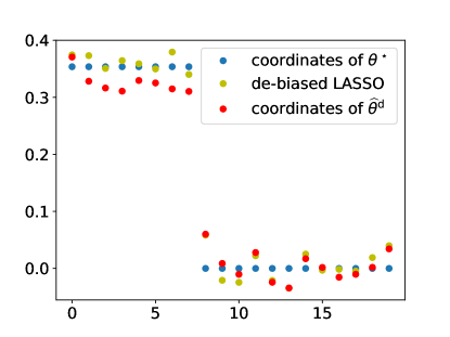
Figure 4: Comparison of our de-biased estimator and oracle de-biased LASSO estimator

H.1.3 Time series analysis

In our linear regression simulation, we generate i.i.d. random explanatory variables, and the observation noise is a 0-mean moving average (MA) process independent of the explanatory variables.

For the linear model

$$y_{i}=\langle x_{i},\theta^{\star}\rangle+\epsilon_{i},$$

$x_{i}\in\mathbb{R}^{20}$ are i.i.d. samples generated from $\mathcal{N}\left([1,1,\dots,1]^{\top}/\sqrt{k},I\right)$ , and $\epsilon_{i}$ is a 0-mean moving average process

$$\epsilon_{i}=0.6\cdot z_{i}+0.8\cdot z_{i-1},$$

where $z_{i}$ are i.i.d. $\mathcal{N}(0,0.7^{2})$.

We ran 100 simulations, with each time series containing 200 samples. For our approximate Newton statistical inference procedure (Algorithm 5), average 95% confidence interval (coverage, length) is (0.929, 0.145), and it matches our theory.

H.2 Real data

H.2.1 Neural network adversarial attack detection

The adversarial perturbation used in our experiments is shown in Figure 7. It is generated using the fast gradient sign method [GSS14] Figure 5 shows images in a “Shirt” example. Figure 6 shows images in a “T-shirt/top” example.

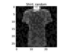
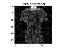
Figure 5: “Shirt” example

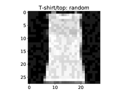
Figure 6: “T-shirt/top” example

Figure 7: Adversarial perturbation generated using the fast gradient sign method [GSS14]

H.2.2 High dimensional linear regression

For both experiments, the hyper-parameters are chosen based on the results in Section 3, where we estimate the true parameter’s $\ell_{1}$ norm $\|\theta^{\star}\|_{1}$ and noise level $\sigma$ by vanilla LASSO with cross validation, using the LASSO solution’s $\ell_{1}$ norm and LASSO residuals’ 2^nd moment’s square root. The covariance threshold is chosen so that it minimizes the thresholded covariance’s condition number.

HIV drug resistance mutations dataset.

We apply our high dimensional inference procedure to the dataset in [RTW⁺06] to detect mutations related to HIV drug resistance. Our procedure is able to detect verified mutations in an expert dataset [JBVC⁺05], when we control the family-wise error rate (FWER) at $0.05$.

Drug		Mutations
PI	APV	10F
	ATV	33F, 43T, 84V
	IDV	48V, 84A
	LPV	46I
	NFV	46L
	RTV	10I, 54V
	SQV	20R, 84V
NRTI	3TC	184V
	ABC	41L
	AZT	41L, 210W
	D4T	41L, 215Y
	DDI	62V, 151M
	TDF	41L, 75M
NNRTI	DLV	228R
	EFV	74V, 103N
	NVP	103N, 181C

Table 4: HIV drug resistance related mutations detected by our high dimensional inference procedure

Riboflavin (vitamin B2) production rate data set.

For the vanilla LASSO estimate on the high-throughput genomic data set concerning riboflavin (vitamin B2) production rate [BKM14], we set $\lambda=0.021864$. Figure 8, and we see that our point estimate is similar to the vanilla LASSO point estimate.

For statistical inference, in our method, we compute p-values using two-sided Z-test. Adjusting FWER to 5% signifi-cance level, our method does not find any significant gene. [JM14, BKM14] report that [Büh13] also does not find any significant gene, whereas [MMB09] finds one significant gene (YXLD-at), and [JM14] finds two significant genes (YXLD-at and YXLE-at). This indicates that our method is more conservative than [JM14, MMB09].

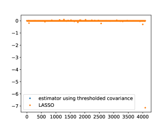
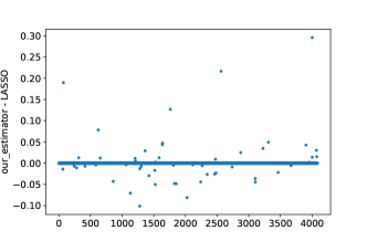
Figure 8: Comparison of our high dimensional linear regression point estimate with the vanilla LASSO estimate

H.2.3 Time series analysis

Using monthly equities returns data from [FP14], we use our approximate Newton statistical inference procedure to show that the correlation between US equities market returns and non-US global equities market returns is statistically significant, which validates the capital asset pricing model (CAPM) [Sha64, Lin65, FF04].

We regress monthly US equities market returns from 1995 to 2018 against other countries’ equities market returns, and each country’s coefficient and its 95% confidence interval is shown in Figure 9. And we observe that the US market is highly positively correlated with Canada and other advanced economies such as Germany and UK.

Figure 9: Exposure of US equities market to equities markets of other countries

References

• [ABH17] Naman Agarwal, Brian Bullins, and Elad Hazan. Second-order stochastic optimization for machine learning in linear time. The Journal of Machine Learning Research, 18(1):4148–4187, 2017.
• [AFM17] Yves F. Atchadé, Gersende Fort, and Eric Moulines. On perturbed proximal gradient algorithms. J. Mach. Learn. Res, 18(1):310–342, 2017.
• [Ama98] Shun-Ichi Amari. Natural gradient works efficiently in learning. Neural computation, 10(2):251–276, 1998.
• [ANW10] Alekh Agarwal, Sahand Negahban, and Martin Wainwright. Fast global convergence rates of gradient methods for high-dimensional statistical recovery. In Advances in Neural Information Processing Systems, pages 37–45, 2010.
• [ANW12] Alekh Agarwal, Sahand Negahban, and Martin J. Wainwright. Stochastic optimization and sparse statistical recovery: Optimal algorithms for high dimensions. In Advances in Neural Information Processing Systems, pages 1538–1546, 2012.
• [BBMS13] Jennifer Bender, Remy Briand, Dimitris Melas, and Raman Subramanian. Foundations of factor investing. 2013.
• [Ber91] Ernst Berndt. The practice of econometrics: classic and contemporary. Addison Wesley Publishing Company, 1991.
• [BHV14] Vineeth Balasubramanian, Shen-Shyang Ho, and Vladimir Vovk. Conformal prediction for reliable machine learning: theory, adaptations and applications. Newnes, 2014.
• [BJ16] Ronen Basri and David Jacobs. Efficient representation of low-dimensional manifolds using deep networks. arXiv preprint arXiv:1602.04723, 2016.
• [BKM14] Peter Bühlmann, Markus Kalisch, and Lukas Meier. High-dimensional statistics with a view toward applications in biology. Annual Review of Statistics and Its Application, 1:255–278, 2014.
• [BL08] Peter Bickel and Elizaveta Levina. Covariance regularization by thresholding. The Annals of Statistics, pages 2577–2604, 2008.
• [Bon36] C. Bonferroni. Teoria statistica delle classi e calcolo delle probabilita. Pubblicazioni del R Istituto Superiore di Scienze Economiche e Commericiali di Firenze, 8:3–62, 1936.
• [BRT09] Peter Bickel, Ya’acov Ritov, and Alexandre Tsybakov. Simultaneous analysis of Lasso and Dantzig selector. The Annals of Statistics, pages 1705–1732, 2009.
• [Bub15] Sébastien Bubeck. Convex optimization: Algorithms and complexity. Foundations and Trends in Machine Learning, 8(3-4):231–357, 2015.
• [Büh02] Peter Bühlmann. Bootstraps for time series. Statistical science, pages 52–72, 2002.
• [Büh13] Peter Bühlmann. Statistical significance in high-dimensional linear models. Bernoulli, 19(4):1212–1242, 2013.
• [BvdG11] Peter Bühlmann and Sara van de Geer. Statistics for high-dimensional data: methods, theory and applications. Springer Science & Business Media, 2011.
• [Car86] Edward Carlstein. The use of subseries values for estimating the variance of a general statistic from a stationary sequence. The Annals of Statistics, 14(3):1171–1179, 1986.
• [CFJL18] Emmanuel Candes, Yingying Fan, Lucas Janson, and Jinchi Lv. Panning for gold:‘model-x’knockoffs for high dimensional controlled variable selection. Journal of the Royal Statistical Society: Series B (Statistical Methodology), 80(3):551–577, 2018.
• [CLTZ16] Xi Chen, Jason Lee, Xin Tong, and Yichen Zhang. Statistical inference for model parameters in stochastic gradient descent. arXiv preprint arXiv:1610.08637, 2016.
• [CM16] Charles Chui and Hrushikesh Narhar Mhaskar. Deep nets for local manifold learning. arXiv preprint arXiv:1607.07110, 2016.
• [CZ12] Tony Cai and Harrison Zhou. Optimal rates of convergence for sparse covariance matrix estimation. The Annals of Statistics, pages 2389–2420, 2012.
• [DDB17] Aymeric Dieuleveut, Alain Durmus, and Francis Bach. Bridging the Gap between Constant Step Size Stochastic Gradient Descent and Markov Chains. arXiv preprint arXiv:1707.06386, 2017.
• [DH97] Anthony Christopher Davison and David Victor Hinkley. Bootstrap methods and their application. Cambridge University Press, 1997.
• [Dip08a] Jürgen Dippon. Asymptotic expansions of the Robbins-Monro process. Mathematical Methods of Statistics, 17(2):138–145, 2008.
• [Dip08b] Jürgen Dippon. Edgeworth expansions for stochastic approximation theory. Mathematical Methods of Statistics, 17(1):44–65, 2008.
• [DK98] John Driscoll and Aart Kraay. Consistent covariance matrix estimation with spatially dependent panel data. Review of Economics and Statistics, 80(4):549–560, 1998.
• [DLH16] Hadi Daneshmand, Aurelien Lucchi, and Thomas Hofmann. Starting small-learning with adaptive sample sizes. In International conference on machine learning, pages 1463–1471, 2016.
• [Edg08] Francis Ysidro Edgeworth. On the probable errors of frequency-constants. Journal of the Royal Statistical Society, 71(2):381–397, 1908.
• [EH16] B. Efron and T. Hastie. Computer age statistical inference. Cambridge University Press, 2016.
• [ET94] Bradley Efron and Robert J. Tibshirani. An introduction to the bootstrap. CRC press, 1994.
• [FF04] Eugene F. Fama and Kenneth R. French. The capital asset pricing model: Theory and evidence. Journal of economic perspectives, 18(3):25–46, 2004.
• [FGLS18] Jianqing Fan, Wenyan Gong, Chris Junchi Li, and Qiang Sun. Statistical sparse online regression: A diffusion approximation perspective. In International Conference on Artificial Intelligence and Statistics, pages 1017–1026, 2018.
• [FHT01] J. Friedman, T. Hastie, and R. Tibshirani. The elements of statistical learning, volume 1. Springer series in statistics New York, 2001.
• [FP14] Andrea Frazzini and Lasse Heje Pedersen. Betting against beta. Journal of Financial Economics, 111(1):1–25, 2014.
• [FXY17] Yixin Fang, Jinfeng Xu, and Lei Yang. On Scalable Inference with Stochastic Gradient Descent. arXiv preprint arXiv:1707.00192, 2017.
• [GP17] Sébastien Gadat and Fabien Panloup. Optimal non-asymptotic bound of the Ruppert-Polyak averaging without strong convexity. arXiv preprint arXiv:1709.03342, 2017.
• [GSS14] Ian J. Goodfellow, Jonathon Shlens, and Christian Szegedy. Explaining and harnessing adversarial examples. arXiv preprint arXiv:1412.6572, 2014.
• [HAV+15] Reza Harikandeh, Mohamed Osama Ahmed, Alim Virani, Mark Schmidt, Jakub Konecny, and Scott Sallinen. StopWasting My Gradients: Practical SVRG. In Advances in Neural Information Processing Systems 28, pages 2251–2259, 2015.
• [Hoe07] Daniel Hoechle. Robust standard errors for panel regressions with cross-sectional dependence. Stata Journal, 7(3):281–312, 2007.
• [Hub67] Peter Huber. The behavior of maximum likelihood estimates under nonstandard conditions. In Proceedings of the fifth Berkeley symposium on Mathematical Statistics and Probability, pages 221–233, Berkeley, CA, 1967. University of California Press.
• [JBVC+05] Victoria A Johnson, Francoise Brun-Vezinet, Bonaventura Clotet, Brian Conway, Daniel R. Kuritzkes, Deenan Pillay, Jonathan Schapiro, Amalio Telenti, and Douglas Richman. Update of the drug resistance mutations in HIV-1: 2005. Topics in HIV medicine: a publication of the International AIDS Society, USA, 13(1):51–57, 2005.
• [JD11] Jessie Jeng and John Daye. Sparse covariance thresholding for high-dimensional variable selection. Statistica Sinica, pages 625–657, 2011.
• [JJ18] Adel Javanmard and Hamid Javadi. False Discovery Rate Control via Debiased Lasso. arXiv preprint arXiv:1803.04464, 2018.
• [JM14] Adel Javanmard and Andrea Montanari. Confidence intervals and hypothesis testing for high-dimensional regression. Journal of Machine Learning Research, 15(1):2869–2909, 2014.
• [JM15] Adel Javanmard and Andrea Montanari. De-biasing the Lasso: Optimal sample size for Gaussian designs. arXiv preprint arXiv:1508.02757, 2015.
• [JZ13] Rie Johnson and Tong Zhang. Accelerating stochastic gradient descent using predictive variance reduction. In Advances in neural information processing systems, pages 315–323, 2013.
• [KD99] Aart Kraay and John Driscoll. Spatial Correlations in Panel Data. The World Bank, 1999.
• [KL12] Jens-Peter Kreiss and Soumendra Nath Lahiri. Bootstrap methods for time series. In Handbook of statistics, volume 30, pages 3–26. Elsevier, 2012.
• [KTSJ14] Ariel Kleiner, Ameet Talwalkar, Purnamrita Sarkar, and Michael Jordan. A scalable bootstrap for massive data. Journal of the Royal Statistical Society: Series B (Statistical Methodology), 76(4):795–816, 2014.
• [Kun89] Hans Kunsch. The jackknife and the bootstrap for general stationary observations. The annals of Statistics, pages 1217–1241, 1989.
• [Lah13] Soumendra Nath Lahiri. Resampling methods for dependent data. Springer Science & Business Media, 2013.
• [LH15] Ilya Loshchilov and Frank Hutter. Online batch selection for faster training of neural networks. arXiv preprint arXiv:1511.06343, 2015.
• [Lin65] John Lintner. The valuation of risk assets and the selection of risky investments in stock portfolios and capital budgets. The Review of Economics and Statistics, pages 13–37, 1965.
• [LLKC18] Tianyang Li, Liu Liu, Anastasios Kyrillidis, and Constantine Caramanis. Statistical inference using SGD. In The Thirty-Second AAAI Conference on Artificial Intelligence (AAAI-18), 2018.
• [Loh17] Po-Ling Loh. Statistical consistency and asymptotic normality for high-dimensional robust $M$-estimators. The Annals of Statistics, 45(2):866–896, 2017.
• [LSS14] Jason Lee, Yuekai Sun, and Michael Saunders. Proximal Newton-type methods for minimizing composite functions. SIAM Journal on Optimization, 24(3):1420–1443, 2014.
• [LW17] Po-Ling Loh and Martin Wainwright. Support recovery without incoherence: A case for nonconvex regularization. The Annals of Statistics, 45(6):2455–2482, 2017.
• [MB11] Eric Moulines and Francis R. Bach. Non-asymptotic analysis of stochastic approximation algorithms for machine learning. In Advances in Neural Information Processing Systems, pages 451–459, 2011.
• [MMB09] Nicolai Meinshausen, Lukas Meier, and Peter Bühlmann. $p$-values for high-dimensional regression. Journal of the American Statistical Association, 104(488):1671–1681, 2009.
• [NRWY12] Sahand Negahban, Pradeep Ravikumar, Martin Wainwright, and Bin Yu. A Unified Framework for High-Dimensional Analysis of M-Estimators with Decomposable Regularizers. Statistical Science, pages 538–557, 2012.
• [NW86] Whitney Newey and Kenneth West. A simple, positive semi-definite, heteroskedasticity and autocorrelation consistent covariance matrix. National Bureau of Economic Research Cambridge, Mass., USA, 1986.
• [NW94] Whitney Newey and Kenneth West. Automatic lag selection in covariance matrix estimation. The Review of Economic Studies, 61(4):631–653, 1994.
• [PJ92] Boris Polyak and Anatoli Juditsky. Acceleration of stochastic approximation by averaging. SIAM Journal on Control and Optimization, 30(4):838–855, 1992.
• [PR92] Dimitris Politis and Joseph Romano. A circular block-resampling procedure for stationary data. Exploring the limits of bootstrap, pages 263–270, 1992.
• [PR94] Dimitris Politis and Joseph Romano. The stationary bootstrap. Journal of the American Statistical association, 89(428):1303–1313, 1994.
• [PRW12] D. N. Politis, J. P. Romano, and M. Wolf. Subsampling. Springer Series in Statistics. Springer New York, 2012.
• [RLZ09] Adam Rothman, Elizaveta Levina, and Ji Zhu. Generalized thresholding of large covariance matrices. Journal of the American Statistical Association, 104(485):177–186, 2009.
• [RM73] Barr Rosenberg and Walt McKibben. The prediction of systematic and specific risk in common stocks. Journal of Financial and Quantitative Analysis, 8(2):317–333, 1973.
• [RTW+06] Soo-Yon Rhee, Jonathan Taylor, Gauhar Wadhera, Asa Ben-Hur, Douglas L. Brutlag, and Robert W. Shafer. Genotypic predictors of human immunodeficiency virus type 1 drug resistance. Proceedings of the National Academy of Sciences, 103(46):17355–17360, 2006.
• [Rup88] David Ruppert. Efficient estimations from a slowly convergent Robbins-Monro process. Technical report, Cornell University Operations Research and Industrial Engineering, 1988.
• [RWY11] Garvesh Raskutti, Martin Wainwright, and Bin Yu. Minimax rates of estimation for high-dimensional linear regression over $\ell_{q}$-balls. IEEE transactions on information theory, 57(10):6976–6994, 2011.
• [SEG+17] Levent Sagun, Utku Evci, V. Ugur Guney, Yann Dauphin, and Leon Bottou. Empirical Analysis of the Hessian of Over-Parametrized Neural Networks. arXiv preprint arXiv:1706.04454, 2017.
• [Sha64] William F. Sharpe. Capital asset prices: A theory of market equilibrium under conditions of risk. The journal of finance, 19(3):425–442, 1964.
• [SS11] Robert Shumway and David Stoffer. Time series regression and exploratory data analysis. In Time series analysis and its applications, pages 47–82. Springer, 2011.
• [SV08] Glenn Shafer and Vladimir Vovk. A tutorial on conformal prediction. Journal of Machine Learning Research, 9(Mar):371–421, 2008.
• [SZ18] Weijie Su and Yuancheng Zhu. Statistical Inference for Online Learning and Stochastic Approximation via Hierarchical Incremental Gradient Descent. arXiv preprint arXiv:1802.04876, 2018.
• [TA17] Panos Toulis and Edoardo M. Airoldi. Asymptotic and finite-sample properties of estimators based on stochastic gradients. The Annals of Statistics, 45(4):1694–1727, 2017.
• [Tro15] Joel Tropp. An introduction to matrix concentration inequalities. Foundations and Trends in Machine Learning, 8(1-2):1–230, 2015.
• [TRVB06] F. Tuerlinckx, F. Rijmen, G. Verbeke, and P. Boeck. Statistical inference in generalized linear mixed models: A review. British Journal of Mathematical and Statistical Psychology, 59(2):225–255, 2006.
• [TWH15] R. Tibshirani, M. Wainwright, and T. Hastie. Statistical learning with sparsity: the lasso and generalizations. Chapman and Hall/CRC, 2015.
• [Var75] James Varah. A lower bound for the smallest singular value of a matrix. Linear Algebra and its Applications, 11(1):3–5, 1975.
• [vdGBRD14] Sara van de Geer, Peter Bühlmann, Ya’acov Ritov, and Ruben Dezeure. On asymptotically optimal confidence regions and tests for high-dimensional models. The Annals of Statistics, 42(3):1166–1202, 2014.
• [vdV98] Aad W. van der Vaart. Asymptotic statistics. Cambridge University Press, 1998.
• [VGS05] Vladimir Vovk, Alexander Gammerman, and Glenn Shafer. Algorithmic learning in a random world: conformal prediction. Springer, 2005.
• [Wai09] Martin Wainwright. Sharp thresholds for High-Dimensional and noisy sparsity recovery using $\ell_{1}$-Constrained Quadratic Programming (Lasso). IEEE transactions on information theory, 55(5):2183–2202, 2009.
• [Wai17] Martin J. Wainwright. High-Dimensional Statistics: A Non-Asymptotic Viewpoint. To appear, 2017.
• [Was13] Larry Wasserman. All of statistics: a concise course in statistical inference. Springer Science & Business Media, 2013.
• [Whi80] Halbert White. A heteroskedasticity-consistent covariance matrix estimator and a direct test for heteroskedasticity. Econometrica: Journal of the Econometric Society, pages 817–838, 1980.
• [XRV17] Han Xiao, Kashif Rasul, and Roland Vollgraf. Fashion-MNIST: a Novel Image Dataset for Benchmarking Machine Learning Algorithms. arXiv preprint arXiv:1708.07747, 2017.
• [XZ14] Lin Xiao and Tong Zhang. A proximal stochastic gradient method with progressive variance reduction. SIAM Journal on Optimization, 24(4):2057–2075, 2014.
• [YLR14] Eunho Yang, Aurelie Lozano, and Pradeep Ravikumar. Elementary estimators for high-dimensional linear regression. In International Conference on Machine Learning, pages 388–396, 2014.
• [ZZ14] Cun-Hui Zhang and Stephanie Zhang. Confidence intervals for low dimensional parameters in high dimensional linear models. Journal of the Royal Statistical Society: Series B (Statistical Methodology), 76(1):217–242, 2014.