UNSUPERVISED DOMAIN ADAPTATION USING REGULARIZED HYPER-GRAPH MATCHING

Abstract

Domain adaptation (DA) addresses the real-world image classification problem of discrepancy between training (source) and testing (target) data distributions. We propose an unsupervised DA method that considers the presence of only unlabelled data in the target domain. Our approach centers on finding matches between samples of the source and target domains. The matches are obtained by treating the source and target domains as hyper-graphs and carrying out a class-regularized hyper-graph matching using first-, second- and third-order similarities between the graphs. We have also developed a computationally efficient algorithm by initially selecting a subset of the samples to construct a graph and then developing a customized optimization routine for graph-matching based on Conditional Gradient and Alternating Direction Multiplier Method. This allows the proposed method to be used widely. We also performed a set of experiments on standard object recognition datasets to validate the effectiveness of our framework over previous approaches.

Index Terms—  Domain Adaptation, Transfer Learning, Hyper-Graph Matching, Object Recognition

1 Introduction

The assumption that test data is drawn from the same distribution as the training data is rarely encountered in real-world, machine learning problems. For example, consider a recognition system that distinguishes between a cat and a dog, and has been trained using labelled samples of the type shown in Fig. 1(a). The same system when used to test in a different domain such as on the side images of cats and dogs (see Fig. 1(b)) would fail miserably. This is because the recognition system has developed a bias in only distinguishing between the face of a dog and a cat and not their side images. Domain adaptation (DA) aims to mitigate this dataset bias [1], where different datasets have their own unique properties. In this work, we consider unsupervised domain adaptation (UDA) where we have labelled source domain data and only unlabelled target domain data.

Most previous UDA methods can be broadly classified into two categories. Instance Re-weighting was one of the early methods, where it was assumed that conditional distributions were shared between the two domains. The instance re-weighting involved estimating the ratio between the likelihoods of being a source example or a target example to compute the weight of an instance. This was done by estimating the likelihoods independently [2] or by approximating the ratio between the densities [3, 4]. One of the most popular measures used to weigh data instances was the Maximum Mean Discrepancy (MMD) [5], which computed the divergence between the data distributions in the two domains.

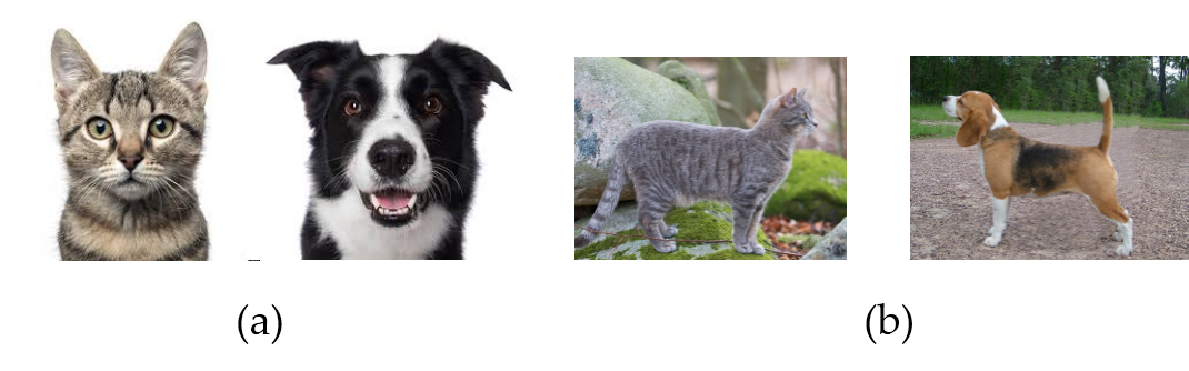
Fig. 1: Source (a) and Target (b) domain has front and side views respectively.

The Feature Transfer category consists of the bulk of the UDA methods. Well known feature transfer methods include the Geodesic Flow Sampling (GFS) [6, 7] and the Geodesic Flow Kernel (GFK) [8, 9], where the domains are embedded in $d$-dimensional linear subspaces that can be seen as points on the Grassman manifold. The Subspace Alignment (SA) [10] learns an alignment between the source subspace obtained by Principal Component Analysis (PCA) and the target PCA subspace, where the PCA dimensions are selected by minimizing the Bregman divergence between the subspaces. Similarly, the linear Correlation Alignment (CORAL) [11] algorithm minimizes the domain shift using the covariance of the source and target distributions. Transfer Component Analysis (TCA) [12] discovers common latent features having the same marginal distribution across the source and target domains. The Optimal Transport for Domain Adaptation  [13], considers a local transportation plan for each source example to be mapped close to the target samples. Our approach is similar to [13] in the sense that it considers local sample-to-sample matching and this generally results in better performance than global methods because it considers the effect of each and every sample in the dataset explicitly. In [13], they considered a first-order, point-wise unary cost between each source and target sample. Our approach develops a framework that exploit higher-order relations along with these unary relations. Such higher order relations provide additional geometric and structural information about the data beyond the unary point-wise relations. Hence, we expect higher order matching between source and target domains to yield better domain adaptation. In fact, a higher-order graph matching problem has been previously used for finding feature correspondences in images [14, 15] through a tensor-based formulation but has not been applied to domain adaptation.

In that sense, our contributions are in the following ways: (1) A mathematical framework using all the first-, second- and third-order relations to match the source- and target-domain samples along with a regularization using labels of the source-domain data. (2) Computationally efficient method of obtaining the solution of the optimization problem by solving a series of sub-problems using Alternating Direction Multiplier Method (ADMM). Moreover, we perform an initial clustering to select the most relevant instances and thus reduce the number of data points to be used in the optimization approach. (3) Experimental evaluation on an object recognition dataset with analysis of the effect of each cost term. Fig. 2 shows the intuition of our method in a two-dimensional setting.

2 PROPOSED DOMAIN-ADAPTATION METHOD

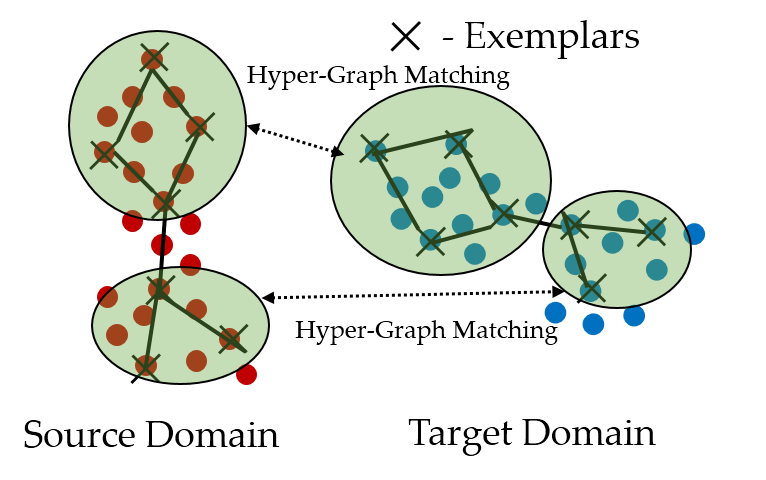
Fig. 2: Our approach involves extracting exemplars from both source and target domain. Hyper-graphs are constructed from those exemplars followed by matching.

2.1 Problem formulation

For unsupervised domain adaptation (UDA), we have the source domain data matrix ${\bf X}^{s}\in\mathbb{R}^{n_{s}\times d}$, vector of source domain data labels ${\bf y}^{s}\in\mathbb{R}^{n_{s}}$ and the target domain data matrix ${\bf X}^{t}\in\mathbb{R}^{n_{t}\times d}$. Here, $n_{s}$ and $n_{t}$ are the number of source and target samples respectively, and $d$ is the dimension of the feature space. The labels in ${\bf y}^{s}$ range in $\{1,2,\cdots,C\}$. Both the domains share the same $C$ number of classes. For the purpose of UDA, we transform the source domain data close to the target domain data such that a classifier trained on the transformed source domain predicts well on the target instances.

2.1.1 Finding Exemplars

In our proposed method, we initially perform clustering to extract the set of exemplars, which is a representative subset of the original source and target domain dataset. This clustering is required to increase the computational efficiency of our hyper-graph matching method. We use Affinity Propagation (AP) [16] to extract the exemplars. AP is an efficient clustering algorithm that uses message passing between data-points. The algorithm requires the similarity matrix ${\bf S}$ of a dataset as the input. Here, $[{\bf S}]_{ij}=-||{\bf x}_{i}-{\bf x}_{j}||^{2},i\neq j$ and $[{\bf S}]_{ii}$ is the preference of sample ${\bf x}_{i}$ to be an exemplar and is set to the same value of $p$ for all instances. $p$ controls the number of exemplars obtained. For low values of $p$ we obtain less exemplars while for large values of $p$ we obtain more exemplars. To obtain a desired number of exemplars, a bisection method that adjusts $p$ iteratively is used. For our purpose, we set $\eta$ to be the desired fraction of exemplars for both the source and the target domain dataset. Thus, as an output of the AP algorithm, we would obtain the exemplar source and target domain matrix ${\bf X}^{\prime s}\in\mathbb{R}^{n^{\prime}_{s}\times d}$ and ${\bf X}^{\prime t}\in\mathbb{R}^{n^{\prime}_{t}\times d}$, respectively, where $n^{\prime}_{s}\approx\eta n_{s}$, $n^{\prime}_{t}\approx\eta n_{t}$. However, to keep up with the notation, from now onwards in the paper we would denote ${\bf X}^{s}$, ${\bf X}^{t}$ as the exemplar source and target datasets and $n_{s}$ and $n_{t}$ as the number of source and target exemplars.

2.1.2 Hyper-Graph Matching

To carry out hyper-graph matching between the source and target exemplars, we consider all first-, second- and third-order matching between the source and target exemplars. We do not use just the higher order matching because the source and target hyper-graphs will be far from isomorphic and using only the structural information will produce misleading results. On the contrary for registration between similarly shaped objects [14], using only higher order matching produces excellent results.

We seek to find a matching matrix ${\bf C}\in\mathbb{R}^{n_{s}\times n_{t}}$, where $[{\bf C}]_{ij}$ is the measure of correspondence between source exemplar $i$ and target exemplar $j$. For the first-order matching, we would like exemplars in the source domain to be close to similar exemplars in the target domain. Since the operation ${\bf C}{\bf X}^{t}$ rearranges the target exemplars, we would like the re-arranged target exemplars ${\bf C}{\bf X}^{t}$ to be close to ${\bf X}^{s}$. Thus, to enable first-order matching, we would like to minimize the normalized term $f_{1}({\bf C})=||{\bf C}{\bf X}^{t}-{\bf X}^{s}||^{2}_{\mathcal{F}}/(n_{s}d)$, where $||\cdot||_{\mathcal{F}}$ is the Frobenius norm.

For the second-order matching, we would like source exemplar pairs to match with similar target exemplar pairs. This is carried out by initially constructing a source and a target adjacency matrix with source and target exemplars as graph nodes. If ${\bf D}^{s}$ and ${\bf D}^{t}$ are source and target adjacency matrices, then $[{\bf D}^{s}]_{ij}=\text{exp}({-\frac{||{\bf x}^{s}_{i}-{\bf x}^{s}_{j}||^{2}_{2}}{{\sigma}_{s}^{2}}})$, $[{\bf D}^{t}]_{ij}=\text{exp}({-\frac{||{\bf x}^{t}_{i}-{\bf x}^{t}_{j}||^{2}_{2}}{{\sigma}_{t}^{2}}})$ for $i\neq j$ and $[{\bf D}^{s}]_{ii}=[{\bf D}^{t}]_{ii}=0$. ${\sigma}_{s}$ and ${\sigma}_{t}$ can be found heuristically as the mean sample-to-sample pairwise distance in the source and target domains, respectively. For the second-order similarity, we want the row re-arranged target domain adjacency matrix ${\bf C}{\bf D}^{t}$ to be close to the column-rearranged source domain adjacency matrix ${\bf D}^{s}{\bf C}$. Taking into consideration the difference in the numbers of source and target exemplars $n_{s}$ and $n_{t}$, second-order graph matching implies minimizing the term $f_{2}({\bf C})=||{\bf C}{\bf D}^{t}-r{\bf D}^{s}{\bf C}||^{2}_{\mathcal{F}}$, where $r=\frac{n_{t}}{n_{s}}$ is a correction factor.

For the third-order matching problem, we use the tensor based cost term [14]. In that paper, they try to maximize the cost term $f_{3}({\bf C})={\bf H}\otimes_{1}{\bf c}\otimes_{2}{\bf c}\otimes_{3}{\bf c}$, where ${\bf H}\in\mathbb{R}^{{n_{s}n_{t}}\times{n_{s}n_{t}}\times{n_{s}n_{t}}}$ is a third-order tensor and the index $k$ in $\otimes_{k}$ indicates tensor multiplication on the $k^{th}$ dimension and ${\bf c}\in\mathbb{R}^{n_{s}n_{t}}$ is the vectorized matching matrix ${\bf C}$. Here, $[{\bf H}]_{ijk}=\text{exp}(-\gamma||f_{i_{s},j_{s},k_{s}}-f_{i_{t},j_{t},k_{t}}||^{2})$. If ${\bf c}_{i}$ is the matching variable for the samples ${\bf x}^{s}_{i}$ and ${\bf x}^{t}_{i}$, ${\bf c}_{j}$ for the samples ${\bf x}^{s}_{j}$ and ${\bf x}^{t}_{j}$ and ${\bf c}_{k}$ for the samples ${\bf x}^{s}_{k}$ and ${\bf x}^{t}_{k}$, then $f_{i_{s},j_{s},k_{s}}$ is the feature consisting of the sine of the angles of the triangle formed by the data points ${\bf x}^{s}_{i},{\bf x}^{s}_{j}$ and ${\bf x}^{s}_{k}$ and $f_{i_{t},j_{t},k_{t}}$ consisting of the sine of the angles of the triangle formed by the data points ${\bf x}^{t}_{i},{\bf x}^{t}_{j}$ and ${\bf x}^{t}_{k}$. $\gamma$ is calculated from the mean pairwise squared distance between the features.

In addition to the graph-matching terms, we add a class-based regularization. The group-lasso regularizer [17] $\ell_{2}-\ell_{1}$ norm term is equal to $f_{g}({\bf C})=\sum_{j}\sum_{c}||[{\bf C}]_{\mathcal{I}_{c}j}||_{2}$, where $||\cdot||_{2}$ is the $\ell_{2}$ norm and $\mathcal{I}_{c}$ contains the indices of rows of ${\bf C}$ corresponding to the source-domain samples of class $c$. In other words, $[{\bf C}]_{\mathcal{I}_{c}j}$ is a vector consisting of elements $[{\bf C}]_{ij}$, where $i^{th}$ source sample belongs to class $c$ and the $j^{th}$ sample is in the target domain. Minimizing this group-lasso term ensures that a target-domain sample only corresponds to the source-domain samples that have the same label.

In the case of $n_{t}=n_{s}$, we have one-to-one matching between each source sample and each target sample. However, for the case $n_{t}\neq n_{s}$, we must allow multiple correspondences. Accordingly, if the constraint ${\bf C}\mathbf{1}_{n_{t}}=\mathbf{1}_{n_{s}}$ ($\mathbf{1}_{n}$ is a $n\times 1$ vector of ones) implies that the sum of the correspondences of all the target samples to each source sample is one, then the second equality constraint ${\bf C}^{T}\mathbf{1}_{n_{s}}=\frac{n_{s}}{n_{t}}\mathbf{1}_{n_{t}}$ implies that the sum of correspondences of all the source samples to each target sample should increase proportionately by $\frac{n_{s}}{n_{t}}$ to allow for the multiple correspondences. Hence, the overall optimization problem becomes

Problem UDA

$$\min\limits_{{\bf C}}f({\bf C})~{} =~{}\frac{1}{(n_{s}d)}||{\bf C}{\bf X}^{t}-{\bf X}^{s}||^{2}_{\mathcal{F}}+\lambda_{2}||{\bf C}{\bf D}^{t}-r{\bf D}^{s}{\bf C}||^{2}_{\mathcal{F}}$$

$$-\lambda_{3}{\bf H}\otimes_{1}{\bf c}\otimes_{2}{\bf c}\otimes_{3}{\bf c}+\lambda_{g}\sum_{j}\sum_{c}||[{\bf C}]_{\mathcal{I}_{c}j}||_{2}$$ (1)

$${\rm such~{}that} ~{}{\bf C}\geq{\bf 0},~{}{\bf C}\mathbf{1}_{n_{t}}=\mathbf{1}_{n_{s}},~{}{\rm and}~{}{\bf C}^{T}\mathbf{1}_{n_{s}}=(\frac{n_{s}}{n_{t}})\mathbf{1}_{n_{t}}.$$

2.2 Problem Solution

Problem UDA can be solved quickly using second-order methods but has memory and computational issues related to storing the Hessian ($O(n_{s}^{2}n_{t}^{2})$). Hence, first-order methods, specially conditional gradient method (CG) [18] can be used to solve the problem. The CG method maintains the desirable structure of the solution such as sparsity required of ${\bf C}$ by solving the successive linear minimization sub-problems over the constraint set [19]. The linear programming (LP) subproblem required to be solved is minimizing $\mathbf{Tr}({\bf G}^{T}{\bf C})$ ,${\bf C}\geq\mathbf{0},{\bf C}\mathbf{1}_{n_{t}}=\mathbf{1}_{n_{s}},{\bf C}^{T}\mathbf{1}_{n_{s}}=\frac{n_{s}}{n_{t}}\mathbf{1}_{n_{t}}$, where ${\bf G}$ is the gradient of the function $f$ in Problem UDA and $\mathbf{Tr}(\cdot)$ is the trace operation. The gradient of each cost term can be derived as

$$\nabla f_{1}({\bf C}) =2({\bf C}{\bf X}^{t}-{\bf X}^{s}){\bf X}^{tT}/(n_{s}d),$$

$$\nabla f_{2}({\bf C}) =~{}2({\bf C}{\bf D}^{t}{\bf D}^{tT}-r{\bf D}^{s}{\bf C}{\bf D}^{tT}-r{\bf D}^{sT}{\bf C}{\bf D}^{t}+r^{2}{\bf D}^{sT}{\bf D}^{s}{\bf C})~{},~{}$$

$$\nabla f_{3}({\bf C}) =(\mathbf{[}{\bf H}\otimes_{1}{\bf c}\otimes_{2}{\bf c}+{\bf H}\otimes_{1}{\bf c}\otimes_{3}{\bf c}+{\bf H}\otimes_{2}{\bf c}\otimes_{3}{\bf c}\mathbf{]})~{}~{}$$

$$\frac{\partial f_{g}}{\partial[{\bf C}]_{ij}} =\frac{[{\bf C}]_{ij}}{||[{\bf C}]_{\mathcal{I}_{c}(i)j}||_{2}}\cdot\delta(||[{\bf C}]_{\mathcal{I}_{c}(i)j}||_{2}\neq 0)$$

Here $[\cdot]$ operator on tensor term reshapes a vector into matrix of size $n_{s}\times n_{t}$. $c(i)$ is the class of the $i^{th}$ source sample. $\delta(\cdot)$ is an indicator function which is 1 if the argument is true and 0 otherwise. Thus, after obtaining the gradient ${\bf G}=\nabla f(C)=\nabla f_{1}(C)+\lambda_{2}\nabla f_{2}(C)-\lambda_{3}\nabla f_{3}(C)+\lambda_{g}\nabla f_{g}(C)$, we solve the linear minimization problem LP mentioned before using the consensus form of ADMM [20]. We let ${\bf a}=\mathbf{1}_{n_{s}}$ and ${\bf b}=\frac{n_{s}}{n_{t}}\mathbf{1}_{n_{t}}$. Using the consensus ADMM form, we reformulate LP as

$$\min \left\{g_{1}({\bf C}_{1})+g_{2}({\bf C}_{2})+g_{3}({\bf C}_{3})\right\}$$

such that $$\quad{\bf Z}={\bf C}_{1}={\bf C}_{2}={\bf C}_{3}$$

where $g_{1}({\bf C}_{1})=0.5\mathbf{Tr}({\bf G}^{T}{\bf C}_{1})+{I}({\bf C}_{1}\mathbf{1}_{n_{t}}={\bf a})$, $g_{2}({\bf C}_{2})=0.5\mathbf{Tr}({\bf G}^{T}{\bf C}_{2})+{I}({\bf C}_{2}^{T}\mathbf{1}_{n_{s}}={\bf b})$ and $g_{3}({\bf C}_{3})={I}({\bf C}_{3}\geq\mathbf{0})$. Here, $I(\cdot)$ is an indicator function which is 0 if argument is true and $\infty$ otherwise. $\mathbf{Z}$ is an intermediate variable to facilitate consensus ADMM. Accordingly, the ADMM updates will be as follows

$${\bf C}_{1}^{k+1}=\underset{{\bf C}_{1}\mathbf{1}_{n_{t}}={\bf a}}{\text{argmin}}(\mathbf{Tr}((0.5{\bf G}+{\bf Y}_{1}^{k})^{T}{\bf C}_{1})+\frac{\rho}{2}||{\bf C}_{1}-{\bf Z}^{k}||_{F}^{2})$$

$${\bf C}_{2}^{k+1}=\underset{{\bf C}_{2}^{T}\mathbf{1}_{n_{s}}={\bf b}}{\text{argmin}}(\mathbf{Tr}((0.5{\bf G}+{\bf Y}_{2}^{k})^{T}{\bf C}_{2})+\frac{\rho}{2}||{\bf C}_{2}-{\bf Z}^{k}||_{F}^{2})$$

$${\bf C}_{3}^{k+1}=\Pi_{\{{\bf C}|{\bf C}\geq\mathbf{0}\}}({\bf Z}^{k}-{\bf Y}_{3}^{k}),\quad{\bf Z}^{k+1}=\frac{1}{3}(\sum_{i}{\bf C}_{i}^{k+1})$$

$${\bf Y}_{i}^{k+1}={\bf Y}_{i}^{k}+{\bf C}_{i}^{k+1}-{\bf Z}^{k+1}\quad\forall i=1,2,3$$

Here ${\bf Y}_{i}$’s are dual variables. $\Pi$ is the projection operator. The penalty parameter is set $\rho=1$ without loss of generality since scaling $\rho$ is equivalent to scaling ${\bf G}$. Updates for ${\bf C}_{1}^{k+1}$ and ${\bf C}_{2}^{k+1}$ are solved using Lagrange multiplier to obtain

$${\bf C}_{1}^{k+1} ={\bf Z}^{k}-\frac{{\bf G}}{2}-{\bf Y}_{1}^{k}-\frac{1}{n_{t}}(({\bf Z}^{k}-\frac{{\bf G}}{2}-{\bf Y}_{1}^{k})\mathbf{1}_{n_{t}}-{\bf a})\mathbf{1}_{n_{t}}^{T},$$

$${\bf C}_{2}^{k+1} ={\bf Z}^{k}-\frac{{\bf G}}{2}-{\bf Y}_{2}^{k}-\frac{1}{n_{s}}\mathbf{1}_{n_{s}}(\mathbf{1}_{n_{s}}^{T}({\bf Z}^{k}-\frac{{\bf G}}{2}-{\bf Y}_{2}^{k})-{\bf b}^{T}),$$

$${\bf C}_{3}^{k+1} =\text{max}({\bf Z}^{k}-{\bf Y}_{3}^{k},\textbf{0})$$

The ADMM updates are repeated for a fixed few-hundred iterations and the optimum value of LP is set to final value of ${\bf Z}$. This would complete one iteration of CG. After completing several such iterations of CG, we can obtain the optimal value of ${\bf C}^{*}$. Using that, we can map the source domain data close to the target domain data using regression with ${\bf X}^{s}$ and ${\bf C}^{*}{\bf X}^{t}$ as the input and output data respectively. The whole procedure can be repeated for a number of times at the end of which the adapted source data is used to train a classifier to be tested on target domain data. The overall algorithm is given below in Algorithm 1.

Given : Source Labelled Data ${\bf X}^{s}$ and ${\bf y}^{s}$, and Target Unlabelled Data ${\bf X}^{t}$

Parameters : $\eta,\lambda_{2},\lambda_{3},\lambda_{g},N_{T}$

Initialize : $t_{o}=0$

Repeat

${\bf X}^{s},{\bf X}^{t}\leftarrow\mathbf{AP}({\bf X}^{s},{\bf X}^{t},\eta)$, (Affinity Propagation)

Initialize: ${\bf C}_{0}\in\mathcal{D}$, $t_{i}=1$

Repeat (Conditional Gradient)

 ${\bf G}=\nabla_{C}f({\bf C}_{0})$, ${\bf C}_{d}\leftarrow\text{ADMM}({\bf G},{\bf a}.{\bf b})$

 ${\bf C}_{1}={\bf C}_{0}+\alpha({\bf C}_{d}-{\bf C}_{0}),\quad\text{for}\quad\alpha=\frac{2}{t_{i}+2}$

 ${\bf C}_{0}={\bf C}_{1}$  and  $t_{i}=t_{i}+1$

Until Fixed Number of Iterations

${\bf C}^{*}={\bf C}_{0}$ and Regress ${\bf M}(\cdot)\quad\text{s.t.}\quad{\bf X}^{s}\xrightarrow[]{\textbf{M}}{\bf C}^{*}{\bf X}^{t}$

Map ${\bf X}^{s}\leftarrow{\bf M}({\bf X}^{s})$  and  $t_{o}=t_{o}+1$

Until $t_{o}=N_{T}$

Output : Adapted Source Data ${\bf X}^{s}$

Algorithm 1 UDA with Hyper-graph matching

2.3 Time and Space Complexity

The AP clustering algorithm has a time complexity of ($O(n_{s}^{2}+n_{t}^{2})$). The ADMM updates are linear in the number of variables ($O(\eta^{2}n_{s}n_{t})$) and they run for a fixed number of iterations. They are faster than interior point methods, which would result in cubic time-complexity in the number of variables. The overall time complexity will be multiplied by $N_{T}$. For the space complexity, the AP algorithm requires storing source and target similarity matrices of $O(n_{s}^{2}+n_{t}^{2})$. Graph adjacency matrices also require space complexity of $O(\eta^{2}n_{s}^{2}+\eta^{2}n_{t}^{2})$. For tensor storage, we use the sparse strategy [14] to obtain $O(m)$ space complexity, where $m$ is the number of non-zero entries and $m\propto\max(\eta n_{s},\eta n_{t})$

3 EXPERIMENTAL RESULTS

Table 1: Comparing different methods in terms of classification accuracy (%) of target data. Each task consists of source $\rightarrow$ target, where source and target represent any of the four domains: C(Caltech-256), A(Amazon), W(Webcam) and D(DSLR).

Method	C $\rightarrow$ A	C $\rightarrow$ W	C $\rightarrow$ D	A $\rightarrow$ C	A $\rightarrow$ W	A $\rightarrow$ D	W $\rightarrow$ C	W $\rightarrow$ A	W $\rightarrow$ D	D $\rightarrow$ C	D $\rightarrow$ A	D $\rightarrow$ W
NA	21.86	20.97	22.73	23.85	24.31	21.95	19.03	23.22	50.91	23.79	26.11	51.67
GFK	33.41	33.06	35.19	32.50	33.89	31.45	25.12	31.17	79.22	30.04	32.15	71.87
SA	34.12	30.06	33.11	32.18	32.56	32.98	30.15	34.95	68.31	31.57	34.25	73.40
CORAL	31.76	25.14	27.40	30.23	28.33	30.65	24.92	29.00	78.05	27.53	28.95	74.44
JDA	40.56	34.03	34.28	34.90	34.58	31.82	32.63	34.62	85.19	30.50	30.42	78.89
OT	44.48	36.02	36.88	36.11	37.12	39.35	33.44	37.36	84.02	31.82	36.25	79.23
Ours ($\eta=1$)	42.30	38.41	37.06	33.10	42.01	43.35	35.14	40.71	83.14	32.23	38.91	82.22
Ours ($\eta=0.75$)	37.45	30.56	36.66	34.20	41.67	42.86	30.23	33.05	77.97	27.15	33.81	75.87
Ours ($\eta=0.5$)	34.73	34.81	33.77	33.63	35.42	37.66	29.74	35.24	70.13	24.61	31.42	66.67

Our proposed method is tested against a standard dataset, known as the Office-Caltech dataset, for domain adaptation of the object recognition task. It consists of a subset of the Office dataset [21]. This contains three different domains (Amazon, DSLR, Webcam) of images. The Amazon images are from the Amazon site, the DSLR images are captured with a high-resolution DSLR camera and the Webcam domain contains images captured with a low-resolution webcam. The fourth domain consists of a subset of the object recognition dataset Caltech-256 [22]. These four domains have ten common classes (Bike, BackPack, Calculator, Headphone, Keyboard, Laptop, Monitor, Mouse, Mug, Projector). Accordingly, we can obtain 12 DA task pairs.

The image features are the normalized SURF [23] obtained as a 800-bin histogram. The classifier used was a 1-Nearest neighbor, as it is a hyper-parameter free. For our experiments, we considered a random selection of 20 samples per class (with the exception of 8 samples per class for the DSLR domain) for the source domain. One half of the target-domain data is used for domain adaptation. The accuracy is reported over 10 trials of the experiment. For our experiments, we used $\lambda_{g}=0.01$. We reported the best results obtained over the range $\lambda_{2},\lambda_{3}\in\{10^{-3},10^{-2}...10^{0}\}$ with a maximum $N_{T}=5$. For the transformation, we used a linear mapping with a $\ell_{2}$ regularization coefficient of $10^{-3}$.

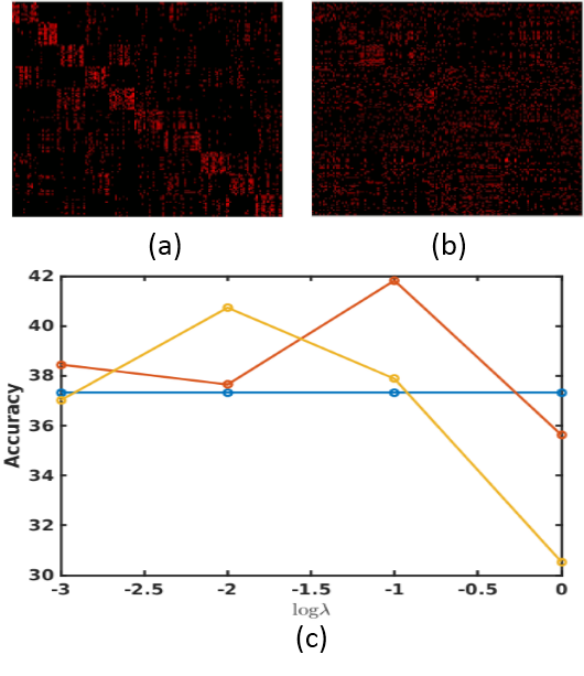
Fig. 3: Matching Matrix $\mathbf{C}$. (a) With $\lambda_{g}=0.01$. (b) With $\lambda_{g}=0$. (c) Accuracy values for different $\lambda_{2},\lambda_{3}$. This is for $A\rightarrow W$ task.

We compared our approach against popular non-deep domain adaptation methods. Current methods involve deep architectures and would not compare fairly. So we include (a) The no adaptation baseline (NA), which consists of using the original classifier without adaptation; (b) Geodesic Flow Kernel (GFK) [8]; (c) Subspace Alignment (SA) [10]; (d) Joint Distribution Adaptation (JDA) [24], which jointly adapts both marginal and conditional distributions along with dimensionality reduction; (e) Correlation Alignment (CORAL) [11] and (f) Optimal Transport (OT) [13].

The comparison results are shown in Table 1. We see that in almost all the cases, local DA methods like OT and our proposed method dominated over other global methods. Moreover, our method dominates over OT for most of the tasks. This is because our method exploits higher order structural similarity between the source and target data points. Also, in situations where OT is slightly better than our methods, the source and target data do not have enough structurally similar regions.

We also performed experiments to see how initial clustering affects recognition performance of our proposed method. We see the results in Table 1 for $\eta=0.75,0.5$; that is, when the number of exemplars are around $75\%,50\%$ of the total number of data-points, respectively. In general, the results showed decrease in performance with respect to $\eta=1$ but are still competitive with respect to some of the previous methods. The only exception is in the tasks $C\rightarrow W$, $A\rightarrow C$ and $W\rightarrow A$, where for decreasing $\eta$, the accuracy increases. This is because decreasing the number of exemplars decreases the possibility of including outliers as unwanted nodes in constructing the graph. Moreover, we analyzed the effect of regularization parameters $\lambda_{2},\lambda_{3},\lambda_{g}$ on the $A\rightarrow W$ task. Fig. 3 (a) and (b) showed the matching matrix ${\bf C}$ for $\lambda_{g}=0.01$ and $\lambda_{g}=0$, respectively. The rows and columns in the matrix ${\bf C}$ represent the source and target, respectively. In Fig. 3(a), for $\lambda_{g}=0.01$, we see that 10 block-diagonal matrices representing all the 10 common categories appear as heatmap on the matrix ${\bf C}$. It suggests that the group lasso regularizer allows discrimination of the classes more accurately compared to Fig. 3(b) that is with $\lambda_{g}=0$, where we have matching matrix ${\bf C}$ with more uniform entries.

In Fig. 3 (c), we show the effect of varying $\lambda_{2}$ and $\lambda_{3}$. The blue straight line shows the accuracy result when $\lambda_{2}=\lambda_{3}=0$. The yellow line shows the accuracy result when $\lambda_{2}=0$ and $\log_{10}\lambda_{3}$ is varied. The red line shows the accuracy result when $\lambda_{3}=0$ and $\log_{10}\lambda_{2}$ is varied. The results suggest that including the higher order cost terms without weighing them heavily in the cost function improves performance over solely using the first-order matching.

4 CONCLUSION

This paper proposed the use of hyper-graph matching between the source and target domains, which have previously not been used for unsupervised domain adaptation. We also proposed a computationally efficient optimization routine based on conditional gradient and ADMM. Results on object recognition dataset suggested our proposed UDA method to be competitive with respect to previous methods. In the future, we plan to extend our method to deep architectures that will learn the representations as well.

References

- [1] Antonio Torralba and Alexei A Efros, “Unbiased look at dataset bias,” in IEEE CVPR, 2011, pp. 1521–1528.
- [2] Bianca Zadrozny, “Learning and evaluating classifiers under sample selection bias,” in ICML, 2004, p. 114.
- [3] Takafumi Kanamori, Shohei Hido, and Masashi Sugiyama, “Efficient direct density ratio estimation for non-stationarity adaptation and outlier detection,” in NIPS, 2009, pp. 809–816.
- [4] Masashi Sugiyama, Shinichi Nakajima, Hisashi Kashima, Paul V Buenau, and Motoaki Kawanabe, “Direct importance estimation with model selection and its application to covariate shift adaptation,” in NIPS, 2008, pp. 1433–1440.
- [5] Jiayuan Huang, Alexander J Smola, Arthur Gretton, Karsten M Borgwardt, and Bernhard Schölkopf, “Correcting sample selection bias by unlabeled data,” in NIPS, 2007, p. 601.
- [6] Raghuraman Gopalan, Ruonan Li, and Rama Chellappa, “Unsupervised adaptation across domain shifts by generating intermediate data representations,” IEEE TPAMI, vol. 36, no. 11, pp. 2288–2302, 2014.
- [7] Raghuraman Gopalan, Ruonan Li, and Rama Chellappa, “Domain adaptation for object recognition: An unsupervised approach,” in IEEE ICCV, 2011, pp. 999–1006.
- [8] Boqing Gong, Yuan Shi, Fei Sha, and Kristen Grauman, “Geodesic flow kernel for unsupervised domain adaptation,” in IEEE CVPR, 2012, pp. 2066–2073.
- [9] Boqing Gong, Kristen Grauman, and Fei Sha, “Connecting the dots with landmarks: Discriminatively learning domain-invariant features for unsupervised domain adaptation.,” in ICML, 2013, pp. 222–230.
- [10] Basura Fernando, Amaury Habrard, Marc Sebban, and Tinne Tuytelaars, “Unsupervised visual domain adaptation using subspace alignment,” in IEEE ICCV, 2013, pp. 2960–2967.
- [11] Baochen Sun, Jiashi Feng, and Kate Saenko, “Return of frustratingly easy domain adaptation,” in AAAI, 2016.
- [12] Sinno Jialin Pan, Ivor W Tsang, James T Kwok, and Qiang Yang, “Domain adaptation via transfer component analysis,” IEEE Trans. Neural Networks, vol. 22, no. 2, pp. 199–210, 2011.
- [13] Nicolas Courty, Rémi Flamary, Devis Tuia, and Alain Rakotomamonjy, “Optimal transport for domain adaptation,” IEEE TPAMI, vol. 39, no. 9, pp. 1853–1865, 2017.
- [14] Olivier Duchenne, Francis Bach, In-So Kweon, and Jean Ponce, “A tensor-based algorithm for high-order graph matching,” IEEE TPAMI, vol. 33, no. 12, pp. 2383–2395, 2011.
- [15] D Khuê Lê-Huu and Nikos Paragios, “Alternating direction graph matching,” in IEEE CVPR, 2017, pp. 6253–6261.
- [16] Delbert Dueck and Brendan J Frey, “Non-metric affinity propagation for unsupervised image categorization,” in IEEE ICCV, 2007, pp. 1–8.
- [17] Jerome Friedman, Trevor Hastie, and Robert Tibshirani, “A note on the group lasso and a sparse group lasso,” arXiv preprint arXiv:1001.0736, 2010.
- [18] Marguerite Frank and Philip Wolfe, “An algorithm for quadratic programming,” Naval Research Logistics (NRL), vol. 3, no. 1-2, pp. 95–110, 1956.
- [19] Martin Jaggi, “Revisiting frank-wolfe: Projection-free sparse convex optimization.,” in ICML, 2013, pp. 427–435.
- [20] Stephen Boyd et al., “Distributed optimization and statistical learning via the alternating direction method of multipliers,” Foundations and Trends® in Machine Learning, vol. 3, no. 1, pp. 1–122, 2011.
- [21] Kate Saenko, Brian Kulis, Mario Fritz, and Trevor Darrell, “Adapting visual category models to new domains,” in ECCV, 2010, pp. 213–226.
- [22] G. Griffin, A. Holub, and P. Perona, “Caltech-256 object category dataset,” Tech. Rep. 7694, California Institute of Technology, 2007.
- [23] Herbert Bay, Tinne Tuytelaars, and Luc Van Gool, “Surf: Speeded up robust features,” in ECCV, 2006, pp. 404–417.
- [24] Mingsheng Long, Jianmin Wang, Guiguang Ding, Jiaguang Sun, and Philip S Yu, “Transfer feature learning with joint distribution adaptation,” in IEEE ICCV, 2013, pp. 2200–2207.