A simple derivation of the two force laws for elliptic orbits from Proposition 6 in Newton’s Principia

Abstract.

Based on Propostion 6 of his Principia, Newton’s geometrical derivation in Propositions 10 and 11 for the radial dependence of the two central forces that lead to elliptical orbits is notoriously difficult. An alternate and more transparent derivation is obtained by applying the affine transformation of a circle into an ellipse.

1. Introduction

In 1684, when Edmond Halley visited Isaac Newton and asked him if the knew the orbital curve for an inverse square force, Newton promptly responded that it is an ellipse. But when asked for his calculation, he could not find it, and when he tried the derivation again he could not reproduce it [1]. But several months later he sent him a short treatise entitled De Motu Corporum Gyratum containing a proof, which appeared in his Principia as Proposition 11. His proof, based on a general expression for central forces in Proposition 6, is notoriously difficult to understand. For example, in the“Guide to Newton Principia”, I. B. Cohen devoted six pages to describe it [2], while in the “The Key to Newton’s Dynamics”, Bruce Brackenridge took eleven pages for the same task [3]. Even Richard Feynman complained that he couldn’t follow Newton’s proof [4], and developed an alternate one that turned out to have been given previously by J. C Maxwell [5] who in turn attributed it to Sir William Hamilton. At the start of $18th$ century, however, able mathematicians like Jacob Hermann, Pierre Varignon and Johann Bernoulli were able to express Newton’s relation for central force in Proposition 6 as a differential equation for the orbit in Cartesian coordinates, while Gotfried Leibniz obtained such an equation in polar coordinates [6].

Given a continuous curve and a fixed point, in Proposition 6 Newton gave an expression in geometrical form for the attractive central force $f$ acting on a body that is confined to move along this curve, describing areas proportional to the time elapsed according to Proposition 1, and in Propositions 10 and 11 he treated the cases when this curve is an ellipse. In Proposition 10 the center of force is placed at the center of the ellipse, and he proved that the resulting force depends linearly on the distance from this center, while in Proposition 11 he treated the case relevant to planetary motion when the center of force is at a focus of the ellipse, and proved that the force varies inversely with the square of the distance from the center.

Referring to the diagram for Proposition 6 reproduced in Fig.1, Newton’s relation for a central force is

(1) $$f\propto\frac{QR}{SP^{2}\times QT^{2}},$$

where SP is the radial distance of a body at P, revolving around the center of force at S on the orbital curve APQ, Q is near P, and QT is a line perpendicular to SP. The location of R appears to be at the intersection of the line ZPY tangent to the curve at P with the extension of the radial line SQ, and then QR=SR-SQ. The product $SP\times QT$ is the area of the triangle SPQ, which is proportional to the time interval for the motion of a body from P to Q, according to Proposition 1. When the curve APQ is expressed in polar coordinates ($r,\theta$), it is straightforward to calculate this differential area:

(2) $$SP\times QT=r(\theta)^{2}\delta\theta.$$

where $\delta\theta$ is the first order differential angle between the radial lines $SP=r(\theta)$ and $SQ=r(\theta+\delta\theta)$, (see Fig. 2). The difficult problem is to evaluate QR which must be a second order differential for the central force $f$, Eq.1, to exist in the continuum limit when $\delta\theta\rightarrow 0$. In the first edition of the Principia (1687), Proposition 6 states: “QR should be drawn parallel to the distance SP” [3], as shown also in the diagrams associated with Propositions 10 and 11. But the diagram in Fig.1 associated with Proposition 6, shows QR drawn parallel to SQ. This difference does not have any practical consequence, because QP is a first order differential that becomes arbitrarily small in the continuum limit, but it matters for the method adopted to evaluate the magnitude of QR. In Propositions 10 and 11, Newton took QR parallel to SP.

In Section 2 the affine transformation that relates the ellipse to a circle is applied to obtain the displacement QR , and the radial dependence of the force f, Eq. 1, is obtained when the center of force is located at a focus of the ellipse corresponding to Proposition 11. In Section 3 the case corresponding to Proposition 10 is treated when the center of force is at the center of the ellipse, corresponding to Proposition 10. An Appendix contains a brief historical account of Robert Hooke’s remarkable graphic and analytic treatment of this problem in 1685.

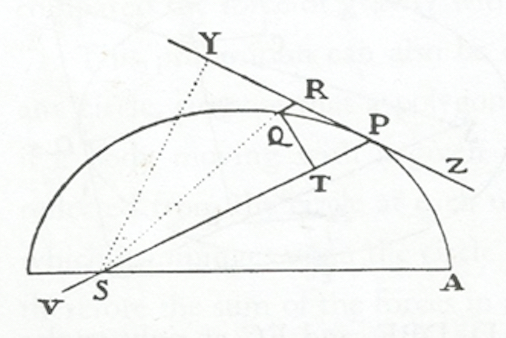
Figure 1. Diagram for Proposition 6

2. Proposition 11, Inverse Square force

Referring to Fig.2, $x_{P}^{\prime}$, $y_{P}^{\prime}$ are the Cartesian coordinates of a point P’ on the circle of radius $a=CA$ centered at C, and $x_{P}=x_{P}^{\prime}-a\epsilon$ and $y_{P}=\lambda y_{P}^{\prime}$ are the corresponding coordinates of a point P on the ellipse obtained by the affine transformation with parameter $\lambda$. The ellipse coordinates are given relative to the focus of the ellipse at S, where $CS=a\epsilon$, $\lambda=\sqrt{1-\epsilon^{2}}$, and $\epsilon$ is the eccentricity of the ellipse. Then

(3) $$tan\theta=\frac{y_{P}}{x_{P}}=\frac{\lambda sin\theta^{\prime}}{(cos\theta^{\prime}-\epsilon)}$$

gives the relation between the angles $\theta$ and $\theta^{\prime}$ for the radial lines r=SP and r’=CP’ relative to CA. We have $r=a(1-\epsilon cos\theta^{\prime})$, and substituting $cos\theta^{\prime}=(cos\theta+\epsilon)/(1+\epsilon cos\theta)$ one obtains

(4) $$r=\frac{a(1-\epsilon^{2})}{1+\epsilon cos\theta},$$

the well known equation for the ellipse in polar coordinates.

The first order differential angle $\delta\theta$ between the nearby radial lines SP and SQ, and $\delta\theta^{\prime}$ between the lines CP’ and CQ’ are related by

(5) $$\frac{\delta\theta}{\cos^{2}\theta}=\frac{\lambda\delta\theta^{\prime}(1-\epsilon cos\theta^{\prime})}{(cos\theta^{\prime}-\epsilon)^{2})}.$$

Substituting $cos\theta^{\prime}=(r/a)cos\theta+\epsilon$, and $r/a=(1-\epsilon^{2})/(1+\epsilon cos\theta$) for the equation of the ellipse in polar coordinates, Eq. 4, one finds

(6) $$\delta\theta=\frac{\lambda a}{r}\delta\theta^{\prime}$$

Newton’s measure for the central force f in Proposition 6 is

(7) $$f\propto\frac{QR}{QT^{2}\times SP^{2}},$$

where $QT\times SP=r^{2}\delta\theta$ is the differential area, and according to Eq.6

(8) $$r^{2}\delta\theta=rb\delta\theta^{\prime},$$

where $b=\lambda a$ is the minor axis of the ellipse.

The point R is located at the intersection of the tangent line at P and the extension of the radial line CQ; hence QR=SR-SQ (see Fig.1). Since a tangent line on the circle is orthogonal to the radial line, it is straightforward to locate the intersection R’ of the tangent line at P’ with the extension of the line CQ’, and we have

(9) $$CR^{\prime}=\sqrt{a^{2}+(a\delta\theta^{\prime})^{2}}=a(1+\frac{\delta\theta^{\prime 2}}{2})$$

to second order in $\delta\theta^{\prime}$. Hence

(10) $$Q^{\prime}R^{\prime}=CR^{\prime}-CQ^{\prime}=\frac{1}{2}a\delta\theta^{\prime 2},$$

and by the affine transformation

(11) $$QR=\frac{1}{2}a\delta\theta^{\prime 2}\sqrt{cos^{2}\theta^{\prime}+\lambda^{2}sin^{2}\theta^{\prime}},$$

where

(12) $$cos\theta^{\prime}=\frac{(\epsilon+cos\theta)}{(1+\epsilon cos\theta)},$$

according to Eq. 3. Substituting this relation between the cosines of the angles $\theta$ and $\theta^{\prime}$ in Eq.11, one finds that

(13) $$QR=Q^{\prime}R^{\prime}=\frac{1}{2}a\delta\theta^{\prime 2}$$

The diagram in Fig.2 shows that QR does not lay along the extension of SR and differs in magnitude from Q’R’, but this relation is valid because $\delta\theta$ and $\delta\theta^{\prime}$ are first order differentials. Hence, applying Newton’s expression for force, Eq. 7, and for the differential area, Eq. 8 , we obtain

(14) $$f=\frac{QR}{SP^{2}\times QT^{2}}=\frac{a}{2r^{2}b^{2}}=\frac{1}{SP^{2}\times L},$$

in accordance with Proposition 11, where $L=2BC^{2}/AC$ is the latus rectum of the ellipse.

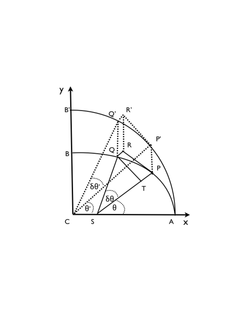
Figure 2. AP’Q’B’ is a quarter of a circle with center at C and radius CA, APQB is the corresponding section of an ellipse obtained from the affine transformation x=x’, y=$\lambda y$, where $\lambda=\sqrt{1-\epsilon^{2}}$, and S is a focus of the ellipse where CS=$\epsilon CA$.

3. Proposition 10, Linear force

Referring to Fig.3, $x_{P}^{\prime}=acos\theta^{\prime}$, $y_{P}^{\prime}=asin\theta^{\prime}$ are the Cartesian coordinates of P’ on the circle of radius $a$, and by the affine transformation, $x_{P}=x_{P}^{\prime},y_{P}=\lambda y_{P}^{\prime}$ are the corresponding coordinates of P on the ellipse with major axis $a=CA$, and minor axis $b=\lambda a=BC$. Then

(15) $$\frac{y_{P}}{x_{P}}=tan\theta=\lambda tan\theta^{\prime},$$

and

(16) $$\frac{\delta\theta}{\cos^{2}\theta}=\frac{\lambda\delta\theta^{\prime}}{cos^{2}\theta^{\prime}}$$

The radial distance $r=PC$ is

(17) $$r=a\sqrt{cos^{2}\theta^{\prime}+\lambda^{2}sin^{2}\theta^{\prime}}=\frac{a}{\sqrt{cos^{2}\theta+sin^{2}\theta/\lambda^{2}}}$$

and

(18) $$QR=Q^{\prime}R^{\prime}\sqrt{cos^{2}\theta^{\prime}+\lambda^{2}sin^{2}\theta^{\prime}},$$

where according to Eq.11 $Q^{\prime}R^{\prime}=a\delta\theta^{\prime 2}/2$. Therefore

(19) $$QR=\frac{\lambda r\delta\theta^{\prime 2}}{2}.$$

and the differential area

(20) $$QT\times PC=r^{2}\delta\theta=a^{2}\lambda\delta\theta^{\prime}.$$

Hence, the central force

(21) $$f=\frac{QR}{QT^{2}\times PC^{2}}=\frac{r}{2b^{2}a^{2}}=\frac{PC}{2BC^{2}AC^{2}}$$

in accordance with Newton’s result in Proposition 10.

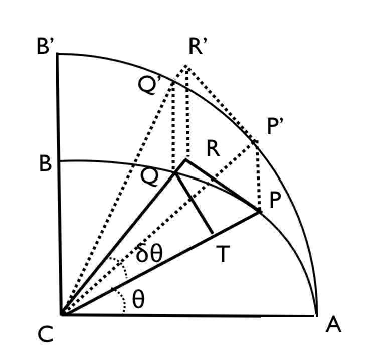
Figure 3. AP’Q’B’ is a quarter of a circle with center at C and radius CA, APQB is the corresponding section of an ellipse obtained from the affine transformation x=x’, y=$\lambda y$

Appendix

In 1685, when Newton sent the first draft of his Principia entitled De Motu Corporum Gyrum to the Royal Society, Robert Hooke who was its secretary at the time, recognized that Newton’s geometrical construction in Theorem 1 could be applied as a graphical method to calculate orbits[7], [8]. He then proceeded to draw such an orbit for a periodic sequence of impacts that depended linearly on the distance from the center of force, and obtained a discrete polygon with the vertices located on an ellipse[9]. Six years earlier, he had communicated to Newton his own ideas about the nature of gravitational forces that accounted for planetary motion along the lines that Newton afterwards implemented. Part of Hooke’s proof that the vertices of the discrete orbit the had obtained were located on an ellipse was based on the affine transformation of a circle into an ellipse (see Figs. 2 and 3 in reference [7]). But his proof differs from Newton’s proof in Proposition 10 which assumes first the orbital curve to be an ellipse, and then determines the radial dependence of the force that gives rise to such an orbit when the center of force is located at the center of the ellipse. Hooke concluded the discussion associated with his diagram with the remark that “ the polygone becomes various according to the differing degrees of Gravity at Different distances from the center”. It is therefore likely that he would have attempted to obtain graphically also the orbit for an inverse square force - the case of interest for gravitation. But there isn’t any evidence among the manuscripts of Hooke that have been preserved that he carried out this calculation. If he had tried to carry out this calculation graphically with similar initial conditions, he would have found that only the resulting vertices of the discrete orbit for the first seven impacts are located on an ellipse . Afterwards, I have shown that the graph for this orbit diverges which would have presented a puzzle for Hooke [10]. Perhaps for this reason he did not publish his remarkable graphic results.

References

- [1] R.S. Westfall, “Never at Rest, A biography of Isaac Newton”, (Cambridge University Press, 1980) p. 403.
- [2] I. B. Cohen, “Introduction to Newton’s Principia” (Cambridge University Press, Cambridge, 1971) pp. 324-329.
- [3] J.B. Brackenridge, “The Key to Newton’s Dyanmics, The Kepler Problem and the Principia” (University of California Press, Berkeley, 1995) pp. 106-117
- [4] D.L. Goodstein and J.R. Goodstein, “ Feynman’s Lost Lecture, The motion of planets around the Sun” (W.W. Norton & Company, New York, 1996). Feynman remarked that he “ couldn’t follow Newton’s demonstration because “ it involved so many properties of conic sections” pg. 156.
- [5] J. C Maxwell, “Matter and motion” (1877) Reprinted with notes and appendices by Sir Joseph Larmor, London: Society for promoting Christian Knowledge, 1920.
- [6] M. Nauenberg, “ The early application of the calculus to the inverse square force problem”, Archive for History of Exact Science 64 (2010) 297-312
- [7] M. Nauenberg, “Hooke, Orbital Motion and Newton’s Principia”, American Journal of Physics 62 (1994) 331-350
- [8] M. Nauenberg, “Hooke’s and Newton’s Contributions to the Early Development of Orbital Dynamics and the Theory of Universal Gravitation”, Early Science and Medicine, 10 (2005) 518-528.
- [9] Among Hooke’s papers in the Trinity Library, Cambridge, there is a manuscript dated Sept. 1685 that contains Hooke’s drawing of a discrete polygonal orbit with vertices on an ellipse, reproduced in Ref. [7].
- [10] See Figs 5 and 6 in reference [7], pg. 344.