The Ridge Effect, Azimuthal Correlations, and other Novel Features of Gluonic String Collisions in High Energy Photon-Mediated Reactions

Abstract

One of the remarkable features of high-multiplicity hadronic events in proton-proton collisions at the LHC is the fact that the produced particles appear as two “ridges”, opposite in azimuthal angle $\phi$, with approximately flat rapidity distributions. This phenomena can be identified with the inelastic collision of gluonic flux tubes associated with the QCD interactions responsible for quark confinement in hadrons. In this paper we analyze the ridge phenomena when the collision involves a flux tube connecting the quark and antiquark of a high energy real or virtual photon. We discuss gluonic tube string collisions in the context of two examples: electron-proton scattering at a future electron-ion collider or the peripheral scattering of protons accessible at the LHC. A striking prediction of our analysis is that the azimuthal angle of the produced ridges will be correlated with the scattering plane of the electron or proton producing the virtual photon. In the case of $ep\to eX$, the final state $X$ is expected to exhibit maximal multiplicity when the elliptic flow in $X$ is aligned with the electron scattering plane. In the $pp\to ppX$ example, the multiplicity and elliptic flow in $X$ are estimated to exhibit correlated oscillations as functions of the azimuthal angle $\Phi$ between the proton scattering planes. In the minimum-bias event samples, the amplitude of oscillations is expected to be on the order of 2% to 4% of the mean values. In the events with highest multiplicity, the oscillations can be three times larger than in the minimum-bias event samples.

I Introduction

Scattering has been critical to understanding of submicroscopic structure since the earliest stages. Alpha-particle scattering revealed the atomic nucleus, and its components – protons and neutrons. Later, elastic electron scattering found the electric charge distribution of nuclei, and inelastic electron scattering found point-like structure inside the nucleon, while electron-positron pair annihilation revealed also the presence of gluons inside hadrons. The existence of such objects does not necessarily tell the whole story about hadron structure: the arrangement of quark and gluon configurations could be more than just ‘floating’ particles. One possible configuration is a string of gluons connecting quark and anti-quark in a meson, or quark and di-quark in a nucleon. Strings provide a linear structure, so that if two strings are aligned parallel to each other in the plane perpendicular to the collision direction, then their collision can give rise to higher multiplicity than if the strings are oriented transversely to each other. The flow of collision products is also different. It is hence encouraging for thinking about gluon strings that patterns of varying multiplicity and collective flow of products are seen in occasional $pp$ collisions.

I.1 Strings in $ep\to eX$ and $pp\to ppX$ scattering

We suggest that scattering of charged particles may be directly sensitive to the formation of gluon strings Photon2017 . An electron can emit a virtual photon that in turn develops a quark-anti-quark pair connected by a gluon string (see Fig. 1).

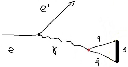
Figure 1: Scattering of an electron yields a virtual photon that develops quark-anti-quark pair connected by a gluon string.

The string azimuthal orientation, defined by the angle $\Phi$ illustrated in Fig. 2, is correlated with the scattering plane of the parent charged particle.

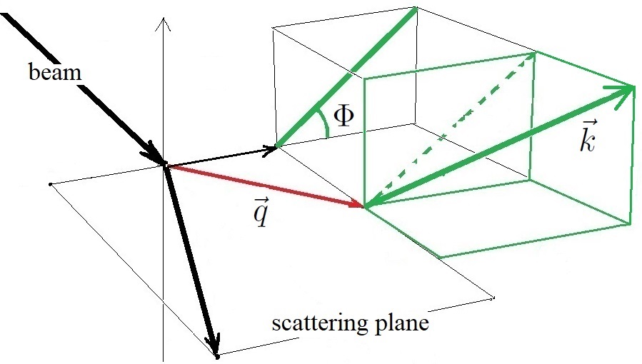
Figure 2: Beam of charged particles is scattered with momentum transfer $\vec{q}$ that defines a scattering plane. The photon that carries $\vec{q}$, creates a quark-anti-quark pair with relative momentum $\vec{k}$. The gluon string lies along that momentum and it forms the azimuthal angle $\Phi$ with the scattering plane.

An example of the probability distribution of string orientation with respect to the scattering plane is shown in Fig. 3. Details of its calculation are described in Sec. III.4.

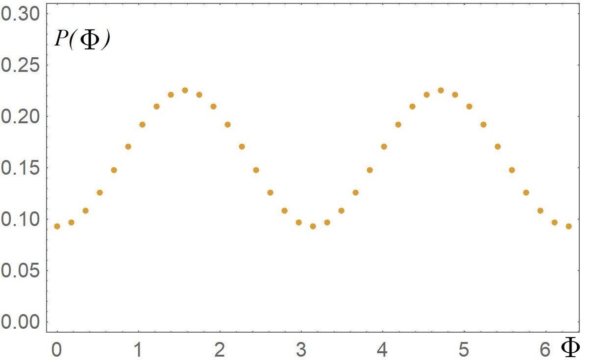
Figure 3: Example of probability $P(\Phi)$ of finding a gluon string produced electromagnetically through scattering of an electron, as a function of the azimuthal angle $\Phi$ around the electron beam between the electron scattering plane and the string axis that connects quark with anti-quark in the string rest frame, see Fig. 2. In the example, the incoming electron momentum is 7 TeV. Electrons scatter elastically with momentum transfers of square $q^{2}=-1.4$ GeV², gaining 1 GeV of momentum transverse to the beam and losing 1/4 of their initial momentum along the beam. Only the strings due to $u\bar{u}$ are accounted for. Inclusion of $d$ and $s$ quark pairs reduces the probability variation amplitude by about one percent. Inclusion of heavy quarks further reduces the variation by about one fifth of the shown magnitude, mostly due to the $c$ quarks that cause about 98% of the latter reduction. The probability plot practically does not change when the electron beam is replaced by a proton beam.

Such a probability distribution implies that the charged-particle scattering-plane azimuthal orientation is correlated with the multiplicity or collective flow of particles that emerge from a subsequent collision of the virtual string with another one that comes from the opposite-going charged particle in the scattering process.

To be specific, when an electron scatters off a proton, through a collision of a string of gluons in a photon with a string that connects a quark and a di-quark in the proton, see Fig. 4,

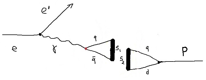
Figure 4: Electron scattering on protons proceeds through a collision of gluon strings, $S_{1}$ that connects a quark and anti-quark in a photon and $S_{2}$ that connects a quark and a di-quark in a proton.

the multiplicity of the final state is optimized when its collective flow is aligned with the electron scattering plane. Similarly, the probability of rare events with large multiplicity and elliptic flow in peripheral $pp$ scattering illustrated in Fig. 5, cf. Bjorken:2013boa ; Lithuania ; Venugopalan1 ; Venugopalan2 , is maximal when one projectile recoil is parallel to the recoil of the opposite-going projectile. For example, such rare

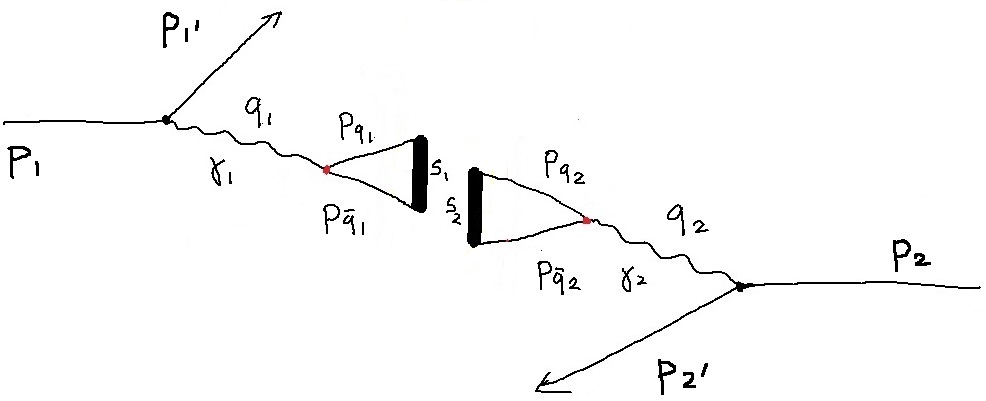
Figure 5: The peripheral $p_{1}p_{2}\to p_{1^{\prime}}p_{2^{\prime}}X$ scattering proceeds through collision of gluon strings $S_{1}$ and $S_{2}$.

large-multiplicity peripheral events with sizable elliptic flow at LHC are expected to have maximal probability of occurring when the two proton scattering planes are parallel to each other. The probability is minimal when the scattering planes of the protons appear rotated by 90 degrees with respect to each other. Figure 6

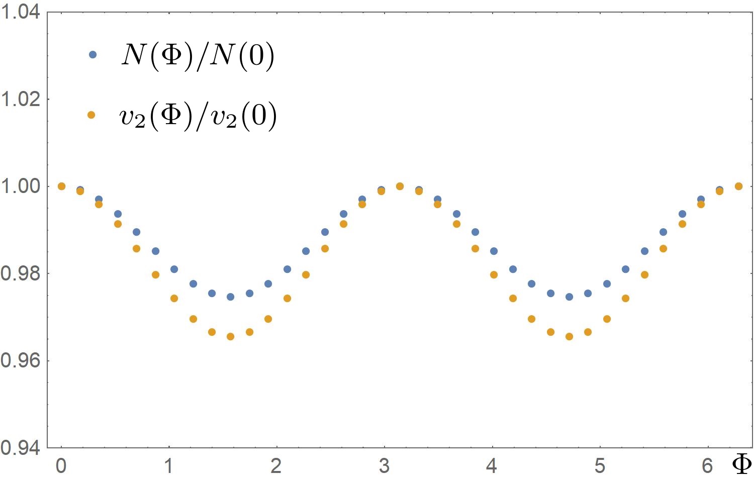
Figure 6: Example of an estimate for the minimal-bias average ratios of multiplicity, $N(\Phi)/N(0)$, and elliptic flow, $v_{2}(\Phi)/v_{2}(0)$, in the $pp$ peripheral scattering process $p_{1}p_{2}\to p^{\prime}_{1}p^{\prime}_{2}X$ at LHC that proceeds through collisions of gluon strings. The ratios are calculated using Eqs. (7) and (8). They depend on the angle $\Phi$ between the two projectile planes that are shown in Fig. 7. Protons come from opposite directions, with momenta equal in size, 7 TeV. They scatter elastically with momentum transfers squared $q_{1}^{2}=q_{2}^{2}=-1.4$ GeV². For example, proton $p_{1}$ scatters horizontally, gaining 1 GeV of momentum transverse to the beam and losing 1/4 of its initial momentum along the beam. Proton $p_{2}$ scatters in a plane forming angle $\Phi$ with the horizontal plane and gains 1 GeV of momentum in that plane transversely to the beam and also loses 1/4 of its initial momentum in the beam direction. The multiplicity is estimated assuming it is proportional to the number of partonic collisions and the elliptic flow is estimated assuming it is proportional to the eccentricity in the initial stage of the string collision. The unknown proportionality constants cancel out in the shown ratios.

illustrates our estimate for string collision effects in terms of the multiplicity $N(\Phi)/N(0)$ and elliptic flow $v_{2}(\Phi)/v_{2}(0)$ in the final state $X$ as functions of the angle $\Phi$ between the planes $(p_{1},p^{\prime}_{1})$ and $(p_{2},p^{\prime}_{2})$ defined by the direction of proton beams and final proton three-momenta $\vec{p}\,^{\prime}_{1}$ and $\vec{p}\,^{\prime}_{2}$ in the laboratory, see Fig. 7.

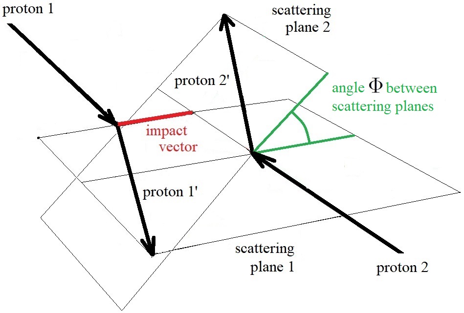
Figure 7: Angle $\Phi$ between scattering planes in Fig. 6.

Figure 6 is obtained using Eqs. (7) and (8). Examples like this suggest that the azimuthal variation of multiplicity and elliptic flow can be used to study properties of gluonic strings in LHC.

Our calculations are carried out using Hamiltonian dynamics in quantum field theory in the approximation of very large beam momentum, and collisions of strings are estimated using a geometrical picture. The strings seen along the proton beam form certain shapes (see Fig. 8)

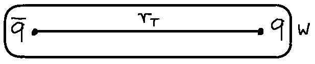
Figure 8: Qualitative view of the two-dimensional string shape in the transverse plane (TP). The length $r_{T}$ corresponds to the vector $\vec{r}_{T}$ that describes the relative position of the quark with respect to the anti-quark, projected on the TP. $w$ denotes the string width. The shape is assigned some thickness distribution, $\rho(\vec{x}_{T})$, that corresponds to the density of partons as function of position $\vec{x}_{T}$ in the TP. The shape of string ends does not matter much if the string length is much bigger than width. In this work, the ends are rectangular, which is the simplest shape to use in our estimates.

in the plane transverse to the beam. Below, this plane is called the transverse plane (TP). The string shape in the TP corresponds to a string that is stretched in space along the vector $\vec{r}$, which extends from the anti-quark to quark in the string rest frame (SRF). When the string moves very fast along the proton beam, its shape in the TP is seen in the laboratory as built around a two-dimensional vector $\vec{r}_{T}$ that forms the transverse part of $\vec{r}=(r_{x},\vec{r}_{T})$. The component $r_{x}$ corresponds to the beam direction in the frame of reference that we work with; its $x$-axis is chosen along the beam. The collision of strings $S_{1}$ and $S_{2}$ proceeds via interaction of partons in the region of overlap of the string shapes on the TP, illustrated in Fig. 9.

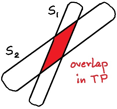
Figure 9: The number of partonic collisions in a collision of two strings $S_{1}$ and $S_{2}$, is assumed to be proportional to the overlap area in the TP, in which the strings are seen as they appear when looked at along the beam.

The magnitude of overlap grows when the angle between the strings decreases, provided that their impact parameter is smaller than the string width. There is a competing effect that the impact parameters may reach values comparable with the string length, much larger than the string width, when the angle between the strings is not small. Therefore, in the minimal bias (MB) averages over events with all possible impact parameters, these effects cancel each other. The resulting azimuthal correlations between projectile planes and the average multiplicity and elliptic flow, are small. They can be enhanced by averaging over events with relatively large multiplicities, discussed later.

Concerning the length and width of gluonic strings, we assume that the typical time needed by a string to reach its full width is longer than the time of stretching a string by quarks. This is in agreement with the flux-tube knot model assumption StringKnots1 ; StringKnots2 that the relaxation of a topologically non-trivial string configuration to a tight-knot state configuration is faster than the configuration decay rate, cf. JohnsonThorn ; IsgurPaton . In the same spirit, we assume that the suddenly stretched string has a diameter as small as $\sim 0.1$ fm. Knowing that hadrons extend over distances order 1 fm, one could consider string models with width related to length, such as $w=r/10$ etc.

One might hope to estimate the shape of gluonic strings in photons using the vector dominance model (VDM) of photon-nucleon coupling. Three issues arise. One is that the VDM does not provide any information on the shapes of flux tubes in virtual $\rho$ mesons. The other issue is that a collision of two photons may proceed through quark-anti-quark pairs whose relative motion is not at all limited as the relative motion of quarks is limited by the wave function of quarks in the neutral $\rho$-meson. The quark-gluon picture is dual to the sum over the whole spectrum of hadronic states that contribute. The third issue is that although the VDM suggests that a photon can interact with an extended proton via a pair of quarks resembling a $\rho$-meson, it does not tell us how a photon can turn into a pair of quarks that do not interact and do not need to overlap with a nucleon’s structure. Having no firm theoretical input concerning the relation between strings’ width $w$ and the distance between quark and anti-quark in a pair in a photon, $r=|\vec{r}\,|$, we consider $w$ a free parameter. Figure 6 is obtained assuming that $w=0.1$ fm.

The magnitude of string overlap is used as a measure of the number of partonic collisions that are possible in a given configuration of strings heading towards each other. Multiplicity is assumed proportional to this number. The shape of the overlap area is used to estimate the eccentricity of the colliding parton-matter in the transverse plane. The eccentricity is used to estimate the elliptic flow in $X$, the latter assumed proportional to the former. The unknown proportionality constants cancel out in ratios shown in Fig. 6.

In an event that leads from protons $p_{1}$ and $p_{2}$ to $p^{\prime}_{1}$ and $p^{\prime}_{2}$, the density of parton-parton collisions in the TP is described using the formula Glauber ; v2varepsilon2 ; dentPLB ; Blaizot J P (2014).

$$n_{\rm coll}(\vec{x}_{T},\vec{b},\vec{r}_{1},\vec{r}_{2}) = \sigma\,\rho_{1}(\vec{x}_{T}-\vec{b}/2,\vec{r}_{1})\,\rho_{2}(\vec{x}_{T}+\vec{b}/2,\vec{r}_{2}).$$

It says that the probability density for finding pairs of partons capable of colliding at the point $\vec{x}_{T}$ in the TP, is proportional to a product of parton probability densities in the parent strings that are separated by the impact vector $\vec{b}$. The photons come from protons almost along the beam and the string impact parameter is assumed the same as the proton-proton impact parameter. The coefficient $\sigma$ stands for the parton-parton cross-section, presumably on the order of a few to ten mb. The string parton densities are determined by the string orientations, $\vec{r}_{1}$ and $\vec{r}_{2}$, in the respective SRFs. Formulas used for estimates of the parton densities in strings are described in Sec. II.

In addition to the string parton densities, evaluation of observables concerning collisions of strings involves probabilities, denoted below by $P(\vec{r}_{1},p^{\prime}_{1},p_{1})$ and $P(\vec{r}_{2},p^{\prime}_{2},p_{2})$, for the string orientation vectors $\vec{r}_{1}$ and $\vec{r}_{2}$. These probabilities are estimated using QED. They depend on the incoming and outgoing protons’ momenta. Protons’ spins are summed and averaged over because we assume that the beam protons are not polarized and final proton polarizations are not measured. Strings are assumed to not depend on the quark spins. The probabilities we use are described in Sec. III.

I.2 Observables associated with string collisions

Consider the example of $pp$ scattering. The density of collisions in Eq. (I.1) is used to estimate multiplicity and ridge effects as functions of the azimuthal angle $\Phi$ between proton planes. The multiplicity $N(\vec{b},\vec{r}_{1},\vec{r}_{2})$ of $X$ is assumed proportional to the number of partonic collisions,

$$N(\vec{b},\vec{r}_{1},\vec{r}_{2}) = C_{N}\ N_{\rm coll}(\vec{b},\vec{r}_{1},\vec{r}_{2})$$ (2)

$$= C_{N}\ \int d^{2}x_{T}\ n_{\rm coll}(\vec{x}_{T},\vec{b},\vec{r}_{1},\vec{r}_{2})\ .$$ (3)

$C_{N}$ denotes an unknown coefficient that can be estimated by comparison with models of string collisions and data on particle production for selected scattering parameters.

The ridge effect is estimated assuming that the elliptic flow $v_{2}$ in $X$ is proportional to the eccentricity $\varepsilon_{2}(\vec{b},\vec{r}_{1},\vec{r}_{2})$ of the density of partonic collisions, $n_{\rm coll}(\vec{x}_{T},\vec{b},\vec{r}_{1},\vec{r}_{2})$, with a model-dependent coefficient on the order of 0.3 v2varepsilon2 . Definition of eccentricity Blaizot J P (2014) uses the concept of averaging of a quantity $f(\vec{x}_{T})$ with the density,

$$\{f\} = \frac{\int d^{2}x_{T}\ f(\vec{x}_{T})\ n_{\rm coll}(\vec{x}_{T},\vec{b},\vec{r}_{1},\vec{r}_{2})}{\int d^{2}x_{T}\ n_{\rm coll}(\vec{x}_{T},\vec{b},\vec{r}_{1},\vec{r}_{2})}\ ,$$ (4)

where it is understood that $\vec{x}_{T}$ is measured from the geometrical center of the overlap area in the TP so that $\{\vec{x}_{T}\}=0$. One introduces polar coordinates in the TP, angle $\alpha$ and length $x_{T}=|\vec{x}_{T}|$, using $\vec{x}_{T}=(x,y)=x_{T}\ (\cos{\alpha},\sin{\alpha})$. Eccentricity is defined in terms of the averaged values of $x^{2}-y^{2}=x_{T}^{2}\cos 2\alpha$ and $2xy=x_{T}^{2}\sin 2\alpha$. Both are contained in the averaged value of the complex quantity $x_{T}^{2}e^{2i\alpha}$. Eccentricity of a density is defined as the modulus of averaged value of this quantity Blaizot J P (2014)

$$\varepsilon_{2}(\vec{b},\vec{r}_{1},\vec{r}_{2}) = \frac{\sqrt{\{x_{T}^{2}\cos(2\alpha)\}^{2}+\{x_{T}^{2}\sin(2\alpha)\}^{2}}}{\{x_{T}^{2}\}}\ .$$ (5)

The square root of sum of squares of averaged values reflects the relationship between real and imaginary parts of a complex number and its modulus.

The differential string-collision cross section can be estimated using the formula Glauber ; dentPLB ; Goldhaber1 ; Goldhaber2

$${d^{2}\sigma(\vec{b},\vec{r}_{1},\vec{r}_{2}\,)\over db_{y}db_{z}} = 1-e^{-N_{\rm coll}(\vec{b},\vec{r}_{1},\vec{r}_{2})}\ ,$$ (6)

which corresponds to the assumption that the dominant angle dependence comes from strings that are made of similar numbers of gluons, $N_{g}$, large enough to justify the use of an exponential form. Otherwise, a formula $(1-N_{\rm coll}/N_{g}^{2})^{N_{g}^{2}}$ may be used. The examples shown in Fig. 6 are obtained using Eq. (6).

Estimates for the MB-averaged $\Phi$-dependence of multiplicity and elliptic flow, shown in Fig. 6, result from integration over the impact vector $\vec{b}$. We use the formulas

$$N(p^{\prime}_{1},p^{\prime}_{2}) = {C_{N}\over\sigma_{\rm p}}\int d^{2}b$$ (7)

$$\times \int d^{3}r_{1}\ P(\vec{r}_{1},p^{\prime}_{1},p_{1})\int d^{3}r_{2}\ P(\vec{r}_{2},p^{\prime}_{2},p_{2})$$

$$\times \left[1-e^{-N_{\rm coll}(\vec{b},\vec{r}_{1},\vec{r}_{2})}\right]\ N_{\rm coll}(\vec{b},\vec{r}_{1},\vec{r}_{2})\ ,$$

$$v_{2}(p^{\prime}_{1},p^{\prime}_{2}) = {C_{v}\over\sigma_{\rm p}}\int d^{2}b$$ (8)

$$\times \int d^{3}r_{1}\ P(\vec{r}_{1},p^{\prime}_{1},p_{1})\int d^{3}r_{2}\ P(\vec{r}_{2},p^{\prime}_{2},p_{2})$$

$$\times \left[1-e^{-N_{\rm coll}(\vec{b},\vec{r}_{1},\vec{r}_{2})})\right]\ \varepsilon_{2}(\vec{b},\vec{r}_{1},\vec{r}_{2})\ ,$$

where $\sigma_{\rm p}$ is a total cross section normalization factor that cancels out in the ratios of interest in Fig. 6. The normalization factor will not be further discussed. We only mention that its calculation requires integration over all possible final states. Similarly, the unknown proportionality constant $C_{v}$, assumed to relate elliptic flow to eccentricity, cancels out in the ratios of Fig. 6. Consequently, we focus on the eccentricity that is meant to yield directly the ratio shown in Fig. 6 for the elliptic flow.

II Geometrical overlap of strings

Modeling of string collisions involves consideration of rotations and boosts required for description of the off-shell string world-sheets in different frames of reference. However, the fast motion of a quark-di-quark or quark-anti-quark pair along the beam implies a simple picture in the TP. We limit explicit discussion to quark-anti-quark pairs from photons.

II.1 String shape in the transverse plane

In the laboratory, a string specified by the quark-anti-quark relative position vector, $\vec{r}$ in the SRF, moves very fast along the proton beam. The beam is used to define the laboratory $x$-axis. The string has the same width $w$, transverse to the beam, in both frames. The length and orientation of the string on the TP are determined by the vector $\vec{r}_{T}$, which is the transverse part of $\vec{r}$, and a correction due to the string width (see below). The string shape in the TP has some density profile, coming from the string structure and orientation in space. In the TP region where the string density differs from zero, it is useful to set the string thickness to its average value, say, $\bar{\rho}_{1}$ for string $S_{1}$ and $\bar{\rho}_{2}$ for $S_{2}$. This approximation greatly simplifies estimates of angular correlations.

If a string forms an angle $\beta$ with the TP, which is the angle it makes with the $yz$-plane in the SRF, its projection on that plane is described by the vector $\vec{l}$ of length

$$l = (r+w)|\cos{\beta}|+w|\sin{\beta}|\ ,$$ (9)

where $r=|\vec{r}\,|$ and $\sin\beta=r_{x}/r$. The two-dimensional string shape in the TP is assumed to be a rectangle of area $a_{\beta}=wl$. The string average parton probability density on the TP, $\bar{\rho}$, times the area $a_{\beta}$, gives the same number of partons, $N_{g}$, described by the formula $\bar{\rho}a_{\beta}$, as a product of the average three dimensional parton probability density in the string, $\rho$, times the string volume, $\rho(r+w)\pi w^{2}/4$. This implies

$$\bar{\rho} = {\rho\pi w(r+w)/4\over(r+w)|\cos{\beta}|+w|\sin{\beta}|}\ .$$ (10)

In this approximation, the product of parton densities is

$$\rho_{1}(\vec{x}_{T}-\vec{b}/2,\vec{r}_{1})\ \rho_{2}(\vec{x}_{T}+\vec{b}/2,\vec{r}_{2})$$ (11)

$$= \bar{\rho}_{1}\ \bar{\rho}_{2}\ A_{1}(\vec{x}_{T}-\vec{b}/2,\vec{r}_{1})\ A_{2}(\vec{x}_{T}+\vec{b}/2,\vec{r}_{2})\ ,$$

where $A_{1}$ and $A_{2}$ denote the characteristic functions of the two string shapes on the TP. The two strings may a priori have different widths, $w_{1}$ and $w_{2}$. These widths may be correlated with the string lengths, as an element of modeling of how strings develop. The characteristic function of the overlap area is denoted by $A(\vec{x}_{T},\vec{b};\vec{r}_{1},\vec{r}_{2})=A_{1}(\vec{x}_{T}-\vec{b}/2,\vec{r}_{1})\ A_{2}(\vec{x}_{T}+\vec{b}/2,\vec{r}_{2})$. In our estimates, we only consider fixed, small $w_{1}=w_{2}=w=1/10$ fm.

II.2 Thin string approximation

The thin strings approximation means that the string width $w$ is typically much smaller than its length $r$. For thin strings, the dominant overlap shape is a rhombus, as illustrated in Fig. 10.

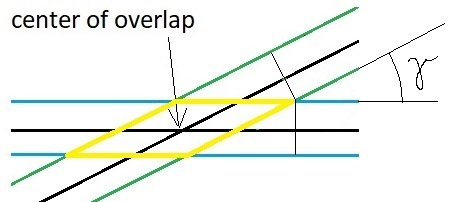
Figure 10: Rhombus overlap area for thin strings.

It is dominant in the sense that a rhombus occurs for most of the impact parameters and for most lengths $l_{1}$ and $l_{2}$ of the strings and most angles $\gamma$ between them. The rhombus area and eccentricity are

$$a_{\rm rhombus} = w^{2}/|\sin\gamma\,|\ ,$$ (12)

$$\varepsilon_{2\,\rm rhombus} = |\cos\gamma\,|\ .$$ (13)

Note that these quantities do not depend on the string lengths. Departures from the rhombus shape occur for small $\gamma$ or when one string overlaps the other with its end.

III Probability of a string

We consider $pp$ scattering. Equations (7) and (8) provide expectation values of multiplicity $N(\vec{b},\vec{r}_{1},\vec{r}_{2})$ and eccentricity $\epsilon(\vec{b},\vec{r}_{1},\vec{r}_{2})$, averaged over string lengths and orientations described in terms of vectors $\vec{r}_{1}$ and $\vec{r}_{2}$. The probability densities, $P(\vec{r}_{1},p^{\prime}_{1},p_{1})$ and $P(\vec{r}_{2},p^{\prime}_{2},p_{2})$, are estimated using the canonical QED Hamiltonian in the instant form (IF) of dynamics Dirac1 in the Coulomb, or radiation gauge BD , in which protons are treated as extended particles with form factors, and quarks are coupled to photons as point-like particles. Formulas for electrons are obtained by removing the form factors. The limit of large projectile energy allows us also to use the infinite momentum frame approximation, which leads to the advantage of using results of the front form of dynamics and, in particular, light-front holography zeta1 ; zeta2 for estimates of the string probability, in addition to the estimates based on the IF linear potential, e.g., see Sec. III.2.

The quark-anti-quark pair creation term in the Hamiltonian acts off energy shell. Therefore, when the pair current is contracted with the physical proton momentum transfer, one does not obtain zero, even if one assumes, as we do, that the electromagnetic production of off-shell $q\bar{q}$ pairs is fully expressible in terms of the physical momentum transfer $q^{\mu}=p^{\mu}-p^{\prime\mu}$ between the initial proton $p$ and the final one, $p^{\prime}$. In order to remove the off-shell current non-conservation effect, one can replace the canonical pair current off shell by

$$j^{\mu}_{\rm pair} \to j^{\mu}_{\rm cons}\,=\,j^{\mu}_{\rm pair}-{j_{\rm pair}q\ q^{\mu}\over q^{2}}\ .$$ (14)

Since the proton current is conserved, the conserved pair current coupling through $g_{\mu\nu}$ to the proton current, $j_{\rm cons}j_{\rm proton}$ is the same as $j_{\rm pair}j_{\rm proton}$. The same result is obtained using the Feynman gauge.

III.1 String amplitude

The Hamiltonian terms that describe the dynamics of quark pairs with strings, $q\bar{q}S$, and protons, $p$, as eigenstates of the Hamiltonian of QCD, completed with the two lowest-order QED interactions of these particles and photons, $\gamma$, is written as BD

$$H = H_{0}+H_{1}+H_{2}\ .$$ (15)

The subscripts denote powers of electric charge. In the intuitive notation, relevant terms are

$$H_{0} = H_{\gamma}+H_{q\bar{q}S}+H_{p}\ ,$$ (16)

$$H_{1} = H_{q\bar{q}S\,\gamma}+H_{\gamma\,q\bar{q}S}+H_{\gamma p^{\prime}\,p}+H_{p\,\gamma p^{\prime}}\ ,$$ (17)

$$H_{2} = H_{q\bar{q}Sp^{\prime}\,p}+H_{p\,q\bar{q}Sp^{\prime}}+\delta H_{p}\ .$$ (18)

The term $\delta H_{p}$ denotes the proton electromagnetic self-energy counter-term, cf. GellMannGoldberger . The proton eigenstate of $H$ is written as a superposition of just three components, neglecting terms that eventually do not contribute to the string probability at order $e^{4}$,

$$|{\rm proton}\rangle = N_{\rm proton}\left(\ |p\rangle+|\gamma p^{\prime}\rangle+|q\bar{q}S\,p^{\prime}\rangle\ \right)\ .$$ (19)

It is normalized by the constant $N_{\rm proton}$ so that $\langle{\rm proton}|{\rm proton}\rangle=E_{p}V$, where $V$ is the large volume in laboratory frame, in which the quantum theory is developed. Including proton spin, $\langle{\rm proton}\ s|{\rm proton}^{\prime}\ s^{\prime}\rangle=2E_{p}(2\pi)^{3}\delta^{3}(p-p^{\prime})\delta_{ss^{\prime}}$. In the formal scattering theory GellMannGoldberger , the eigenvalue equation,

$$H|{\rm proton}\rangle = E_{p}|{\rm proton}\rangle\ ,$$ (20)

determines the amplitude of string component in the form

$$\langle q\bar{q}S\,p^{\prime}|{\rm proton}\rangle\,=\,{N_{\rm proton}\over E_{p}-E_{p^{\prime}}-E_{q\bar{q}}+i\epsilon}$$ (21)

$$\times \sum_{\gamma}{\langle q\bar{q}S|H_{q\bar{q}S\,\gamma}|\gamma\rangle\ \langle\gamma p^{\prime}|H_{\gamma p^{\prime}\,p}|p\rangle\over E_{p}-E_{p^{\prime}}-E_{\gamma}^{-}+i\epsilon}$$

$$+ {N_{\rm proton}\ \langle q\bar{q}S\,p^{\prime}|H_{q\bar{q}S\,p^{\prime}\,p}|p\rangle\over E_{p}-E_{p^{\prime}}-E_{q\bar{q}}+i\epsilon}\ .$$

The matrix elements on the right-hand side are defined by the assumption that once the quark pair is created in a pointlike event according to QED, the quark and anti-quark move away from each other and stretch the string $S$. Thus, the matrix element $\langle q\bar{q}S|H_{q\bar{q}S\,\gamma}|\gamma\rangle$ is equal to the QED amplitude for the point-like event of creation of the pair, $\langle q\bar{q}S|H_{q\bar{q}S\,\gamma}|\gamma\rangle=\langle q\bar{q}|H_{q\bar{q}\,\gamma}|\gamma\rangle=e_{q}\,\bar{u}_{q}\gamma_{\mu}v_{\bar{q}}\ \epsilon^{\mu}_{\gamma}\ 16\pi^{3}\delta^{3}(p_{q}+p_{\bar{q}}-p_{\gamma})\ \delta_{c_{q}c_{\bar{q}}}$. Similarly, the Coulomb matrix element $\langle q\bar{q}S\,p^{\prime}|H_{q\bar{q}S\,p^{\prime}\,p}|p\rangle$ is equal to the QED amplitude $\langle q\bar{q}\,p^{\prime}|H_{q\bar{q}\,p^{\prime}\,p}|p\rangle$ for the transition $p\to q\bar{q}\ p^{\prime}$. Assuming that the string is stretched independently of the spins, flavors and colors of quarks, we have

$$\langle q\bar{q}S\,p^{\prime}|{\rm proton}\rangle\,=\,{N_{\rm proton}\over E_{p}-E_{p^{\prime}}-E_{q\bar{q}}+i\epsilon}$$ (22)

$$\times \sum_{\gamma}{\langle q\bar{q}|H_{q\bar{q}\,\gamma}|\gamma\rangle\ \langle\gamma p^{\prime}|H_{\gamma p^{\prime}\,p}|p\rangle\over E_{p}-E_{p^{\prime}}-E_{\gamma}^{-}+i\epsilon}$$

$$+ {N_{\rm proton}\ \langle q\bar{q}\,p^{\prime}|H_{q\bar{q}\,p^{\prime}\,p}|p\rangle\over E_{p}-E_{p^{\prime}}-E_{q\bar{q}}+i\epsilon}\ .$$

III.2 String length and orientation

The string is stretched by the quarks along their relative momentum $\vec{k}$ in the SRF. At creation, the quark has momentum $\vec{k}$ and the anti-quark $-\vec{k}$. Their invariant mass is ${\cal M}_{q\bar{q}}=2\sqrt{m_{q}^{2}+\vec{k}^{\,2}}$. The outward quark motion is slowed down by the buildup of a string. In the holography zeta1 ; zeta2 motivated by the AdS/QCD duality idea, the buildup is described by the decrease of ${\cal M}_{q\bar{q}}^{2}$ and increase of the effective potential $U_{\rm eff}(r)=\kappa^{4}r^{2}/4$, where $r$ is a three-dimensional distance between the quark and anti-quark in the SRF. The quadratic FF holography potential corresponds to the linear quark-anti-quark potential that describes the gluon strings in the IF oscillator . In the WKB approximation, in the FF and IF of Hamiltonian dynamics equally, the quarks can reach the distance $r_{\rm max}$ for which the pair potential energy equals the initial energy of the quarks’ relative motion. This implies $r_{\rm max}=4|\vec{k}|/\kappa^{2}$. The expectation value of a string length in the quantum oscillator is smaller $\sqrt{2}$ times. Thus, the length and orientation of the string $S$ stretched between the quark and anti-quark that are created with invariant mass ${\cal M}_{q\bar{q}}$ from a photon, is estimated to be

$$\vec{r} = {\sqrt{8}\over\kappa^{2}}\ \vec{k}\ .$$ (23)

With the proton beam along the $x$-axis and the string moving very fast along the beam, the string shape of Fig. 8 is built around the vector

$$\vec{r}_{T} = {\sqrt{8}\over\kappa^{2}}\ (k_{y},k_{z})\ ,$$ (24)

whose azimuthal angle around the beam, measured from the $y$-axis, is $\varphi=\arctan{(k_{z}/k_{y})}$. The pair invariant mass and the string length in the TP are related through

$${\cal M}_{q\bar{q}}^{2}=4(m_{q}^{2}+\kappa^{4}\vec{r}^{\,2}/8)\ .$$ (25)

The string width $w$ is left as a parameter. Strings spanned quickly by quarks in photons may be thinner than in mesons, because the relative momentum of quarks created from a photon in a point-like event is not limited, while the relative momentum of quarks in typical mesons corresponds to the scale of $\Lambda_{QCD}$. For as long as the relativistic mass of quarks, $\gamma m_{q}$, is large, the string is stretched with the speed of light irrespective of any dynamical widening that may occur later. The strings in photons may be thinner than the strings that connect quarks to di-quarks in nucleons Bjorken:2013boa , since di-quarks are extended objects.

Once the string extension is parameterized by the vector $\vec{r}$ that is proportional to $\vec{k}$ with a fixed coefficient, the integration over all lengths and directions of the strings in $pp$ collisions is equivalent to the integration over the relative momenta of quarks in the SRF. In the case of fast motion of a string along the beam, in which $\vec{r}=(r_{x},\vec{r}_{T})$, we have

$$\int dr_{x}\ \int d^{2}r_{T} = {8\sqrt{8}\over\kappa^{6}}\int dk_{x}\ \int d^{2}k_{T}\ .$$ (26)

III.3 Limitation of string length

The holographic estimate of string length does not include any limitation despite the fact that gluon strings must break before they can reach lengths much greater than the hadronic size. Therefore, the integrals in Eq. (26) ought to be limited. Although various hypotheses concerning the limit on string length can be developed, we find it most instructive to set that limit as a model parameter. Its magnitude may be on the order of one to ten fm. The simplest way for introducing the limitation is to cut the integral off. In Eq. (26), we adopt

$$\int d^{3}r \to \int d^{3}r\ \theta(L-|\vec{r}\,|)\ ,$$ (27)

where $L$ is the length that strings in photons cannot exceed. Figure 6 is obtained using $L=10$ fm, which for the holographic $\kappa\sim 0.5$ GeV implies formation of strings of mass up to about 4.5 GeV.

The string is stretched off-shell. Therefore, it may be active over a period limited by the inverse of its off-shellness. Thus, the potentially longer a string the less time for quarks to stretch it. In terms of the invariant mass, ${\cal M}$, of a pair of light quarks, the time available for string stretching in the SRF is $\sim 1/{\cal M}$. Heavy quarks have much less time to stretch a string than the light ones have.

In the holographic harmonic oscillator potential that describes the string, the quarks slow down. Assuming that the holographic oscillator frequency is $\omega_{\rm holl}=\kappa^{2}/(2m_{q})$, a classical distance at time $t$ is $r(t)=r_{\rm max}\sin\omega_{\rm holl}t$. If the available time is $t\sim 1/{\cal M}$, the distance between the quark and anti-quark is

$$r(t) = r_{\rm max}\ \sin\left[{\kappa^{2}\over 2m_{q}}{1\over{\cal M}}\right]\ .$$ (28)

It is clear that for light quarks there is enough time to reach $r_{\rm max}$. For heavy quarks, the FF holography awaits justification, but if one assumes the harmonic potential to be valid HO , there may not be enough time for charmed quarks to reach $r_{\rm max}$. Bottom quarks appear for even shorter times. A simplification adopted in estimates made below is to ignore the off-shell-time limitation.

III.4 Elements of string probability density

The matrix element of Eq. (22) is a product of the proton state of norm squared $2E_{p}V$ with a quark-anti-quark-proton state of norm squared $2^{3}E_{q}E_{\bar{q}}E_{p^{\prime}}V^{3}$. In a small volume $d^{3}p$ there are $d^{3}n(2\pi)^{3}/V$ states. So, the probability of finding a quark pair with a string, $q\bar{q}S$, and a final proton, $p^{\prime}$, in the initial proton, $p$ with momentum quantum numbers $\vec{n}_{p}$, in the small volumes of quantum numbers around the momentum quantum-number vectors $\vec{n}_{q}$, $\vec{n}_{\bar{q}}$ and $\vec{n}_{p^{\prime}}$, is

$$dP = {|\langle q\bar{q}S\,p^{\prime}|{\rm proton}\rangle|^{2}\over 2E_{p}V}\ {d^{3}p_{q}\ d^{3}p_{\bar{q}}\ d^{3}p^{\prime}\over 2E_{q}\,E_{\bar{q}}\,E_{p^{\prime}}[2(2\pi)]^{3}}\ .$$ (29)

According to Eq. (22), one can write

$$\langle q\bar{q}S\,p^{\prime}|{\rm proton}\rangle\,=\,N_{\rm proton}\ {(2\pi)^{3}\delta^{3}(p_{q}+p_{\bar{q}}-q)\over E_{p}-E_{p^{\prime}}-E_{q\bar{q}}+i\epsilon}$$ (30)

$$\times \ {-e_{q}j^{\mu}_{q\bar{q}\,\gamma}\ g_{\mu\nu}\ e_{p}j^{\nu}_{\gamma p^{\prime}\,p}\ \delta_{c_{q}c_{\bar{q}}}\over 2E_{\gamma}(E_{p}-E_{p^{\prime}}-E_{\gamma}+i\epsilon)}\ ,$$

where $q=p-p^{\prime}$ and

$$j^{\mu}_{q\bar{q}\,\gamma} = \bar{u}_{p_{q}}\gamma^{\mu}v_{p_{\bar{q}}}\ ,$$ (31)

$$j^{\nu}_{\gamma p^{\prime}\,p} = \bar{u}_{p^{\prime}}\left[\gamma^{\nu}F_{1}(q^{2})+i\sigma^{\nu\alpha}q_{\alpha}{F_{2}(q^{2})\over 2m_{p}}\right]u_{p}\ .$$ (32)

Hence, in the limit of very large initial proton momentum $p_{x}=P$, $p^{\prime}_{x}=uP$,

$$dP = N_{\rm proton}^{2}\ 2P(1-u)^{2}\ (2\pi)^{3}\delta^{3}(p_{q}+p_{\bar{q}}-q)\ e_{p}^{2}e_{q}^{2}$$ (33)

$$\times \ \Bigg{|}{j^{\mu}\,_{q\bar{q}\,\gamma}\ j_{\mu\ \gamma p^{\prime}\,p}\over(q^{2}-{\cal M}_{q\bar{q}}^{2})\ q^{2}}\Bigg{|}^{2}\delta_{c_{q}c_{\bar{q}}}\ {d^{3}p_{q}\ d^{3}p_{\bar{q}}\ d^{3}p^{\prime}\over E_{q}\,E_{\bar{q}}\,E_{p^{\prime}}[2(2\pi)]^{3}}\ .$$

The kinematics is described in Sec. IV and illustrated in Fig.11.

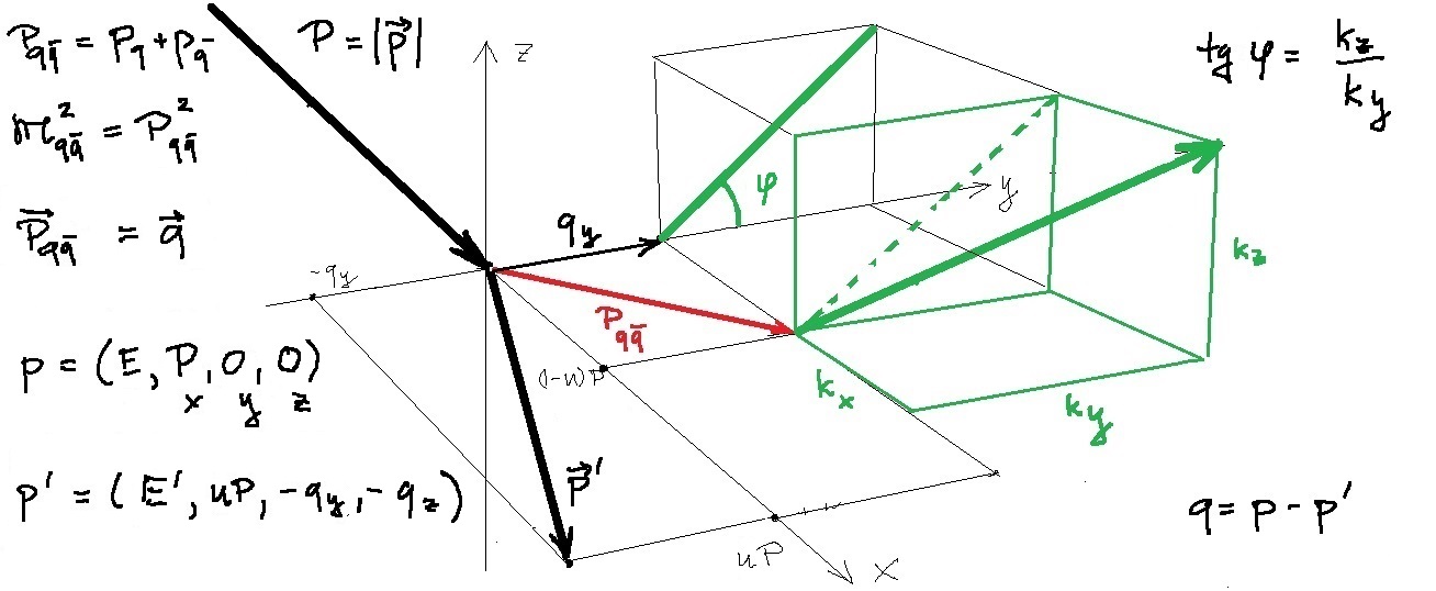
Figure 11: The proton produces a pair in the Fool’s ISR (FISR) frame at LHC. In this example, the proton plane matches the $xy$ plane. The photon emitted by the proton carries the transverse momentum $q_{T}=(q_{y},q_{z})$. The figure is simplified by setting $q_{z}=0$. Generally, $\vec{q}=(q_{x},q_{y},q_{z})=[(1-u)P,q_{y},q_{z}]$, and the outgoing proton carries $\vec{p}\,^{\prime}=(p^{\prime}_{x},p^{\prime}_{y},p^{\prime}_{z})=(uP,-q_{y},-q_{z})$. The relative momentum of a quark with respect to an anti-quark is $\vec{k}$, in the rest frame of the pair. The string between quarks has azimuthal angle $\varphi=\arctan(k_{z}/k_{y})$. For further details, see Sec. IV.

Integration over the pair total momentum renders

$$dP = N_{\rm proton}^{2}2(1-u)\ e_{p}^{2}e_{q}^{2}\Bigg{|}{j^{\mu}\,_{q\bar{q}\,\gamma}\ j_{\mu\ \gamma p^{\prime}\,p}\over(q^{2}-{\cal M}_{q\bar{q}}^{2})\ q^{2}}\Bigg{|}^{2}\delta_{c_{q}c_{\bar{q}}}$$ (34)

$$\times \ {d^{3}k\over(2\pi)^{3}{\cal M}_{q\bar{q}}}\ {d^{3}p^{\prime}\over 2E_{p^{\prime}}(2\pi)^{3}}\ .$$

A sum over colors yields a factor 3 instead of $\delta_{c_{q}c_{\bar{q}}}$. After averaging over initial proton spins and summing over final proton spins and quark spins and flavors, with $e_{p}=1$,

$$dP = N_{\rm proton}^{2}3\sum_{\rm flavor}(e_{q}/e_{p})^{2}\ (1-u)$$ (35)

$$\times {T(x,k^{\perp},p^{\prime},p)\over(q^{2}-{\cal M}_{q\bar{q}}^{2})^{2}\ q^{4}}\ {d^{3}k\over(2\pi)^{3}{\cal M}_{q\bar{q}}}\ {d^{3}p^{\prime}\over 2E_{p^{\prime}}(2\pi)^{3}}\ ,$$

where

$$T(x,k^{\perp},p^{\prime},p) = \sum_{s_{p}}\sum_{s_{q}s_{\bar{q}}s_{p^{\prime}}}\big{|}j^{\mu}\,_{q\bar{q}\,\gamma}\ j_{\mu\ \gamma p^{\prime}\,p}\big{|}^{2}\ .$$ (36)

Evaluation yields

$$T(x,k^{\perp},p^{\prime},p)\,=\,16(F_{1}+F_{2})^{2}\ {\cal T}_{f}$$ (37)

$$- 16\ F_{2}\left[F_{1}+\,{1\over 2}\,\left(1+{q^{2}\over 4m_{p}^{2}}\right)F_{2}\right]\ {\cal T}_{s}\ ,$$

with

$${\cal T}_{f} = 2(t_{1}\,t_{4}+t_{2}\,t_{3})-m_{p}^{2}{\cal M}^{2}_{q\bar{q}}-q^{2}m_{q}^{2}\ ,$$ (38)

$${\cal T}_{s} = 2(t_{1}\,t_{4}+t_{2}\,t_{3})+2(t_{1}\,t_{2}+t_{3}\,t_{4})$$ (39)

$$+ (q^{2}-4m_{p}^{2}){\cal M}_{q\bar{q}}^{2}/2\ ,$$

$$t_{1} = pp_{q}\ ,\ t_{2}\,=\,pp_{\bar{q}}\ ,\ t_{3}\,=\,p^{\prime}p_{q}\ ,\ t_{4}\,=\,p^{\prime}p_{\bar{q}}\ .$$ (40)

The proton form factors $F_{1}$ and $F_{2}$ are parameterized as in Ref. F1F2 .

Using notation $[p^{\prime}]=d^{3}p^{\prime}/[2E_{p^{\prime}}(2\pi)^{3}]$ and Eqs. (23) and (27), the string probability density in the space of vectors $\vec{r}$ is obtained in the form

$$P(\vec{r},p^{\prime},p)\,=\,{dP\over\,d^{3}r}\,=\,[p^{\prime}]\ N_{\rm proton}^{2}\ {3\ \kappa^{6}\over 8\sqrt{8}\ (2\pi)^{3}}\$$ (41)

$$\times \sum_{\rm flavor}{e^{2}_{q}\over e_{p}^{2}}\ {1-u\over{\cal M}_{q\bar{q}}}\ {T(x,k^{\perp},p^{\prime},p)\over(q^{2}-{\cal M}_{q\bar{q}}^{2})^{2}\ q^{4}}\ \theta(L-r)\ .$$

Its magnitude includes the volume of the final proton detector momentum bin, $[p^{\prime}]$. Formally, the same formulas are obtained using the FF and IF of dynamics, except for the difference in direction in the off-shell continuation. The same result holds for electrons, when one sets $F_{1}=1$, $F_{2}=0$ and replaces the proton mass $m_{p}$ by the electron mass $m_{e}$.

The probability $P(\Phi)$ in Fig. 3 is obtained by introducing spherical co-ordinates, $\vec{r}=(r\sin\beta,r\cos\beta\cos\varphi,r\cos\beta\sin\varphi)$ with $\beta=\pi/2-\theta$ and $\theta$ measured from $x$-axis, which is the beam direction, so that $d^{3}r=r^{2}dr\ \sin\theta\ d\theta\ d\phi$. One integrates $\int_{0}^{L}r^{2}dr$ and $\int_{0}^{\pi}\sin\theta\,d\theta$ and sets $\phi=\Phi$.

IV String collisions in $pp$ scattering

We consider peripheral $pp$ scattering that proceeds through photons. In the LHC laboratory frame of reference, the $x$-axis is set along the proton beams, $z$-axis is vertical and $y$ axis is along $\hat{z}\times\hat{x}$.

IV.1 Proton momenta

Initial protons have four-momenta

$$p_{1} = (E,+P,0,0)\ ,$$ (42)

$$p_{2} = (E,-P,0,0)\ ,$$ (43)

with $E=\sqrt{m_{p}^{2}+P^{2}}$. Final protons four-momenta,

$$p^{\prime}_{1} = (E^{\prime}_{1},\ p^{\prime}_{1x},\ p^{\prime}_{1y},\ p^{\prime}_{1z})\,=\,p_{1}-q_{1}\ ,$$ (44)

$$p^{\prime}_{2} = (E^{\prime}_{2},\ p^{\prime}_{2x},\ p^{\prime}_{2y},\ p^{\prime}_{2z})\,=\,p_{2}-q_{2}\ ,$$ (45)

include energies

$$E^{\prime}_{1} = \sqrt{m_{p}^{2}+(P-q_{1x})^{2}+q_{1y}^{2}+q_{1z}^{2}}\ ,$$ (46)

$$E^{\prime}_{2} = \sqrt{m_{p}^{2}+(-P-q_{2x})^{2}+q_{2y}^{2}+q_{2z}^{2}}\ ,$$ (47)

and the azimuthal angles $\Phi_{1}$ and $\Phi_{2}$ of the proton planes

$$\vec{p}\,^{\prime}_{T1} = (-q_{1y},\ -q_{1z})\,=\,p^{\prime}_{T1}(\cos\Phi_{1},\sin\Phi_{1})\ ,$$ (48)

$$\vec{p}\,^{\prime}_{T2} = (-q_{2y},\ -q_{2z})\,=\,p^{\prime}_{T2}(\cos\Phi_{2},\sin\Phi_{2})\ .$$ (49)

The angle $\Phi$ in Fig. 6 equals $\Phi_{1}-\Phi_{2}$. The protons are assumed to lose a sizable fraction of their momentum along the beam, so that the strings have a lot of energy to produce $X$. So, $q_{1x}$ is on the order of $P$ and $q_{2x}$ is on the order of $-P$. Denoting both in-coming protons momenta equally by $p$ and both photon momenta equally by $q$, we have ${p^{\prime}}_{x}=\pm P-q_{x}=\pm uP$ and in the limit $P\to\infty$,

$$q^{2} = -\ {(1-u)^{2}m_{p}^{2}+q_{y}^{2}+q_{z}^{2}\over u}+O(1/P^{2})\ .$$ (50)

IV.2 Quark momenta

In terms of the SRF quark relative momentum $\vec{k}$, the four-momentum of a quark from proton 1 reads

$$p_{q}^{0} = \,{1\over 2}\,\sqrt{{\cal M}^{2}+\vec{q}\,^{2}}+{\vec{q}\cdot\vec{k}\over{\cal M}}\ ,$$ (51)

$$\vec{p}_{q} = \,{1\over 2}\,\,\vec{q}+{\sqrt{{\cal M}^{2}+\vec{q}\,^{2}}\over{\cal M}}\ {\vec{q}\cdot\vec{k}\over\vec{q}\,^{2}}\ \vec{q}+\vec{k}-{\vec{q}\cdot\vec{k}\over\vec{q}\,^{2}}\ \vec{q}\ ,$$ (52)

where $\vec{q}=\left[(1-u)P,\ q_{y},\ q_{z}\right]$ and ${\cal M}=2\sqrt{m_{q}^{2}+\vec{k}\,^{2}}$. Components of the anti-quark four-momentum $p_{\bar{q}}$ are obtained by changing $\vec{k}$ to $-\vec{k}$. The change of sign in front of $P$ provides expressions for quarks coming from proton number 2.

IV.3 Probability $P(\vec{r},p^{\prime},p)$

Given the incoming and outgoing particles’ momenta, elements of probability densities in Eqs. (37)-(40), are

$${\cal T}_{f} = {R_{1}R_{4}+R_{2}R_{3}\over 2x(1-x)u(1-u)^{2}}-m_{p}^{2}{\cal M}^{2}_{q\bar{q}}-q^{2}m_{q}^{2}\ ,$$ (53)

$${\cal T}_{s} = {R_{1}R_{4}+R_{2}R_{3}\over 2x(1-x)u(1-u)^{2}}+{u^{2}R_{1}R_{2}+R_{3}R_{4}\over 2x(1-x)u^{2}(1-u)^{2}}$$ (54)

$$+ (q^{2}-4m_{p}^{2}){\cal M}_{q\bar{q}}^{2}/2\ ,$$

where, using $k=(k_{y},k_{z})$ and $q=(q_{y},q_{z})$,

$$R_{1} = (k+xq)^{2}+m_{q}^{2}+[x(1-u)m_{p}]^{2}\ ,$$ (55)

$$R_{2} = [k-(1-x)q]^{2}+m_{q}^{2}+[(1-x)(1-u)m_{p}]^{2}\ ,$$ (56)

$$R_{3} = (uk+xq)^{2}+u^{2}m_{q}^{2}+[x(1-u)m_{p}]^{2}\ ,$$ (57)

$$R_{4} = [uk-(1-x)q]^{2}+[um_{q}]^{2}+[(1-x)(1-u)m_{p}]^{2}.$$ (58)

Probability $P(\vec{r},p^{\prime},p)$ of Eq. (41) is obtained using Eq. (23) for $\vec{k}$, so that the string vector $\vec{r}=(r\sin\beta,r\cos\beta\cos\varphi,r\cos\beta\sin\varphi)$, where $\beta$ and $\varphi$ are the angle the string forms with the TP and the azimuthal angle measured from $y$-axis, respectively. We have

$$k_{y} = (\kappa^{2}/\sqrt{8})\ r\ \cos\beta\cos\varphi\ ,$$ (59)

$$k_{z} = (\kappa^{2}/\sqrt{8})\ r\ \cos\beta\sin\varphi\ ,$$ (60)

$$x = \,{1\over 2}\,+(\kappa^{2}/\sqrt{8})\ {r\ \sin\beta\over{\cal M}_{q\bar{q}}}\ ,$$ (61)

and ${\cal M}_{q\bar{q}}^{2}=4(m_{f}^{2}+\kappa^{4}r^{\,2}/8)$.

IV.4 Characteristics of string collisionsSRF

Scattering characteristics shown in Fig. 6 are evaluated using Eqs. (7) and (8) and

$${N(\Phi)\over N(0)} = {N(p^{\prime}_{1},p^{\prime}_{2})\over N(p^{\prime}_{10},p^{\prime}_{20})}\,=\,{\tilde{N}_{\rm coll}(p^{\prime}_{1},p^{\prime}_{2})\over\tilde{N}_{\rm coll}(p^{\prime}_{10},p^{\prime}_{20})}\ ,$$ (62)

$${v_{2}(\Phi)\over v_{2}(0)} = {\varepsilon_{2}(p^{\prime}_{1},p^{\prime}_{2})\over\varepsilon_{2}(p^{\prime}_{10},p^{\prime}_{20})}\,=\,{\tilde{\varepsilon}_{2}(p^{\prime}_{1},p^{\prime}_{2})\over\tilde{\varepsilon}_{2}(p^{\prime}_{10},p^{\prime}_{20})}\ ,$$ (63)

where the functions $\tilde{N}_{\rm coll}(p^{\prime}_{1},p^{\prime}_{2})$ and $\tilde{\varepsilon}_{2}(p^{\prime}_{1},p^{\prime}_{2})$ do not contain any constant factors that cancel out in the evaluated ratios. These functions are defined in App. A, Eqs. (A) and (A). Their values result from integration over the range of impact vectors $\vec{b}$, for which strings are capable of slamming into each other, on the features of strings overlap area from Fig. 9, and on the probability distribution of the string vectors $\vec{r}_{1}$ and $\vec{r}_{2}$, over which one integrates in MB averages. For example, strings cannot collide if half of the sum of their lengths is smaller than the length of the impact vector, collisions of thin strings mostly occur through the rhombus shape of Fig. 10, and experimental cuts on multiplicity or elliptic flow limit the azimuthal angle $\gamma$ between vectors $\vec{r}_{1}$ and $\vec{r}_{2}$.

Suppose that strings are chains of effective gluons RGPEPgluons and the volume of a gluon in a chain is $w^{3}$. The corresponding density of gluons is then $\rho=1/w^{3}$. Consequently, the cross-section for inelastic gluon-gluon scattering is $\sigma\sim w^{2}$. The number of gluons in a string of length $r$ much longer than the width $w$, $N_{g}\sim r/w$, is large, which justifies the Glauber-model formula of Eq. (6), which appears in Eqs. (7) and (8) and their computational forms in Eqs. (83) and (84). The rhombus area in Eq. (12) is independent of the impact vector $\vec{b}$ for any sizable $\gamma$. So is the corresponding number of collisions, $N_{\rm coll}(\vec{b},\vec{r}_{1},\vec{r}_{2})$, which makes the exponential in the cross-section take the form $\exp(-c/|\sin\gamma\,|)$, where for the thin strings introduced above the constant $c>1$.

Integration over the impact vectors is illustrated in Fig. 12. For every choice of string transverse lengths $l_{1}$, $l_{2}$ and their relative azimuthal angle $\gamma$, the strings have a non-zero overlap area when the end of vector $\vec{b}$ lies anywhere within a parallelogram of sides $l_{1}$ and $l_{2}$.

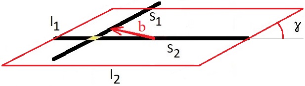
Figure 12: Illustration of the parallelogram in the transverse plane, over which the end of impact vector $\vec{b}$ ranges for some fixed values of the strings lengths $l_{1}$ and $l_{2}$ and their relative azimuthal angle $\gamma$ in the TP. In almost entire parallelogram, the overlap area and its eccentricity are the same when the ratios $w/l_{1}$ and $w/l_{2}$ are negligible. The overlap area is marked in yellow.

For all vectors $\vec{b}$ in the parallelogram, the overlap area and its eccentricity are approximately the same, variations appearing only near the boundaries of the parallelogram and for $\gamma\sim 0$ or $\gamma\sim\pi$. Thus, the parallelogram picture applies in the case of string width $w$ much smaller than the string lengths $l_{1}$ and $l_{2}$. The area of such a parallelogram is $l_{1}l_{2}|\sin\gamma\,|$. Hence, using Eqs. (12) and (13), the thin string approximation for angles $\gamma$ much greater than $\gamma_{0}=2w/l_{1}+2w/l_{2}$ yields

$$\tilde{N}_{\rm coll}(\vec{r}_{1},\vec{r}_{2})$$

$$= l_{1}\,l_{2}\,\left[1-e^{-\sigma(\rho\pi w/4)^{2}\hat{\rho}_{1}\hat{\rho}_{2}w^{2}/|\sin\gamma\,|}\right]\ \ \hat{\rho}_{1}\hat{\rho}_{2}w^{2}\ ,$$

$$\tilde{\varepsilon}_{2}(\vec{r}_{1},\vec{r}_{2})$$

$$= l_{1}\,l_{2}\,|\sin\gamma\,|\left[1-e^{-\sigma(\rho\pi w/4)^{2}\hat{\rho}_{1}\hat{\rho}_{2}w^{2}/|\sin\gamma\,|}\right]\ |\cos\gamma\ |\ ,$$

where the density factor $\hat{\rho}$, is defined in Eq. (89), resulting from Eq. (10).

Note that after integration over impact vectors the MB average number of collisions is not inversely proportional to $|\sin\gamma\,|$, as intuition for small impact vectors suggests. Similarly, eccentricity is not just proportional to $|\cos\gamma\,|$, but rather to $|\sin 2\gamma\,|$. The reason is that both these characteristics include the factor $|\sin\gamma\,|$ that results from integration over impact vectors. Therefore, the MB averaged multiplicity and elliptic flow correlations shown in Fig. 6 result from the inverse of $\sin\gamma$ in the exponential representing the Glauber-model formula.

When $\gamma\to 0$, the Glauber-model exponential tends to zero and the rhombus approximation yields

$$\tilde{N}_{\rm coll}(\vec{r}_{1},\vec{r}_{2}) = \hat{\rho}_{1}\ \hat{\rho}_{2}\ w^{2}\ l_{1}\,l_{2}\ ,$$ (66)

$$\tilde{\varepsilon}_{2}(\vec{r}_{1},\vec{r}_{2}) = l_{1}\,l_{2}\ |\sin\gamma\ |\,|\cos\gamma\,|\ ,$$ (67)

while exact integration for $\gamma=0$, ignoring the exponentials, results in

$$\tilde{N}_{\rm coll}(\vec{r}_{1},\vec{r}_{2})|_{\gamma=0} = \hat{\rho}_{1}\ \hat{\rho}_{2}\ w^{2}\ l_{1}l_{2}\ ,$$ (68)

$$\tilde{\varepsilon}_{2}(\vec{r}_{1},\vec{r}_{2})|_{\gamma=0} = 4(l_{1}l_{2}+w^{2})\arctan(w/l_{1})$$ (69)

$$- 2w(l_{2}-l_{1}+2w)\ .$$

In the limit $\gamma\to 0$, the two results for $\tilde{N}_{\rm coll}$ agree well with each other. In contrast, the rhombus approximation for eccentricity does not extend below the minimal angle order $w/l$ at which the rhombus shape is altered by interference from the ends of strings. The eccentricity formula of Eq. (67), valid for $\gamma\gg\gamma_{0}=2w/l_{1}+2w/l_{2}$, does not automatically match the exact result for $\gamma=0$, with neglected exponentials. Instead, a simple formula achieves the required matching,

$$\tilde{\varepsilon}_{2}(\vec{r}_{1},\vec{r}_{2}) = l_{1}\,l_{2}\ \left(\,|\sin\gamma\,|+\gamma_{0}\right)\ |\cos\gamma|\ .$$

Hence, for general angles $\gamma$, the thin string model provides the following expressions that are used in our estimates

$$\tilde{N}_{\rm coll}(\vec{r}_{1},\vec{r}_{2}) = w^{2}\ (r_{1}+w)\ (r_{2}+w)$$ (70)

$$\times \left[1-e^{-\sigma(\rho\pi w/4)^{2}\hat{\rho}_{1}\hat{\rho}_{2}w^{2}/|\sin\gamma\,|}\right]\ ,$$

$$\tilde{\varepsilon}_{2}(\vec{r}_{1},\vec{r}_{2}) = l_{1}\,l_{2}\ \left(\,|\sin\gamma\,|+\gamma_{0}\right)\ |\cos\gamma|$$ (71)

$$\times \left[1-e^{-\sigma(\rho\pi w/4)^{2}\hat{\rho}_{1}\hat{\rho}_{2}w^{2}/|\sin\gamma\,|}\right]\ .$$

We use these formulas to obtain the ratios shown in Fig. 6 from Eqs. (7) and (8), or their equivalents (62) and (63). The six-dimensional integrals over string vectors $\vec{r}_{1}$ and $\vec{r}_{2}$ are carried out numerically.

IV.5 Beyond minimal bias

A condition of relatively large multiplicity selects events with small values of the angle $\gamma$ in the minimal bias expectation values only through the Glauber cross-section exponential, and not directly through the overlap shape. This is so because the $\sin\gamma$ that results from integration over impact vectors $\vec{b}$ cancels the effect of rhombus overlap area growing like $1/\sin\gamma$ for small angles $\gamma$. In bins of data with large multiplicity, for which the Glauber exponential ought to be small, there also ought to be an increase in elliptic flow.

Indeed, this is what happens according to Eqs. (7) and (8) when one limits the averaging to events with large multiplicities. The resulting effects can be estimated by requiring that the number of binary collisions of Eq. (IV.4) in the events over which one averages is not smaller than a specified fraction $f$ of the maximal observed multiplicity in the peripheral events. According to Eq. (IV.4), this condition reads

$$\tilde{N}_{\rm coll}(\vec{r}_{1},\vec{r}_{2})\geq f\ w^{2}(L+w)^{2}\ .$$ (72)

Computation shows that for $f=1/2$ and $f=0.75$ the multiplicity ratio $N(\pi/2)/N(0)$ decreases from its MB value of about 0.975 in Fig. 6, to about 0.93 and 0.92, respectively. This is nearly a three times bigger oscillation. Correspondingly, the elliptic flow ratio $v_{2}(\Phi)/v_{2}(0)$ drops from its MB value of about 0.965 in Fig. 6 to about 0.90 and 0.875, which is even bigger than a threefold increase in the amplitude.

IV.6 Sensitivity to string features

Our assumed gluon string width $w\sim 0.1$ fm is extremely small. In our estimates, when this is decreased or increased by a factor of three, the multiplicity ratio at its minimum at $\Phi=\pi/2$ does not visibly change. The eccentricity ratio at its minimum decreases by about a percent when $w$ increases in that range.

The upper limit we imposed on the string length, $L=10$ fm, also appears extreme. Reduction of $L$ by half causes an increase of the multiplicity ratio at its minimum to 99% and an increase of the eccentricity ratio at its minimum to about 98%. Thus both azimuthal correlation effects become approximately halved.

Theoretically, when the impact parameter $b$ in a $pp$ ultra-peripheral collision exceeds some value $b_{\rm min}$ larger than the strong-interaction proton diameter, one may exclude from the integration range over $\vec{b}$ in Fig. 12 a circle of radius $b_{\rm min}$. For example, when $b_{\rm min}$ is set to 4 fm, and the product of string lengths $l_{1}l_{2}$ is replaced by $l_{1}l_{2}-\pi b_{\rm min}^{2}>0$, the multiplicity and eccentricity ratios at their minima drop to about 0.93, increasing the string azimuthal effect. This can be interpreted as a consequence of the feature that only long strings can collide for large $b$ and for long strings the azimuthal correlation may be more pronounced than for short ones.

A line of study emerges regarding variation of the multiplicity and elliptic flow ratios with the projectile momentum transfers, such as the variation of Fig. 6 with the photon $q_{1}^{2}$ and $q_{2}^{2}$ in $pp\to ppX$ collisions. For example, when one of the protons referenced in Fig. 6 loses half instead of a quarter of its initial momentum along the beam, which implies that its momentum transfer squared changes from $-1.4$ to $-2.4$ GeV², the ratios of Fig. 6 increase at their minima by about one percent.

IV.7 Comparison with QED lepton-pair production

In our study, the initial stage of a string-string collision resembles photon-photon production of quark pairs. Virtual photons emitted from the beam particles dominate the forward scattering in which one can study string signatures. Key to the formation of these signatures are the initial-stage correlations among the two scattering planes of beam particles and two quark-pair planes. We explain the relevance here of the analogous QED results for the production of two lepton pairs with proton beams. Each virtual photon coming from its respective proton turns into a pair of leptons and the two pairs exchange another virtual photon.

We can infer some preliminary idea of the QED results from Ref. RefA . In the on-shell reaction, $\gamma\gamma\to e^{+}e^{-}+e^{+}e^{-}$, the cross section is dominated by the collinear mass divergences arising from the electron and photon propagator poles. This in turn implies that each pair is close to threshold with little average azimuthal correlation between the pair planes, for unpolarized real photons. This remains true for virtual photons whose average includes the longitudinal mode and whose spacelike mass is small compared to the pair energies. Taking into account the projectile current, on the other hand, we find correlations between the projectile scattering plane and its corresponding lepton-pair plane. What is of primary interest is the correlation between the two lepton-pair planes, and how this correlation depends on the angle between the projectile planes.

Comparison of the string-string collision correlations with QED lepton pair production hinges on the degree to which a photon exchange between lepton pairs and the strong-interaction between quark-pairs differ in their influence on the final-particle distributions. As a benchmark for comparisons, the QED results by themselves are of interest in all of the three cases of proton beams induced, electron beams induced or electron beam and proton beam induced double lepton pair production. Although the QED discussion is beyond the scope of the present paper, we wish to mention that the benchmark estimates can be based on a combination of analytical and numerical calculations as in Ref. RefA or on the event-generator approach as in Ref. RefB . The central need is to identify the data cuts for simulations that allow for comparison with the string model predictions.

V Conclusion

As we have shown in this paper, the physics of ridge production seen in high multiplicity hadronic events in proton-proton collisions at the LHC has important consequences for high energy collisions mediated by photons. This includes ultra-peripheral $pp$ collisions at the LHC, photon-photon collisions at a high energy electron-positron collider, and electron-proton collisions at an electron-ion collider. In each case the virtual photon creates a quark-antiquark pair connected by a gluonic string, i.e., a gluon flux tube.

The gluonic string represents the QCD dynamics of the force which confines the triplet and anti-triplet color of the quark and antiquark. For example, the confining harmonic oscillator potential in the light-front holographic model zeta1 ; zeta2 can be identified with the dynamics of a gluon string.

In the case of an electron at an electron-ion collider, the frame-independent wavefunction of its $|e^{-}q\bar{q}\rangle$ Fock state, defined at fixed light-front time $x^{+}=t+z/c$, is off-shell in $P^{-}=P^{0}+P^{z}$ and thus off-shell in the invariant $q\bar{q}$ mass. The quark and antiquark in the Fock state are confined via the exchange of gluons, the same string-like interactions responsible for color confinement and Pomeron exchange. The virtual state of the lepton becomes on-shell in the electron-proton collision. The high energy collisions of the two flux tubes will produce maximal hadronic multiplicity when the flux tubes are maximally aligned, i.e., when the area of overlap in the transverse plane is maximal as illustrated in Fig. 10. Moreover, as we have shown, the azimuthal distribution of the resulting hadronic ridges will be correlated with the scattering plane of the scattered lepton as illustrated in Fig. 6.

The ratios of multiplicities and elliptic flows shown in Fig. 6 are independent of absolute probabilities or cross sections for the events they concern. The absolute quantities cannot be estimated without using advanced models Baltz . The ratio of cross sections for single tagged versus untagged $pp\to X$ hadronic events at the LHC and RHIC are needed. One needs to estimate the event rate for high multiplicity events in $\gamma p$ collisions and the analogous quantity for the process $pp\to ppX$. High-multiplicity cuts deplete the number of available events by a factor $10^{-6}$ or smaller CMScollectivity in central collisions. In peripheral ones, additional factors of powers of $\alpha\sim 1/137$ significantly reduce the probability to see large number of products in the final state $X$.

However, it is possible to consider replacement of a photon by a pomeron. A string due to a photon from a lepton or a proton may collide with a string due to the pomeron from another proton. Instead of the factor $\alpha^{4}$, one obtains the much larger value $\alpha^{2}$. In such a setup, in analogy to deep inelastic $ep$ scattering illustrated in Fig. 4, one could only seek alignment of elliptic flow with the electron scattering plane. Single-hadron correlation with a projectile plane, in that case a lepton, has already been studied ZEUSazimuthal . However, azimuthal asymmetry of elliptic flow in the final state has to our best knowledge not been measured. If two pomerons replaced two photons, the small factors due to $\alpha$ would be eliminated. However, note that LHC is already considered as a photon-photon collider and software for simulating exclusive production is being built Harland-Lang:2017cax . As far as we know, extension to string collisions due to the photons has not been considered yet.

As a final warning, it should be kept in mind that observable many-body effects due to collisions of gluonic strings are not guaranteed to be describable by many-body techniques used for nucleons in heavy ion physics eccentricity1 ; eccentricity2 ; eccentricity3 . Quarks and gluons are confined objects whose interactions at the distances that characterize their binding mechanism and even the larger distances at which strings may form, are much less understood than the interactions of nucleons are in the context of formation of nuclei and physics of nuclear reactions. Discussion of implications of the string picture for scattering processes that involve ions, including dependence on atomic numbers A and Z from one to the largest available values, would require extension of the theory.

In summary, our estimates for collisions of gluon strings suggest that building required theory and computational tools for absolute estimates should follow experimental verification if the azimuthal variations of multiplicity and elliptic flow do manifest themselves in measurements of ratios exemplified in Fig. 6. Thus, instead of predicting the absolute size of multi-particle string-collision effects, our estimates pose a question of to what extent the correlations of the type illustrated in Fig. 6 do actually occur in proton-proton, lepton-proton or even lepton-lepton scattering. Experimental assessment of their magnitude would motivate directions for developing theory and studying gluon strings using LHC and other machines.

Acknowledgment

The authors thank James Bjorken, Dmitri Kharzeev, Edward Shuryak, Ramona Vogt and Ismail Zahed for discussions. This work is also supported by the Department of Energy contract DE–AC02–76SF00515.

Appendix A Eqs. (7) and (8)

Equations (7) and (8) for average string-collision quantities and Eqs. (62) and (63) for the ratios shown in Fig. 6, involve integration over string vectors $\vec{r}_{1}$ and $\vec{r}_{2}$ as arguments of the string probability densities $P(\vec{r}_{1},p^{\prime}_{1},p_{1})$ and $P(\vec{r}_{2},p^{\prime}_{2},p_{2})$. Since the densities are independent of the impact vector $\vec{b}$, the order of integration in Eqs. (7) and (8) can be changed and multiplicity $N$ and eccentricity $\varepsilon_{2}$ are

$$N(p^{\prime}_{1},p^{\prime}_{2})\,=\,{C_{N}\over\sigma_{\rm p}}\int d^{3}r_{1}\ P(\vec{r}_{1},p^{\prime}_{1},p_{1})$$

$$\times \int d^{3}r_{2}\ P(\vec{r}_{2},p^{\prime}_{2},p_{2})\ N_{\rm coll}(\vec{r}_{1},\vec{r}_{2})\ ,$$

$$\varepsilon_{2}(p^{\prime}_{1},p^{\prime}_{2})\,=\,{1\over\sigma_{\rm p}}\int d^{3}r_{1}\ P(\vec{r}_{1},p^{\prime}_{1},p_{1})$$

$$\times \int d^{3}r_{2}\ P(\vec{r}_{2},p^{\prime}_{2},p_{2})\ \varepsilon_{2}(\vec{r}_{1},\vec{r}_{2})\ ,$$ (74)

where

$$N_{\rm coll}(\vec{r}_{1},\vec{r}_{2})\,=\,\int d^{2}b\left[1-e^{-N_{\rm coll}(\vec{b},\vec{r}_{1},\vec{r}_{2})}\right]$$

$$\times N_{\rm coll}(\vec{b},\vec{r}_{1},\vec{r}_{2})\ ,$$

$$\varepsilon_{2}(\vec{r}_{1},\vec{r}_{2})\,=\,\int d^{2}b\left[1-e^{-N_{\rm coll}(\vec{b},\vec{r}_{1},\vec{r}_{2})}\right]$$

$$\times \varepsilon_{2}(\vec{b},\vec{r}_{1},\vec{r}_{2})\ .$$ (76)

In the ratios shown in Fig. 6 all constant factors cancel out and they can be removed from calculation. With the use of definitions

$$N(p^{\prime}_{1},p^{\prime}_{2}) = C_{N}\ C_{1}\ C_{2}\ \tilde{N}_{\rm coll}(p^{\prime}_{1},p^{\prime}_{2})\ ,$$ (77)

$$\varepsilon_{2}(p^{\prime}_{1},p^{\prime}_{2}) = C_{1}\ \tilde{\varepsilon}_{2}(p^{\prime}_{1},p^{\prime}_{2})\ ,$$ (78)

where $C_{2}=\sigma(\rho\pi w/4)^{2}$ and

$$C_{1} = {1\over\sigma_{p}}2[p^{\prime}_{1}]\ N_{\rm proton}^{2}\ {3e_{p}^{4}\ \kappa^{6}\over 8\sqrt{8}\ (2\pi)^{3}}\ 2[p^{\prime}_{2}]$$ (79)

$$\times N_{\rm proton}^{2}\ {3\ \kappa^{6}\over 8\sqrt{8}\ (2\pi)^{3}}\ .$$

The constant $C_{N}$ is dimensionless, the dimension of $C_{1}$ is mass to the power eighteen, and the dimension of $C_{2}$ is mass squared. Dimensional considerations ought to include the fact that all the observables refer to specific states of final protons and as such are actually densities in the space of final proton momenta, where the measure is $[p^{\prime}_{1}p^{\prime}_{2}]$ of dimension mass to fourth power. The infinitesimal momentum volumes are to be replaced with the experimental ranges of detection of the two outgoing protons. Other factors are: $\sigma$, the parton-parton cross-section; $\rho$, the parton density in a string volume; $w$, the string width; $N_{\rm proton}$, the dimensionless proton-state normalization constant, $e_{p}=1$, the proton charge; and $\kappa$, the holography effective-potential parameter $\sim 0.5$ GeV.

With constants factored out, evaluation of ratios in Fig. 6 can be carried out replacing $N_{\rm coll}(p^{\prime}_{1},p^{\prime}_{2})$ and $\varepsilon_{2}(p^{\prime}_{1},p^{\prime}_{2})$ by

$$\tilde{N}_{\rm coll}(p^{\prime}_{1},p^{\prime}_{2})\,=\,\int d^{3}r_{1}\ \tilde{P}(\vec{r}_{1},p^{\prime}_{1},p_{1})$$

$$\times \int d^{3}r_{2}\ \tilde{P}(\vec{r}_{2},p^{\prime}_{2},p_{2})\ \tilde{N}_{\rm coll}(\vec{r}_{1},\vec{r}_{2})\ ,$$

$$\tilde{\varepsilon}_{2}(p^{\prime}_{1},p^{\prime}_{2})\,=\,\int d^{3}r_{1}\ \tilde{P}(\vec{r}_{1},p^{\prime}_{1},p_{1})$$

$$\times \int d^{3}r_{2}\ \tilde{P}(\vec{r}_{2},p^{\prime}_{2},p_{2})\ \tilde{\varepsilon}_{2}(\vec{r}_{1},\vec{r}_{2})\ ,$$ (81)

where the probability densities without constants are

$$\tilde{P}(\vec{r},p^{\prime},p)\,=\,\theta(L-r)$$ (82)

$$\times \sum_{f}{e_{f}^{2}\over e_{p}^{2}}\ {1-u\over{\cal M}_{q\bar{q}}}\ {T(x,k^{\perp},p^{\prime},p)\over(q^{2}-{\cal M}_{q\bar{q}}^{2})^{2}\ q^{4}}\ ,$$

and

$$\tilde{N}_{\rm coll}(\vec{r}_{1},\vec{r}_{2}) = \int d^{2}b\left[1-e^{-C_{2}\tilde{N}_{\rm coll}(\vec{b},\vec{r}_{1},\vec{r}_{2})}\right]$$ (83)

$$\times \tilde{N}_{\rm coll}(\vec{b},\vec{r}_{1},\vec{r}_{2})\ ,$$

$$\tilde{\varepsilon}_{2}(\vec{r}_{1},\vec{r}_{2}) = \int d^{2}b\left[1-e^{-C_{2}\tilde{N}_{\rm coll}(\vec{b},\vec{r}_{1},\vec{r}_{2})}\right]$$ (84)

$$\times \tilde{\varepsilon}_{2}(\vec{b},\vec{r}_{1},\vec{r}_{2})\ .$$

The functions of impact vector $\vec{b}$ result from integration over the string overlap,

$$\tilde{N}_{\rm coll}(\vec{b},\vec{r}_{1},\vec{r}_{2})$$ (86)

$$= \int d^{2}x_{T}\ \tilde{n}_{\rm coll}(\vec{x}_{T},\vec{b},\vec{r}_{1},\vec{r}_{2})\ ,$$

$$\tilde{\varepsilon}_{2}(\vec{b},\vec{r}_{1},\vec{r}_{2})$$

$$= {[\{x_{T}^{2}\cos(2\alpha)\}^{2}+\{x_{T}^{2}\sin(2\alpha)\}^{2}]^{1/2}\over\{x_{T}^{2}\}}\ ,$$

$$\tilde{n}_{\rm coll}(\vec{x}_{T},\vec{b},\vec{r}_{1},\vec{r}_{2})\,=\,\hat{\rho}_{1}\ \hat{\rho}_{2}$$

$$\times A_{1}(\vec{x}_{T}-\vec{b}/2,\vec{r}_{T1})\ A_{2}(\vec{x}_{T}+\vec{b}/2,\vec{r}_{T2})\ ,$$ (88)

$$\hat{\rho} = {r+w\over(r+w)\cos\beta+w\sin\beta}\ .$$ (89)

References

- (1) S. J. Brodsky, S. D. Głazek, A. S. Goldhaber, R. W. Brown, SLAC-PUB-17106, arXiv:1708.07173 [hep-ph].
- (2) J. D. Bjorken, S. J. Brodsky and A. S. Goldhaber, Phys. Lett. B 726, 344 (2013).
- (3) P. Kubiczek, S. D. Głazek, Lith. J. Phys. 55, 155 (2015); S. D. Głazek, P. Kubiczek , Few-Body Syst. 57, 425 (2016) .
- (4) A. Dumitru, F. Gelis, L. McLerran, R. Venugopalan, Nucl. Phys. A 810, 91 (2008).
- (5) R. Venugopalan, Annals Phys. 352, 108 (2015).
- (6) R. V. Buniy and T. W. Kephart, Phys. Lett. B 576, 127 (2003).
- (7) R. V. Buniy, J. Cantarella, T. W. Kephart, E. J. Rawdon, Phys. Rev. D 89, 054513 (2014).
- (8) K. Johnson and C. B. Thorn, Phys. Rev. D 13, 1934 (1976).
- (9) N. Isgur, J. Paton, Phys. Rev. D 31, 2910 (1985).
- (10) M. L. Miller, K. Reygers, S. J. Sanders, P. Steinberg, Ann. Rev. Nucl. Part. Sci. 57, 205 (2007).
- (11) H.J. Drescher, A. Dumitru, C. Gombeaud, and J.Y. Ollitrault, Phys. Rev. C 76, 024905 (2007).
- (12) D. d’Enterria, G. Kh. Eyyubova, V. L. Korotkikh, I. P. Lokhtin, S. V. Petrushanko, L. I. Sarycheva and A. M. Snigirev, Eur. Phys. J. C 66, 173 (2010).
- Blaizot J P (2014) J. P. Blaizot, W. Broniowski and J.-Y. Ollitrault, Phys. Rev. C 90, 034906 (2014).
- (14) W. Busza and A. S. Goldhaber, Phys. Lett. B 139, 235 (1984).
- (15) J. D. Bowlin and A. S. Goldhaber, Phys. Rev. D 3, 778 (1986).
- (16) P. A. M. Dirac, Rev. Mod. Phys. 21, 392 (1949).
- (17) J. D. Bjorken, S. D. Drell, Relativistic Quantum Fields (McGraw-Hill, 1965); Eqs. (15.28), (17.59) and 17.60).
- (18) G. F. de Teramond, S. J. Brodsky, Phys. Rev. Lett. 94, 201601 (2005).
- (19) S. J. Brodsky, G. F. de Teramond, H. G. Dosch, J. Erlich, Phys. Rept. 584, 1 (2015).
- (20) M. Gell-Mann and M. L. Goldberger, Phys. Rev. 91, 398 (1953).
- (21) A. P. Trawiński, S. D. Głazek, S. J. Brodsky, G. F. de Téramond, H. G. Dosch, Phys. Rev. D 90, 074017 (2014).
- (22) S. D. Głazek, M. Gómez-Rocha, J. More, K. Serafin, Phys. Lett. B 773, 172 (2017) 172.
- (23) R. G. Arnold, C. E. Carlson, F. Gross, Phys. Rev. C 21, 1426 (1980).
- (24) M. Gómez-Rocha, S. D. Głazek, Phys. Rev. D 92, 065005 (2015).
- (25) R. W. Brown, W. F. Hunt, K. O. Mikaelian and I. J. Muzinich, Phys. Rev. D 8, 3083 (1973).
- (26) A. van Hameren, M. Kłusek-Gawenda, A. Szczurek, Phys. Lett. B 776, 84 (2017).
- (27) A. J. Baltz et al., Phys. Rep. 458, 1 (2008).
- (28) CMS Collaboration, Phys. Lett. B 765, 193 (2017).
- (29) ZEUS Collaboration, Phys. Lett. B 481, 199 (2000).
- (30) L. A. Harland-Lang, V. A. Khoze and M. G. Ryskin, arXiv:1709.00176 [hep-ph].
- (31) P. F. Kolb, J. Sollfrank, U. W. Heinz, Phys. Rev. C 62, 054909 (2000).
- (32) PHOBOS Collaboration (B. Alver et al.), Phys. Rev. C 77, 014906 (2008).
- (33) D. Teaney and L. Yan, Phys. Rev. C 83, 064904 (2011).