Background-Limited Imaging in the Near-Infrared with Warm InGaAs Sensors:
Applications for Time-Domain Astronomy

Abstract

We describe test observations made with a customized $640\times 512$ pixel Indium Gallium Arsenide (InGaAs) prototype astronomical camera on the 100″ DuPont telescope. This is the first test of InGaAs as a cost-effective alternative to HgCdTe for research-grade astronomical observations. The camera exhibits an instrument background of 113 e-/sec/pixel (dark + thermal) at an operating temperature of -40C for the sensor, maintained by a simple thermo-electric cooler. The optical train and mechanical structure float at ambient temperature with no cold stop, in contrast to most IR instruments which must be cooled to mitigate thermal backgrounds. Measurements of the night sky using a reimager with plate scale of $0.4$″/pixel show that the sky flux in $Y$ is comparable to the dark current. At $J$ the sky brightness exceeds dark current by a factor of four, and hence dominates the noise budget. The sensor read noise of $\sim 43e^{-}$ falls below sky+dark noise for exposures of $t>7$ seconds in $Y$ and 3.5 seconds in $J$. We present test observations of several selected science targets, including high-significance detections of a lensed Type Ia supernova, a type IIb supernova, and a $z=6.3$ quasar. Deeper images are obtained for two local galaxies monitored for IR transients, and a galaxy cluster at $z=0.87$. Finally, we observe a partial transit of the hot Jupiter HATS34b, demonstrating the photometric stability required over several hours to detect a $1.2\%$ transit depth at high significance. A tiling of available larger-format sensors would produce an IR survey instrument with significant cost savings relative to HgCdTe-based cameras, if one is willing to forego the $K$ band. Such a camera would be sensitive for a week or more to isotropic emission from $r$-process kilonova ejecta similar to that observed in GW170817, over the full 190 Mpc horizon of Advanced LIGO’s design sensitivity for neutron star mergers.

1 Introduction

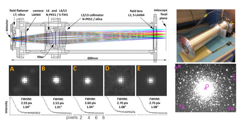
Figure 1: Photograph of the InGaAs reimaging camera assembly (upper right) and cross-sectional view of the lens configuration (upper left). The DuPont telescope focal plane is to the right of the field lens, and the sensor is located at left. The camera requires only boas voltages, separate power for the backing TEC, and USB3 (which is converted and transmitted over fiberoptic lines to the control room). Bottom row indicates PSF image quality across the field, measured using the globular cluster shown at bottom right for indicated field positions.

The high cost of infrared sensors has limited the size of focal plane arrays for infrared sky surveys, despite the demand for this capability to complement optical surveys now underway or planned (Law et al., 2009; Bellm & Kulkarni, 2017; LSST Science Collaboration et al., 2009). InGaAs focal planes offer a lower-cost alternative to heritage designs based on HgCdTe, and sensors are available with $15\mu$m pixels in up to 2k$\times$1k format.

The red cutoff for standard commercial InGaAs material is at $\sim 1.65\mu$m. Cameras made with these sensors only operate in the $Y,J$, and short $H$ bands. Owing to the lack of $K$-band sensitivity, these cameras can be operated at higher temperature thus relaxing requirements on sensor and instrument cooling. In addition, InGaAs has lower dark current than HgCdTe at fixed temperature (Beletic et al., 2008), further facilitating warm operation.

Because InGaAs sensors are typically designed for high-background and video applications, most commercially available cameras are not suitable for astronomy research. The high dark current from ambient temperature operation, coupled with read noise measured in hundreds of e- (RMS) compromises on-sky performance. Some vendors are pushing the noise envelope by either targeting low dark current from cooling, or low read noise, but commercial cameras presently do not feature both low dark current and low read noise simultaneously in a large format. Specifically, none of the commercial cameras utilize non-destructive reads to take advantage of Fowler (Fowler & Gatley, 1990) or up-the-ramp sampling (Chapman et al., 1990) as is common in astronomical research-grade cameras.

Recently, progress in material growth has yielded sensors with lower dark current that are packaged with integrated thermoelectric coolers (TECs) to lower the noise floor. To miticate read noise, we have built a camera with a 640$\times$512 pixel InGaAs sensor, and implemented non-destructive reads via a custom daughter board and FPGA to mitigate read noise. Our laboratory measurements indicate that this system should achieve sky-background limited noise performance on a 1-meter telescope with 1″ pixels, or larger telescopes with smaller pixels in the $J$ and $H$ bands, and marginally for $Y$ as well.

This report describes on-sky performance tests of this prototype camera on the 2.5-meter DuPont telescope at Las Campanas Observatory, Chile. During the course of a 3-night engineering run during November 2016 bright time, we mounted the camera with a small set of reimaging optics to measure broadband sky backgrounds, obtain photometric zero points, test imaging depth and photometric stability. We observed several IR transients as well as faint static sky targets to demonstrate possible science applications of an imager in this configuration. Based on experience with this system we project the performance of warm InGaAs imagers for selected science appliations.

2 Sensor Selection

All tests described here were made with a 640$\times$512 AP1121 sensor from FLIR electro-optical components. This is very similar to the APS640C camera described in Sullivan et al. (2013), but with 15$\mu$m rather than $25\mu$m pixels(Sullivan et al., 2014; Sullivan, 2015). The dark signal continues to drop as the temperature is lowered, to the $-45$C limit of tests with our apparatus.

The AP1121 has an electronic shutter and CTIA pixel architecture, unlike the HAWAII family whose pixels have source-follower amplifiers (Beletic et al., 2008). We run the AP1121 at high frame rate and average multiple frames using sample-up-the-ramp mode to reduce read noise.

Primary cooling power for the sensor is derived from the thermo-electric cooler (TEC) integrated into its package. The InGaAs substrate and ROIC are protected by the package’s vacuum seal, which admits light through an AR-coated sapphire window. In our camera head, the warm side of the on-sensor TEC abuts a copper post, which has a secondary high-capacity “backing” TEC on its opposite side, powered by a dedicated supply. The warm side of the backing TEC mates to a standard CPU water cooling block, of the variety seen in many gaming or overclocked PCs. Standard 0.75-inch Buna-N hoses connect the cooling block to a ThermoTek recirculating bath chiller. We run the bath with distilled water at +5C, which cools the TEC but did not result in condensation on hoses or within the camera head. To mitigate condensation on the window of the sensor package, we run a N₂ gas line into the camera head with a regulator to provide a gentle positive flow of dry air.

This design does not maintain the sensor package in vacuum, nor does it achieve deep cooling, since the TEC stack implementation (which employs an long thermo-mechanical path) is very inefficient. However it did allow us to operate the camera in the range of $T=-40$ to $-45$C, adequate for our testing purposes.

3 Reimaging Camera and Filters

To resample the focal plane into a scientifically realistic configuration, we assembled a modest reimaging camera that converts the plate scale of the 100-inch DuPont telescope from its native value of 0.16″ per pixel to 0.4″. This provides Nyquist sampling for all but the best seeing conditions at Las Campanas, and is set as coarse as is practical to mimic the field-of-view requirements for a wide-field survey instrument. The overall field of view of the 640$\times 512$ sensor is 4.3′$\times$3.4′.

The reimager optics (Figure 1) begin with a 72mm diameter (clear aperture) plano-convex field lens, which circumscribes the projected field of view on the telescope focal plane and defines a pupil location inside the barrel near the filters. The diverging beam is collimated by a doublet of diameter 58mm, just prior to the optical pupil.

Notably, this configuration has no cold Lyot stop—the optics are completely warm and float at ambient temperature. Such a design could easily accommodate a stop if one were desired, but we will demonstrate below that the $K$-blind nature of the InGaAs sensor makes the instrument sky-noise dominated.

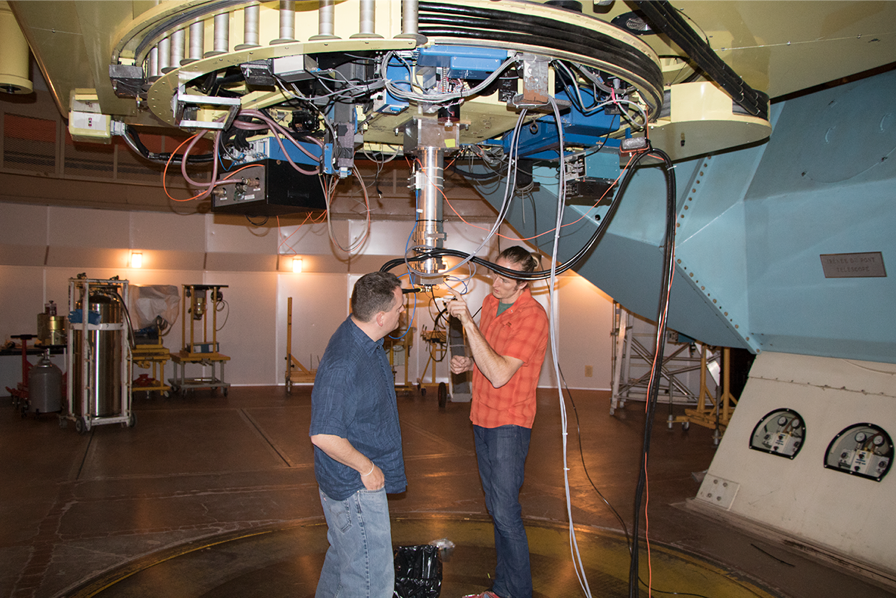
Figure 2: InGaAs prototype camera mounted on the DuPont telescope’s Instrument Mounting Base. Buna-N coolant hoses and fiber-optic interface are draped at right from the port, the gray cables bring power for the sensor and thermo-electric backing coolers.

Our MKO-$Y$ and $J$ band filters (Tokunaga et al., 2002) mount just beyond the pupil in a detent-indexed slide, which tilts the filters by 2 degrees to avoid ghosting. Because our sensor substrate is classical InGaAs material and is not prepared for extended-blue sensitivity (due to cost and availability) there is a slight throughput loss from QE rollover at the bluest edge of the $Y$ band, but this has only a small effect on overall sensitivity. Although InGaAs is also photosensitive over much of the $H$ band, we did not test in this region because our main goal was to establish whether the camera would be background-limited, and we were confident that it would be in $H$ because of the much brighter sky emission.

A 50 mm diameter doublet is used in conjunction with a plano-convex singlet and field flattener to refocus the beam onto the sensor at the desired pixel scale. All lenses were treated with broad-band anti-reflection coatings from Evaporated Coatings, Inc.

The lenses were bonded into precision-machined bezels using RTV60. Each of the lens groups contained one plano surface to simplify axial registration against datum surfaces on the bezels. Laboratory test images taken with a USAF target placed at the location of the DuPont focal plane verified full MTF contrast at line spacings of 71$\mu$m (0.77″) and partial contrast at 62$\mu$m (0.67″) for a projected pixel scale of 37$\mu$m. This indicates that image quality is limited by the telescope and sensor commbination, and aberrations from the camera contribute at the $<1$ pixel level. Astrometric calibration of images on the sky yield an as-built pixel scale of 0.396″(design is 0.4).

We shipped the camera to Las Campanas Observatory fully assembled, and bolted to the standard Instrument Mounting Base of the DuPont so as to use the observatory guiders during the night. We placed the chiller on the dome floor and draped cables from hard points on the telescope. The cables included a USB3-to-fiber converter which ran to our control laptop in the control room. We located all power supplies in the control room, with long cable runs to the instrument port, to facilitate diagnostic monitoring and power cycles if needed.

4 Detector Performance

4.1 Dark Current

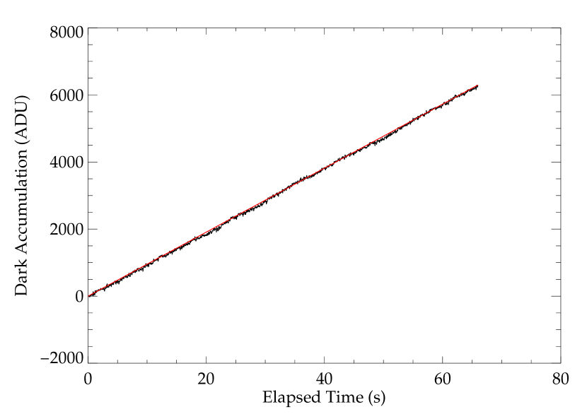
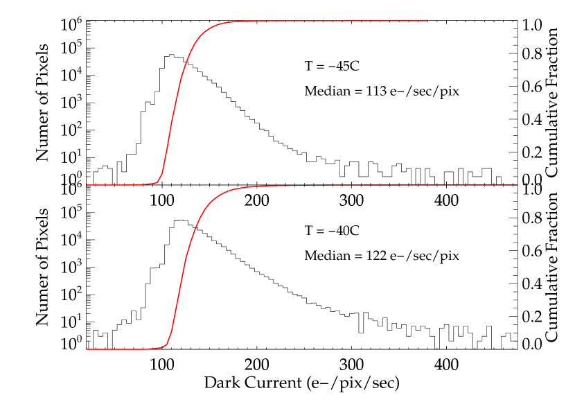
Figure 3: (Left) Example of a dark current ramp fit for a single pixel at $T=-45C$, accumulating at approximately 100 counts/second. Black represents measured counts, with the linear fit shown as a red solid line. (Right) Dark current measurements in e-/sec as mounted on the telescope.

We obtained measurements of the combined background from sensor dark current and thermal emissivity by closing the dome and mirror covers during nighttime hours and taking one-minute ramps with 1200 samples. After correcting these frames for linearity, we performed a linear fit of the dark count slope versus time for each pixel on the array. Figure 3 shows an example of one such fit for a single pixel in the left panel, and the right panel shows statistics of the per-pixel dark current across the array, assuming a gain of 1.17 e-/ADU as measured previously in the lab (Sullivan, 2015).

We operated our first two nights at $T=-40$C and the third night at $T=-45$C, and measured the dark current at both temperatures. The median dark current at the lower temperature is 113 e-/sec/pixel. A high-end tail is visible and most prominent at the array corners; this tail is suppressed at colder temperatures, and 90% of pixels have a dark value of $\leq 140$ e-/sec as seen in the red cumulative histogram.

This measured dark current is high relative to cryogenically cooled HgCdTe. However at equivalent temperature ($T=-40$C) and pixel size, commercial 1.6$\mu$m-cutoff HgCdTe would have a much higher dark level of 100,000 e-/sec/pixel (Beletic et al., 2008), and $2.5\mu m$ HgCdTe would be higher yet. This is the fundamental factor enabling use of InGaAs for lower cost warm instruments. Our prior laboratory measurements indicate that further reduction in dark current is possible at lower operating temperature, allowing one to tailor dark current to different site conditions through straightforward thermal engineering.

4.2 Read Noise

We did not measure read noise separately at the telescope, but instead used laboratory values taken prior to on-sky deployment. Using flat fields taken at varying illumination levels below the full-well (corrected for non-linearity), we calculated the conversion gain from the slope at 1.17 e-/ADU by regressing signal variance against mean. Extrapolating this fit to zero mean flux, we obtained a single-sample read noise of 59 e- RMS.

The delivered read noise is reduced substantially through non-destructive sampling. For up-the-ramp integrations of 64 samples we measure read noise of $43e^{-}$ RMS; during on-sky operations we always operated in SUTR mode, and except for bright standard stars our ramps always exceed 16 reads, keeping read noise within this bound. For comparable read noise values, Poisson noise from dark+sky counts overtakes read noise within a 7 second exposure in $Y$ and 3.5 seconds in $J$, using the sky brightness estimates measured as described below.

4.3 Linearity

Non-linearity is a known issue with all IR sensors and our previous measurements in the lab revealed non-linearity at the $\sim 3-5\%$ level, varying across the sensor. We calibrate out nonlinearity using flat field ramps run to saturation at the start of the observing run. For each pixel, we fit a 4th order polynomial to the residual counts relative to a straight linear fit, regressing the residuals against count rate over the first 35,000 counts in each pixel. We store the polynomial coefficients for each individual pixel and correct each science and calibration frame as the first step in data reduction (before calculating the SUTR slope).

This method reduces the residual observed non-linearity to $\sim 0.5\%$ or less (Figure 4). There is evidence in the residuals that a higher order polynominal could reduce nonlinearity yet further, at the risk of over-fitting. We also observe a higher non-linearity near the start of our ramps (i.e. 1% at the first sample), but the array is essentially never operated in this regime because of robust dark current and sky backgrounds.

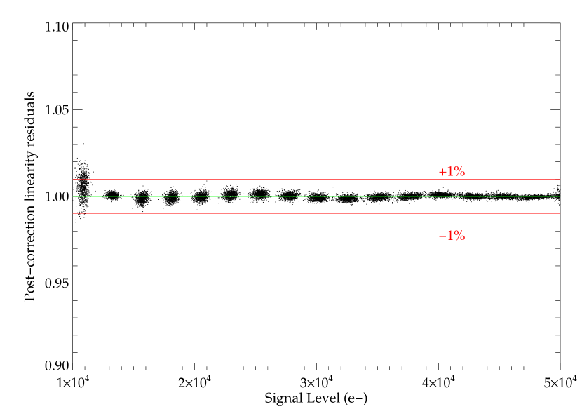
Figure 4: Residuals of an individual flat field exposure relative to a straight linear fit, after performing a fourth-order polynomial nonlinearity correction. Slightly higher residuals are measured at low count rate, but the sensor is essentially never run in this regime because of robust thermal and sky backgrounds.

4.4 Data Reduction

Data from the camera are stored as SUTR FITS arrays containing individual reads from each sensor reset. A small set of IDL routines is used to correct for non-linearity in the counts and then calculate the SUTR slope as described in Benford et al. (2008). The output is expressed in terms of e-/second. The non-linearity correction is critical for maintaining uniformity of the background counts, as the size of the correction varies coherently across the array.

We then subtract a dark current frame (also in e-/second) compiled as described above. The remaining flux from the sky and sources is normalized by a flat field composite constructed from stacked twilight sky exposures taken with the DuPont. The flat field reference is corrected for non-linearity and dark current, and normalized by the median count rate to derive a unity-median calibration frame that is divided into the science frame’s count rate. Individual pixels showed gain variations of 1-5% relative to the median value.

For fields requiring deep photometry, we combined multiple exposures taken at different telescope dither positions. We used the fitsh processing software (Pál, 2012), which matches and registers the images to a common reference using direct photometry of (sometimes faint) stars.

We subtracted a spatially constant background flux from each image and applied an overall scaling to match fluxes between exposures. The final composite was constructed from a median of the registered, background-subtracted, and flux-scaled frames. No weights were applied for the average since a median rather then mean was used for the operation. Finally, we reapplied approximate absolute astrometric solutions generated by the Scamp and Swarp packages (from astr0matic.net) to the final stacks for future convenience.

5 On-sky Performance

The configured camera was used during three engineering nights on UT 2016 November 11, 12, and 13.

5.1 Sky Backgrounds

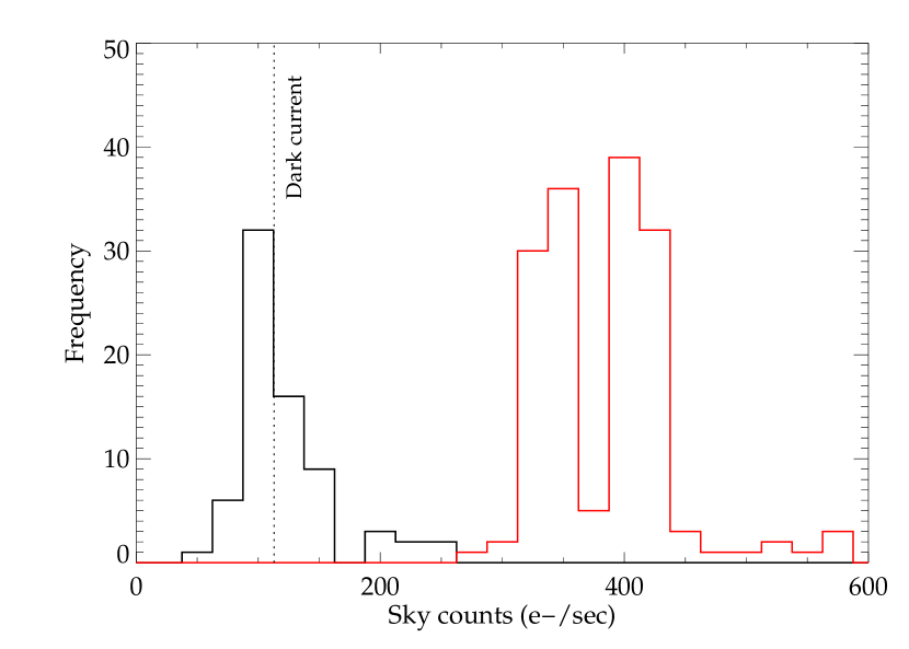
Figure 5: Histogram of median sky counts observed in individual frames taken on the DuPont. The black histogram depicts the $Y$ band sky and red curve indicates $J$ background. Dotted line indicates the measured dark current at $T=-45$C. $J$ band observations are well into the sky-limited regime, while Poisson noise from the dark current and sky contribute roughly equally to the total noise budget in $Y$. This can be mitigated through colder operation or a coarser pixel scale.

We gathered statistics on the sky backgrounds by recording the median count rate for every exposure taken during the run, in each filter. A histogram of these values is shown in Figure 5.

The Y band background is characterized by a unimodal distribution centered around a median count rate of 103 counts/sec/pixel, or 121 $e^{-}$/sec/pixel. This is nearly identical to the measured dark current at $-40$C and slightly higher than the dark rate for $-45$C, indicating that we are nearly sky-noise limited even the band with the darkest sky.

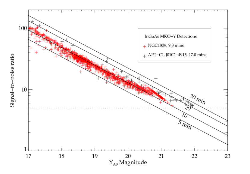
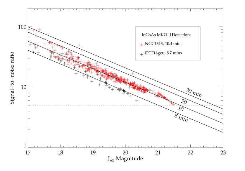
Figure 6: Photometric depth, displayed as signal-to-noise ratio over apparent magnitude in three fields with different filters and exposure times. The SNR is calculated from the isophotoal fluxes (and errors) of objects measured with Sextractor.

Table 1: On-Sky InGaAs Prototype Performance

Quantity	$Y$ value	$J$ value
Zero point (1 e-/sec)	24.53	25.27
Sky background (e-/sec/0.4′′ pixel)	120	413
Sky background (mag/sq. arcsec)	17.5	16.8
Dark+thermal background (e-/sec/pixel)	113	113

The $J$ band sky counts are bimodal, because some of our pointings were quite close to the moon. The median $J$ sky flux was 352 counts/sec/pixel, or 412 $e^{-}$/sec, a factor of $\sim 4$ higher than the dark current. Observations in $J$ (and by extension, $H$ as well) will be dominated by Poisson noise from the sky, with some margin.

We estimated a calibration of the night sky brightness using observations of the spectrophotometric standard star Feige 110 taken during nights 2 and 3 of the run. Using data from the CALSPEC archive at STScI and measured transmission curves of our filters supplied by vendors, we estimated the bandpass center of each filter and compared with measured count rates to establish photometric zero points. The measured zero points and sky backgrounds are reported in Table 1.

From these calibrations, we estimated the median $Y$-band sky surface brightness at 17.45 AB magnitudes per square arcsecond, which may be compared with the measured value of 17.50 determined at the same site for Magellan/FourStar (Persson et al., 2013). Likewise the $J$ band surface brightness is 16.84 AB magnitudes per square arcsecond, compared to 16.90 measured by FourStar.

There remain systematic uncertaintes in our calibration from not accounting the detailed sensitivity curve of the instrument or variation in the SED of the standard star across each filter bandpass. These calculations merely indicate that our zero points and methodology produce consistent answers with other instruments at the same site with established heritage. Importantly, they also indicate the possibility of achieving largely sky-limited noise performance using a warm optical train with no Lyot stop, and a modestly-cooled sensor.

If one wishes to obtain a more favorable noise budget, then further sensor cooling should result in even lower dark current values (Sullivan, 2015). Alternatively, adaptation of the optical design to deliver 0.5″pixels rather than 0.4″would increase the sky background by 50% and cover a wider field. This must be traded against the desire to properly sample seeing and achieve maximum point source sensitivity.

5.2 Photometric Depth

We compiled imaging data on multiple fields with differing depths as we exercised the instrument in various configurations and settled on observing strategies. Because the camera is background limited, the SNR should scale as $\sqrt{t}$, but a goal of the run was to establish the baseline for this scaling.

In Figure 6 we show photometry for two fields apiece in $Y$ and $J$. The measurements are generated using Sextractor (Bertin & Arnouts, 1996) with a detection threshold of $5\sigma$ yielding object catalogs of object isophotal AB magnitudes (uncorrected for aperture), which we plot against SNR. A regression on the 10-minute exposure photometry (for NGC1809 in $Y$ and NGC1313 in $J$, shown as solid lines) confirms that sensitivity scales approximately as $\sqrt{t_{exp}}$ as expected for other fields observed at different depth.

The shallower slope of the $J$ band curves reflects the higher sky background, but the overall sensitivity is similar because of the sensor’s higher QE in $J$, and correspondingly higher zero point. Both filters reach a limiting magnitude of approximately $AB=21$ in 5 minutes, $AB=21.5$ in 10 minutes, and $AB=22-22.4$ in 20 minutes.

For our $J$ band observations, we cross-checked our photometry calibrated with Feige 110 against 2MASS (Skrutskie et al., 2006) stars in the field and adjusted the zero points to bring the two into agreement. Typically these corrections were $\sim 0.05$ magnitudes except in one case where we observed $0.15$ magnitudes of extinction from clouds. For $Y$ we did not have a photometric reference catalog covering observed fields and used our Feige110 calibrations without correction.

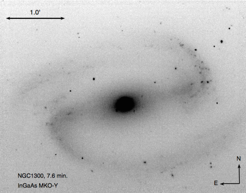
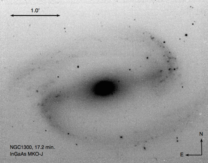
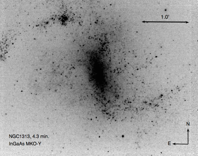
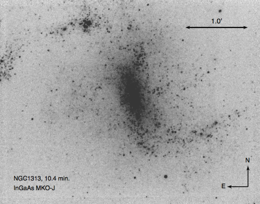
Figure 7: Y and J images of nearby galaxy NGC1300 (top row) and the SPIRITS survey target NGC1313 (bottom row).

A more sophisticated estimate of sensitivity or completeness could be made by injecting simulated objects into the data and testing the efficacy of Sextractor at recovering these objects. However the present analysis provides a sufficiently general estimate of photometric speed to evaluate potential survey science programs, described below.

5.3 Representative Science Observations

We observed several selected science targets chosen to represent a range of possible observational programs that would benefit from background-limited IR photometry in the $Y$ through $H$ bands at reduced cost and complexity. These specifically include (a) observations of nearby galaxies typical of astrophysical transient searches, (b) deep images of fields at cosmological distances to search for distant quasars and clusters, and (c) observations of transiting exoplanets in the near-infrared.

5.3.1 Nearby Galaxies, including IR Transient Survey Objects

We observed two galaxies from the local universe: NGC1300 and NGC1313 (Figure 7). The latter object in particular was targeted because it is used for a synoptic IR survey of obscured transients using the Spitzer Space Telescope. NGC1300 was observed for 7.6 minutes in $Y$ and $17.2$ minutes in $J$, whereas NGC1313 was observed for 4.3 and 10.4 minutes in the same filters, respectively. The unusual exposure times reflect rounding to the nearest clock time for an even number of ramp frames, and were varied throughout the run as we refined our observing strategy.

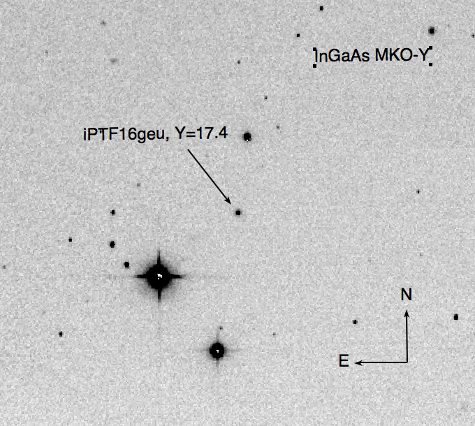
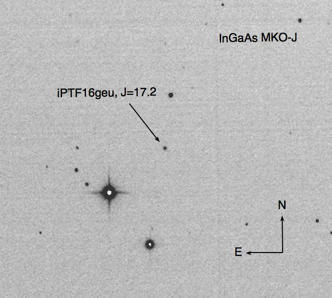
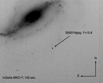
Figure 8: $Y$ (left, 391 seconds) and $J$ (center, 326 seconds) band images of the gravitationally lensed Type Ia supernova iPTF16geu. At right is a Y band image of SN2016gkg (152 seconds).

5.3.2 Supernovae and Explosive Transients

A primary motivation for building a wide-field IR camera is to pursue time-domain science in the $Y$ through $H$ bands. Accordingly, we observed two supernovae that were visible during the run as a demonstration.

Our first target was iPTF16geu, a gravitationally lensed Type Ia supernova (Goobar et al., 2017). Figure 8 shows $Y$ and $J$ band images of the field, with 391 and 326 second integrations, respectively, taken on 2016 November 13 (UT00:22:27 for $Y$ and UT00:53:58 for $J$). We measure a total apparent magnitude of $Y_{AB}=17.4$ at $55\sigma$ significance, and $J_{AB}=17.2$ at $38\sigma$. Although the data were taken in good seeing conditions, we were not able to resolve individual components of the lens.

Our other supernova target is the Type IIb source SN2016gkg (Bersten et al., 2018), observed 152 seconds in $J$ and 206 seconds in $Y$ (Figure 8). We detect the supernova with $Y_{AB}=15.9$ at $214\sigma$ and $J_{AB}=16.12$ at $205\sigma$.

5.3.3 High-Redshift QSOs

A key static-sky application for near-IR imagers is the search for high redshift QSOs in deep data sets. To test whether the InGaAs sensor is sensitive to currently known high-$z$ populations, we observed the known $z=6.31$ quasar ATLAS J025.6821-33.4627 (Carnall et al., 2015). This object was (somewhat unusually) selected from $z-W1$ (WISE) colors, so its near-IR magnitudes were not reported in the literature.

Figure 9 shows a cutout of the $J$ band image, which was observed for 326 seconds. We detect a source at the expected location of the QSO with $J_{AB}=18.91$ and $20\sigma$ significance. The quasar was also observed for 717 seconds in $Y$ and a source is clearly visible in the data. However poor image registration (caused by a low star count in the high-latitude field) complicates photometry and requires further refinement to produce a well-calibrated measurement.

5.3.4 Faint/High-Redshift Galaxies and/or Clusters

To push photometric depth, we constructed a 17-minute $Y$-band stack of the field containing the $z=0.87$ galaxy cluster ACT-CL J0102-4915 (nicknamed “El Gordo”; Menanteau et al., 2012). Using the zero points listed in Table 1, we extracted magnitudes for all sources detected with $\geq 5\sigma$ signifiance—these are circled in Figure 10. Although the extremely luminous Brughtest Cluster Galaxy (BCG) is well above the noise floor at $Y\approx 18$, we also detect numerous objects from the red sequence at $y=21.5-22.5$, our approximate detection limit.

This observation, together with the $z=6.3$ QSO observations presented in 5.3.3 suggests that wide-field InGaAs mosaics can deliver sufficient imaging depth to survey, discover and charaterize objects at cosmological distances.

5.3.5 Exoplanet Transit

Our early studies with InGaAs were partially motivated by an interest in using the sensors for exoplanetary transit surveys around low-mass stars, including L and T dwarfs which are bright in the $J$ band. Our earlier work (Sullivan et al., 2013, 2014) included laboratory tests of photometric stability, but did not present on-sky detections of transit events.

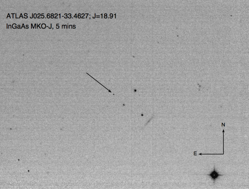
Figure 9: Image of the $z=6.31$ quasar ATLAS J025.6821-33.4627. This source is clearly detected at $20\sigma$ signficance for $J_{AB}=18.91$ in a $\sim 5$ minute integration.

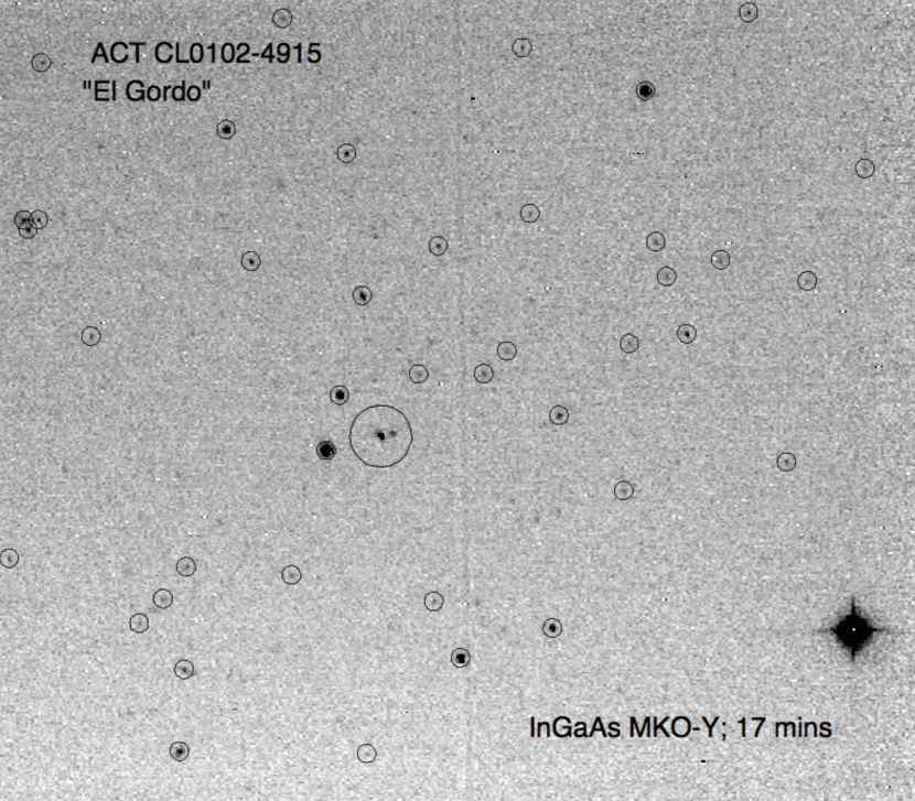
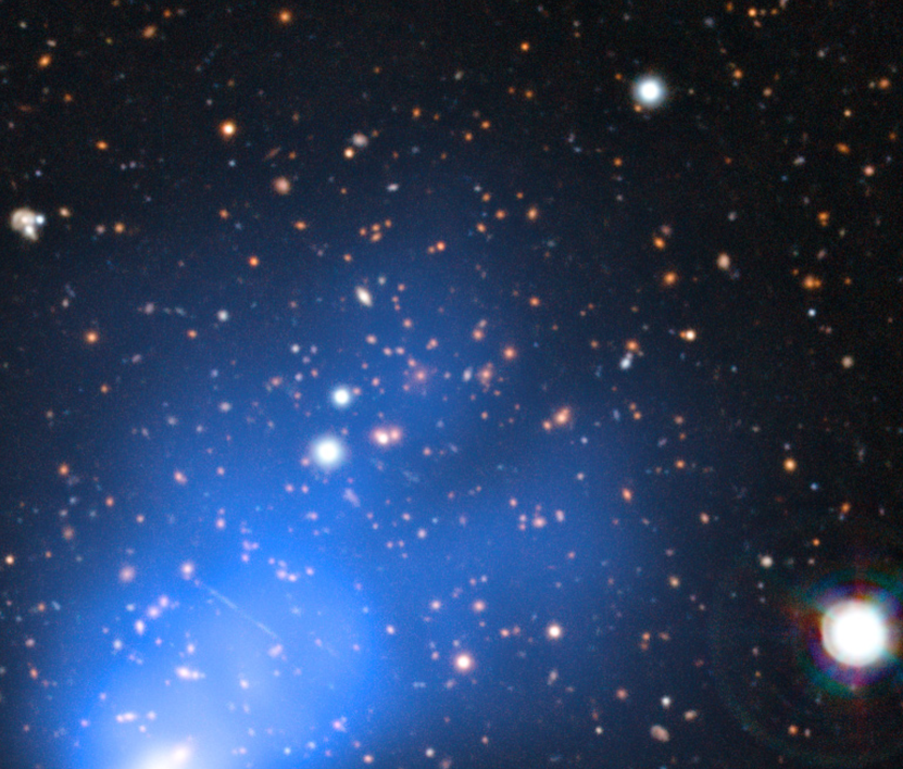
Figure 10: Left: 17 minute $Y$ band image of the galaxy cluster ACT CLJ0102-4915 (Menanteau et al., 2012, “El Gordo”) at $z=0.87$. The Brightest Cluster Galaxy is indicated at center, and has $Y\approx 18$. The majority of the other $5\sigma$ detections indicated are at $Y\approx 21.0-22.5$. Right: Optical image of the same field with VLT/SOAR for reference, with Chandra map overlaid in blue (Menanteau et al., 2012).

We did not schedule the DuPont run explicitly for optimal observation of an exoplanet transit, but a database search revealed a small number of partial transits which were visible from Las Campanas during our run. Because of the InGaAs camera’s small field size, we focused our search on targets with bright nearby comparison stars.

We observed the newly discovered Hot Jupiter HATS34b, a 0.94 Jupiter-mass planet orbiting a $V=13.9/J=12.5$ (Vega) host star of $T_{eff}=5380$K. The object orbits with $P=2.1$ days and was visible through ingress and transit during last portion of the night. Its field includes a second comparison star 2.5 magnitudes brighter than HATS34, at a projected distance of 163″. Sunrise prevented observations of the transit egress and re-establishment of a post-transit photometric baseline. The transit depth reported in the discovery paper (de Val-Borro et al., 2016) is 13.4 mmag, or 1.2%.

So as not to saturate either star, we obtained short individual exposures of $t=1.03$ seconds, with the telescope slightly defocused. The telescope was guided throughout the sequence by an off-axis probe provided by the observatory, to maintain stable positioning of objects on the array.

We extracted fluxes of the science target and reference star using Sextractor in strict aperture photometry mode, with an aperture diameter of 15 pixels (6″). No attempts were made to optimize the photometric extraction parameters or aperture.

Figure 11 shows the resulting lightcurve, constructed from differential photometry between the target and reference stars. To reduce shot noise, we bin the counts from multiple exposures by adding the photometric fluxes with a top hat window of varying width, to verify the scaling of noise reduction. We center around the known time of transit calculated from the HATS34b discovery paper. The black solid points are averages of 11 exposures, or 11.33 seconds, whereas the red points average 80 exposures for 82.4 seconds.

Even in the 11 second averages, there is a clear transit detection with a depth consistent with the value reported by the HATS team (the expected optical transit depth is indicated with a light green line). In the 82-second bins the detection is highly significant, with a transit depth slightly larger than the 1.2% predicted by HATS, but within the margin of error.

Our main objective was not to fit a new transit lightcurve and re-derive the orbital properties of HATS34b. We simply demonstrate that InGaAs sensors are capable not just of deep photometry and detection of explosive transients, but also of precision photometry at the milli-magnitude level, over long time baselines. These data were obtained in the $J$ band where the sky is brighter and more variable in emission and transparency than the optical. It suggests that with proper attention to noise, stability, and observation InGaAs cameras can offer an affordable alternative to costly HgCdTe arrays for IR transit observation—particularly if a large format is not required.

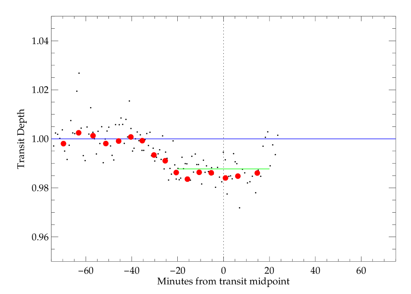
Figure 11: $J$ band light curve of HATS-34b recorded over the partial transit of UT2016 November 12. Black dots indicate 11-exposure bins, for effective exposure time of 11.33 seconds. The solid red cirles are more heavily binned into intervals of 82.4 seconds.

6 Discussion

6.1 Suitability for Synoptic Infrared Kilonova Surveys or LSST Synergy

Wide-field near-IR imagers are potentially attractive survey instruments to search for and characterize the electromagnetic (EM) counterparts of binary neutron star (BNS) mergers detected via gravitational waves. Pioneering work by Li & Paczyński (1998) and Metzger et al. (2010) developed predictions for an isotropic EM “kilonova” signature powered by radioactive decay of heavy elements synthesized via neutron capture. Using opacity tables for heavy elements in the Lanthanide series, Kasen et al. (2013) and Barnes et al. (2016) further predicted that the most long-lived emission from these events will emerge in the $Y$ through $H$ bands. This results from an increased opacity at optical wavelengths relative to the iron peak elements seen in conventional supernova photospheres.

The recent discovery of an apparent kilonova (or similar “macronova”; Metzger & Fernández, 2014; Kasen et al., 2015) associated with GW170817 (Abbott et al., 2017) supports this basic picture, although the observed optical counterpart is far brighter than expected for material whose opacity is dominated by the heaviest $r$-process elements. This event therefore offers an ideal opportunity to assess the relative merits of wide-field optical versus IR imagers for followup of anticipated future BNS events.

Figure 12 shows the emergent spectrum predicted by the models of Kasen et al. (2017) for varying mass fractions of lanthanide elements in the post-merger ejecta, all at $t=2$ days. Kasen’s full model of GW170817 required two components: one polar outflow containing light $r$-process elements moving at high speed, and one isotropic component of emission from $0.04M_{\odot}$ of heavy $r$-process material moving at $v_{ej}=0.1c$. The latter, isotropic component is shown in the top panel of the figure. Filter curves for MKO $Y,J$, and $H_{s}$ (conventional $H$ multiplied by the InGaAs QE cutoff) illustrate that the flux density of lanthanide-rich tidal debris is higher at near-IR wavelengths than red optical bands, partially offsetting the built-in cost and heritage advantage of existing CCD-based search strategies.

On the other hand, the fast outflow has been associated with a short-lived ($t\sim 1$ day), blue EM transient, whose exact mechanism is not fully constrained nor is it known whether such short-lived, bright optical counterparts are generic to kilonova events or are orientation-dependent. Two possible early models include a gamma-ray burst seen at an off-axis angle (Margutti et al., 2017), and shock-heated gas from a cocoon of material surrounding a relativistic jet that has either been choked off before emerging, or has just emerged but is seen off-axis (Nakar & Sari, 2012; Piro & Kollmeier, 2017; Kasliwal et al., 2017). Late-time radio observations appear to favor such cocoon models (Mooley et al., 2018).

The IR emission driven by radioactive decay of heavy lanthanides should be largely isotropic and visible for a week or more (Metzger et al., 2010; Kasen et al., 2013), it is a ubiquitous prediction of the model and should be visible for any viewing orientation. The bottom left panel of Figure 12 plots the observed $J$ band light curve of GW170817 (Drout et al., 2017; Cowperthwaite et al., 2017b; Villar et al., 2017), now projected to distances of 100, 150 and 190 Mpc. The latter corresponds to the expected horizon distance for NS-NS merger detections in LIGO’s fourth observing run (Abbott et al., 2016).

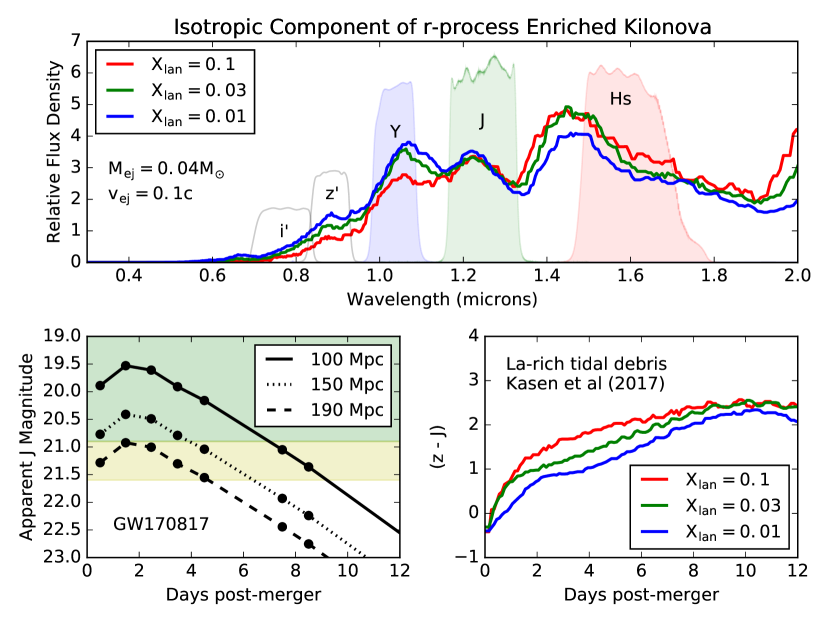
Figure 12: Top: Spectral models of kilonova emission at $t=2$ days post-merger (Kasen et al., 2017). All models have an ejected mass of $0.04M_{\odot}$ at velocity $0.1c$, similar to the favored parameters of GW170817 but with varying lanthanide fractions from 1-10%. All models have been normalized to a common flux in $J$, and filter curves show the bandpass of MKO filters weighted by InGaAs quantum efficiency. Bottom left: Observed $J$-band light curve of GW170817 projected to distances between 100-190 Mpc—the expected horizon for Advanced LIGO(Abbott et al., 2016). The green shaded region corresponds to a 5-minute integration depth, whereas the yellow region corresponds to 10 minutes integration. Bottom Right: Temporal evolution of $(z-J)$ color in the models from the top panel as the EM counterpart fades in the first 2 weeks after merger. Rapid fading together with strong reddning is a characteristic signature of lanthanide-rich merger remnants.

Our demonstration camera would detect the fading counterpart of GW170817 in $J$ using 5-minute survey integrations (green shaded region) at $5\sigma$ significance for a week after merger at 100 Mpc, or 4 days at 150 Mpc, and would just miss a detection in 5 minutes at LIGO’s maximum distance. If 10-minute mapping integrations are used (yellow shaded region), the transient is visible for 9 days at 100 Mpc, and 5 days at 190 Mpc. The $(z-J)$ color of the slow, heavy wind rises steeply with time, exhibiting 1-2 magnitudes of reddning over the first few days following merger (Figure 13, bottom right).

With these plots and the sensitivity curves from Figure 6, we can assess the relative merits of an optical survey in the $i^{\prime}$ or $z^{\prime}$ bands versus an infrared InGaAs camera in $Y$, $J$ or $H$.

For concreteness, we assume a fiducial 1 square degree FoV tiled with InGaAs, consistent with an under-filled focal plane on the 2.5-meter DuPont or SDSS telescopes (which have a $\sim 3.1$ square degree field), although similar scaling arguments can be developed for smaller apertures. If we further assume a 10-minute integration cadence, Figure 6 indicates a $5\sigma$ depth of $J_{AB}=21.5-21.7$. At this speed, one could map $\sim 6$ square degrees per hour with sufficient sensitivity to detect the EM counterpart of GW170817 at 150 Mpc for 7 days. At the actual distance of 40 Mpc for GW170817, the $r$-process peak would be visible for over two weeks in 10 minute exposures. At the edge of the Advanced LIGO design horizon of 200 Mpc, it would be visible for 5 days.

Simulations suggest that in the era of two GW detectors (i.e. Advanced LIGO O3), roughly half of all BNS mergers will be localized within $150$ square degrees (Chen et al., 2017), and only 10% will have localizations of 50 square degrees or better. However if the positional region of uncertainty is above the horizon for 3-4 hours per night, one may survey 18-24 square degrees per day to $J_{AB}=21.5$. This is sufficient to tile the most well-localized 10% of events in 2 nights, or survey even unfavorable two-detector error contours in four to five nights (during which time the IR transient is still visible throughout the full 190 Mpc volume).

The same simulations find that inclusion of VIRGO (Accadia et al., 2012) detections during O4 will localize $\sim 70$% of events within approximately 5 square degrees. This region could be surveyed with 1-2 hour cadence to the same depth, but would more likely be integrated to $\geq$1-hour exposure depth reaching $J_{AB}=22.5$ or fainter. This would allow IR instruments to identify mergers with lower ejected mass yields or velocities, consistent with prior expectations for BNS mergers (Kasen et al., 2015). It also provides more margin for events that are dust-obscured or inconveniently placed on the sky. The lower cost of InGaAs could enable blind searches for NS-NS merger counterparts directly in the IR, in parallel with similar searches at optical wavelengths.

Because the EM counterpart of GW170817 was discovered in the optical and existing CCD imagers of larger entendue will already be searching for the same counterparts, one must consider whether there is added value in contemporaneous IR searches using smaller apertures and/or fields. Indeed a rapidly fading optical transient was the first and brightest signal seen from this event on the ground.

There are three possible motivations for pairing deep optical searches with wide-field IR mapping (as opposed to post-discovery followup). First, the radioactively heated IR transient is widely believed to be isotropic, while the angular dependence of the UV-optical radiation is unconstrained at present. An accounting of the fractional contribution of UV-optical transients to the parent population of IR-trggered events will define the geometry and uniformity of the EM mechanisms.

Second, a generic signature of heated-cocoon models is a rapid optical transient that fades by over 1 magnitude per day, concomitant with a rise in the $J$ and $H$ bands over similar time scales—in other words, all bands bluer than $J$ fade continuously. Cowperthwaite et al. (2017a) demonstrated that optical searches can map regions of $\sim 50$ square degrees to $i^{\prime}=22.5$, sufficient to detect a rapid UV-optical transient similar to GW170817 for 3-4 days. Optical searches would not detect emission from the isotropic $r$-process material; they require favorably oriented jets, cocoons, or disk winds to successfully identify EM counterparts.

However Cowperthwaite et al. (2017a) also find that the optical searches exhibit a false-positive rate of $\sim 2$ unrelated transients per square degree in their blind search; after applying priors on color this rate is reduced to $\sim 1$ degree^-2 if kilonovae are assumed to be intrisically blue, or $\sim 0.15$ deg^-2 if they are intrisically red as in $r$-process events. A blind search of $\sim 50$ square degrees would therefore yield between 7 and 100 contaminants depending on priors applied. Early-time monitoring in the $J$ or $H$ bands could establish the simultaneous IR brightening and sustained luminosity unique to NS-NS binary mergers, separating BNS events from unrelated foregrounds.

Third, the long duration of EM signals in the infrared offers an extended window over which to monitor events, in contrast to high-etendue optical campaigns which cannot always encumber the resources of large telescopes for followup on timescales of weeks.

It is projected that aLIGO and VIRGO may discover NS binaries at a rate of 1/month at design sensitivity, such that followup of these events consumes a substantial portion, but not all of small observtories’ time allocations. During times when targeted followups are not underway, such a survey instrument could perform a dedicated wide-field time-domain survey in the IR, a program which has not been undertaken to date largely on account of sensor costs.

7 Conclusions

We report a series of tests from a prototype InGaAs camera deployed on the 2.5-meter DuPont telescope. On an aperture of this size we find that the AP1121 can deliver sky-photon limited noise performance in the $J$ band with $0.4\arcsec$ pixels, and has roughly equal contributions from sky and dark current in $Y$, in operating conditions at $T=-40$C with no cold stop. A modest engineering effort was needed to reduce read noise through non-destructive sampling (not generally available on commercial cameras), to levels where it is quickly exceeded by shot noise from the sky. This indicates that for broadband imaging applications not requiring the $K$ band, InGaAs can be competetive with HgCdTe at substantially reduced cost.

On a 2.5-meter telescope, we measure photometric zero points of $24.5-25.3$ magnitudes in the $Y$ and $J$ bands, demosntrating sufficient sensitivity to image transient sources in the local universe, the red sequence of a $z=0.87$ galaxy cluster, and a $z=6.3$ QSO, typical of static-sky survey targets.

While these devices have less astronomy heritage, their cost savings could make them attractive for wide-field survey instruments on medium sized apertures, or alternatively as low-cost IR photometers on 1-meter apertures with pixels of $\sim 1$″ or larger.

References

- Abbott et al. (2016) Abbott, B. P., et al. 2016, Living Reviews in Relativity, 19, 1
- Abbott et al. (2017) Abbott, B. P., et al. 2017, Phys. Rev. Lett., 119, 161101
- Accadia et al. (2012) Accadia, T., et al. 2012, Journal of Instrumentation, 7, P03012
- Barnes et al. (2016) Barnes, J., Kasen, D., Wu, M.-R., & Martínez-Pinedo, G. 2016, ApJ, 829, 110
- Beletic et al. (2008) Beletic, J. W., et al. 2008, in Proc. SPIE, Vol. 7021, High Energy, Optical, and Infrared Detectors for Astronomy III, 70210H
- Bellm & Kulkarni (2017) Bellm, E., & Kulkarni, S. 2017, Nature Astronomy, 1, 0071
- Benford et al. (2008) Benford, D. J., Lauer, T. R., & Mott, D. B. 2008, in Proc. SPIE, Vol. 7021, High Energy, Optical, and Infrared Detectors for Astronomy III, 70211V
- Bersten et al. (2018) Bersten, M. C., et al. 2018, Nature, 554, 497
- Bertin & Arnouts (1996) Bertin, E., & Arnouts, S. 1996, A&AS, 117, 393
- Carnall et al. (2015) Carnall, A. C., et al. 2015, MNRAS, 451, L16
- Chapman et al. (1990) Chapman, R., Beard, S., Mountain, M., Pettie, D., & Pickup, A. 1990, in Proc. SPIE, Vol. 1235, Instrumentation in Astronomy VII, ed. D. L. Crawford, 34–42
- Chen et al. (2017) Chen, H.-Y., Essick, R., Vitale, S., Holz, D. E., & Katsavounidis, E. 2017, ApJ, 835, 31
- Cowperthwaite et al. (2017a) Cowperthwaite, P. S., et al. 2017a, ArXiv e-prints
- Cowperthwaite et al. (2017b) —. 2017b, ApJ, 848, L17
- de Val-Borro et al. (2016) de Val-Borro, M., et al. 2016, AJ, 152, 161
- Drout et al. (2017) Drout, M. R., et al. 2017, ArXiv e-prints
- Fowler & Gatley (1990) Fowler, A. M., & Gatley, I. 1990, ApJ, 353, L33
- Goobar et al. (2017) Goobar, A., et al. 2017, Science, 356, 291
- Kasen et al. (2013) Kasen, D., Badnell, N. R., & Barnes, J. 2013, ApJ, 774, 25
- Kasen et al. (2015) Kasen, D., Fernández, R., & Metzger, B. D. 2015, MNRAS, 450, 1777
- Kasen et al. (2017) Kasen, D., Metzger, B., Barnes, J., Quataert, E., & Ramirez-Ruiz, E. 2017, ArXiv e-prints
- Kasliwal et al. (2017) Kasliwal, M. M., et al. 2017, ArXiv e-prints
- Law et al. (2009) Law, N. M., et al. 2009, PASP, 121, 1395
- Li & Paczyński (1998) Li, L.-X., & Paczyński, B. 1998, ApJ, 507, L59
- LSST Science Collaboration et al. (2009) LSST Science Collaboration et al. 2009, ArXiv e-prints
- Margutti et al. (2017) Margutti, R., et al. 2017, ApJ, 848, L20
- Menanteau et al. (2012) Menanteau, F., et al. 2012, ApJ, 748, 7
- Metzger & Fernández (2014) Metzger, B. D., & Fernández, R. 2014, MNRAS, 441, 3444
- Metzger et al. (2010) Metzger, B. D., et al. 2010, MNRAS, 406, 2650
- Mooley et al. (2018) Mooley, K. P., et al. 2018, Nature, 554, 207
- Nakar & Sari (2012) Nakar, E., & Sari, R. 2012, ApJ, 747, 88
- Pál (2012) Pál, A. 2012, MNRAS, 421, 1825
- Persson et al. (2013) Persson, S. E., et al. 2013, PASP, 125, 654
- Piro & Kollmeier (2017) Piro, A. L., & Kollmeier, J. A. 2017, ArXiv e-prints
- Skrutskie et al. (2006) Skrutskie, M. F., et al. 2006, AJ, 131, 1163
- Sullivan (2015) Sullivan, P. W. 2015, Master’s thesis, MIT, Cambridge, MA 02139
- Sullivan et al. (2013) Sullivan, P. W., Croll, B., & Simcoe, R. A. 2013, PASP, 125, 1021
- Sullivan et al. (2014) Sullivan, P. W., Croll, B., & Simcoe, R. A. 2014, in Proc. SPIE, Vol. 9154, High Energy, Optical, and Infrared Detectors for Astronomy VI, 91541F
- Tokunaga et al. (2002) Tokunaga, A. T., Simons, D. A., & Vacca, W. D. 2002, PASP, 114, 180
- Villar et al. (2017) Villar, V. A., et al. 2017, ApJ, 851, L21