Minimum-gain Pole Placement with Sparse Static Feedback

Abstract

The minimum-gain eigenvalue assignment/pole placement problem (MGEAP) is a classical problem in LTI systems with static state feedback. In this paper, we study the MGEAP when the state feedback has arbitrary sparsity constraints. We formulate the sparse MGEAP problem as an equality-constrained optimization problem and present an analytical characterization of its locally optimal solution in terms of eigenvector matrices of the closed loop system. This result is used to provide a geometric interpretation of the solution of the non-sparse MGEAP, thereby providing additional insights for this classical problem. Further, we develop an iterative projected gradient descent algorithm to obtain local solutions for the sparse MGEAP using a parametrization based on the Sylvester equation. We present a heuristic algorithm to compute the projections, which also provides a novel method to solve the sparse EAP. Also, a relaxed version of the sparse MGEAP is presented and an algorithm is developed to obtain approximately sparse local solutions to the MGEAP. Finally, numerical studies are presented to compare the properties of the algorithms, which suggest that the proposed projection algorithm converges in most cases.

I Introduction

The Eigenvalue/Pole Assignment Problem (EAP) using static state feedback is one of the central problems in the design of Linear Time Invariant (LTI) control systems (e.g., see [1, 2]). It plays a key role in system stabilization and shaping its transient behavior. Given the following LTI system

$$\mathcal{D}x(k) =Ax(k)+Bu(k),$$ (1a)

$$u(k) =Fx(k),$$ (1b)

where $x\in\mathbb{R}^{n}$ is the state of the LTI system, $u\in\mathbb{R}^{m}$ is the control input, $A\in\mathbb{R}^{n\times n}$, $B\in\mathbb{R}^{n\times m}$, and $\mathcal{D}$ denotes either the continuous time differential operator or the discrete-time shift operator, the EAP involves finding a real feedback matrix $F\in\mathbb{R}^{m\times n}$ such that the eigenvalues of the closed loop matrix $A_{c}(F)\triangleq A+BF$ coincide with a given set $\mathcal{S}=\{\lambda_{1},\lambda_{2},\cdots,\lambda_{n}\}$ that is closed under complex conjugation.

It is well known that the existence of $F$ depends on the controllability properties of the pair $(A,B)$. Further, for single input systems ($m=1$), the feedback vector that assigns the eigenvalues is unique and can be obtained using the Ackermann’s formula [3]. On the other hand, for multi-input systems ($m>1$), the feedback matrix is not unique and there exists a flexibility to choose the eigenvectors of the closed loop system. This flexibility can be utilized to choose a feedback matrix that satisfies some auxiliary control criteria in addition to assigning the eigenvalues. For instance, the feedback matrix can be chosen to minimize the sensitivity of the closed loop system to perturbations in the system parameters, thereby making the system robust. This is known as Robust Eigenvalue Assignment Problem (REAP) [4]. Alternatively, one can choose the feedback matrix with minimum gain, thereby reducing the overall control effort. This is known as Minimum Gain Eigenvalue Assignment Problem (MGEAP) [5, 6].

Recently, considerable attention has been given to the study and design of sparse feedback control systems, where certain entries of the matrix $F$ are required to be zero. Feedback sparsity typically arises in decentralized control problems for large scale and interconnected systems with multiple controllers [7], where each controller has access to only some partial states of the system. Such constraints in decentralized control problems are typically specified by information patterns that govern which controllers have access to which states of the system [8, 9]. Sparsity may also be a result of the special structure of a centralized control system which prohibits feedback from some states to the controllers.

The feedback design problem with sparsity constraints is considerably more difficult than the unconstrained case. There have been numerous studies to determine the optimal feedback control law for H2/LQR/LQG control problems with sparsity, particularly when the controllers have access to only local information (see [8, 7, 10, 9] and the references therein). While the optimal H2/LQR/LQG design problems with sparsity have a rich history, studies on the REAP/MGEAP in the presence of arbitrary sparsity constraints are lacking. Even the problem of finding a particular (not necessary optimal) sparse feedback matrix that solves the EAP is not well studied. In this paper, we study the EAP and MGEAP with arbitrary sparsity constraints on the feedback matrix $F$. We provide analytical characterization for the solution of sparse MGEAP and provide iterative algorithms to solve the sparse EAP and MGEAP. We also briefly discuss the feasibility of the sparse EAP problem.

Related work There have been numerous studies on the optimal pole placement problem without sparsity constraints. For the REAP, authors have considered optimizing different metrics which capture the sensitivity of the eigenvalues, such as the condition number of the eigenvector matrix [4, 11, 12, 13, 14], departure from normality [15] and others [16, 17]. Most of these methods use gradient-based iterative procedures to obtain the solutions. For surveys and comparisons of these REAP methods, see [11, 18, 19] and the references therein.

Early works for MGEAP, including [20, 21], presented approximate solutions using low rank feedback and successive pole placement techniques. Simultaneous robust and minimum gain pole placement were studied in [22, 14, 23, 24]. For a survey and performance comparison of these MGEAP studies, see [5] and the references therein. The regional pole placement problem was studied in [25], [26], where the eigenvalues were assigned inside a specified region. While these studies have provided useful insights on REAP/MGEAP, they do not consider sparsity constraints on the feedback matrix. In contrast, we study the sparse EAP/MGEAP by explicitly including the sparsity constraints in the problem formulation and solutions.

There have also been numerous studies on EAP with sparse dynamic LTI feedback. The concept of decentralized fixed modes (DFMs) was introduced in [27] and later refined in [28]. Decentralized fixed modes are those eigenvalues of the system which cannot be shifted using a static/dynamic feedback with fully decentralized sparsity pattern (i.e. the case where controllers have access only to local states). The remaining eigenvalues of the system can be arbitrarily assigned. However, this cannot be achieved in general using a static decentralized controller and requires the use of dynamic decentralized controller [27]. Other algebraic characterizations of the DFMs were presented in [29, 30]. The notion of DFMs was generalized for an arbitrary sparsity pattern and the concept of structurally fixed modes (SFMs) was introduced in [31]. Graph theoretical characterizations of structurally fixed modes were provided in [32, 33]. As in the case of DFMs, assigning the non-SFMs also requires dynamic controllers. These studies on DFMs and SFMs present feasibility conditions and analysis methods for the EAP problem with sparse dynamic feedback. In contrast, we study both EAP and MGEAP with sparse static controllers, assuming the sparse EAP is feasible. We remark that EAP with sparsity and static feedback controller is in fact important for several network design and control problems, and easier to implement than its dynamic counterpart.

Recently, there has been a renewed interest in studying linear systems with sparsity constraints. Using a different approach than [32], the original results regarding DFMs in [27] were generalized for an arbitrary sparsity pattern by the authors in [34, 35], where they also present a sparse dynamic controller synthesis algorithm. Further, there have been many recent studies on minimum cost input/output and feedback sparsity pattern selection such that the system has controllability [36] and no structurally fixed modes (see [37, 38] and the references therein). In contrast, we consider the problem of finding a static minimum gain feedback with a given sparsity pattern that solves the EAP.

Contribution The contribution of this paper is three-fold. First, we study the MGEAP with static feedback and arbitrary sparsity constraints (assuming feasibility of sparse EAP). We formulate the sparse MGEAP as an equality constrained optimization problem and present an analytical characterization of an locally optimal sparse solution. As a minor contribution, we use this result to provide a geometric insight for the non-sparse MGEAP solutions. Second, we show that determining the feasibility of the sparse EAP is NP-hard and present necessary and sufficient conditions for feasibility. We develop two heuristic iterative algorithms to obtain a local solution of the sparse EAP. The first algorithm is based on repeated projections on linear subspaces. The second algorithm is developed using the Sylvester equation based parametrization and it obtains a solution via projection of a non-sparse feedback matrix on the space of sparse feedback matrices that solve the EAP. Third, using the latter EAP projection algorithm, we develop a projected gradient descent method to obtain a local solution to the sparse MGEAP. We also formulate a relaxed version of the sparse MGEAP using penalty based optimization and develop an algorithm to obtain approximately-sparse local solutions.

Paper organization The remainder of the paper is organized as follows. In Section II we formulate the sparse MGEAP optimization problem. In Section III, we obtain the solution of the optimization problem using the Lagrangian theory of optimization. We also provide a geometric interpretation for the optimal solutions of the non-sparse MGEAP. In Section IV, we present two heuristic algorithms for solving the sparse EAP. Further, we present a projected gradient descent algorithm to solve the sparse MGEAP and also an approximately-sparse solution algorithm for a relaxed version of the sparse MGEAP. Section V contains numerical studies and comparisons of the proposed algorithms. In Section VI, we discuss the feasibility of the sparse EAP. Finally, Section VII concludes the paper.

II Sparse MGEAP formulation

II-A Mathematical notation and preliminary properties

We use the following properties to derive our results [39, 40]:

1. $\text{tr}(A)=\text{tr}(A^{\mathsf{T}})\>\text{ and }\>\text{tr}(ABC)=\text{tr}(CAB)$,

2. $\|A\|_{\text{F}}^{2}=\text{tr}(A^{\mathsf{T}}A)=\text{vec}^{\mathsf{T}}(A)\text{vec}(A)$,

3. $\text{vec}(AB)=(I\otimes A)\text{vec}(B)=(B^{\mathsf{T}}\otimes I)\text{vec}(A)$,

4. $\text{vec}(ABC)=(C^{\mathsf{T}}\otimes A)\text{vec}(B)$,

5. $(A\otimes B)^{\mathsf{T}}=A^{\mathsf{T}}\otimes B^{\mathsf{T}}$ and $(A\otimes B)^{\mathsf{H}}=A^{\mathsf{H}}\otimes B^{\mathsf{H}}$,

6. $1_{n}^{\mathsf{T}}(A\circ B)1_{n}=\text{tr}(A^{\mathsf{T}}B)$,

7. $A\circ B=B\circ A\>\text{ and }\>A\circ(B\circ C)=(A\circ B)\circ C$,

8. $\text{vec}(A\circ B)=\text{vec}(A)\circ\text{vec}(B),(A\circ B)^{\mathsf{T}}=A^{\mathsf{T}}\circ B^{\mathsf{T}}$,

9. $\frac{d}{dX}\text{tr}(AX)\!=\!A^{\mathsf{T}}$, $\frac{d}{dX}\text{tr}(X^{\mathsf{T}}X)\!=\!2X$, $\frac{d}{dx}(Ax)\!=\!A$,

10. $d(X^{-1})=-X^{-1}dXX^{-1}$,

11. Let $D_{x}f$ and $D^{2}_{x}f$ be the gradient and Hessian of
        $f(x):\mathbb{R}^{n}\rightarrow\mathbb{R}$. Then, $df=(D_{x}f)^{\mathsf{T}}dx$ and
        $d^{2}f=(dx)^{\mathsf{T}}(D^{2}_{x}f)dx$,

12. Projection of a vector $y\in\mathbb{R}^{n}$ on the null space of      $A\in\mathbb{R}^{m\times n}$ is given by $y_{p}=[I_{n}-A^{+}A]y$.

The Kronecker sum of two square matrices $A$ and $B$ with dimensions $n$ amd $m$, respectively, is denoted by

$$A\oplus B=(I_{m}\otimes A)+B\otimes I_{n}.$$

Further, we use the following notation throughout the paper:

$\|\cdot\|_{2}$	Spectral norm
$\|\cdot\|_{\text{F}}$	Frobenius norm
$<\cdot,\cdot>_{F}$	Inner (Frobenius) product
$\lvert\cdot\rvert$	Cardinality of a set
$\Gamma(\cdot)$	Spectrum of a matrix
$\sigma_{min}(\cdot)$	Minimum singular value of a matrix
$\text{tr}(\cdot)$	Trace of a matrix
$(\cdot)^{+}$	Moore-Penrose pseudo inverse
$(\cdot)^{\mathsf{T}}$	Transpose of a matrix
$\mathcal{R}(\cdot)$	Range of a matrix
$A>0$	Positive definite matrix $A$
$\circ$	Hadamard (element-wise) product
$\otimes$	Kronecker product
$(\cdot)^{*}$	Complex conjugate
$(\cdot)^{\mathsf{H}}$	Conjugate transpose
$\text{supp}(\cdot)$	Support of a vector
$\text{vec}(\cdot)$	Vectorization of a matrix
$\text{diag}(a)$	$n\times n$ Diagonal matrix with diagonal
	elements given by $n$-dim vector $a$
$\text{Re}(\cdot)$	Real part of a complex variable
$\text{Im}(\cdot)$	Imaginary part of a complex variable
$1_{n}(0_{n})$	$n$-dim vector of ones (zeros)
$1_{n\times m}(0_{n\times m})$	$n\times m$-dim matrix of ones (zeros)
$I_{n}$	$n$-dim identity matrix
$e_{i}$	$i$-th canonical vector
$T_{m,n}$	Permutation matrix that satisfies
	$\text{vec}(A^{\mathsf{T}})=T_{m,n}\text{vec}(A)$, $A\in\mathbb{R}^{m\times n}$

II-B Sparse MGEAP

The sparse MGEAP involves finding a real feedback matrix $F\in\mathbb{R}^{m\times n}$ with minimum norm that assigns the closed loop eigenvalues of (1a)-(1b) at some desired locations given by set $\mathcal{S}=\{\lambda_{1},\lambda_{2},\cdots,\lambda_{n}\}$, and satisfies a given sparsity constraints. Let $\bar{\mathsf{F}}\in\{0,1\}^{m\times n}$ denote a binary matrix that specifies the sparsity structure of the feedback matrix $F$. If $\bar{\mathsf{F}}_{ij}=0$ (respectively $\bar{\mathsf{F}}_{ij}=1$), then the $j^{\text{th}}$ state is unavailable (respectively available) for calculating the $i^{\text{th}}$ input. Thus,

$$F_{ij}=\begin{cases}0\quad\text{if}\>\>\bar{\mathsf{F}}_{ij}=0,\>\>\text{and}\\ \star\quad\text{if}\>\>\bar{\mathsf{F}}_{ij}=1,\end{cases}$$

where $\star$ denotes a real number. Let $\bar{\mathsf{F}}^{c}\triangleq 1_{m\times n}-\bar{\mathsf{F}}$ denote the complementary sparsity structure matrix. Further, (with a slight abuse of notation, c.f. (1a)) let $X\triangleq[x_{1},x_{2},\cdots,x_{n}]\in\mathbb{C}^{n\times n},x_{i}\neq 0_{n}$ denote the non-singular eigenvector matrix of the closed loop matrix $A_{c}(F)=A+BF$.

The MGEAP can be mathematically stated as follows:

$$\underset{F,X}{\min} \quad\frac{1}{2}\>||F||_{F}^{2}\hskip 110.0pt$$ (2)

s.t. $$\quad(A+BF)X=X\Lambda,$$ (2a)

$$\quad\bar{\mathsf{F}}^{c}\circ F=0_{m\times n},$$ (2b)

where $\Lambda=\text{diag}([\lambda_{1},\lambda_{2},\cdots,\lambda_{n}]^{\mathsf{T}})$ is the diagonal matrix of the desired eigenvalues. Equations (2a) and (2b) represent the eigenvalue assignment and sparsity constraints, respectively.

The constraint (2a) is not convex in $(F,X)$ and, therefore, the optimization problem (2) is non-convex. Consequently, multiple local minima may exist. This is a common feature in various minimum distance and eigenvalue assignment problems [41], including the non-sparse MGEAP.

Remark 1.

(Choice of norm) The Frobenius norm measures the element-wise gains of a matrix, which is informative in sparsity constrained problems arising, for instance, in network control problems. It is also convenient for the analysis, particularly to compute the derivatives of the cost function. $\square$

Definition 1.

(Fixed modes [34, 27]) The fixed modes of $(A,B)$ with respect to the sparsity constraints $\bar{\mathsf{F}}$ are those eigenvalues of $A$ which cannot be changed using LTI static (and also dynamic) state feedback, and are denoted by

$$\Gamma_{f}(A,B,\bar{\mathsf{F}})\triangleq\underset{\textstyle F:F\circ\bar{\mathsf{F}}^{c}=0}{\bigcap}\Gamma(A+BF).$$

We make the following assumptions regarding the fixed modes and feasibility of the optimization problem (2).

Assumption 1.

The fixed modes of the triplet $(A,B,\bar{\mathsf{F}})$ are included in the desired eigenvalue set $\mathcal{S}$, i.e., $\Gamma_{f}(A,B,\bar{\mathsf{F}})\subseteq\mathcal{S}$.

Assumption 2.

There exists at least one feedback matrix $F$ that satisfies constraints (2a)-(2b) for the given $\mathcal{S}$.

Assumption 1 is clearly necessary for the feasibility of the optimization problem (2). Assumption 2 is restrictive because, in general, it is possible that a static feedback matrix with a given sparsity pattern cannot assign the closed loop eigenvalues to arbitrary locations (i.e. for an arbitrary set $\mathcal{S}$ satisfying Assumption 1). In such cases, only a few ($<n$) eigenvalues can be assigned independently and other remaining eigenvalues are a function of them. To the best of our knowledge, there are no studies on characterizing conditions for the existence of a static feedback matrix for an arbitrary sparsity pattern $\bar{\mathsf{F}}$ and eigenvalue set $\mathcal{S}$ [42] (although such characterization is available for dynamic feedback laws with arbitrary sparsity pattern [31, 34, 35], and static output feedback for decentralized sparsity pattern [43]). Thus, for the purpose of this paper, we focus on finding the optimal feedback matrix assuming that at least one such feedback matrix exists. We provide some preliminary results on the feasibility of the optimization problem (2) in Section VI.

III Solution to the sparse MGEAP

In this section we present the solution to the optimization problem (2). To this aim, we use the theory of Lagrangian multipliers for equality constrained minimization problems.

Remark 2.

(Conjugate eigenvectors) We use the convention that the right (respectively, left) eigenvectors $(x_{i},x_{j})$ corresponding to two conjugate eigenvalues $(\lambda_{i},\lambda_{j})$ are also conjugate. Thus, if $\lambda_{i}=\lambda_{j}^{*}$, then $x_{i}=x_{j}^{*}$. $\square$

We use the real counterpart of (2a) for the analysis. For two complex conjugate eigenvalues $(\lambda_{i},\lambda_{i}^{*})$ and corresponding eigenvectors $(x_{i},x_{i}^{*})$, the following complex equation

$$(A+BF)\begin{bmatrix}x_{i}&x_{i}^{*}\end{bmatrix}=\begin{bmatrix}x_{i}&x_{i}^{*}\end{bmatrix}\left[\begin{smallmatrix}\lambda_{i}&0\\ 0&\lambda_{i}^{*}\end{smallmatrix}\right]$$

is equivalent to the following real equation

$$(A\!+\!BF)\!\begin{bmatrix}\text{Re}(x_{i})&\text{Im}(x_{i})\end{bmatrix}\!\!=\!\!\begin{bmatrix}\text{Re}(x_{i})&\text{Im}(x_{i})\end{bmatrix}\!\!\left[\begin{smallmatrix}\phantom{-}\text{Re}(\lambda_{i})&\text{Im}(\lambda_{i})\\ -\text{Im}(\lambda_{i})&\text{Re}(\lambda_{i})\end{smallmatrix}\right].$$

For each complex eigenvalue, the columns $\begin{bmatrix}x_{i}&x_{i}^{*}\end{bmatrix}$ of $X$ are replaced by $\begin{bmatrix}\text{Re}(x_{i})&\text{Im}(x_{i})\end{bmatrix}$ to obtain a real $X_{R}$, and the sub-matrix $\left[\begin{smallmatrix}\lambda_{i}&0\\ 0&\lambda_{i}^{*}\end{smallmatrix}\right]$ of $\Lambda$ is replaced by $\left[\begin{smallmatrix}\phantom{-}\text{Re}(\lambda_{i})&\text{Im}(\lambda_{i})\\ -\text{Im}(\lambda_{i})&\text{Re}(\lambda_{i})\end{smallmatrix}\right]$ to obtain a real $\Lambda_{R}$. The real eigenvectors in $X$ and $X_{R}$, and real eigenvalues in $\Lambda$ and $\Lambda_{R}$ coincide. Clearly, $X_{R}$ is not the eigenvector matrix of $A+BF$ (c.f. Remark 7), and $X$ can be obtained through the columns of $X_{R}$. Thus, (2a) becomes

$$(A+BF)X_{R}=X_{R}\Lambda_{R},$$ (3)

and $X_{R}$ replaces the optimization variable $X$ in (2). In the theory of equality constrained optimization, the first-order optimality conditions are meaningful only when the optimal point satisfies the following regularity condition: the Jacobian of the constraints, defined by $J_{b}$, is full rank. This regularity condition is mild and usually satisfied for most classes of problems [44]. Before presenting the main result, we derive the Jacobian and state the regularity condition for the problem (2).

Computation of $J_{b}$ requires vectorization of the matrix constraints (3) and (2b). For this purpose, let $x_{R}\triangleq\text{vec}(X_{R})\in\mathbb{C}^{n^{2}}$, $f\triangleq\text{vec}(F)\in\mathbb{R}^{mn}$, and let $z\triangleq[x_{R}^{\mathsf{T}},f^{\mathsf{T}}]^{\mathsf{T}}$ be the vector containing all the independent variables of the optimization problem. Further, let $n_{s}$ denote the total number of feedback sparsity constraints (i.e. number of $1$’s in $\bar{\mathsf{F}}^{c}$):

$${n}_{\textup{s}} =|\{(i,j)\;:\;\bar{\mathsf{F}}^{c}=[\bar{\mathsf{f}}^{c}_{ij}],\,\bar{\mathsf{f}}^{c}_{ij}=1\}|.$$

Note that the constraint (2b) consists of $n_{s}$ non-trivial sparsity constraints, and can be equivalently written as

$$Qf=0_{n_{s}},$$ (4)

where $Q=\begin{bmatrix}e_{q_{1}}&e_{q_{2}}&\dots&e_{q_{n_{s}}}\end{bmatrix}^{\mathsf{T}}\in\{0,1\}^{n_{s}\times mn}$ with $\{q_{1},\dots,q_{n_{s}}\}=\text{supp}(\text{vec}(\bar{\mathsf{F}}^{c}))$ being the set of indices indicating the ones in $\text{vec}(\bar{\mathsf{F}}^{c})$.

Lemma 3.

(Jacobian of the constraints) The Jacobian of the equality constraints (2a)-(2b) is given by

$$J_{b}(z)=\begin{bmatrix}{A}_{c}(F)\!\oplus\!(\!-\Lambda_{R}^{\mathsf{T}})&X_{R}^{\mathsf{T}}\!\otimes\!B\\ 0_{n_{s}\times n^{2}}&Q\end{bmatrix}.$$ (5)

Proof.

We construct the Jacobian $J_{b}$ by rewriting the constraints (3) and (2b), in vectorized form and taking their derivatives with respect to $z$. Constraint (3) can be vectorized in the following two different ways (using P.3 and P.4):

$$[(A+BF)\oplus(-\Lambda_{R}^{\mathsf{T}})]x_{R}=0_{n^{2}},$$ (6a)

$$[A\oplus-(\Lambda_{R}^{\mathsf{T}})]x_{R}+(X_{R}^{\mathsf{T}}\otimes B)f=0_{n^{2}}.$$ (6b)

Differentiating (6a) w.r.t. $x_{R}$ and (6b) w.r.t $f$ yields the first (block) row of $J_{b}$. Differentiating (4) w.r.t. $z$ yields the second (block) row of $J_{b}$, thus completing the proof. ∎

We now state the optimality conditions for the problem (2).

Theorem 4.

(Optimality conditions) Let $(\hat{X},\hat{F})$ (equivalently $\hat{z}=[\hat{x}_{R}^{\mathsf{T}},\hat{f}^{\mathsf{T}}]^{\mathsf{T}}$) satisfy the constraints (2a)-(2b). Let $\hat{L}=[\hat{l}_{i}]$, $i=1,\cdots,n$ be the left eigenvector matrix of $A_{c}(\hat{F})$, and let $\hat{L}_{R}$ be its real counterpart constructed by replacing $[\hat{l}_{i},\hat{l}_{i}^{*}]$ with $[\textup{Re}(\hat{l}_{i}),-\textup{Im}(\hat{l}_{i})]$. Let $J_{b}(z)$ be defined in Lemma 3 and $P(z)=I_{n^{2}+mn}-J_{b}^{+}(z)J_{b}(z)$. Further, define $\bar{L}\triangleq 4T_{n,m}(B^{\mathsf{T}}\hat{L}_{R}\otimes I_{n})$ and let

$$\hat{D}\triangleq\begin{bmatrix}0_{n^{2}\times n^{2}}&\bar{L}^{\mathsf{T}}\\ \bar{L}&2I_{mn}\end{bmatrix}.$$ (7)

Then, $(\hat{X},\hat{F})$ is a local minimum of the optimization problem (2) if and only if

$$\hat{F}=-\bar{\mathsf{F}}\circ(B^{\mathsf{T}}\hat{L}\hat{X}^{\mathsf{T}}),$$ (8a)

$$(A+B\hat{F})\hat{X}=\hat{X}\Lambda$$ (8b)

$$(A+B\hat{F})^{\mathsf{T}}\hat{L}=\hat{L}\Lambda$$ (8c)

$$J_{b}(\hat{z})\>\>\text{is full rank,}$$ (8d)

$$P(\hat{z})\hat{D}P(\hat{z})>0.$$ (8e)

Proof.

We prove the result using the Lagrange theorem for equality constrained minimization. Let $L_{R}\in\mathbb{R}^{n\times n}$ and $M\in\mathbb{R}^{m\times n}$ be the Lagrange multipliers associated with constraints (3) and (2b), respectively. The Lagrange function for the optimization problem (2) is given by

$$\mathcal{L}\overset{\ref{prop:frob}}{=} \frac{1}{2}\>\text{tr}(F^{\mathsf{T}}F)+2\>1_{n}^{\mathsf{T}}[L_{R}\circ(A_{c}(F)X_{R}-X_{R}\Lambda_{R})]1_{n}$$

$$+1_{m}^{\mathsf{T}} [M\circ(\bar{\mathsf{F}}^{c}\circ F)]1_{n}$$

$$\overset{\ref{prop:lag_mult},\ref{prop:had1}}{=} \frac{1}{2}\>\text{tr}(F^{\mathsf{T}}F)+2\>\text{tr}[L_{R}^{\mathsf{T}}(A_{c}(F)X_{R}-X_{R}\Lambda_{R})]$$

$$+ \text{tr}[(M\circ\bar{\mathsf{F}}^{c})^{\mathsf{T}}F].$$

Necessity: We next derive the first-order necessary condition for a stationary point. Differentiating $\mathcal{L}$ w.r.t. $X_{R}$ and setting to $0$, we get

$$\frac{d}{dX_{R}}\mathcal{L}\overset{\ref{prop:der}}{=}2[A_{c}^{\mathsf{T}}(F)L_{R}-L_{R}\Lambda_{R}^{\mathsf{T}}]=0_{n\times n}.$$ (9)

The real equation (9) is equivalent to the complex equation (8c). Equation (8b) is a restatement of (2a) for the optimal $(\hat{F},\hat{X})$. Differentiating $\mathcal{L}$ w.r.t. $F$, we get

$$\frac{d}{dF}\mathcal{L}\overset{\ref{prop:der}}{=}F+2B^{\mathsf{T}}L_{R}X_{R}^{\mathsf{T}}+M\circ\bar{\mathsf{F}}^{c}=0_{m\times n}.$$ (10)

Taking the Hadamard product of (10) with $\bar{\mathsf{F}}^{c}$ and using (2b), we get (since $\bar{\mathsf{F}}^{c}\circ\bar{\mathsf{F}}^{c}=\bar{\mathsf{F}}^{c}$)

$$\bar{\mathsf{F}}^{c}\circ(2B^{\mathsf{T}}L_{R}X_{R}^{\mathsf{T}})+M\circ\bar{\mathsf{F}}^{c}=0_{m\times n}$$ (11)

Replacing $M\circ\bar{\mathsf{F}}^{c}$ from (11) into (10), we get

$$F=-\bar{\mathsf{F}}\circ(2B^{\mathsf{T}}L_{R}X_{R}^{\mathsf{T}})\overset{(a)}{=}-\bar{\mathsf{F}}\circ(B^{\mathsf{T}}LX^{\mathsf{T}}),$$

where $(a)$ follows from the definition of $L_{R}$ and $X_{R}$ and Remark 2. Equation (8d) is the necessary regularity condition and follows from Lemma 3

Sufficiency: Next, we derive the second-order sufficient condition for a local minimum by calculating the Hessian of $\mathcal{L}$. Taking the differential of $\mathcal{L}$ twice, we get

$$d^{2}\mathcal{L} =\text{tr}((dF)^{\mathsf{T}}dF)+4\text{tr}(L_{R}^{\mathsf{T}}BdFdX_{R})$$

$$\overset{(\ref{prop:frob})}{=}df^{\mathsf{T}}df+4\text{vec}^{\mathsf{T}}(dF^{\mathsf{T}}B^{\mathsf{T}}L_{R})dx_{R}$$

$$\overset{(\ref{prop:vec1},\ref{prop:kron})}{=}df^{\mathsf{T}}df+df^{\mathsf{T}}\bar{L}dx$$

$$=\frac{1}{2}\begin{bmatrix}dx^{\mathsf{T}}&df^{\mathsf{T}}\end{bmatrix}D\begin{bmatrix}dx\\ df\end{bmatrix},$$

where $D$ is the Hessian (c.f. P.11) defined in (7). The sufficient second-order optimality condition for the optimization problem requires the Hessian to be positive definite in the kernel of the Jacobian at the optimal point [44, Chapter 11]. That is, $y^{\mathsf{T}}Dy>0,\;\forall y:J_{b}(z)y=0$. This condition is equivalent to $P(z)DP(z)>0$, since $J_{b}(z)y=0$ if and only if $y=P(z)s$ for a $s\in\mathbb{R}^{n^{2}+mn}$ [44]. Since the projection matrix $P(z)$ is symmetric, (8e) follows, and this concludes the proof. ∎

Observe that the Hadamard product in (8a) guarantees that the feedback matrix satisfies the sparsity constraints given in (2b). However, the optimal sparse feedback $\hat{F}$ cannot be obtained by sparsification of the optimal non-sparse feedback. The optimality condition (8a) is an implicit condition in terms of the closed loop right and left eigenvector matrices. Next, we provide an explicit optimality condition in terms of $\{\hat{L},\hat{X}\}$.

Corollary 5.

(Stationary point of (2)) $\hat{Z}\triangleq[\hat{X}^{\mathsf{T}},\hat{L}^{\mathsf{T}}]^{\mathsf{T}}$ is a stationary point of the optimization problem (2) if and only if

$$\bar{A}\hat{Z}-\hat{Z}\Lambda=\bar{B}_{1}[\mathsf{F}\circ(\bar{B}_{1}^{\mathsf{T}}\bar{I}\hat{Z}\hat{Z}^{\mathsf{T}}\bar{B}_{2})]\bar{B}_{2}^{\mathsf{T}}\hat{Z},$$ (12)

where,

$$\bar{A} \triangleq\begin{bmatrix}A&0_{n\times n}\\ 0_{n\times n}&A^{\mathsf{T}}\end{bmatrix},\>\bar{B}_{1}\triangleq\begin{bmatrix}B&0_{n\times n}\\ 0_{n\times m}&I_{n}\end{bmatrix},$$

$$\bar{B}_{2} \triangleq\begin{bmatrix}I_{n}&0_{n\times m}\\ 0_{n\times n}&B\end{bmatrix},\>\>\mathsf{F}\triangleq\begin{bmatrix}\bar{\mathsf{F}}&0_{m\times m}\\ 0_{n\times n}&\bar{\mathsf{F}}^{\mathsf{T}}\end{bmatrix},\text{and}$$

$$\bar{I} \triangleq\begin{bmatrix}0_{n\times n}&I_{n}\\ I_{n}&0_{n\times n}\end{bmatrix}.$$

Proof.

Combining (8b) and (8c) and using $\Lambda^{\mathsf{T}}=\Lambda$, we get

$$\begin{bmatrix}A\hat{X}-\hat{X}\Lambda\\ A^{\mathsf{T}}\hat{L}-\hat{L}\Lambda\end{bmatrix}=-\begin{bmatrix}B\hat{F}\hat{X}\\ \hat{F}^{\mathsf{T}}B^{\mathsf{T}}\hat{L}\end{bmatrix}$$

$$\Rightarrow\bar{A}\hat{Z}-\hat{Z}\Lambda=-\bar{B}_{1}\begin{bmatrix}\hat{F}&0\\ 0&\hat{F}^{\mathsf{T}}\end{bmatrix}\bar{B}_{2}^{\mathsf{T}}\hat{Z}$$

$$=\bar{B}_{1}\begin{bmatrix}\bar{\mathsf{F}}\circ(B^{\mathsf{T}}\hat{L}\hat{X}^{\mathsf{T}})&0\\ 0&\bar{\mathsf{F}}^{\mathsf{T}}\circ(\hat{X}\hat{L}^{\mathsf{T}}B)\end{bmatrix}\bar{B}_{2}^{\mathsf{T}}\hat{Z}$$

$$=\bar{B}_{1}\left(\mathsf{F}\circ\left\{\bar{B}_{1}^{\mathsf{T}}\begin{bmatrix}\hat{L}\hat{X}^{\mathsf{T}}&0\\ 0&\hat{X}\hat{L}^{\mathsf{T}}\end{bmatrix}\bar{B}_{2}\right\}\right)\bar{B}_{2}^{\mathsf{T}}\hat{Z}$$

$$=\bar{B}_{1}\left(\mathsf{F}\circ\left\{\bar{B}_{1}^{\mathsf{T}}\bar{I}(\hat{Z}\hat{Z}^{\mathsf{T}}\circ\bar{I})\bar{B}_{2}\right\}\right)\bar{B}_{2}^{\mathsf{T}}\hat{Z}$$

$$=\bar{B}_{1}\{\mathsf{F}\circ(\bar{B}_{1}^{\mathsf{T}}\bar{I}\hat{Z}\hat{Z}^{\mathsf{T}}\bar{B}_{2})\}\bar{B}_{2}^{\mathsf{T}}\hat{Z},$$

where the equalities follow from the Hadamard product. ∎

Remark 6.

(Partial spectrum assignment) The results of Theorem 4 and Corollary 5 are also valid when specifying only $p<n$ eigenvalues (the remaining eigenvalues are functionally related to them; see also the discussion below Assumption 2). In this case, $\Lambda\in\mathbb{C}^{p\times p}$, $\hat{X}\in\mathbb{C}^{n\times p}$ and $\hat{L}\in\mathbb{C}^{n\times p}$. While partial assignment may be useful in some applications, in this paper we focus on assigning all the eigenvalues. $\square$

Remark 7.

(General eigenstructure assignment) Although the optimization problem (2) is formulated by considering $\Lambda$ to be diagonal, the result in Theorem 4 is valid for any general $\Lambda$ satisfying $\Gamma(\Lambda)=\mathcal{S}$. For instance, we can choose $\Lambda$ in a Jordan canonical form. However, note that for a general $\Lambda$, $X$ will cease to be an eigenvector matrix. $\square$

A solution of the optimization problem (2) can be obtained by numerically/iteratively solving the matrix equation (12), which resembles a Sylvester type equation with a non-linear right side, and using (8a) to compute the feedback matrix. The regularity and local minimum of the solution can be verified using (8d) and (8e), respectively. Since the optimization problem is not convex, only local minima can be obtained via this procedure. To improve upon the local solutions, the procedure can be repeated for different initial conditions to solve (12). However, convergence to a global minimum is not guaranteed.

The convergence of the iterative techniques to solve (12) depends substantially on the initial conditions. If they are not chosen properly, convergence may not be guaranteed. Further, the solution of (12) can also represent a local maxima. Therefore, instead of solving (12) directly, we use a different approach based on the gradient descent procedure to obtain a locally minimum solution. Details of this approach and corresponding algorithms are presented in Section IV.

III-A Results for the non-sparse MGEAP

In this subsection, we present some results specific to the case when the optimization problem (2) does not have any sparsity constraints (i.e. $\bar{\mathsf{F}}=1_{m\times n}$). Although the non-sparse MGEAP has been studied previously, these results are novel and further illustrate the properties of an optimal solution.

We begin by presenting a geometric interpretation of the optimality conditions in Theorem 4 with $B=I_{n}$, i.e. all the entries of $A$ can be perturbed independently. In this case, the optimization problem (2) can be written as:

$$\underset{X}{\min} \quad\frac{1}{2}\>||A-X\Lambda X^{-1}||_{F}^{2}.$$ (13)

Since $A$ and $R(X)\triangleq X\Lambda X^{-1}$ are elements (or vectors) of the matrix inner product space with Frobenius norm, a solution of the optimization problem (13) is given by the projection of $A$ on the manifold $\mathcal{M}\triangleq\{R(X):X\text{ is non-singular}\}$. This projection can be obtained by solving the normal equation, which states that the optimal error vector $\hat{F}=A-\hat{X}\Lambda\hat{X}^{-1}$ should be orthogonal to the tangent plane of the manifold $\mathcal{M}$ at the optimal point $\hat{X}$ [45]. The next result shows that the optimality conditions derived in Theorem 4 are in fact the normal equations for the optimization problem (13).

Lemma 8.

(Geometric interpretation) Let $\bar{\mathsf{F}}=1_{m\times n}$ and $B=I_{n}$. Then, Equations (8a)-(8c) are equivalent to the following normal equation:

$$<\hat{F},\mathcal{T}_{\mathcal{M}}(\hat{X})>_{F}=0,$$ (14)

where $\mathcal{T}_{\mathcal{M}}(X)$ denotes the tangent space of $\mathcal{M}$ at $X$.

Proof.

We begin by characterizing the tangent space $\mathcal{T}_{\mathcal{M}}(X)$, which is given by the first order approximation of $R(X)$:

$$R(X+dX) =(X+dX)\Lambda(X+dX)^{-1}$$

$$\overset{(\ref{prop:diff_inv})}{=}R(X)+dX\Lambda X^{-1}-X\Lambda X^{-1}dXX^{-1}$$

$$\hskip 42.0pt+\text{higher order terms}.$$

Thus, the tangent space is given by

$$\mathcal{T}_{\mathcal{M}}(X)=\{Y\Lambda X^{-1}-X\Lambda X^{-1}YX^{-1}:Y\in\mathbb{C}^{n\times n}\}$$

Necessity: Using $\hat{F}$ given by (8a), we get

$$<\hat{F}, \mathcal{T}_{\mathcal{M}}(\hat{X})>=\text{tr}(\hat{F}^{\mathsf{T}}(Y\Lambda\hat{X}^{-1}-\hat{X}\Lambda\hat{X}^{-1}Y\hat{X}^{-1}))$$

$$=-\text{tr}(\hat{X}\hat{L}^{\mathsf{T}}Y\Lambda\hat{X}^{-1})+\text{tr}(\hat{X}\hat{L}^{\mathsf{T}}\hat{X}\Lambda\hat{X}^{-1}Y\hat{X}^{-1})$$

$$\overset{(\ref{prop:trace})}{=} -\text{tr}(\hat{L}^{\mathsf{T}}Y\Lambda)+\text{tr}(\hat{L}^{\mathsf{T}}\hat{X}\Lambda\hat{X}^{-1}Y)$$

$$\overset{(a)}{=} -\text{tr}(\hat{L}^{\mathsf{T}}Y\Lambda)+\text{tr}(\Lambda\hat{L}^{\mathsf{T}}\hat{X}\hat{X}^{-1}Y)\overset{(\ref{prop:trace})}{=}0,$$

where $(a)$ follows from the fact that $\Lambda$ and $\hat{L}^{\mathsf{T}}\hat{X}$ commute.

Sufficiency: From (14), we get

$$\text{tr}(\hat{F}^{\mathsf{T}}(Y\Lambda\hat{X}^{-1}-\hat{X}\Lambda\hat{X}^{-1}Y\hat{X}^{-1}))=0$$

$$\overset{(\ref{prop:trace})}{\Rightarrow}\text{tr}[(\Lambda\hat{X}^{-1}\hat{F}^{\mathsf{T}}-\hat{X}^{-1}\hat{F}^{\mathsf{T}}\hat{X}\Lambda\hat{X}^{-1})Y]=0.$$

Since the above equation is true for all $Y\in\mathbb{C}^{n\times n}$, we get

$$\Lambda\hat{X}^{-1} \hat{F}^{\mathsf{T}}-\hat{X}^{-1}\hat{F}^{\mathsf{T}}\hat{X}\Lambda\hat{X}^{-1}=0_{n\times n}$$

$$\Rightarrow\hat{X}\Lambda\hat{X}^{-1}\hat{F}^{\mathsf{T}}=\hat{F}^{\mathsf{T}}\hat{X}\Lambda\hat{X}^{-1}$$

$$\Rightarrow A_{c}(\hat{F})\hat{F}^{\mathsf{T}}=\hat{F}^{\mathsf{T}}A_{c}(\hat{F}).$$

Thus, $A_{c}(\hat{F})$ and $\hat{F}^{\mathsf{T}}$ commute and have common left and right eigenspaces [46], i.e., $\hat{F}^{\mathsf{T}}=-\hat{X}G\hat{X}^{-1}=-\hat{X}\hat{L}^{\mathsf{T}}$, where $G$ is a diagonal matrix. This completes the proof. ∎

Next, we show the equivalence of the non-sparse MGEAP for two orthogonally similar systems.

Lemma 9.

(Invariance under orthogonal transformation) Let $\bar{\mathsf{F}}=1_{m\times n}$ and $(A_{1},B_{1})$, $(A_{2},B_{2})$ be two orthogonally similar systems such that $A_{2}=PA_{1}P^{-1}$ and $B_{2}=PB_{1}$, with $P$ being an orthogonal matrix. Let optimal solutions of (2) for the two systems be denoted by $(\hat{X}_{1},\hat{L}_{1},\hat{F}_{1})$ and $(\hat{X}_{2},\hat{L}_{2},\hat{F}_{2})$, respectively. Then

$$\begin{split}&\hat{X}_{2}=P\hat{X}_{1},\;\hat{L}_{2}=P\hat{L}_{1},\;\hat{F}_{2}=\hat{F}_{1}P^{\mathsf{T}},\text{ and }\\ &||\hat{F}_{1}||_{F}=||\hat{F}_{2}||_{F}.\end{split}$$ (15)

Proof.

From (8b), we have

$$(A_{2}+B_{2}\hat{F_{2}})\hat{X_{2}}=\hat{X_{2}}\Lambda$$

$$\Rightarrow(PA_{1}P^{-1}+PB_{1}\hat{F_{1}}P^{\mathsf{T}})P\hat{X_{1}}=P\hat{X_{1}}\Lambda$$

$$\Rightarrow(A_{1}+B_{1}\hat{F_{1}})\hat{X_{1}}=\hat{X_{1}}\Lambda.$$

Similar relation can be shown between $\hat{L}_{1}$ and $\hat{L}_{2}$ using (8c). Next, from (8a), we have

$$\hat{F}_{2} =-B_{2}^{\mathsf{T}}\hat{L}_{2}\hat{X}_{2}^{\mathsf{T}}=-B_{1}^{\mathsf{T}}\hat{L}_{1}\hat{X}_{1}^{\mathsf{T}}P^{\mathsf{T}}=\hat{F}_{1}P^{\mathsf{T}}.$$

Finally, $||\hat{F}_{1}||_{F}^{2}=\text{tr}(\hat{F}_{1}^{\mathsf{T}}\hat{F}_{1})\overset{(\ref{prop:trace})}{=}\text{tr}(\hat{F}_{2}^{\mathsf{T}}\hat{F}_{2})=||\hat{F}_{2}||_{F}^{2}$. ∎

Recall from Remark 6 that Theorem 4 is also valid for MGEAP with partial spectrum assignment. Next, we consider the case when only one real eigenvalue needs to assigned for the MGEAP while the remaining eigenvalues are unspecified. In this special case, we can explicitly characterize the global minimum of (2) as shown in the next result.

Corollary 10.

(One real eigenvalue assignment) Let $\bar{\mathsf{F}}=1_{m\times n}$, $\Lambda\in\mathbb{R}$, and $B=I_{n}$. Then, the global minima of the optimization problem (2) is given by $\hat{F}_{gl}=-\sigma_{\text{min}}(A-\Lambda I_{n})uv^{\mathsf{T}}$, where $u$ and $v$ are unit norm left and right singular vectors, respectively, corresponding to $\sigma_{\text{min}}(A-\Lambda I_{n})$. Further, $\|\hat{F}_{gl}\rVert_{F}=\sigma_{\text{min}}(A-\Lambda I_{n})$.

Proof.

Since $\Lambda\in\mathbb{R}$, $\hat{X}\in\mathbb{R}^{n}\triangleq\hat{x}$ with $\|\hat{x}\|_{2}=1$, and $\hat{L}\in\mathbb{R}^{n}\triangleq\hat{l}$. Let $\hat{l}=\beta\hat{\tilde{l}}$ where $\beta\triangleq\lVert\hat{l}\rVert_{2}>0$. Substituting $\hat{F}=-\hat{l}\hat{x}^{\mathsf{T}}$ from (8a) into (8b)-(8c), we get

$$(A-\hat{l}\hat{x}^{\mathsf{T}})\hat{x} =\hat{x}\Lambda\Rightarrow(A-\Lambda I_{n})\hat{x}=\beta\hat{\tilde{l}}\quad\text{and,}$$

$$(A^{\mathsf{T}}-\hat{x}\hat{l}^{\mathsf{T}})\hat{l} =\hat{l}\Lambda\Rightarrow(A-\Lambda I_{n})^{\mathsf{T}}\hat{\tilde{l}}=\beta\hat{x}.$$

The above two equations imply that the unit norm vectors $\hat{x}$ and $\hat{\tilde{l}}$ are left and right singular vectors of $A-\Lambda I_{n}$ associated with the singular value $\beta$. Since $\lVert\hat{F}\rVert_{F}^{2}=\text{tr}(\hat{F}^{\mathsf{T}}\hat{F})=\text{tr}(\hat{x}\hat{l}^{\mathsf{T}}\hat{l}\hat{x}^{\mathsf{T}})=\beta^{2}$, we pick $\beta$ as the minimum singular value of $A-\Lambda I_{n}$, and the proof is complete. ∎

We conclude this subsection by presenting a brief comparison of the non-sparse MGEAP solution with deflation techniques for eigenvalue assignment. For $B=I_{n}$, an alternative method to solve the non-sparse EAP is via the Wielandt deflation technique [47]. Wielandt deflation achieves pole assignment by modifying the matrix $A$ in $n$ steps $A\rightarrow A_{1}\rightarrow A_{2}\rightarrow\cdots\rightarrow A_{n}$. Step $i$ shifts one eigenvalue of $A_{i-1}$ to a desired location $\lambda_{i}$, while keeping the remaining eigenvalues of $A_{i-1}$ fixed. This is achieved by using the feedback $F^{i}_{df}=-(\mu_{i}-\lambda_{i})v_{i}z_{i}^{\mathsf{T}}$, where $\mu_{i}$ and $v_{i}$ are any eigenvalue and right eigenvector pair of $A_{i-1}$, and $z_{i}$ is any vector such that $z_{i}^{\mathsf{T}}v_{i}=1$. Thus, the overall feedback that solves the EAP is given as $F_{df}=\sum_{i=1}^{n}F^{i}_{df}$.

It is interesting to compare the optimal feedback expression in (8a), $\hat{F}=-\sum_{i=1}^{n}\hat{l}_{i}\hat{x}_{i}^{\mathsf{T}}$, with the deflation feedback. Both feedbacks are sum of $n$ matrices, where each matrix has rank $1$. However, the Wielandt deflation has an inherent special structure and a restrictive property that, in each step, all except one eigenvalue remain unchanged. Furthermore, each rank$-1$ term in $\hat{F}$ and $F_{df}$ involves the right/left eigenvectors of the closed and open loop matrix, respectively. Clearly, since $\hat{F}$ is the minimum-gain solution of (2), $||\hat{F}||_{F}\leq||F_{df}||_{F}$.

IV Solution algorithms

In this section, we present an iterative algorithm to obtain a solution to the sparse MGEAP in (2). To develop the algorithm, we first present two algorithms for computing non-sparse and approximately-sparse solutions to the MGEAP, respectively. Next, we present two heuristic algorithms to obtain a sparse solution of the EAP (i.e. any sparse solution, which is not necessarily minimum-gain). Finally, we use these algorithms to develop the algorithm for sparse MGEAP. Note that although our focus is to develop the sparse MGEAP algorithm, the other algorithms presented in this section are novel in themselves to the best of our knowledge.

We make the following assumptions:

Assumption 3.

The triplet $(A,B,\bar{\mathsf{F}})$ has no fixed modes, i.e., $\Gamma_{f}(A,B,\bar{\mathsf{F}})=\emptyset$.

Assumption 4.

The open and closed loop eigenvalue sets are disjoint, i.e., $\Gamma(A)\cap\Gamma(\Lambda)=\emptyset$, and $B$ has full column rank.

Assumption 4 is not restrictive since if there are any common eigenvalues in $A$ and $\Lambda$, we can use a preliminary sparse feedback $F_{p}$ to shift the eigenvalues of $A$ to some other locations such that $\Gamma(A+BF_{p})\cap\Gamma(\Lambda)=\emptyset$. Due to Assumption 3, such a $F_{p}$ always exists. Then, we can solve the modified MGEAP with parameters $(A+BF_{p},B,\Lambda,\bar{\mathsf{F}})$. If $F$ is the sparse solution of this modified problem, then the solution of the original problem is $F_{p}+F$.

To avoid complex domain calculations in the algorithms, we use the real eigenvalue assignment constraint (3). For convenience, we use a slight abuse of notation to denote $X_{R}$ and $\Lambda_{R}$ as $X$ and $\Lambda$, respectively, in this section. Note that the invertibility of $X$ is equivalent to the invertibility of $X_{R}$.

IV-A Algorithms for the non-sparse MGEAP

We now present two iterative algorithms to obtain non-sparse and approximately-sparse solutions to the MGEAP, respectively. To develop the algorithms, we use the Sylvester equation based parametrization [48, 14]. In this parametrization, instead of defining $(F,X)$ as free variables, we define a parameter $G\triangleq FX\in\mathbb{R}^{m\times n}$ as the free variable. With this parametrization, the non-sparse MGEAP is stated as:

$$\underset{G}{\min} \quad J=\frac{1}{2}\>||F||_{F}^{2}\hskip 40.0pt$$ (16)

$$\text{s.t.}\quad AX-X\Lambda+BG =0,$$ (16a)

$$F=GX^{-1}$$ . (16b)

Note that, for any given $G$, we can solve the Sylvester equation (16a) to obtain $X$. Assumption 4 guarantees that (16a) has a unique solution [49]. Further, we can use (16b) to obtain a non-sparse feedback matrix $F$. Thus, (16) is an unconstrained optimization problem in the free parameter $G$.

The Sylvester-based parametrization requires the unique solution $X$ of (16a) to be non-singular, which holds generically if (i) $(A,-BG)$ is controllable and (ii) $(\Lambda,-BG)$ is observable [50]. Since the system has no fixed modes, $(A,B)$ is controllable [27]. This implies that condition (i) holds generically for almost all $G$. Further, since $B$ is of full column rank, condition (ii) is guaranteed if $(\Lambda,-G)$ is observable. These conditions are mild and are satisfied for almost all instances as confirmed in our simulations (see Section V).

The next result provides the gradient and Hessian of the cost $J$ w.r.t. to the parameter $g\triangleq\text{vec}(G)$.

Lemma 11.

(Gradient and Hessian of $\mathbf{J})$ The gradient and Hessian of the cost $J$ in (16) with respect to $g$ is given by

$$\frac{dJ}{dg}\!= \!\underbrace{\left[(X^{-1}\!\otimes I_{m})\!+\!(I_{n}\!\otimes B^{\mathsf{T}})\tilde{A}^{-\mathsf{T}}(X^{-1}\!\otimes F^{\mathsf{T}})\right]}_{\textstyle\triangleq Z(F,X)}f,$$ (17)

$$\frac{d^{2}J}{d^{2}g} \triangleq H(F,X)=Z(F,X)Z^{\mathsf{T}}\!(F,X)$$

$$+Z_{1}(F,X)Z^{\mathsf{T}}(F,X)+Z(F,X)Z_{1}^{\mathsf{T}}(F,X),$$ (18)

where $$\>\>Z_{1}(F,X)\triangleq(I_{n}\otimes B^{\mathsf{T}})\tilde{A}^{-\mathsf{T}}(X^{-1}F^{\mathsf{T}}\otimes I_{n})T_{m,n},$$

and $$\>\>\tilde{A}\triangleq A\oplus(-\Lambda^{\mathsf{T}}).$$

Proof.

Vectorizing (16a) using P.3 and taking the differential,

$$\tilde{A}x +(I_{n}\otimes B)g=0$$

$$\Rightarrow dx =-\tilde{A}^{-1}(I_{n}\otimes B)dg.$$ (19)

Note that due to Assumption 4, $\tilde{A}$ is invertible. Taking the differential of (16b) and vectorizing, we get

$$\quad\quad dF\overset{\ref{prop:diff_inv}}{=}dGX^{-1}-\underbrace{GX^{-1}}_{F}dXX^{-1}$$ (20)

$$\overset{\ref{prop:vec1},\ref{prop:vec2}}{\Rightarrow}df=(X^{-\mathsf{T}}\otimes I_{m})dg-(X^{-\mathsf{T}}\otimes F)dx$$

$$\overset{\eqref{eq:dx_dg}}{=}\underbrace{[(X^{-\mathsf{T}}\otimes I_{m})+(X^{-\mathsf{T}}\otimes F)\tilde{A}^{-1}(I_{n}\otimes B)]}_{\textstyle\overset{\ref{prop:kron}}{=}Z^{\mathsf{T}}(F,X)}dg.$$ (21)

The differential of cost $J\overset{\ref{prop:frob}}{=}\frac{1}{2}f^{\mathsf{T}}f$ is given by $dJ{=}f^{\mathsf{T}}df$. Using (21) and P.11, we get (17). To derive the Hessian, we compute the second-order differentials of the involved variables. Note that since $g(G)$ is an independent variable, $d^{2}g=0(d^{2}G=0)$ [40]. Further, the second-order differential of (16a) yields $d^{2}X=0$. Rewriting (20) as $dFX=dG-FdX$, and taking its differential and vectorization, we get

$$(d^{2}F)X+(dF)(dX) =-(dF)(dX)$$

$$\Rightarrow d^{2}F =-2(dF)(dX)X^{-1}$$

$$\overset{\ref{prop:vec2}}{\Rightarrow}d^{2}f =-2(X^{-\mathsf{T}}\otimes dF)dx.$$ (22)

Taking the second-order differential of $J$ we get

$$d^{2}J =(df)^{\mathsf{T}}df+f^{\mathsf{T}}(d^{2}f)=(df)^{\mathsf{T}}df+(d^{2}f)^{\mathsf{T}}f$$

$$\overset{\eqref{eq:df_dg},\eqref{eq:d2f},\ref{prop:kron}}{=} dg^{\mathsf{T}}ZZ^{\mathsf{T}}dg-2dx^{\mathsf{T}}\underbrace{(X^{-1}\otimes(dF)^{\mathsf{T}})f}_{\overset{\ref{prop:kron}}{=}\text{vec}((dF)^{\mathsf{T}}FX^{-\mathsf{T}})}$$

$$\overset{\ref{prop:kron}}{=} dg^{\mathsf{T}}ZZ^{\mathsf{T}}dg-2dx^{\mathsf{T}}(X^{-1}F^{\mathsf{T}}\otimes I_{n})T_{m,n}df$$

$$\overset{\eqref{eq:dx_dg},\eqref{eq:df_dg}}{=} dg^{\mathsf{T}}ZZ^{\mathsf{T}}dg$$

$$+ \underbrace{2dg^{\mathsf{T}}(I_{n}\otimes B^{\mathsf{T}})\tilde{A}^{-\mathsf{T}}(X^{-1}F^{\mathsf{T}}\otimes I_{n})T_{m,n}Z^{\mathsf{T}}dg}_{dg^{\mathsf{T}}(Z_{1}Z^{\mathsf{T}}+ZZ_{1}^{\mathsf{T}})dg}.$$ (23)

The Hessian in (11) follows from (23) and P.11. ∎

The first-order optimality condition of the unconstrained problem (16) is $\frac{dJ}{dg}=Z(F,X)f=0$. The next result shows that this condition is equivalent to the first-order optimality conditions of Theorem 4 without sparsity constraints.

Corollary 12.

(Equivalence of first-order optimality conditions) Let $\bar{\mathsf{F}}=1_{m\times n}$. Then, the first-order optimality condition $Z(\hat{F},\hat{X})\hat{f}=0$ of (16) is equivalent to (8a)-(8c), where

$$\hat{l}\triangleq\text{vec}(\hat{L})=\tilde{A}^{-\mathsf{T}}(\hat{X}^{-1}\!\otimes\hat{F}^{\mathsf{T}})\hat{f}.$$ (24)

Proof.

The optimality condition (8b) follows from (16a)-(16b). Equation (8a) can be rewritten as $\hat{F}\hat{X}^{-\mathsf{T}}+B^{\mathsf{T}}\hat{L}=0$ and its vectorization using P.3 yields $Z(\hat{F},\hat{X})\hat{f}=0$. Finally, vectorization of the left side of (8c) yields

$$\text{vec}[ (A+B\hat{F})^{\mathsf{T}}\hat{L}-\hat{L}\Lambda^{\mathsf{T}}]=\text{vec}[A^{\mathsf{T}}\hat{L}-\hat{L}\Lambda^{\mathsf{T}}+(B\hat{F})^{\mathsf{T}}L]$$

$$\overset{\ref{prop:vec1},\ref{prop:kron}}{=}\tilde{A}^{\mathsf{T}}\hat{l}+(I_{n}\otimes(B\hat{F})^{\mathsf{T}})\hat{l}$$

$$\overset{\eqref{eq:l_unsp}}{=}(\hat{X}^{-1}\!\otimes\hat{F}^{\mathsf{T}})\hat{f}+(I_{n}\otimes(B\hat{F})^{\mathsf{T}})\tilde{A}^{-\mathsf{T}}(\hat{X}^{-1}\!\otimes\hat{F}^{\mathsf{T}})\hat{f}$$

$$\overset{\ref{prop:kron}}{=}(I_{n}\otimes\hat{F}^{\mathsf{T}})Z(\hat{F},\hat{X})\hat{f}=0.$$

To conclude, note that $\hat{L}$ is the right eigenvector matrix. ∎

Using Lemma 11, we next present a steepest/Newton descent algorithm to solve the non-sparse MGEAP (16) [44]. In the algorithms presented in this section, we interchangeably use the the matrices $(G,F,X)$ and their respective vectorizations $(g,f,x)$. The conversion of a matrix to the vector (and vice-versa) is not specifically stated in the steps of the algorithms and is assumed wherever necessary.

Input: $A,B,\Lambda,G_{0}.$

Output: Local minimum $(\hat{F},\hat{X})$ of (16).

Initialize: $G_{0},X_{0}\leftarrow$ Solution of (16a), $F_{0}\leftarrow G_{0}X_{0}^{-1}$

repeat

      1$\alpha\leftarrow$ Compute step size (see below);

      2 $g\leftarrow g-\alpha Z(F,X)f\quad$ or;

      3 $g\leftarrow g-\alpha[H(F,X)+V(F,X)]^{-1}Z(F,X)f$;

       $X\leftarrow$ Solution of Sylvester equation (16a);

       $F\leftarrow GX^{-1}$;

      

until convergence;

return $(F,X)$

Algorithm 1 Non-sparse solution to the MGEAP

Steps 1 and 1 of Algorithm 1 represent the steepest and (damped) Newton descent steps, respectively. Since, in general, the Hessian $H(F,X)$ is not positive-definite, the Newton descent step may not result in a decrease of the cost. Therefore, we add a Hermitian matrix $V(F,X)$ to the Hessian to make it positive definite [44]. We will comment on the choice of $V(F,X)$ in Section V. In step 1, the step size $\alpha$ can be determined by backtracking line search or Armijo’s rule [44]. For a detailed discussion of the steepest/Newton descent methods, the reader is referred to [44]. The computationally intensive steps in Algorithm 1 are solving the Sylvester equation (16a) and evaluating the inverses of $X$ and $H+V$. Note that the expression of the gradient in (17) is similar to the expression provided in [14]. However, the expression of Hessian in (11) is new and it allows us to implement Newton descent whose convergence is considerably faster than steepest descent.

Next, we present a relaxation of the optimization problem (2) and a corresponding algorithm that provides approximately-sparse solutions to the MGEAP. We remove the explicit feedback sparsity constraints (2b) and modify the cost function to penalize it when these sparsity constraints are violated. Using the Sylvester equation based parametrization, the relaxed optimization problem is stated as:

$$\underset{G}{\min} \quad J_{W}=\frac{1}{2}\>||W\circ F||_{F}^{2}\hskip 10.0pt$$ (25)

$$\text{s.t.}\quad\eqref{eq:sylves}\>\>\text{and}\>\>\eqref{eq:F_G}\>\>\text{hold true,}$$

where $W\in\mathbb{R}^{m\times n}$ is a weighing matrix that penalizes the cost for violation of sparsity constraints, and is given by

$$W_{ij}=\begin{cases}1\quad&\text{if}\>\>\ \bar{\mathsf{F}}_{ij}=1,\>\text{and}\\ \gg 1\quad&\text{if}\>\>\ \bar{\mathsf{F}}_{ij}=0.\end{cases}$$

As the penalty weights of $W$ corresponding to the sparse entries of $F$ increase, an optimal solution of (25) becomes more sparse and approaches towards the optimal solution of $\eqref{eq:opt_cost}$. Note that the relaxed problem (25) corresponds closely to the non-sparse MGEAP (16). Thus, we use a similar gradient based approach to obtain its solution.

Lemma 13.

(Gradient and Hessian of $\mathbf{J_{W}}$) The gradient and Hessian of the cost $J_{W}$ in (25) with respect to $g$ is given by

$$\frac{dJ_{W}}{dg} =Z(F,X)\bar{W}f,$$ (26)

$$\frac{d^{2}J_{W}}{d^{2}g} \triangleq H_{W}(F,X)=Z(F,X)\bar{W}Z^{\mathsf{T}}\!(F,X)$$

$$+Z_{1,W}(F,X) Z^{\mathsf{T}}(F,X)+Z(F,X)Z_{1,W}^{\mathsf{T}}(F,X),$$ (27)

$$\text{where}\quad\bar{W} \triangleq\text{diag}(\text{vec}(W\circ W))\quad\text{and,}$$

$$Z_{1,W}(F,X)\triangleq (I_{n}\!\otimes\!B^{\mathsf{T}})\tilde{A}^{-\mathsf{T}}(X^{-1}(W\!\circ\!W\!\circ\!F)^{\mathsf{T}}\!\otimes\!I_{n})T_{m,n}.$$

Proof.

Since the constraints of problems (16) and (25) coincide, Equations (19)-(22) from Lemma 11 also hold true for problem (25). Now, $J_{W}\overset{\ref{prop:frob},\ref{prop:had2}}{=}\frac{1}{2}(\text{vec}(W)\circ f)^{\mathsf{T}}(\text{vec}(W)\circ f)=\frac{1}{2}f^{\mathsf{T}}\bar{W}f$. Thus, $dJ_{W}=f^{\mathsf{T}}\bar{W}df$ and $d^{2}J_{W}=(df)^{\mathsf{T}}\bar{W}df+f^{\mathsf{T}}\bar{W}d^{2}f$. Using the relation $\text{vec}(W\circ W\circ F)=\bar{W}f$, the remainder of the proof is similar to proof of Lemma 11. ∎

Using Lemma 13, we next present an algorithm to obtain an approximately-sparse solution to the MGEAP.

Input: $A,B,\Lambda,W,G_{0}$

Output: Local minimum $(\hat{F},\hat{X})$ of (25).

Initialize: $G_{0},X_{0}\leftarrow$ Solution of (16a), $F_{0}\leftarrow G_{0}X_{0}^{-1}$

repeat

      1$\alpha\leftarrow$ Update step size;

      2 $g\leftarrow g-\alpha Z(F,X)\bar{W}f\quad$ or;

      3 $g\leftarrow g-\alpha[H_{W}(F,X)+V_{W}(F,X)]^{-1}Z(F,X)\bar{W}f$;

       $X\leftarrow$ Solution of Sylvester equation (16a);

       $F\leftarrow GX^{-1}$;

      

until convergence;

return $(F,X)$

Algorithm 2 Approximately-sparse solution to the                      MGEAP

The step size rule and modification of the Hessian in Algorithm 2 is similar to Algorithm 1.

IV-B Algorithms for the sparse EAP

In this subsection, we present two heuristic algorithms to obtain a sparse solution to the EAP (not necessarily minimum-gain). This involves finding a pair $(F,X)$ which satisfies the eigenvalue assignment and sparsity constraints (2a), (2b). We begin with a result that combines these two constraints.

Lemma 14.

(Feasibility of $\mathbf{(F,X)}$) An invertible matrix $X\in\mathbb{R}^{n\times n}$ satisfies (2a) and (2b) if and only if

$$\tilde{a}(x) \in\mathcal{R}(\tilde{B}(X))\quad\text{where,}$$ (28)

$$\tilde{a}(x)\triangleq\tilde{A}x,\tilde{B}(X) \triangleq-(X^{\mathsf{T}}\otimes B)P_{\bar{\mathsf{F}}},P_{\bar{\mathsf{F}}}\triangleq\text{diag}(\text{vec}(\bar{\mathsf{F}})).$$

Further, if (28) holds true, then the set of sparse feedback matrices that satisfy (2a) and (2b) is given by

$$\mathcal{F}_{X}=\{P_{\bar{\mathsf{F}}}f_{ns}:\tilde{B}(X)f_{ns}=\tilde{a}(x),f_{ns}\in\mathbb{R}^{mn}\}.$$ (29)

Proof.

Any feedback $f$ which satisfies the sparsity constraint (2b) can be written as $f=P_{\bar{\mathsf{F}}}f_{ns}$ where $f_{ns}\in\mathbb{R}^{mn}$ is a non-sparse vector. Vectorizing (2a) using P.3 and P.4, and substituting $f=P_{\bar{\mathsf{F}}}f_{ns}$, we get

$$\tilde{A}x=-(X^{\mathsf{T}}\otimes B)P_{\bar{\mathsf{F}}}f_{ns},$$ (30)

from which (28) and (29) follow. ∎

Based on Lemma 14, we develop a heuristic algorithm for a sparse solution to the EAP. The algorithm starts with a non-sparse EAP solution $(F_{0},X_{0})$ that does not satisfy (2b) and (28). Then, it takes repeated projections of $\tilde{a}(x)$ on $\mathcal{R}(\tilde{B}(X))$ to update $X$ and $F$, until a sparse solution is obtained.

Input: $A,B,\Lambda,\bar{\mathsf{F}},G_{0},iter_{max}.$

Output: $(F,X)$ satisfying (2a) and (2b).

Initialize: $G_{0}$, $X_{0}\!\!\leftarrow$ Solution of (16a), $F_{ns,0}\leftarrow G_{0}X_{0}^{-1}$, $i\leftarrow 0$

repeat

      1 $\tilde{a}(x)\leftarrow\tilde{B}(X)[\tilde{B}(X)]^{+}\tilde{a}(x)$;

      2 $x\leftarrow\tilde{A}^{-1}\tilde{a}(x)$;

      3 $X\leftarrow$ Normalize $X$;

       $i\leftarrow i+1\;$

until convergence or $i>iter_{max}$;

return $(f\in\mathcal{F}_{X}\textup{ in }\eqref{eq:sp_feedback_set},X)$

Algorithm 3 Sparse solution to EAP

In step 3 of Algorithm 3, we update $\tilde{a}(x)$ by projecting it on $\mathcal{R}(\tilde{B}(X))$. Step 3 computes $x$ from $\tilde{a}(x)$ using the fact that $\tilde{A}$ is invertible (c.f. Assumption 4). Finally, the normalization in step 3 is performed to ensure invertibility of $X$.

Next, we develop a second heuristic algorithm for solving the sparse EAP problem using the non-sparse MGEAP solution in Algorithm 1. The algorithm starts with a non-sparse EAP solution $(F_{0},X_{0})$. In each iteration, it sparsifies the feedback to obtain $f=P_{\bar{\mathsf{F}}}f_{ns}$ (or $F=\bar{\mathsf{F}}\circ F_{ns}$), and then solves the following non-sparse MGEAP

$$\underset{F_{ns},X}{\min} \quad\frac{1}{2}\>||F_{ns}-F||_{F}^{2}\hskip 27.0pt$$ (31)

s.t. $$\quad(A+BF_{ns})X=X\Lambda,$$ (31a)

to update $F_{ns}$ that is close to the sparse $F$. This algorithm resembles to the alternating projection method [51] to find an intersection point of two sets. The operation $F=\bar{\mathsf{F}}\circ F_{ns}$ computes the projection of $F_{ns}$ on the convex set of sparse feedback matrices. The optimization problem (31) computes the projection of $F$ on the non-convex set of feedback matrices that assign the eigenvalues. Thus, using the heuristics of repeated sparsification of the solution of non-sparse MGEAP in (31), the algorithm obtains a sparse solution. The alternating projection method is not guaranteed to converge in general when the sets are not convex. However, if the starting point is close to the two sets, convergence is guaranteed [52].

Note that a solution $\hat{F}_{ns}$ of the problem (31) with parameters $(A,B,\Lambda,F)$ satisfies $\hat{F}_{ns}=F+\hat{K}_{ns}$, where $\hat{K}_{ns}$ is a solution of the optimization problem (16) with parameters $(A+BF,B,\Lambda)$. Thus, we can use Algorithm 1 to solve (31).

Input: $A,B,\Lambda,\bar{\mathsf{F}},G_{0},iter_{max}.$

Output: $(F,X)$ satisfying (2a) and (2b).

Initialize: $G_{0}$, $X_{0}\leftarrow$ Solution of (16a), $F_{ns,0}\leftarrow G_{0}X_{0}^{-1}$, $i\leftarrow 0$

repeat

       $F\leftarrow\bar{\mathsf{F}}\circ F_{ns}$;

      1 $(K_{ns},X)\leftarrow\text{Algorithm \ref{algo:unsp_des}}(A+BF,B,\Lambda)$;

       $F_{ns}\leftarrow F+K_{ns}$;

       $i\leftarrow i+1$;

      

until convergence or $i>iter_{max}$;

return $(F,X)$

Algorithm 4 Projection-based sparse solution to EAP

Remark 15.

(Comparison of EAP Algorithms 3 and 4)

1. Projection property: In general, Algorithm 3 results in a sparse EAP solution $F$ that is considerably different from the initial non-sparse $F_{ns,0}$. In contrast, Algorithm 4 provides a sparse solution $F$ that is close to $F_{ns,0}$. This is due to the fact that Algorithm 4 updates the feedback by solving the optimization problem (31), which minimizes the deviations between successive feedback matrices. Thus, Algorithm 4 provides a good (although not necessarily orthogonal) projection of a given non-sparse EAP solution $F_{ns,0}$ on the space of sparse EAP solutions.

2. Complexity: The computational complexity of Algorithm 4 is considerably larger than that of Algorithm 3. This is because Algorithm 4 requires a solution of a non-sparse MGEAP problem in each iteration. In contrast, Algorithm 3 only requires projections on the range space of a matrix in each iteration. Thus, Algorithm 3 is considerably faster as compared to Algorithm 4.

3. Convergence: Although we do not formally prove the convergence of heuristic Algorithms 3 and 4 in this paper, a comprehensive simulation study in Subsection V-B suggests that Algorithm 4 converges in almost all instances. In contrast, Algorithm 3 converges in much fewer instances and its convergence deteriorates considerably as the number of sparsity constraints increase (see Subsection V-B). $\square$

If the starting point $F_{ns,0}$ of Algorithm 4 is “sufficiently close” to a local minima $\hat{F}$ of (2), then its iterations will converge (heuristically) to $\hat{F}$. In this case, Algorithm 4 can be used to solve the sparse MGEAP. However, convergence to $\hat{F}$ is not guaranteed for an arbitrary starting point.

IV-C Algorithm for sparse MGEAP

In this subsection, we present an iterative projected gradient algorithm to compute the sparse solutions of the MGEAP in (2). The algorithm consists of two loops. The outer loop is same as the non-sparse MGEAP Algorithm 1 (using steepest descent) with an additional projection step, which constitutes the inner loop. Figure 1 represents one iteration of the algorithm. First, the gradient $Z(F_{k},X_{k})f_{k}$ is computed at a current point $G_{k}$ (equivalently $(F_{k},X_{k})$, where $F_{k}$ is sparse). Next, the gradient is projected on the tangent plane of the sparsity constraints (4), which is given by

$$\mathcal{T}_{F} =\left\{y\in\mathbb{R}^{mn}:\left[\frac{d(Qf)}{dg}\right]^{\mathsf{T}}y=0\right\}$$

$$=\left\{y\in\mathbb{R}^{mn}:QZ^{\mathsf{T}}(F,X)y=0\right\}.$$ (32)

From P.12, the projection of the gradient on $\mathcal{T}_{F}$ is given by $P_{F_{k}}Z(F_{k},X_{k})f_{k}$, where $P_{F_{k}}=I_{mn}-[QZ^{\mathsf{T}}(F_{k},X_{k})]^{+}[QZ^{\mathsf{T}}(F_{k},X_{k})]$. Next, a move is made in the direction of the projected gradient to obtain $G_{ns,k}(F_{ns,k},X_{ns,k})$. Finally, the orthogonal projection of $G_{ns,k}$ is taken on the space of sparsity constraints to obtain $G_{k+1}(F_{k+1},X_{k+1})$. This orthogonal projection is equivalent to solving (31) with sparsity constraints (2b), which in turn is equivalent to the original sparse MGEAP (2). Thus, the orthogonal projection step is as difficult as the original optimization problem. To address this issue, we use the heuristic Algorithm 4 to compute the projections. Although the projections obtained using Algorithm 4 are not necessarily orthogonal, they are typically good (c.f. Remark 15).

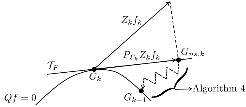
Figure 1: A single iteration of Algorithm 5.

Input: $A,B,\Lambda,\bar{\mathsf{F}},G_{0},iter_{max}.$

Output: Local minimum $(\hat{F},\hat{X})$ of (2).

Initialize: $(F_{0},X_{0})\leftarrow\text{Algorithm }\ref{algo:sp_EAP2}(A,B,\Lambda,\bar{\mathsf{F}},G_{0},iter_{max})$, $G_{0}\leftarrow F_{0}X_{0}$, $i\leftarrow 0$

repeat

       $\alpha\leftarrow$ Update step size;

       $g_{ns}\leftarrow g-\alpha P_{F}Z(F,X)f$;

       $X_{ns}\leftarrow$ Solution of Sylvester equation (16a);

       $F_{ns}\leftarrow G_{ns}X_{ns}^{-1}$;

      1 $(F,X)\leftarrow\text{Algorithm \ref{algo:sp_EAP2}}(A,B,\Lambda,\bar{\mathsf{F}},G_{ns},iter_{max})$;

       $G\leftarrow FX$;

       $i\leftarrow i+1$;

      

until convergence or $i>iter_{max}$;

return $(F,X)$

Algorithm 5 Sparse solution to the MGEAP

Algorithm 5 is computationally intensive due to the use of Algorithm 4 in step 5 to compute the projection on the space of sparse matrices. In fact, the computational complexity of Algorithm 5 is one order higher than that of non-sparse MGEAP Algorithm 1. However, a way to considerably reduce the number of iterations of Algorithm 5 is to initialize it using the approximately-sparse solution obtained by Algorithm 2. In this case, Algorithm 5 starts near the the local minimum and, thus, its convergence time reduces considerably.

V Simulation studies

In this section, we present the implementation details of the algorithms developed in Section IV and provide numerical simulations to illustrate their properties.

V-A Implementation aspects of the algorithms

In the Newton descent step (step 1) of Algorithm 1, we need to choose (omitting the parameter dependence notation) $V$ such that $H+V$ is positive-definite. We choose $V=\delta I_{mn}-Z_{1}Z^{\mathsf{T}}-ZZ_{1}^{\mathsf{T}}$ where, $0<\delta\ll 1$. Thus, from (11), we have: $H+V=ZZ^{\mathsf{T}}+\epsilon I_{mn}$. Clearly, $ZZ^{\mathsf{T}}$ is positive-semidefinite and the small additive term $\epsilon I_{mn}$ ensures that $H+V$ is positive-definite. Note that other possible choices of $V$ also exist. In step 1 of Algorithm 1, we use the Armijo rule to compute the step size $\alpha$. Finally, we use $\left\lVert\frac{dJ}{dg}\right\rVert_{2}<\epsilon$, $0<\epsilon\ll 1$ as the convergence criteria of Algorithm 1. For Algorithm 2, we analogously choose $V_{W}=\delta I_{mn}-Z_{1,W}Z^{\mathsf{T}}-ZZ_{1,W}^{\mathsf{T}}$ and the same convergence criteria and step size rule as Algorithm 1. In both algorithms, if we encounter a scenario in which the solution $X$ of (16a) is singular (c.f. paragraph below (16b)), we perturb $G$ slightly such that the new solution is non-singular, and then continue the iterations. We remark that such instances occur extremely rarely in our simulations.

For the sparse EAP Algorithm 3, we use the convergence criteria $e_{X}=\lVert[I_{n^{2}}-\tilde{B}(X)(\tilde{B}(X))^{+}]\tilde{a}(x)\rVert_{2}<\epsilon$, $0<\epsilon\ll 1$. For Algorithm 4, we use the convergence criteria $e_{F}=\lVert F-\bar{\mathsf{F}}\circ F\rVert_{F}<\epsilon$, $0<\epsilon\ll 1$. Thus, the iterations of these algorithms stop when $x$ lies in a certain subspace and when the sparsity error becomes sufficiently small (within the specified tolerance), respectively. Further, note that Algorithm 4 uses Algorithm 1 in step 4 without specifying an initial condition $G_{0}$ for the latter. This is because in step 4, we effectively run Algorithm 1 for multiple initial conditions in order to capture its global minima. We remark that the capture of global minima by Algorithm 1 is crucial for convergence of Algorithm 4.

As the iterations of Algorithm 4 progress, the sparse matrix $F$ achieves eigenvalue assignment with increasing accuracy. As a result, near the convergence of Algorithm 4, the eigenvalues of $A+BF$ and $\Lambda$ are very close to each other. This creates numerical difficulties when Algorithm 1 is used with parameters $(A+BF,B,\Lambda)$ in step 4 (see Assumption 4). To avoid this issue, we run Algorithm 1 using a preliminary feedback $F_{p}$, as explained below Assumption 4.

Finally, for Algorithm 5, we use the following convergence criteria: $\left\lVert P_{F}\frac{dJ}{dg}\right\rVert_{2}<\epsilon$, $0<\epsilon\ll 1$. We choose the stopping tolerance $\epsilon$ between $10^{-6}$ and $10^{-5}$ for all the algorithms.

V-B Numerical study

We begin this subsection with the following example:

$$\small A =\begin{bmatrix}-3.7653&-2.1501&\phantom{-}0.3120&-0.2484\\ \phantom{-}1.6789&\phantom{-}1.0374&-0.5306&\phantom{-}1.3987\\ -2.1829&-2.5142&-1.2275&\phantom{-}0.2833\\ -13.6811&-9.6804&-0.5242&\phantom{-}2.9554\end{bmatrix}\!,$$

$$\small B =\begin{bmatrix}1&1&2&5\\ 1&3&4&2\end{bmatrix}^{\mathsf{T}}\!\!\!\!,\qquad\bar{\mathsf{F}}=\begin{bmatrix}1&1&0&0\\ 1&0&1&1\end{bmatrix}\!,$$

$$\mathcal{S} =\{-2,-1,-0.5\pm j\}.$$

TABLE I: Comparison of MGEAP solutions by Algorithms 1, 2 and 5

Non-sparse solutions by Algorithm 1

$\hat{X}_{1}=\begin{bmatrix}-0.0831+0.3288j&\hbox{\multirowsetup$\hat{x}_{1}^{*}$}&-0.5053&\phantom{-}0.2031\\ \phantom{-}0.1919-0.4635j&&\phantom{-}0.5612&-0.2505\\ \phantom{-}0.1603+0.5697j&&\phantom{-}0.5617&\phantom{-}0.8441\\ \phantom{-}0.3546+0.3965j&&-0.3379&\phantom{-}0.4283\end{bmatrix}$

$\hat{L}_{1}=\>\begin{bmatrix}-0.5569+1.4099j&\hbox{\multirowsetup\phantom{-}$\hat{l}_{1}^{*}$\phantom{-}}&-0.9154&\phantom{-}2.5568\\ -0.2967+1.0244j&&-0.5643&\phantom{-}1.7468\\ -0.0687+0.0928j&&\phantom{-}0.0087&\phantom{-}0.2722\\ \phantom{-}0.2259-0.2523j&&\phantom{-}0.0869&-0.4692\end{bmatrix}$

$\hat{F}_{1}=\begin{bmatrix}-0.1111&-0.1089&-0.0312&-0.4399\\ -0.1774&-0.2072&\phantom{-}0.0029&\phantom{-}0.1348\end{bmatrix}$, $\lVert\hat{F}_{1}\rVert_{F}=0.5580$

$\hat{F}_{2}=\begin{bmatrix}\phantom{-}0.3817&-0.3349&\phantom{-}0.7280&-0.2109\\ -0.0873&-0.4488&-0.4798&-0.0476\end{bmatrix}$, $\lVert\hat{F}_{2}\rVert_{F}=1.1286$

$\hat{F}_{3}=\begin{bmatrix}0.3130&\phantom{-}2.0160&\phantom{-}1.2547&-0.6608\\ 0.0683&-0.7352&-0.0748&-1.0491\end{bmatrix}$, $\lVert\hat{F}_{3}\rVert_{F}=2.7972$

Average # of Steepest/Newton descent iterations = $5402.1/15.5$

Approximately-sparse solutions by Algorithm 2 with $\mathbf{w=30}$

$\hat{F}_{1}=\begin{bmatrix}0.9652&-1.3681&\phantom{-}0.0014&-0.0021\\ 0.4350&-0.0023&-0.6746&-0.1594\end{bmatrix}$, $\lVert\hat{F}_{1}\rVert_{F}=1.8636$

$\hat{F}_{2}=\begin{bmatrix}-1.0599&-1.7036&-0.0013&-0.0071\\ -0.1702&-0.0057&\phantom{-}0.0263&-0.0582\end{bmatrix}$, $\lVert\hat{F}_{2}\rVert_{F}=2.0146$

$\hat{F}_{3}=\begin{bmatrix}\phantom{-}3.3768&\phantom{-}2.2570&0.0410&-0.0098\\ -1.4694&-0.0061&0.1242&-3.8379\end{bmatrix}$, $\lVert\hat{F}_{3}\rVert_{F}=5.7795$

Average # of Newton descent iterations = $19.1$

Sparse solutions by Algorithm 5

$\hat{X}_{1}=\begin{bmatrix}-0.3370+0.3296i&\hbox{\multirowsetup$\hat{x}_{1}^{*}$}&-0.4525&\phantom{-}0.5168\\ \phantom{-}0.2884-0.1698i&&\phantom{-}0.1764&-0.3007\\ -0.4705+0.5066i&&-0.7478&\phantom{-}0.7831\\ \phantom{-}0.2754+0.3347i&&-0.4527&\phantom{-}0.1711\end{bmatrix}$

$\hat{L}_{1}=\begin{bmatrix}\phantom{-}25.2072+16.5227i&\hbox{\multirowsetup$\hat{l}_{1}^{*}$}&\phantom{-}44.6547&\phantom{-}82.3616\\ \phantom{-}11.0347+11.8982i&&\phantom{-}12.5245&\phantom{-}35.8266\\ -12.2600-5.8549i&&-24.5680&-39.1736\\ -0.6417-2.2060i&&-0.4383&-3.6464\end{bmatrix}$

$\hat{F}_{1}=\begin{bmatrix}0.9627&-1.3744&\phantom{-}0.0000&\phantom{-}0.0000\\ 0.4409&\phantom{-}0.0000&-0.6774&-0.1599\end{bmatrix}$, $\lVert\hat{F}_{1}\rVert_{F}=1.8694$

$\hat{F}_{2}=\begin{bmatrix}-1.0797&-1.7362&0.0000&\phantom{-}0.0000\\ -0.1677&\phantom{-}0.0000&0.0264&-0.0610\end{bmatrix}$, $\lVert\hat{F}_{2}\rVert_{F}=2.0525$

$\hat{F}_{3}=\begin{bmatrix}\phantom{-}3.4465&\phantom{-}2.2568&0.0000&\phantom{-}0.0000\\ -1.8506&-0.0000&0.3207&-4.0679\end{bmatrix}$, $\lVert\hat{F}_{3}\rVert_{F}=6.0866$

Average # of Newton descent iterations:

1. Using random initialization = $8231$

2. Using initialization by Algorithm 2 = $715$

The eigenvalues of $A$ are $\Gamma(A)=\{-2,-1,1\pm 2j\}$. Thus, the feedback $F$ is required to move two unstable eigenvalues into the stable region while keeping the other two stable eigenvalues fixed. Table I shows the non-sparse, approximately-sparse and sparse solutions obtained by Algorithms 1, 2 and 5, respectively, and Figure 2 shows a sample iteration run of these algorithms. Since the number of iterations taken by the algorithms to converge depends on their starting points, we report the average number of iterations taken over $1000$ random starting points. Further, to obtain approximately-sparse solutions, we use the weighing matrix with $W_{ij}=w$ if $\bar{\mathsf{F}}_{ij}=1$. All the algorithms obtain three local minima, among which the first is the global minimum. The second column in $\hat{X}$ and $\hat{L}$ is conjugate of the first column (c.f. Remark 2). It can be verified that the non-sparse and sparse solutions satisfy the optimality conditions of Theorem 4.

For the non-sparse solution, the number of iterations taken by Algorithm 1 with steepest descent are considerably larger than the Newton descent. This is because the steepest descent converges very slowly near a local minimum. Therefore, we use Newton descent steps in Algorithms 1 and 2. Next, observe that the entries at the sparsity locations of the locally minimum feedbacks obtained by Algorithm 2 have small magnitude. Further, the average number of Newton descent iterations for convergence and the norm of the feedback obtained of Algorithm 2 is larger as compared to Algorithm 1. This is because the approximately-sparse optimization problem (25) is effectively more restricted than its non-sparse counterpart (16).

Finally, observe that the solutions of Algorithm 5 are sparse. Note that Algorithm 5 involves the use of projection Algorithm 4, which in turn involves running Algorithm 1 multiple times. Thus, for a balanced comparison, we present the total number of Newton descent iterations of Algorithm 1 involved in the execution of Algorithm 5. From Table I, we can observe that Algorithm 5 involves considerably more Newton descent iterations compared to Algorithms 1 and 2, since it involves computationally intensive projection calculations by Algorithm 4. One way to reduce its computation time is to initialize is near the local minimum using the approximately sparse solution of Algorithm 2.

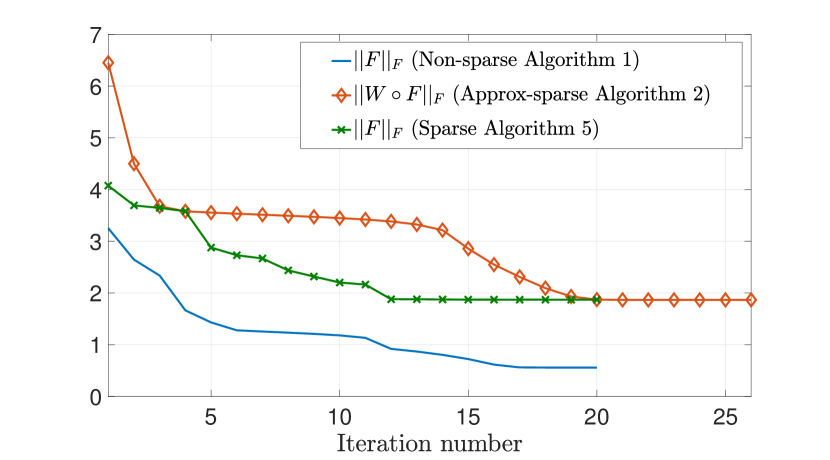
Figure 2: Optimization costs for a sample run of Algorithms 1, 2 and 5 (the algorithms converge to their global minima). For Algorithm 5, number of outer iterations are reported.

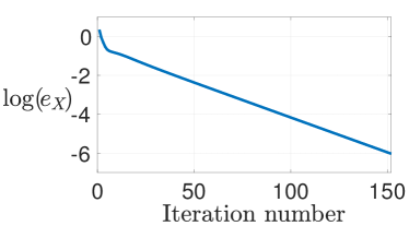
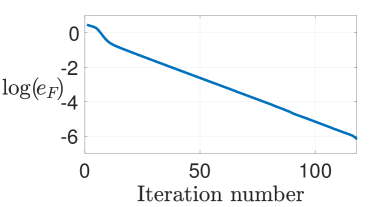
Figure 3: Projection and sparsity errors for a sample run of (a) Algorithm 3 and (b) Algorithm 4, respectively.

Figure 3 shows a sample run of EAP Algorithms 3 and 4 for $G_{0}=\left[\begin{smallmatrix}-1.0138&\phantom{-}0.6851&-0.1163&0.8929\\ -1.8230&-2.2041&-0.1600&0.7293\end{smallmatrix}\right]$. The sparse feedback obtained by Algorithms 3 and 4 are $F=\left[\begin{smallmatrix}\phantom{-}0.1528&-2.6710&0.0000&\phantom{-}0.0000\\ -0.8382&\phantom{-}0.0000&0.1775&-0.1768\end{smallmatrix}\right]$ and $F=\left[\begin{smallmatrix}\phantom{-}4.2595&4.2938&\phantom{-}0.0000&\phantom{-}0.0000\\ -0.2519&0.0000&-2.1258&-1.3991\end{smallmatrix}\right]$, respectively. The projection error $e_{X}$ and the sparsity error $e_{F}$ capture the convergence of Algorithms 3 and 4, respectively. Figure 3 shows that these errors decrease, thus indicating convergence of the algorithms.

Next, we provide an empirical verification of the convergence of heuristic Algorithms 3 and 4. Let the sparsity ratio ($SR$) be defined as the ratio of the number of sparse entries to the total number of entries in $F$ (i.e. $SR=\frac{\text{Number of }0^{\prime}s\text{ in }\bar{\mathsf{F}}}{mn}$). We perform $1000$ random executions of both the algorithms. In each execution, $n$ is randomly selected between $4$ and $20$ and $m$ is randomly selected between $2$ and $n$. Then, matrices $(A,B)$ are randomly generated with appropriate dimensions. Next, a binary sparsity pattern matrix $\bar{\mathsf{F}}$ is randomly generated with the number of sparsity entries given by $\lfloor SR\times mn\rfloor$, where $\lfloor\cdot\rfloor$ denotes rounding to the next lowest integer. To ensure feasibility (c.f. Assumption 2 and discussion below), we pick the desired eigenvalue set $\mathcal{S}$ randomly as follows: we select a random $F_{r}$ which satisfies the selected sparsity pattern $\bar{\mathsf{F}}$, and select $\mathcal{S}=\Gamma(A+BF_{r})$. Finally, we set $iter_{max}=1000$ and select a random starting point $G_{0}(F_{0},X_{0})$, and run both algorithms from the same starting point. Let $F_{sol}$ denote the feedback solution obtained by Algorithms 3 and 4, respectively, and let $d_{F_{sol},F_{0}}\triangleq\lVert F_{sol}-F_{0}\rVert_{F}$ denote the distance between the starting point $F_{0}$ and the final solution. Since Algorithm 4 is a projection algorithm, the metric $d_{F_{sol},F_{0}}$ captures its projection performance.

TABLE II: Convergence properties of EAP Algorithms 3 and 4

$\mathbf{SR}$	Algorithm 3	Algorithm 4
$1/4$	Convergence instances = 427	Convergence instances = 997
	Average $d_{F_{sol},F_{0}}$ = 8.47	Average $d_{F_{sol},F_{0}}$ = 1.28
$1/2$	Convergence instances = 220	Convergence instances = 988
	Average $d_{F_{sol},F_{0}}$ = 4.91	Average $d_{F_{sol},F_{0}}$ = 1.61
$2/3$	Convergence instances = 53	Convergence instances = 983
	Average $d_{F_{sol},F_{0}}$ = 6.12	Average $d_{F_{sol},F_{0}}$ = 1.92

Table II shows the convergence results of Algorithms 3 and 4 for three different sparsity ratios. While the convergence of Algorithm 3 deteriorates as $F$ becomes more sparse, Algorithm 4 converges in almost all instances. This implies that in the context of Algorithm 5, Algorithm 4 provides a valid projection in step 5 in almost all instances. We remark that in the rare case that Algorithm 4 fails to converge, we can reduce the step size $\alpha$ to obtain a new $G_{ns}$ and compute its projection. Further, we compute the average of distance $d_{F_{sol},F_{0}}$ over all executions of the Algorithms 3 and 4 that converge. Observe that the average distance for Algorithm 4 is smaller than Algorithm 3. This shows that Algorithm 4 provides considerably better projection of $F_{0}$ in the space of sparse matrices as compared to Algorithm 3 (c.f. Remark 15). Note that the above simulations focus on the convergence properties as $SR$ changes and they do not capture the individual effects of the number of sparsity constraints, $m$ and $n$ (for instance, small systems versus large systems).

VI Feasibility of the sparse EAP

In this section we provide a discussion of the feasibility of the sparse EAP, i.e., eigenvalue assignment with sparse, static state feedback. We address certain aspects of this problem, and leave a detailed characterization for future research.

Lemma 16.

(NP-hardness) Determining the feasibility of the sparse EAP is NP-hard.

Proof.

We prove the result using the NP-hardness property of the static output feedback pole placement (SOFPP) problem [53], which is stated as follows: for a given $A\in\mathbb{R}^{n\times n}$, $B\in\mathbb{R}^{n\times m}$, and $C\in\mathbb{R}^{p\times n}$, determine if there exists a non-sparse $K\in\mathbb{R}^{m\times p}$ such that the eigenvalues of $A+BKC$ are at some desired locations. Without loss of generality, we assume that $C$ is full row rank. Thus, there exists an invertible $T=\begin{bmatrix}C^{+}&V\end{bmatrix}\in\mathbb{R}^{n\times n}$ with $CV=0$. Taking the similarity transformation by $T$ (which preserves the eigenvalues) we get

$$T^{-1}(A+BKC)T=\underbrace{T^{-1}AT}_{\bar{A}}+\underbrace{T^{-1}B}_{\bar{B}}\begin{bmatrix}K&0\end{bmatrix}.$$

Clearly, the above SOFPP problem is equivalent to a sparse EAP with matrices $\bar{A},\bar{B}$ and sparsity pattern given by $\bar{F}=\begin{bmatrix}1_{m\times p}&0_{m\times(n-p)}\end{bmatrix}$. Thus, the NP-hardness of the sparse EAP follows form the NP-hardness of the SOFPP problem. ∎

Next, we present graph-theoretic necessary and sufficient conditions for arbitrary eigenvalue assignment by sparse static feedback. Due to space constraints, we briefly introduce the required graph-theoretic notions and refer the reader to [54] for more details. Given a square matrix $A=[a_{ij}]\in\mathbb{R}^{n\times n}$, let $\mathcal{G}_{A}$ denote its associated graph with $n$ vertices, and let $a_{ij}$ be the weight of the edge from vertex $j$ to vertex $i$. A closed directed path (sequence of consecutive vertices) is called a cycle if the start and end vertices coincide, and no vertex appears more than once along the path (except for the first vertex). A set of vertex disjoint cycles is called a cycle family. The width of a cycle family is the number of edges contained in all its cycles.

Lemma 17.

(Necessary conditions) Let $H=\left[\begin{smallmatrix}A&B\\ F&0\end{smallmatrix}\right]$, and let $\mathcal{G}_{H}$ be its associated graph. Let $n_{s}$ be the number of sparsity constraints (zero entries) in the feedback matrix $F\in\mathbb{R}^{m\times n}$. Further, let $S_{k}$ denote the set of cycle families of $\mathcal{G}_{H}$ of width $k$, with $k=1,\dots,n$. Necessary conditions for arbitrary eigenvalue assignment with sparse, static state feedback are:

1. $n_{s}\leq(m-1)n$, that is, $F$ has at least $n$ nonzero entries,

2. for each $k=1,\cdots,n$, there exist a nonzero entry $f_{i_{k}j_{k}}$ of $F$ such that its corresponding edge appears in $S_{k}$.

Proof.

(i) Arbitrary eigenvalue assignment requires that the feedback $F$ should assign all the $n$ coefficients of the characteristic polynomial $\text{det}(sI-A-BF)$ to arbitrary values. This requires the mapping $h:\mathbb{R}^{mn-n_{s}}\rightarrow\mathbb{R}^{n}$ from the nonzero entries of $F$ to the coefficients of the characteristic polynomial to be surjective, which imposes that the dimension of the domain of $h$ should not be less that the dimension of its codomain.

(ii) Let $c_{k}$, $k=1,\dots,n$ denote the coefficients of the polynomial det($sI-A-BF$). Then, $c_{k}$ is a multiaffine function of the nonzero entries of $F$, which appear in the cycle families in $S_{k}$ [54]. If there exists no feedback edge in $S_{k}$, then $c_{k}$ is fixed and does not depend on $F$. Thus, arbitrary eigenvalue assignment is not possible in this case. ∎

Lemma 18.

(Sufficient conditions) Let $H=\left[\begin{smallmatrix}A&B\\ F&0\end{smallmatrix}\right]$, and let $\mathcal{G}_{H}$ be its associated graph. Let $S_{k}$ denote the set of cycle families of $\mathcal{G}_{H}$ of width $k$, and let $F_{k}$ denote the set of feedback edges contained in $S_{k}$, with $k=1,\dots,n$. Then, each of the following conditions is sufficient for arbitrary eigenvalue assignment with sparse, static state feedback:

1. for each $k=1,\cdots,n$, there exist a feedback edge that appears in $S_{k}$ and not in $S_{j}$, for all $j\neq k$,

2. there exists a permutation $\{i_{1},i_{2},\cdots,i_{n}\}$ of $\{1,2,\cdots,n\}$ such that $\emptyset\neq F_{i_{1}}\subset F_{i_{2}}\subset\cdots\subset F_{i_{n}}$.

Proof.

(i) Similar to the proof of Lemma 17, if there exist a nonzero entry $f_{i_{k}j_{k}}$ that is exclusive to $S_{k}$, then such variable can be used to assign $c_{k}$ arbitrarily. If this holds for $k=1,\dots,n$, then all coefficients of the characteristic polynomial can be assigned arbitrarily, resulting in arbitrary eigenvalue assignment.

(ii) Condition (ii) guarantees that, for $j=2,\cdots,n$, the coefficient $c_{i_{j}}$ depends on the feedback variables of $c_{i_{j-1}}$ and on some additional feedback variables. These additional variables can be used to assign the coefficient $c_{i_{j}}$ arbitrarily. ∎

To illustrate the results, consider the following example:

$$A=\begin{bmatrix}a_{11}&a_{12}&0\\ 0&0&0\\ a_{31}&0&0\end{bmatrix},B=\begin{bmatrix}b_{11}&0\\ 0&b_{22}\\ 0&0\end{bmatrix},F=\begin{bmatrix}f_{11}&0&0\\ f_{21}&0&f_{23}\end{bmatrix}.$$

The corresponding graph and cycle families are shown in Fig. 4. Note that the edges $f_{11},f_{21}$ and $f_{23}$ are exclusive to cycle families of widths $1,2$ and $3$, respectively. Thus, condition (i) of Lemma 18 is satisfied and arbitrary eigenvalue assignment is possible. Next, consider the feedback $F=\left[\begin{smallmatrix}0&0&f_{13}\\ f_{21}&f_{22}&0\end{smallmatrix}\right]$. In this case, the sets of feedback edges in the family cycles of different widths are $F_{1}=\{f_{22}\},F_{2}=\{f_{22},f_{13},f_{21}\}$ and $F_{3}=\{f_{22},f_{13}\}$. We observe that $F_{1}\subset F_{3}\subset F_{2}$ (condition (ii) of Lemma 18) and arbitrary eigenvalue assignment is possible. Further, if $F=\left[\begin{smallmatrix}0&f_{12}&f_{13}\\ f_{21}&0&0\end{smallmatrix}\right]$, then $F_{1}=F_{3}=\emptyset$, and the coefficients $c_{1}$, $c_{3}$ of $\text{det}(sI-A-BF)$ are fixed. This violates condition (ii) of Lemma 17 and prevents arbitrary eigenvalue assignment with the given $F$.

Note that the conditions in Lemmas 17 and 18 are constructive, and can also be used to determine a sparsity pattern that guarantees feasibility of the sparse EAP. We leave the design of such algorithm as a topic of future investigation.

Remark 19.

(Comparison with exiting results) We emphasize that the conditions presented in Lemmas 17 and 18 for arbitrary eigenvalue assignment using static state feedback are not equivalent to the conditions for non-existence of SFMs studied in [27], [31, 32, 33, 34, 35], [38]. The reason is that arbitrary assignment of non-SFMs necessarily requires a dynamic controller and cannot, in general, be achieved by a static controller. Further, our graph-theoretic results are based on the feedback edges being suitably covered by cycle families, whereas the results in [32, 33] are based on the state nodes/subgraphs being suitably covered by strong components, cycles/cactus. $\square$

(a) Graph $\mathcal{G}_{H}$, where blue and orange nodes correspond to state and control vertices, respectively.

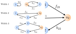
(b) Cycle families of $\mathcal{G}_{H}$. All cycle families contain a single cycle. There are two cycle families of width $1$, and one cycle family each of width $2$ and $3$.

Figure 4: Graph $\mathcal{G}_{H}$ and its cycle families. $u_{1}$, $u_{2}$ denote the control vertices.

VII Conclusion

In this paper we studied the MGEAP for LTI systems with arbitrary sparsity constraints on the static feedback matrix. We presented an analytical characterization of its locally optimal solutions, thereby providing explicit relations between an optimal solution and the eigenvector matrices of the associated closed loop system. We also provided a geometric interpretation of an optimal solution of the non-sparse MGEAP. Using a Sylvester-based parametrization, we developed a heuristic projected gradient descent algorithm to obtain local solutions to the MGEAP. We also presented two novel algorithms for solving the sparse EAP and an algorithm to obtain approximately sparse local solution to the MGEAP. Numerical studies suggest that our heuristic algorithm converges in most cases. Further, we also discussed the feasibility of the sparse EAP and provided necessary and sufficient conditions for the same.

The analysis in the paper is developed, for the most part, under the assumption that the sparse EAP problem with static feedback is feasible. A future direction of research includes a more detailed characterization of the feasibility of the EAP, a constructive algorithm to determine feasible sparsity patterns, a convex relaxation of the sparse MGEAP with guaranteed distance from optimality, and a more rigorous analysis of convergence of Algorithms 4 and 5.

References

• [1] R. Schmid, L. Ntogramatzidis, T. Nguyen, and A. Pandey. A unified method for optimal arbitrary pole placement. Automatica, 50(8):2150–2154, 2014.
• [2] Y. Peretz. On parametrization of all the exact pole-assignment state-feedbacks for LTI systems. IEEE Transactions on Automatic Control, 62(7):3436–3441, 2016.
• [3] P. J. Antsaklis and A. N. Michael. Linear systems. Birkhauser, 2005.
• [4] J. Kautsky, N. K. Nichols, and P. Van Dooren. Robust pole assignment in linear state feedback. International Journal of Control, 44(5):1129–1155, 1985.
• [5] A. Pandey, R. Schmid, and T. Nguyen. Performance survey of minimum gain exact pole placement methods. In European Control Conference, pages 1808–1812, Linz, Austria, 2015.
• [6] Y. J. Peretz. A randomized approximation algorithm for the minimal-norm static-output-feedback problem. Automatica, 63:221–234, 2016.
• [7] B. Bamieh, F. Paganini, and M. A. Dahleh. Distributed control of spatially invariant systems. IEEE Transactions on Automatic Control, 47(7):1091–1107, 2002.
• [8] M. Rotkowitz and S. Lall. A characterization of convex problems in decentralized control. IEEE Transactions on Automatic Control, 51(2):274–286, 2006.
• [9] A. Mahajan, N. C. Martins, M. C. Rotkowitz, and S. Yuksel. Information structures in optimal decentralized control. In IEEE Conf. on Decision and Control, pages 1291–1306, Maui, HI, USA, December 2012.
• [10] F. Lin, M. Fardad, and M. R. Jovanović. Augmented Lagrangian approach to design of structured optimal state feedback gains. IEEE Transactions on Automatic Control, 56(12):2923–2929, 2011.
• [11] R. Schmid, A. Pandey, and T. Nguyen. Robust pole placement with moore’s algorithm. IEEE Transactions on Automatic Control, 59(2):500–505, 2014.
• [12] M. Ait Rami, S. E. Faiz, A. Benzaouia, and F. Tadeo. Robust exact pole placement via an LMI-based algorithm. IEEE Transactions on Automatic Control, 54(2):394–398, 2009.
• [13] R. Byers and S. G. Nash. Approaches to robust pole assignment. International Journal of Control, 49(1):97–117, 1989.
• [14] A. Varga. Robust pole assignment via Sylvester equation based state feedback parametrization. In IEEE International Symposium on Computer-Aided Control System Design, Anchorage, AK, USA, 2000.
• [15] E. K. Chu. Pole assignment via the Schur form. Systems & Control Letters, 56(4):303–314, 2007.
• [16] A. L. Tits and Y. Yang. Globally convergent algorithms for robust pole assignment by state feedback. IEEE Transactions on Automatic Control, 41(10):1432–1452, 1996.
• [17] E. K. Chu. Optimization and pole assignment in control system design. International Journal of Applied Mathematics and Computer Science, 11(5):1035–1053, 2001.
• [18] A. Pandey, R. Schmid, T. Nguyen, Y. Yang, V. Sima, and A. L. Tits. Performance survey of robust pole placement methods. In IEEE Conf. on Decision and Control, pages 3186–3191, Los Angeles, CA, USA, 2014.
• [19] B. A. White. Eigenstructure assignment: a survey. Proceedings of the Institution of Mechanical Engineers, 209(1):1–11, 1995.
• [20] L. F. Godbout and D. Jordan. Modal control with feedback-gain constraints. Proceedings of the Institution of Electrical Engineers, 122(4):433–436, 1975.
• [21] B. Kouvaritakis and R. Cameron. Pole placement with minimised norm controllers. IEE Proceedings D - Control Theory and Applications, 127(1):32–36, 1980.
• [22] H. K. Tam and J. Lam. Newton’s approach to gain-controlled robust pole placement. IEE Proceedings - Control Theory and Applications, 144(5):439–446, 1997.
• [23] A. Varga. A numerically reliable approach to robust pole assignment for descriptor systems. Future Generation Computer Systems, 19(7):1221–1230, 2003.
• [24] A. Varga. Robust and minimum norm pole assignment with periodic state feedback. IEEE Transactions on Automatic Control, 45(5):1017–1022, 2000.
• [25] S. Datta, B. Chaudhuri, and D. Chakraborty. Partial pole placement with minimum norm controller. In IEEE Conf. on Decision and Control, pages 5001–5006, Atlanta, GA, USA, 2010.
• [26] S. Datta and D. Chakraborty. Feedback norm minimization with regional pole placement. International Journal of Control, 87(11):2239–2251, 2014.
• [27] S. H. Wang and E. J. Davison. On the stabilization of decentralized control systems. IEEE Transactions on Automatic Control, 18(5):473–478, 1973.
• [28] J. P. Corfmat and A. S. Morse. Decentralized control of linear multivariable systems. Automatica, 12(5):479–495, 1976.
• [29] B. D. O. Anderson and D. J. Clements. Algebraic characterization of fixed modes in decentralized control. Automatica, 17(5):703–712, 1981.
• [30] E. J. Davison and U. Ozguner. Characterizations of decentralized fixed modes for interconnected systems. Automatica, 19(2):169–182, 1983.
• [31] M. E. Sezer and D. D. Siljak. Structurally fixed modes. Systems & Control Letters, 1(1):60–64, 1981.
• [32] V. Pichai, M. E. Sezer, and D. D. Siljak. A graph-theoretic characterization of structurally fixed modes. Automatica, 20(2):247–250, 1984.
• [33] V. Pichai, M. E. Sezer, and D. D. Siljak. A graphical test for structurally fixed modes. Mathematical Modelling, 4(4):339–348, 1983.
• [34] A. Alavian and M. Rotkowitz. Fixed modes of decentralized systems with arbitrary information structure. In International Symposium on Mathematical Theory of Networks and Systems, pages 913–919, Groningen, The Netherlands, 2014.
• [35] A. Alavian and M. Rotkowitz. Stabilizing decentralized systems with arbitrary information structure. In IEEE Conf. on Decision and Control, pages 4032–4038, Los Angeles, CA, USA, 2014.
• [36] S. Pequito, G. Ramos, S. Kar, A. P. Aguiar, and J. Ramos. The robust minimal controllability problem. Automatica, 82:261–268, 2017.
• [37] S. Pequito, S. Kar, and A. P. Aguiar. A framework for structural input/output and control configuration selection in large-scale systems. IEEE Transactions on Automatic Control, 61(2):303–318, 2016.
• [38] S. Moothedath, P. Chaporkar, and M. N. Belur. Minimum cost feedback selection for arbitrary pole placement in structured systems. IEEE Transactions on Automatic Control, 63(11):3881–3888, 2018.
• [39] Petersen K. B. and M. S. Pedersen. The Matrix Cookbook. Technical University of Denmark, 2012.
• [40] J. R. Magnus and H. Neudecker. Matrix Differential Calculus with Applications in Statistics and Econometrics. John Wiley and Sons, 1999.
• [41] D. Kressner and M. Voigt. Distance problems for linear dynamical systems. In Numerical Algebra, Matrix Theory, Differential-Algebraic Equations and Control Theory, pages 559–583. Springer, 2015.
• [42] J. Rosenthal and J. C. Willems. Open problems in the area of pole placement. In Open Problems in Mathematical Systems and Control Theory, page 181–191. Springer, 1999.
• [43] J. Leventides and N. Karcanias. Sufficient conditions for arbitrary pole assignment by constant decentralized output feedback. Mathematics of Control, Signals and Systems, 8(3):222–240, 1995.
• [44] D. G. Luenberger and Y. Ye. Linear and Nonlinear Programming. Springer, 2008.
• [45] P. A. Absil, R. Mahony, and R. Sepulchre. Optimization Algorithms on Matrix manifolds. Princeton University Press, 2008.
• [46] P Lancaster. The Theory of Matrices. American Press, 1985.
• [47] J. H. Wilkinson. The Algebraic Eigenvalue Problem. Clarendon Press, 1988.
• [48] S. P. Bhattacharyya and E. De Souza. Pole assignment via Sylvester’s eqauation. Systems & Control Letters, 1(4):261–263, 1982.
• [49] N. J. Hingham. Accuracy and Stability of Numerical Algorithms. SIAM, 2002.
• [50] S. P. Bhattacharyya and E. De Souza. Controllability, observability and the solution of AX-XB=C. Linear algebra and its applications, 39(1):167–188, 1981.
• [51] R. Escalante and M. Raydan. Alternating Projection Methods. SIAM, 2011.
• [52] A. S. Lewis and J. Malick. Alternating projections on manifolds. Mathematics of Operations Research, 33(1):216–234, 2008.
• [53] M. Fu. Pole placement via static output feedback is NP-hard. IEEE Transactions on Automatic Control, 49(5):855–857, 2004.
• [54] K. J. Reinschke. Multivariable Control: A Graph-Theoretic Approach. Springer, 1988.