RR Lyrae stars as standard candles in the Gaia Data Release 2 Era

Abstract

We present results from the analysis of 401 RR Lyrae stars (RRLs) belonging to the field of the Milky Way (MW). For a fraction of them multi-band ($V$, $K_{\mathrm{s}}$, $W1$) photometry, metal abundances, extinction values and pulsation periods are available in the literature and accurate trigonometric parallaxes measured by the Gaia mission alongside Gaia $G$-band time-series photometry have become available with the Gaia second data release (DR2) on 2018 April 25. Using a Bayesian fitting approach we derive new near-, mid-infrared period-absolute magnitude-metallicity ($PMZ$) relations and new absolute magnitude-metallicity relations in the visual ($M_{V}-{\rm[Fe/H]}$) and $G$ bands ($M_{G}-{\rm[Fe/H]}$), based on the Gaia DR2 parallaxes. We find the dependence of luminosity on metallicity to be higher than usually found in the literature, irrespective of the passband considered. Running the adopted Bayesian model on a simulated dataset we show that the high metallicity dependence is not caused by the method, but likely arises from the actual distribution of the data and the presence of a zero-point offset in the Gaia parallaxes. We infer a zero-point offset of $-0.057$ mas, with the Gaia DR2 parallaxes being systematically smaller. We find the RR Lyrae absolute magnitude in the $V$, $G$, $K_{\rm s}$ and $W1$ bands at metallicity of [Fe/H]=$-1.5$ dex and period of $P=0.5238$ days, based on Gaia DR2 parallaxes to be $M_{V}=0.66\pm 0.06$ mag, $M_{G}=0.63\pm 0.08$ mag, $M_{K_{\rm s}}=-0.37\pm 0.11$ mag and $M_{W1}=-0.41\pm 0.11$ mag, respectively.

1 Introduction

Over the years, many different methods have been devised in order to measure distances in astronomy. However, techniques based on geometrical principles, among which the trigonometric parallax in first place, remain the most direct, simple and reliable tool to anchor the whole astronomical distance ladder on a solid basis. In the distance ladder approach, the limited horizon allowed by parallaxes is circumvented by making use of standard candles, such as, the RR Lyrae (RRL) variable stars, whose absolute calibration rests on parallax measurements of local samples of the class.

RR Lyrae stars (RRLs) are old (age $>10$ Gyr), low mass ($<$ 1 M_⊙), radially pulsating stars which populate the classical instability strip region of the horizontal branch (HB) in the colour-magnitude diagram (CMD). RRLs divide into fundamental (RRab) and first-overtone (RRc) mode pulsators and double-mode (RRd) variables, which pulsate in both modes simultaneously. RRLs serve as standard candles to measure distances since they conform to relations between the absolute visual magnitude and the metallicity ($M_{V}-{\rm[Fe/H]}$), and near- and mid-infrared period-absolute magnitude ($PM$) and $PM$-metallicity ($PMZ$) relations. The near-infrared $PM_{K}Z$ relation has a number of advantages in comparison with the visual ${M_{V}-{\rm[Fe/H]}}$ relation, such as a smaller dependence of the luminosity on interstellar extinction ($A_{K}$=0.114$A_{V}$, Cardelli et al. 1989), metallicity and evolutionary effects. The latter cause an intrinsic spread of the $M_{V}-{\rm[Fe/H]}$ relation of about $\sim 0.2$ mag, while the intrinsic dispersion of the $PMZ$ relation due to evolutionary effects is only 0.04 mag in the $K$ band (Marconi et al., 2015).

The effect of extinction is even less pronounced in the mid-infrared passbands. For instance, the extinction in the Wide-field Infrared Survey Explorer (WISE) $W1$ (3.4 $\mu$m) passband is roughly 15 times smaller than in the $V$ band ($A_{W1}=0.065A_{V}$, Madore et al. 2013). Furthermore, near- and mid-infrared light curves of RRLs have smaller amplitudes, hence, determination of the mean magnitudes is easier and more precise than in visual bands further beating down the dispersion of their fundamental relations. Accurate trigonometric parallaxes for a significantly large sample of RRLs are needed to firmly calibrate their visual $M_{V}-{\rm[Fe/H]}$ and near- and mid-infrared $PMZ$ relations. This is what Gaia, a European Space Agency (ESA) cornerstone mission launched on 2013 December 19, is deemed to provide within a few years time-frame.

Gaia is measuring trigonometric parallaxes, positions, proper motions, photometry and main physical parameters for over a billion stars in the Milky Way (MW) and beyond (Gaia Collaboration et al. 2016a; Gaia Collaboration et al. 2016b). The Gaia first data release (DR1), on 2016 September 14, published positions, parallaxes and proper motions for about 2 million stars in common between Gaia and the Hipparcos and Tycho-2 catalogues, computed as part of the Tycho-Gaia Astrometric Solution (TGAS, Lindegren et al. 2016). The DR1 catalogue comprises parallaxes for 364 MW RRLs, of which a fraction were used by Gaia Collaboration et al. (2017) to calibrate the $M_{V}-{\rm[Fe/H]}$, $PM_{K}Z$ and $PM_{W1}Z$ relations. On 2018 April 25, the Gaia second data release (DR2), has published positions and multi-band photometry for $\sim 1.7$ billion sources as well as parallaxes and proper motions calculated solely on Gaia astrometry for $\sim 1.3$ billion sources (Gaia Collaboration et al., 2018). Gaia DR2 also published a catalogue of more than $\sim$500,000 variable stars of different types (Holl et al., 2018), that comprises 140,784 RRLs (Clementini et al., 2018) for which main characteristic parameters (period, pulsation mode, mean magnitudes and amplitudes in the Gaia $G$, $G_{\rm BP}$ and $G_{\rm RP}$ passbands, extinction and individual metal abundance [Fe/H]) were also released. This provides an enormous contribution to the common knowledge of the variable star population in and beyond the MW and also makes it possible to re-calibrate their fundamental relations and extend them to the Gaia passbands.

A number of independent studies discussing a possible zero-point offset affecting the Gaia DR2 parallaxes appeared recently in the literature (e.g. Arenou et al. 2018; Riess et al. 2018; Zinn et al. 2018; Stassun & Torres 2018). All these studies agree on the Gaia DR2 parallaxes being systematically smaller (hence, providing systematically larger distances) than inferred by other independent techniques.

In this paper we use the accurate parallaxes available with Gaia DR2 for a large sample of local RRLs along with a Bayesian fitting approach to derive new $M_{V}-{\rm[Fe/H]}$, $PM_{K}Z$ and $PM_{W1}Z$ relations, as well as the $G$-band absolute magnitude-metallicity ($M_{G}-{\rm[Fe/H]}$) relation. The new relations are then used to measure RRL absolute magnitudes and the distance to RRLs in the Large Magellanic Cloud (LMC), for which the accuracy of the trigonometric parallax measurements is hampered by the faint magnitude/large distance. In doing so we also test the quality of Gaia DR2 parallaxes and the zero-point parallax offset.

The paper is organised as follows. In Section 2 we describe the sample of RRLs that we have used in this study. In Section 3 we perform a comparison of the DR2 parallaxes with the TGAS, Hipparcos and Hubble Space Telescope (HST) parallaxes and with photometric parallaxes inferred from Baade-Wesselink (BW) studies. The Bayesian fitting approach applied in our study is described in Section 4. The RRL $M_{V}-{\rm[Fe/H]}$, $PM_{K}Z$, $PM_{W1}Z$ and $M_{G}-{\rm[Fe/H]}$ relations derived in this work and a discussion of the Gaia DR2 parallax zero-point offset are presented in Section 5. In Section 6 we use our newly derived relations to measure the distance to the LMC. Finally, a summary of the paper results and main conclusions are presented in Section 7.

2 Data

2.1 The sample of RR Lyrae stars

In order to calibrate the $M_{V}-{\rm[Fe/H]}$, $PM_{K}Z$ and $PM_{W1}Z$ relations of RRL variables, one needs a large sample of RRLs with accurate photometry, the precise knowledge of their period and pulsation mode, metallicities spanning a large enough range, alongside an accurate estimation of the star parallaxes/distances. Following Gaia Collaboration et al. (2017) we select a sample of 403 MW field RRLs studied by Dambis et al. (2013), who have collected and homogenised literature values of period, pulsation mode, extinction in the visual passband ($A_{V}$), metal abundance ([Fe/H]) and intensity-averaged magnitudes in the Johnson V, 2MASS $K_{\mathrm{s}}$ and WISE $W1$ passbands. Dambis et al. (2013) took the pulsation periods from the ASAS3 catalogue (Pojmanski 2002, Maintz 2005) and the General Catalogue of Variable Stars (GCVS, Samus et al. 2007-2015). The intensity-averaged $V$ magnitudes were calculated from nine overlapping sets of observations (see Dambis et al. 2013 and references therein for details); the $K_{\mathrm{s}}$-band intensity-averaged magnitudes were estimated applying a phase-correction procedure described in Feast et al. (2008) to the 2MASS single-epoch $K_{\mathrm{s}}$ measurements of Cutri et al. (2003). Dambis et al. (2013) did not apply phase-corrections to 32 RRLs in their sample. For these objects we adopted the single-epoch $K_{\mathrm{s}}$ magnitudes. According to figure B2 in Feast et al. (2008) the largest amplitude of RRLs in the $K_{\rm s}$ band is $\sim 0.35$ mag. Hence, for the 32 RRLs with single epoch observations we adopt an uncertainty for the mean $K_{\rm s}$ magnitude of 0.175 mag, corresponding to half the maximum amplitude. The intensity-averaged $W1$ magnitudes were estimated by Dambis et al. (2013) from the WISE single-exposure data. Conforming to the referee request an additional uncertainty of 0.02 mag was added to uncertainties in the mean $W1$ magnitudes presented by Dambis et al. (2013).

Table 1: Dataset for the 401 RRLs: (1) name; (2) Gaia identifier; (3) and (4) coordinates in the Gaia DR2 catalogue; (5) Gaia DR2 parallax; (6) RRL type; (7) period; (8), (9) and (10) mean $V$, $K_{\rm s}$ and $W1$ magnitudes from Dambis et al. (2013); (11) mean $G$ magnitude; (12) metallicity on the Zinn & West (1984) metallicity scale; (13) extinction in the $V$ band.

Name	${\rm ID}_{\it Gaia}$	RA	Dec	$\varpi_{\rm DR2}$	Type	P	$V~{}~{}~{}~{}~{}~{}~{}~{}~{}$	$K_{\rm s}$	$W1^{a}$	$G$	[Fe/H]	$A_{V}$
		(deg)	(deg)	(mas)		(day)	(mag)	(mag)	(mag)	(mag)	(dex)	(mag)
DH Peg	2720896455287475584	333.85693	6.82262	2.068 $\pm$ 0.048	Cb	0.2555b	9.553 $\pm$ 0.007	8.603 $\pm$ 0.038	8.551 $\pm$ 0.007		-1.36 $\pm$ 0.20	0.263
DM Cyg	1853751143864356736	320.2981	32.19129	0.965 $\pm$ 0.051	AB	0.4199b	11.530 $\pm$ 0.018	10.287 $\pm$ 0.034	10.228 $\pm$ 0.024	11.43934 $\pm$ 0.00026	-0.14 $\pm$ 0.20	0.300
DH Hya	5737579706158770560	135.06169	-9.779	0.469 $\pm$ 0.040	AB	0.4890b	12.152 $\pm$ 0.009	11.143 $\pm$ 0.039	11.042 $\pm$ 0.028	12.11165 $\pm$ 0.00030	-1.55 $\pm$ 0.20	0.161
DD Hya	3090871397797047296	123.13255	2.83469	0.481 $\pm$ 0.051	AB	0.5018b	12.202 $\pm$ 0.012	11.210 $\pm$ 0.038	11.096 $\pm$ 0.026	12.10446 $\pm$ 0.00024	-1.00 $\pm$ 0.20	0.000
ER Aps	5800912537991603200	265.99488	-76.24484	0.367 $\pm$ 0.015	AB	0.4311b	13.602 $\pm$ 0.018	11.226 $\pm$ 0.037	11.125 $\pm$ 0.006	13.32635 $\pm$ 0.00009	-1.39 $\pm$ 0.20	1.100
DN Aqr	2381771781829913984	349.82189	-24.21641	0.642 $\pm$ 0.051	AB	0.6338b	11.182 $\pm$ 0.008	9.901 $\pm$ 0.037	9.897 $\pm$ 0.022		-1.63 $\pm$ 0.20	0.077
BV Aqr	6820039248616386688	330.72498	-21.52568	0.889 $\pm$ 0.053	C	0.3638	10.888 $\pm$ 0.036	10.010 $\pm$ 0.039	9.975 $\pm$ 0.005		-1.49 $\pm$ 0.20	0.103
AV Ser	4410058473777585024	240.9243	0.59913	0.790 $\pm$ 0.033	AB	0.4876	11.484 $\pm$ 0.009	10.014 $\pm$ 0.037	10.011 $\pm$ 0.015	11.38748 $\pm$ 0.00035	-1.20 $\pm$ 0.20	0.514
VY Lib	6262626680568457600	237.82077	-15.75116	0.788 $\pm$ 0.051	AB	0.5340	11.724 $\pm$ 0.009	10.030 $\pm$ 0.036	10.041 $\pm$ 0.017	11.53776 $\pm$ 0.00025	-1.32 $\pm$ 0.20	0.588
AF Vel	5360400630327427072	163.26066	-49.90638	0.829 $\pm$ 0.029	AB	0.5275	11.389 $\pm$ 0.008	10.042 $\pm$ 0.038	9.967 $\pm$ 0.009	11.25960 $\pm$ 0.00015	-1.64 $\pm$ 0.20	0.407
BB Eri	2976126948438805760	73.40647	-19.43363	0.601 $\pm$ 0.030	AB	0.5701	11.498 $\pm$ 0.009	10.047 $\pm$ 0.036	10.168 $\pm$ 0.008	11.39119 $\pm$ 0.00016	-1.51 $\pm$ 0.20	0.148
SS Psc	289662043370304384	20.21817	21.72867	0.821 $\pm$ 0.122	C	0.2879	10.979 $\pm$ 0.012	10.048 $\pm$ 0.036	9.985 $\pm$ 0.005		-0.82 $\pm$ 0.20	0.149
SW Aqr	2689556491246048896	318.8242	0.07611	0.888 $\pm$ 0.048	AB	0.4594	11.176 $\pm$ 0.005	10.056 $\pm$ 0.037	10.071 $\pm$ 0.045		-1.24 $\pm$ 0.20	0.233
RW TrA	5815008831122635520	255.19446	-66.66392	1.038 $\pm$ 0.037	AB	0.3741	11.347 $\pm$ 0.009	10.058 $\pm$ 0.036	10.023 $\pm$ 0.006	11.22482 $\pm$ 0.00015	0.07 $\pm$ 0.20	0.416
SX UMa	1565435491136901888	201.55555	56.25696	0.755 $\pm$ 0.043	C	0.3072	10.859 $\pm$ 0.018	10.066 $\pm$ 0.035	10.046 $\pm$ 0.004	10.77856 $\pm$ 0.00021	-1.78 $\pm$ 0.20	0.030
BK Dra	2254942462734092288	289.58597	66.41345	0.711 $\pm$ 0.025	AB	0.5921	11.169 $\pm$ 0.018	10.069 $\pm$ 0.034	9.990 $\pm$ 0.004	11.09659 $\pm$ 0.00014	-2.12 $\pm$ 0.20	0.097
XX Pup	5721192383002003200	122.11754	-16.53325	0.667 $\pm$ 0.034	AB	0.5172	11.237 $\pm$ 0.009	10.084 $\pm$ 0.038	10.007 $\pm$ 0.019	11.13463 $\pm$ 0.00017	-1.42 $\pm$ 0.20	0.192
BC Dra	2269585754295172608	273.57913	76.68579	0.629 $\pm$ 0.019	AB	0.7196	11.588 $\pm$ 0.036	10.088 $\pm$ 0.037	10.069 $\pm$ 0.003	11.40802 $\pm$ 0.00045	-2.00 $\pm$ 0.20	0.208
VW Scl	4985455994038393088	19.56251	-39.21262	0.850 $\pm$ 0.073	AB	0.5110	11.029 $\pm$ 0.013	10.109 $\pm$ 0.037	10.007 $\pm$ 0.008	11.01849 $\pm$ 0.00044	-1.06 $\pm$ 0.20	0.048
Z Mic	6787617919184986496	319.09467	-30.28421	0.815 $\pm$ 0.066	AB	0.5870	11.612 $\pm$ 0.009	10.113 $\pm$ 0.037	10.046 $\pm$ 0.037	11.47175 $\pm$ 0.00065	-1.28 $\pm$ 0.20	0.286
X Crt	3587566361077304704	177.23426	-10.44142	0.580 $\pm$ 0.057	AB	0.7328	11.465 $\pm$ 0.006	10.148 $\pm$ 0.038	10.106 $\pm$ 0.008	11.33385 $\pm$ 0.00021	-1.75 $\pm$ 0.20	0.083
V0690 Sco	4035521829393903744	269.41099	-40.5576	0.880 $\pm$ 0.040	AB	0.4923	11.419 $\pm$ 0.012	10.168 $\pm$ 0.037	10.022 $\pm$ 0.009		-1.11 $\pm$ 0.20	0.375
TW Boo	1489614955993536000	221.27477	41.0287	0.724 $\pm$ 0.023	AB	0.5323	11.264 $\pm$ 0.018	10.176 $\pm$ 0.036	10.108 $\pm$ 0.004	11.17810 $\pm$ 0.00019	-1.41 $\pm$ 0.20	0.041
ST Com	3940418398550912512	199.46383	20.78062	0.672 $\pm$ 0.034	AB	0.5990	11.438 $\pm$ 0.009	10.191 $\pm$ 0.036	10.139 $\pm$ 0.009	11.31836 $\pm$ 0.00018	-1.26 $\pm$ 0.20	0.072
EL Aps	5801111519533424384	263.92191	-76.22108	0.709 $\pm$ 0.024	AB	0.5798	11.896 $\pm$ 0.018	10.193 $\pm$ 0.037	10.130 $\pm$ 0.006	11.73753 $\pm$ 0.00018	-1.56 $\pm$ 0.20	0.659
AM Vir	3604450388616968576	200.88886	-16.66627	0.720 $\pm$ 0.041	AB	0.6151	11.525 $\pm$ 0.012	10.197 $\pm$ 0.037	10.085 $\pm$ 0.007		-1.37 $\pm$ 0.20	0.205
TV Boo	1492230556717187456	214.1524	42.35977	0.747 $\pm$ 0.028	C	0.3126	10.999 $\pm$ 0.018	10.210 $\pm$ 0.034	10.154 $\pm$ 0.004	10.91106 $\pm$ 0.00012	-2.24 $\pm$ 0.20	0.030
AT Ser	4454183799545435008	238.9182	7.98874	0.575 $\pm$ 0.046	AB	0.7465	11.492 $\pm$ 0.007	10.214 $\pm$ 0.036	10.147 $\pm$ 0.009	11.37944 $\pm$ 0.00032	-2.03 $\pm$ 0.20	0.114
CG Lib	6238435088295762048	233.81972	-24.33689	0.862 $\pm$ 0.046	C	0.3068	11.511 $\pm$ 0.012	10.224 $\pm$ 0.038	10.127 $\pm$ 0.007		-1.32 $\pm$ 0.20	0.590b
AP Ser	1167409941124817664	228.50366	9.98089	0.749 $\pm$ 0.038	C	0.3408	11.078 $\pm$ 0.009	10.233 $\pm$ 0.038	10.159 $\pm$ 0.005		-1.61 $\pm$ 0.20	0.127
TW Her	4596935593202765184	268.63002	30.41046	0.860 $\pm$ 0.024	AB	0.3996	11.274 $\pm$ 0.018	10.238 $\pm$ 0.034	10.218 $\pm$ 0.006	11.20763 $\pm$ 0.00029	-0.67 $\pm$ 0.20	0.172
SZ Hya	5743059538967112576	138.45336	-9.31929	0.775 $\pm$ 0.044	AB	0.5374	11.277 $\pm$ 0.018	10.255 $\pm$ 0.038	10.147 $\pm$ 0.012		-1.75 $\pm$ 0.20	0.114
V1645 Sgr	6680420204104678272	305.18548	-41.11846	0.622 $\pm$ 0.048	AB	0.5530	11.378 $\pm$ 0.036	10.258 $\pm$ 0.038	10.170 $\pm$ 0.007		-1.74 $\pm$ 0.20	0.173
ST Oph	4370549580720839296	263.49738	-1.08085	0.762 $\pm$ 0.049	AB	0.4504	12.184 $\pm$ 0.007	10.261 $\pm$ 0.038	10.474 $\pm$ 0.011	11.85780 $\pm$ 0.00146	-1.30 $\pm$ 0.20	0.832
RX Cet	2373827054405340800	8.40938	-15.4877	0.648 $\pm$ 0.078	AB	0.5735	11.428 $\pm$ 0.009	10.277 $\pm$ 0.037	10.163 $\pm$ 0.016	11.27232 $\pm$ 0.00030	-1.46 $\pm$ 0.20	0.075
RR Gem	886793515494085248	110.38971	30.88319	0.687 $\pm$ 0.047	AB	0.3973	11.369 $\pm$ 0.012	10.279 $\pm$ 0.036	10.211 $\pm$ 0.007		-0.35 $\pm$ 0.20	0.238
AA CMi	3111925220109675136	109.32986	1.72779	0.756 $\pm$ 0.045	AB	0.4764	11.552 $\pm$ 0.018	10.287 $\pm$ 0.036	10.221 $\pm$ 0.010	11.49118 $\pm$ 0.00020	-0.55 $\pm$ 0.20	0.257
ST Leo	3915998558830693888	174.63612	10.56144	0.749 $\pm$ 0.061	AB	0.4780	11.516 $\pm$ 0.007	10.290 $\pm$ 0.038	10.389 $\pm$ 0.018		-1.29 $\pm$ 0.20	0.115
V0674 Cen	6120897123486850944	210.85004	-36.4057	0.812 $\pm$ 0.072	AB	0.4940	11.276 $\pm$ 0.018	10.297 $\pm$ 0.040	10.102 $\pm$ 0.005		-1.53 $\pm$ 0.20	0.198
V0494 Sco	4055098870077726976	265.20198	-31.54219	0.923 $\pm$ 0.052	AB	0.4273	11.330 $\pm$ 0.009	10.330 $\pm$ 0.042			-1.01 $\pm$ 0.20	0.588
AT Vir	3677686044939929728	193.79366	-5.45907	0.840 $\pm$ 0.077	AB	0.5258	11.335 $\pm$ 0.012	10.337 $\pm$ 0.042	10.203 $\pm$ 0.010	11.41762 $\pm$ 0.00056	-1.91 $\pm$ 0.20	0.092
W Tuc	4709830423483623808	14.5405	-63.39574	0.566 $\pm$ 0.026	AB	0.6423	11.433 $\pm$ 0.008	10.340 $\pm$ 0.037	10.304 $\pm$ 0.015	11.35078 $\pm$ 0.00018	-1.64 $\pm$ 0.20	0.063
AO Tuc	4918030715504071296	1.02651	-59.48524	0.732 $\pm$ 0.028	C	0.3333	11.107 $\pm$ 0.018	10.364 $\pm$ 0.175c	10.298 $\pm$ 0.006	11.05707 $\pm$ 0.00011	-1.25 $\pm$ 0.20	0.031

^a An additional uncertainty of 0.02 mag was added to the uncertainties in the mean $W1$ magnitudes presented in the table while running the model. See text for the details.
^b Parameters were changed according to updated informations. See text for the details.
^c For the 32 RRLs with singe epoch measurements in the $K_{\rm s}$ band an uncertainty for the mean $K_{\rm s}$ magnitudes of 0.175 mag was assumed. See text for the details.
This table is published in its entirety at the CDS; a portion is shown here for guidance regarding its form and content.

The uncertainties in periods of RRLs were considered to be 1% in their decadic logarithm. Extinction values were inferred from the three-dimensional model of Drimmel et al. (2003) derived from the dust emission maps of Schlegel et al. (1998). Individual uncertainties of the extinction values are not provided by Dambis et al. (2013), hence, we adopt the reddening uncertainties of $0.16*E(B-V)$ as suggested by Schlegel et al. (1998) for RRLs in our sample. The $V$, $K_{\rm s}$ and $W1$ apparent magnitudes were corrected for interstellar extinction adopting $R_{V}$ = 3.1, $A_{K}/A_{V}=0.114$ (Cardelli et al. 1989, Caputo, Marconi & Musella 2000a) and $A_{W1}/A_{V}=0.065$ (Madore et al., 2013). Dambis et al. (2013) calculated homogeneous metallicities on the Zinn & West (1984) metallicity scale, combining spectroscopically and photometrically measured metal abundances. Uncertainties of individual metallicities are not provided in the Dambis et al. (2013) catalogue. We assumed them to be of 0.1 dex for the stars that have metallicity estimates from high-resolution spectroscopy. An uncertainty of 0.2 dex was instead adopted for RRLs whose metal abundance was measured with the $\Delta S$ technique (Preston, 1959) or for which we have not found the source of the metallicity estimate. Finally, we assigned a metallicity uncertainty of 0.3 dex to all stars, whose metallicity was obtained from photometry or other non-spectroscopic methods.

While working on this paper we became aware of updated parameter values for some RRLs in our sample (J. Lub, private communication). Following these updates, we adopted a different period value than in Dambis et al. (2013) for six RRLs (namely, DH Peg, ER Aps, DN Aqr, DM Cyg, DD Hya, DH Hya) and the pulsation mode of DH Peg was changed to RRc, accordingly. The extinction values of CG Lib and RZ Cep were also revised. Finally, BB Vir turned out to be a blend of two stars and was hence discarded. On the other hand, the rather long period of BI Tel (P=1.17 days), would place the star in the Anomalous Cepheid domain. Hence, we decided to discard this RRL as well. Our final sample consists of 401 RRLs, of which 366 pulsate in the fundamental mode and 35 in the first-overtone mode.

We have crossmatched our catalogue of 401 RRLs against the Gaia DR2 catalogue available through the Gaia Archive website using a cross-match radius of 4″, and recovered the DR2 parallaxes for all of them. The complete dataset, namely, identifications, parallaxes, positions and mean $G$ magnitudes from the Gaia DR2 catalogue, alongside the period, pulsation mode, extinction, metal abundance and mean $V$, $K_{\mathrm{s}}$ and $W1$ magnitudes available in the literature for these 401 RRLs, are provided in Table 1. The parallaxes of our sample span the range from $-2.61$ mas to 2.68 mas, with seven RRLs having a negative parallax value, among which, unfortunately, is RR Lyr itself, the bright RRL that gives its name to the whole class (see Section 3.1). Uncertainties of the Gaia DR2 parallaxes for the 401 RRLs in our sample are shown by the red histogram in Figure 1. They range from 0.01 to 0.61 mas. The position on sky of the 401 RRLs is shown in Fig. 2. They appear to be homogeneously distributed all over the sky, which makes any possible systematic spatially-correlated biases negligible. The apparent $V$ mean magnitudes of the 401 RRLs range from 7.75 to 16.81 mag. Adopting for the RRL mean $V$absolute magnitude $M_{V}$=0.59 mag at [Fe/H]=$-1.5$ dex (Cacciari & Clementini, 2003) we find for our sample distance moduli spanning the range from $\sim$ 7 to $\sim$16 mag or distances from $\sim 250$ to $\sim 16,000$ pc. Periods and metallicities of the 401 RRLs also span quite large ranges, namely, from 0.25 to 0.96 days in period and from $-2.84$ to +0.07 dex in metallicity, with the metallicity distribution of the sample peaking at [Fe/H]$\sim-1.5$ dex. The distributions in apparent $V$ mean magnitude, period and metallicity of our sample of 401 RRLs are shown in the upper, middle and lower panels of Fig. 3, respectively.

Regarding a possible selection bias, our sample is mainly affected by the selection process carried out in Dambis et al. (2013). The requirements set there have effects potentially stronger than most of the Gaia selection function characteristics (described qualitatively in Gaia Collaboration et al., 2018, and references therein). In particular, Dambis et al. (2013) require that the stars in their sample have metallicity and distance estimates. This in general results in a global overrepresentation of intrinsically brighter stars. This overrepresentation may be negligible for nearby stars, but will become significant for the most distant stars which are predominantly metal-poor halo stars. On the contrary, we expect no selection effect in period except those that may arise as a consequence of indirect correlations with absolute magnitude.

This large sample of homogeneously distributed MW RRLs whose main characteristics span significantly large ranges in parameter space, in combination with the DR2 accurate parallaxes (see Fig. 1) and $G$-band photometry allows us to study with unprecedented details the infrared $PM$ and $PMZ$, and the visual $M_{V}-{\rm[Fe/H]}$ relations of RRLs and to derive for the first time the $M_{G}-{\rm[Fe/H]}$ relation in the Gaia $G$ band (see Section 5).

3 Comparison with literature data

3.1 Comparison with previous parallax estimates in the literature

The lack of accurate trigonometric parallaxes for a significantly large sample of RRLs has been so far a main limitation hampering the use of RRLs as standard candles of the cosmic distance ladder. The ESA mission Hipparcos (van Leeuwen 2007 and references therein) measured the trigonometric parallax of more than a hundred RRLs, however, for the vast majority of them the parallax uncertainty is larger than $\sim 30$%. Trigonometric parallaxes measured with the Fine Guide Sensor (FGS) on board the HST have been published by Benedict et al. (2011) for only five MW RRLs: RZ Cep, SU Dra, UV Oct, XZ Cyg and RR Lyr itself. Finally, with Gaia DR1 in 2016 trigonometric parallaxes calculated as part of the TGAS were made available for 364 RRLs. In this section we compare the recently published Gaia DR2 parallaxes with the RRL parallax measurements available so far.

TGAS parallaxes are available in Gaia DR1 for 199 of the RRLs in our sample of 401. The blue histogram in Fig. 1 shows the distribution of uncertainties of the TGAS parallaxes for these 199 RRLs. The reduced uncertainty of the DR2 parallaxes (red histogram) with respect to TGAS is impressive. The difference between DR2 and TGAS parallaxes plotted versus DR2 parallax values is shown in Fig. 4. The DR2 parallaxes are generally in reasonably good agreement with the TGAS estimates, except for RR Lyr itself. The DR2 parallax of RR Lyr has a large negative value ($-2.61\pm 0.61$ mas) and deviates significantly from the TGAS parallax estimate ($3.64\pm 0.23$ mas), hence, we do not plot the star in Fig. 4. The wrong DR2 parallax for RR Lyr was caused by an incorrect estimation of the star’s mean $G$ magnitude (17.04 mag, which is $\sim$ 10 mag fainter than the star true magnitude), that induced an incorrect estimation of the magnitude-dependent term applied in the astrometric instrument calibration (Arenou et al. 2018, Gaia Collaboration et al. 2018).

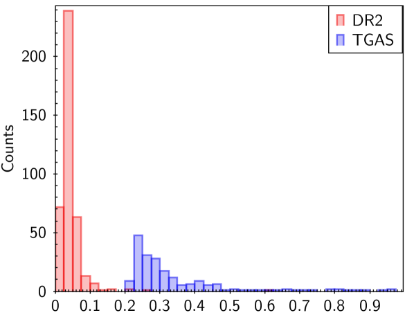
Figure 1: Distribution of the DR2 parallax uncertainties for our sample of 401 RRLs (red histogram) and the TGAS parallax uncertainties for the subsample of 199 RRLs for which TGAS parallaxes were published in Gaia DR1 (blue histogram). The bin size is 0.025 mas.

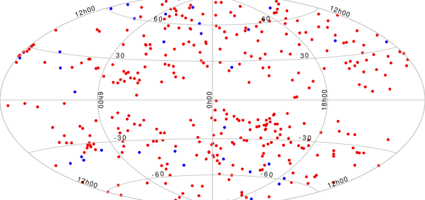
Figure 2: Sky distribution of our sample of 401 RRLs in Galactic coordinates. Red and blue filled circles show RRab and RRc stars respectively.

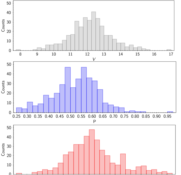
Figure 3: Distribution in apparent $V$ mean magnitude (upper panel), period (middle panel) and metallicity (on the Zinn & West 1984 metallicity scale; lower panel) for the RRLs in our sample. $V$ mean magnitudes are available for 382 RRLs in our sample of 401 variables, metallicities for 400 RRLs, while pulsation periods are available for the whole sample of 401 stars.

A weighted least-squares fit of the relation $\varpi_{TGAS}=\alpha\varpi_{DR2}$ returns a slope $\alpha=1.02\pm 0.02$, which is close to the bisector line slope. However, there is a significant spread for $\varpi_{DR2}\sim 0.3-1$ mas in Fig. 4, with the TGAS parallaxes having negative or significantly larger values than the DR2 parallaxes. The non-weighted mean difference between DR2 and TGAS parallaxes: $\Delta\varpi_{0}=\varpi_{\rm DR2}-\varpi_{\rm TGAS}$, omitting RR Lyr itself, is $-0.04$ mas. However, the large uncertainties of the TGAS parallaxes prevent a reliable estimation of any zero-point offset that might exist between the DR2 and the TGAS parallaxes of RRLs.

Table 2 shows the comparison for five RRLs for which Hipparcos, HST, TGAS and Gaia DR2 parallax measurements are available. There is a general agreement between the HST, TGAS and DR2 parallaxes except for RR Lyr. Fig. 5 shows the Hipparcos (lower panel), HST (middle panel) and TGAS (upper panel) parallaxes plotted versus Gaia DR2 parallaxes for 4 of those five RRLs. For the sake of clarity we did not plot RR Lyr in the figure. Similarly to Fig. 4 the upper panel of Fig. 5 shows the nice agreement existing between TGAS and DR2 parallaxes. Agreement between Gaia DR2 and Hipparcos parallaxes (lower panel) is less pronounced; on the contrary, a very nice agreement of the DR2 and HST parallaxes is seen in the middle panel of Fig. 5, confirming the reliability of the Gaia DR2 parallaxes. However, the sample of RRLs with both, DR2 and HST parallax estimates available is too small to measure any possible zero-point offset of the Gaia parallaxes with respect to HST. The interested reader is referred to Arenou et al. (2018) who validated Gaia DR2 catalogue and found a negligible ($-0.01\pm 0.02$ mas) offset between the HST and DR2 parallaxes using a sample of stars significantly larger than the few RRLs that could be used here.

Table 2: Hipparcos, HST, TGAS and Gaia DR2 parallaxes of RRLs for which these independent measurements are available.

Name	$\varpi_{Hipparcos}$	$\varpi_{HST}$	$\varpi_{\rm TGAS}$	$\varpi_{\rm DR2}$
	(mas)	(mas)	(mas)	(mas)
RR Lyr	$3.46\pm 0.64$	$3.77\pm 0.13$	$3.64\pm 0.23$	$-2.61\pm 0.61$
RZ Cep	$0.59\pm 1.48$	$2.12\pm 0.16*$	$2.65\pm 0.24$	$2.36\pm 0.03$
SU Dra	$0.20\pm 1.13$	$1.42\pm 0.16$	$1.43\pm 0.28$	$1.40\pm 0.03$
UV Oct	$2.44\pm 0.81$	$1.71\pm 0.10$	$2.02\pm 0.22$	$1.89\pm 0.03$
XZ Cyg	$2.29\pm 0.84$	$1.67\pm 0.17$	$1.56\pm 0.23$	$1.57\pm 0.03$

* Benedict et al. (2011) provide two values for the parallax of RZ Cep: $\varpi=2.12$ mas and $\varpi=2.54$ mas, with the former being the final and preferred adopted value (according to Benedict private communication in Monson et al. 2017).

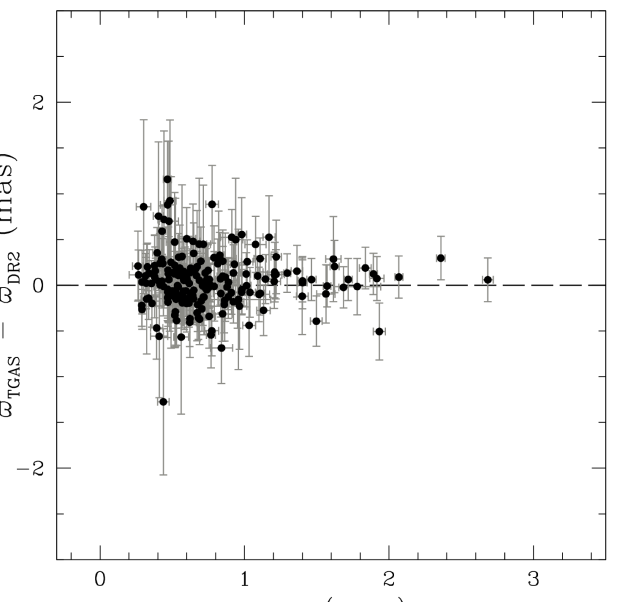
Figure 4: Comparison of the TGAS and DR2 parallaxes for 198 RRLs for which both parallax estimates are available. For clarity, RR Lyr was omitted (see text for details).

Figure 5: Comparison of the DR2 and TGAS (upper panel), DR2 and HST (middle panel), and DR2 and Hipparcos (lower panel) parallaxes for RRLs studied by Benedict et al. (2011) with the HST (see also Table 2). RR Lyr was omitted (see text for the details). The solid lines represent the bisectors.

3.2 Comparison of the $PL$ relations

Gaia Collaboration et al. (2017) in their figure 23 show the impressive improvement of $PM_{K_{\rm s}}$ relation of RRLs when going from the Hipparcos to the TGAS parallaxes. In this section we extend the comparison to the DR2 parallaxes. To transform the trigonometric parallaxes to absolute magnitudes we used the canonical relation:

$$M=m_{0}+5\log\varpi-10,$$ (1)

that links the star absolute magnitude $M$ and its de-reddened apparent magnitude $m_{0}$ to the star parallax in mas: $\varpi$. Eq. 1 holds only for true (hence with formally zero or negligible uncertainties) absolute magnitudes, apparent magnitudes and parallaxes. However, the direct transformation of parallaxes to the absolute magnitudes adopting Eq. 1 cannot be used for measured values that have non negligible uncertainties (Gaia Collaboration et al. 2017, Luri et al. 2018). This is because the direct inversion of the measured parallaxes to estimate the distance is well behaved in the limit of negligible uncertainties, but degrades quickly as the fractional uncertainty of the parallax grows, resulting in estimates with large biases and variances. Furthermore, negative parallaxes cannot be transformed into absolute magnitudes, thus an additional sample selection bias is introduced, since objects with the negative parallaxes must be removed from the sample. The Bayesian fitting approach we apply in the present study allows us to avoid these issues as it is fully discussed in Section 4. However, only for visualisation purposes in this section we transformed the Hipparcos, TGAS and DR2 parallaxes in the corresponding absolute $M_{K_{\rm s}}$ magnitudes using Eq. 1. This transformation is possible only for 394, 195 and 96 RRLs in our sample, for which positive parallaxes in the DR2, TGAS and Hipparcos catalogues, respectively, are available. The corresponding $PM_{K_{\rm s}}$ distributions are shown in Fig. 6, that were obtained by correcting the apparent $K_{\rm s}$ mean magnitudes for extinction and after “fundamentalizing" the RRc stars by adding 0.127 to the logarithm of the period. The $PM_{K_{\rm s}}$ distribution in the upper panel of Fig. 6 shows the improvement of the DR2 parallaxes with respect to the TGAS (middle panel) and Hipparcos (lower panel) measurements. To guide the eye we plot as blue lines the $PM_{K}$ relation provided in eq. 14 by Muraveva et al. (2015):

$$M_{K}=-2.53\log(P)-0.95.$$ (2)

The bottom panel of Fig. 6 shows that the 96 RRLs with Hipparcos parallaxes are systematically shifted towards fainter absolute magnitudes. This is because by removing sources with negative parallaxes we are removing, preferentially, RRLs at larger distances, of which Hipparcos could measure only the brightest. Those distant bright RRLs typically will have small true parallaxes, close to zero or even negative, owing to the larger uncertainties particularly in Hipparcos. Hence, the net effect of removing RRLs with negative parallaxes in the Hipparcos sample is to bias the remaining sample towards fainter absolute magnitudes as it is clearly seen in the bottom panel of Fig. 6.

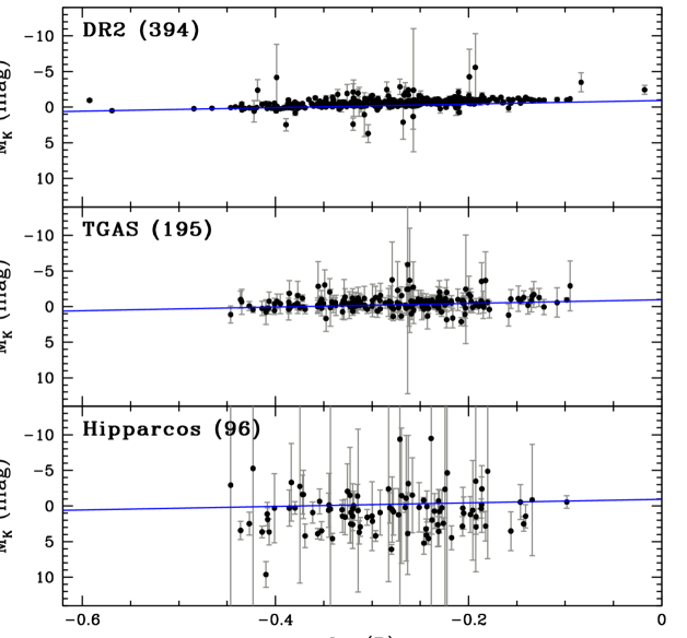
Figure 6: RRL $PM_{K_{\rm s}}$ distributions obtained inferring the absolute magnitudes in the $K_{\rm s}$-band by direct transformation of the Gaia DR2 (upper panel), TGAS (middle panel) and Hipparcos (lower panel) parallaxes using Eq. 1. Blue lines represent the $PM_{K}$ relation (eq. 14 from Muraveva et al. 2015). The period is measured in days.

3.3 Comparison with Baade-Wesselink studies

Figure 7: Comparison of the photometric parallaxes inferred from $M_{V}$ (upper panel) and $M_{K}$ (bottom panel) absolute magnitudes estimated via BW method and the corresponding DR2 parallaxes for 23 MW RRLs for which both parallax estimates are available. The solid lines represent the bisectors.

In this section we compare the DR2 trigonometric parallaxes with photometric parallaxes inferred from the Baade-Wesselink (BW) technique, which are available for some of the RRLs in our sample. Muraveva et al. (2015) summarise in their table 2 the absolute visual ($M_{V}$) and $K$-band ($M_{K}$) magnitudes obtained from the BW studies (Cacciari et al. 1992, Skillen et al. 1993, Fernley et al. 1998 and references therein) for 23 MW RRLs. The BW absolute magnitudes were revised assuming the value 1.38 (Fernley, 1994) for the p factor used to transform the observed radial velocity to true pulsation velocity and averaging multiple determinations for individual stars. All 23 RRL variables with absolute magnitudes estimated via BW technique have a counterpart in our sample of 401 RRLs. The comparison of the photometric parallaxes inferred from the BW $M_{V}$ and $M_{K}$ absolute magnitudes and the corresponding Gaia DR2 parallaxes for these 23 RRLs is shown in the upper and bottom panels of Fig.7, respectively. A weighted least squares fit of the relations $\varpi_{M_{V(BW)}}=\alpha\varpi_{\rm DR2}$ and $\varpi_{M_{K(BW)}}=\alpha\varpi_{\rm DR2}$ returns the same slope value of 1.06, which is close to the bisector slope $\alpha=1$. Even though the DR2 parallaxes of these 23 RRLs are generally in good agreement with the photometric parallaxes obtained in the BW studies, we notice that there is a systematic difference between the two sets of parallaxes. Specifically, the mean non-weighted differences $\Delta\varpi_{0}=\varpi_{\rm DR2}-\varpi_{M_{V(BW)}}$ and $\Delta\varpi_{0}=\varpi_{\rm DR2}-\varpi_{M_{K(BW)}}$ are both equal to $-0.07$ mas. That is, the Gaia DR2 parallaxes for these 23 RRLs seem to be generally smaller than the photometric parallaxes inferred from the BW studies. However, in the parallax offset estimate we used the direct transformation of the absolute magnitudes to parallaxes and assumed symmetric Gaussian uncertainties for the sake of simplicity. Moreover, this offset is based on a relatively small number of close stars and depends on the specific value adopted for the p factor. We perform a more careful analysis of the potential Gaia DR2 parallax offset for RRLs and further discuss this topic in Section 5.2.

4 Method

4.1 Description of the Bayesian approach

In Delgado et al. (2018) we presented a Bayesian hierarchical method to infer the $PM$ and $PMZ$ relationships. The hierarchical models were validated with semi-synthetic data and applied to the sample of 200 RRLs described in Gaia Collaboration et al. (2017). Simplified versions of these models were also used in Gaia Collaboration et al. (2017). A full description of these models is beyond the scope of this manuscript and we recommend the interested reader to consult Delgado et al. (2018) for a more in-depth description of them. In what follows, we summarize what we consider are the minimum details about the hierarchical Bayesian methodology and our models necessary to understand the present paper as a self-contained study.

The core of the hierarchical Bayesian methodology consists of partitioning the parameter space associated to the problem into several hierarchical levels of statistical variability. Once this partition is done, the modelling process assigns probabilistic conditional dependency relationships between parameters at the same or different levels of the hierarchy. The construction of the model is finished when one is able to express a joint probability function of all the parameters of the model which factorizes as a product of conditional probability distributions. This factorization defines a Bayesian network (Pearl, 1988; Lauritzen, 1996) consisting of a Directed Acyclic Graph (DAG) in which nodes encode model parameters and directed links represent conditional probability dependence relationships.

All models presented in Delgado et al. (2018) have three-level hierarchies. In all of them we partition the parameter space into measurements ($\mathcal{D}$), true astrophysical parameters ($\Theta$) and hyperparameters ($\Phi$). In this case, the joint probability distribution associated to our models is given by

$$p\left(\mathcal{D},\mathbf{\Theta},\Phi\right)=p\left(\mathcal{D}\mid\mathbf{\Theta}\right)\cdot p\left(\mathbf{\Theta}\mid\Phi\right)\cdot p\left(\Phi\right)\,,$$ (3)

where $p\left(\mathcal{D}\mid\Theta\right)$ is the conditional distribution of the data given the parameters (the so called likelihood), $p\left(\mathbf{\Theta}\mid\Phi\right)$ is the prior distribution of the true parameters given the hyperparameters and $p\left(\Phi\right)$ is the unconditional hyperprior distribution of the hyperparameters. Bayesian inference is based on Bayes’ rule:

$$p\left(\mathbf{\Theta},\Phi\mid\mathcal{D}\right)\propto p\left(\mathcal{D}\mid\mathbf{\Theta}\right)\cdot p\left(\mathbf{\Theta}\mid\Phi\right)\cdot p\left(\Phi\right)\,,$$ (4)

and its goal is to infer the marginal posterior distribution $p\left(\Lambda\mid\mathcal{D}\right)$ of some subset [$\Lambda\subseteq\left(\mathbf{\Theta},\Phi\right)$] of the parameters of interest. For the statistical inference problem of calibrating the RRL fundamental relationships, in this paper we primarily focus on inferring the parameters of such relationships. However, we also aim at getting insight on the true posterior distribution of Gaia DR2 parallaxes given their measured values.

In Figure 8 we present the generic DAG that encodes the probabilistic relationships between the parameters of all the models applied in this paper. The graph is intended to represent several models at once. For example, for a model devoted to infer a $PM$ relation, the nodes depicted with dimmer colours and their corresponding arcs do not belong to the model and the reader should not consider them.

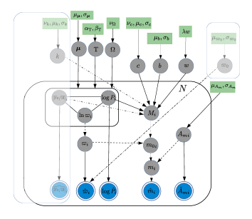
Figure 8: Directed Acyclic Graph (DAG) that represents the generic Hierarchical Bayesian Method (HBM) used to infer the coefficients of the $PM$, $PMZ$ and optical absolute magnitude-metallicity ($MZ$) relations.

The DAG of Fig. 8 shows the measurements at the bottom level as blue nodes: decadic logarithm of periods $\log\hat{P}_{i}$, apparent magnitudes $\hat{m}_{i}$, metallicities $\widehat{\left[\mathrm{Fe/H}\right]}_{i}$, parallaxes $\hat{\varpi}_{i}$ and extinctions $\hat{A}_{m_{i}}$ The subindex $i$ runs from 1 to the total number of stars $N$ in the sample. For each measurement there is a corresponding true value in the DAG. True values are represented as measurements but without the circumflex accent (^) and are depicted by grey nodes. The model assumes that all measurements are realizations from normal distributions centred at the true (unknown) values and with standard deviations given by the measurement uncertainties provided by each catalogue. Note that true values and measurements are enclosed in a black rectangle that represents sample replication for $i=1,2,...,N$ (plate notation). The model also takes into account the effect of the interstellar absorption when generating the measured apparent magnitudes from the true ones. So, it distinguishes between true (unabsorbed) apparent magnitudes ${m_{0}}_{i}$ and true (absorbed) apparent magnitudes $m_{i}$ and deterministically computes the latter ones as $m_{i}={m_{0}}_{i}+A_{m_{i}}$, where ${A_{m}}_{i}$ represents the true absorption. This deterministic dependency of absorbed on unabsorbed apparent magnitude and true extinction is represented by dashed arrows in the DAG.

Once we have explained how the model manages the interstellar absorption, we describe how it generates the true (unabsorbed) apparent magnitudes ${m_{0}}_{i}$ from true parallaxes $\varpi_{i}$ and absolute magnitudes $M_{i}$. This is done by means of the deterministic relationship, coming from Eq. 1:

$${m_{0}}_{i}=M_{i}-5\log(\varpi_{i})+10\,,$$ (5)

which is represented in the DAG by the dashed arcs going from $\varpi_{i}$ and $M_{i}$ to ${m_{0}}_{i}$. The model also contemplates the existence of a Gaia global parallax offset $\varpi_{0}$ as suggested by Arenou et al. (2018). This offset can be inferred by the model itself or fixed to a predefined value.

The central core of the model is the submodel for the $PMZ$ relation in which absolute magnitudes $M_{i}$ are parameterized by

$$M_{i}\sim\mathsf{t}_{5}\left(b+c\cdot\log P_{i}+k\cdot\left[\mathrm{Fe/H}\right]_{i},w\right)\,,$$ (6)

where $\sim$ should be read as ‘is distributed as’ and $\mathsf{t}_{5}$ represents a Student’s t distribution with five degrees of freedom. The mean of this distribution is a linear model in three parameters: the intercept $b$, the slope $c$ for the period term (in decadic logarithmic scale), and the slope $k$ for the metallicity term, and its scale $w$ represents the linear model intrinsic dispersion. This intrinsic dispersion aims at including all potential effects not accounted for explicitly in the model (e.g. evolutionary effects). The dependency of absolute magnitude on the linear model parameters, intrinsic dispersion and predictive variables is represented in the DAG by all the incoming arrows to the node $M_{i}$. A Student’s t distribution was chosen in order to make the model robust against outliers such as RR Lyr itself and a few other stars with potentially problematic DR2 parallax and parallax uncertainty values.

For the slopes $c$ and $k$ of the $PMZ$ relationship of Eq. 6 we specify weakly informative Student’s t-priors with location parameter $\mu_{c}=\mu_{k}=0$, and for the intercept we use a vague Gaussian prior centred at $\mu_{b}=0$. The intrinsic dispersion of the $PMZ$ relation is given an exponential prior with inverse scale $\lambda_{w}=1$. We use green rectangular nodes at the top of the graph to denote all these fixed prior hyperparameters.

In Delgado et al. (2018) we reported the existence of a systematic correlation between measured periods, metallicities and parallaxes in our sample. This correlation occurred in the sense that a slight decrease of the median period calculated in bins of parallax corresponds to an increase of the median parallax and the median metallicity. We also demonstrated that without a proper modelling of this systematic effect the inference carried out with the TGAS parallax measurements returned a severely underestimated slope in $\log(P)$ of the $PMZ$ relation. We also showed that for the typical DR2 parallax uncertainties, the impact of the underestimation is severely reduced. In any case, our model assigns a joint prior to the true values of $\log P_{i}$ and $\varpi_{i}$ in order to prevent this bias. This prior is defined as

$$\left(\log P_{i},\ln\varpi_{i}\right)\sim\mathsf{MN}\left(\bm{\mu},\mathrm{T}\Omega\mathrm{T}\right)\,,$$ (7)

where $\mathsf{MN}$ represents a 2D Gaussian distribution with mean vector $\bm{\mu}=(\mu_{P},\mu_{\omega})$, diagonal matrix of standard deviations $\mathrm{T}=\mathrm{diag}(\sigma_{P},\sigma_{\omega})$ and correlation matrix $\Omega$. We parametrize each component of the mean vector $\bm{\mu}$ by a weakly informative Gaussian prior centred at 0 and with standard deviation $\mathrm{\sigma}_{\bm{\mu}}=5$. For each standard deviation in $\mathrm{T}$ we assign a weakly informative Gamma distribution prior with shape $\alpha_{\mathrm{T}}=0.1$ and inverse scale $\beta_{\mathrm{T}}=0.1$. For the correlation matrix $\Omega$ we specify a LKJ prior (Lewandowski et al., 2009) with $\nu_{\Omega}=1$ degrees of freedom. To every true value of ${\left[\mathrm{Fe/H}\right]}_{i}$ our model assigns a non-informative Gaussian prior which reflects our limited knowledge about the true distribution of metallicities, given the heterogeneous provenance of metallicities in Dambis et al. (2013) sample.

5 Characteristic relations for RRLs

5.1 $M_{V}-{\rm[Fe/H]}$ relation

A vast and long-standing literature exists on the visual $M_{V}-{\rm[Fe/H]}$ relation of RRLs (see e.g. Clementini et al. 2003; Cacciari & Clementini 2003; Dambis et al. 2013 and references therein). The relation is generally assumed to have a linear form: $M_{V}=\alpha[Fe/H]+\beta$, with literature values for the slope $\alpha$ of the metallicity term ranging from $0.30-0.37$ (Sandage, 1993; Feast, 1997) to 0.13 (Fusi Pecci et al., 1996) and an often adopted mild slope of $\alpha=0.214\pm 0.047$ mag/dex, as estimated from a photometric and spectroscopic study of about a hundred RRLs in the bar of the LMC (Clementini et al. 2003; Gratton et al. 2004). Those studies also showed the $M_{V}-{\rm[Fe/H]}$ relation to be, in first approximation, linear and universal. On the other hand, theoretical studies (e.g. Caputo et al. 2000b; Bono et al. 2003; Catelan et al. 2004) suggest that the $M_{V}-{\rm[Fe/H]}$ relation is not linear over the whole metallicity range spanned by the MW RRLs (almost 3 dex for MW field variables). Indeed, theoretical studies (e.g. Caputo et al. 2000b; Bono et al. 2003) state that $\alpha$ presents a relatively mild value of $0.17\pm 0.069$ mag/dex for RRLs with ${\rm[Fe/H]}\leq-1.6$ dex and becomes significantly steaper, $0.359\pm 0.027$ mag/dex, for RRLs with ${\rm[Fe/H]}>-1.6$ dex.

In this paper we study the $M_{V}-{\rm[Fe/H]}$ relation of RRLs applying the Bayesian approach described in Section 4 to 381 RRLs, out of our sample of 401, for which all needed information (apparent $V$ mean magnitudes, extinction, metal abundances) are available from Dambis et al. (2013) and trigonometric parallaxes are available in Gaia DR2. Slope, zero-point and intrinsic dispersion obtained for the $M_{V}-{\rm[Fe/H]}$ relation with our approach are summarised in the first row of Table 3. The metallicity slope we obtain, $\alpha=0.40\pm 0.03$ mag/dex, implies a much stronger dependence of the RRL absolute $V$ magnitude on metallicity than ever reported previously in the literature. In Section 5.2 we argue that this steep slope may be due to an offset affecting the DR2 parallaxes. However, we first check here whether the high metallicity dependence is not caused by a flaw in our Bayesian procedure.

Table 3: $M_{V}-{\rm[Fe/H]}$ relation of RRLs in linear form obtained with our Bayesian approach when a Gaia DR2 parallax zero-point offset, $\Delta\varpi_{0}$, is fixed in the model: (1) number of stars used in the fit; (2) and (3) slope and zero-point of the relation; (4) intrinsic dispersion; (5) adopted value for the Gaia DR2 parallax zero-point offset.

	No. stars	$\alpha$	$\beta$	$w$	$\Delta\varpi_{0}$
	$381$	${0.40}_{-0.03}^{+0.03}$	${1.01}_{-0.04}^{+0.04}$	${0.17}_{-0.01}^{+0.01}$	$0.00$
	$381$	${0.37}_{-0.03}^{+0.03}$	${1.09}_{-0.04}^{+0.04}$	${0.15}_{-0.01}^{+0.01}$	$-0.03$
	$381$	${0.33}_{-0.02}^{+0.03}$	${1.19}_{-0.04}^{+0.04}$	${0.15}_{-0.01}^{+0.01}$	$-0.07$
	$23$	${0.27}_{-0.06}^{+0.06}$	${0.94}_{-0.08}^{+0.08}$	${0.14}_{-0.03}^{+0.04}$	$0.00$
	$23$	${0.27}_{-0.06}^{+0.05}$	${0.99}_{-0.08}^{+0.08}$	${0.13}_{-0.03}^{+0.04}$	$-0.03$
	$23$	${0.26}_{-0.05}^{+0.05}$	${1.06}_{-0.07}^{+0.07}$	${0.13}_{-0.03}^{+0.04}$	$-0.07$

To this end we carried out simulations with semi-synthetic data. The semi-synthetic data were created according to the following recipe:

• we generated true metallicities drawn from Gaussian distributions (one for each star) centred at the measured values and with standard deviations given by the uncertainties described in Section 2;

• absolute magnitudes $M_{V}$ were derived from the true metallicities generated above using the $M_{V}-{\rm[Fe/H]}$ relationship by Federici et al. (2012): $M_{V}=0.25{\rm[Fe/H]}+0.89$;

• true de-reddened apparent magnitudes were generated from Gaussian distributions centred at the observed values and with standard deviations given by the measurement uncertainties corrected for $V$-band extinctions generated likewise centred at the values in Dambis et al. (2013);

• finally, the true parallaxes were derived from the true absolute and apparent magnitudes, and the measured parallaxes were drawn from Gaussian distributions centred at the true values with standard deviations given by the Gaia DR2 parallax uncertainty of each star.

Our aim is to evaluate the capability of our methodology to recover unbiased estimates of the true parameters, in particular of the relationship slope. We infer posterior distributions of the model parameters for 10 realisations of the semi-synthetic data. The inferred slopes range between 0.238 and 0.274 mag/dex with a mean of 0.259 mag/dex (the true value used in the generation of the data being 0.25) with a constant credible interval of $\pm 0.05$. This represents a mild overestimation of the true slope which could be due to the imperfection of the assumed priors and the relatively small number of simulations. We have also applied models with a prior for the parallax that is independent of the period. As discussed in Delgado et al. (2018), this neglects the existence of a correlation between parallax and period in our sample and, as expected, results in slopes that are systematically biased (yielding an average slope from 10 random realisations of the semi-synthetic data set of 0.31 mag/dex and a posterior standard deviation of 0.05). In summary, we find that the Bayesian model designed and applied to the data is not the cause for the slopes being higher than expected according to the previous studies.

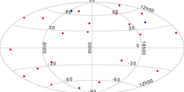
Figure 9: Sky distribution in Galactic coordinates of 23 RRLs for which absolute magnitudes in the $V$ and $K$ bands have been estimated using the BW technique. Red and blue filled circles show RRab and RRc stars, respectively.

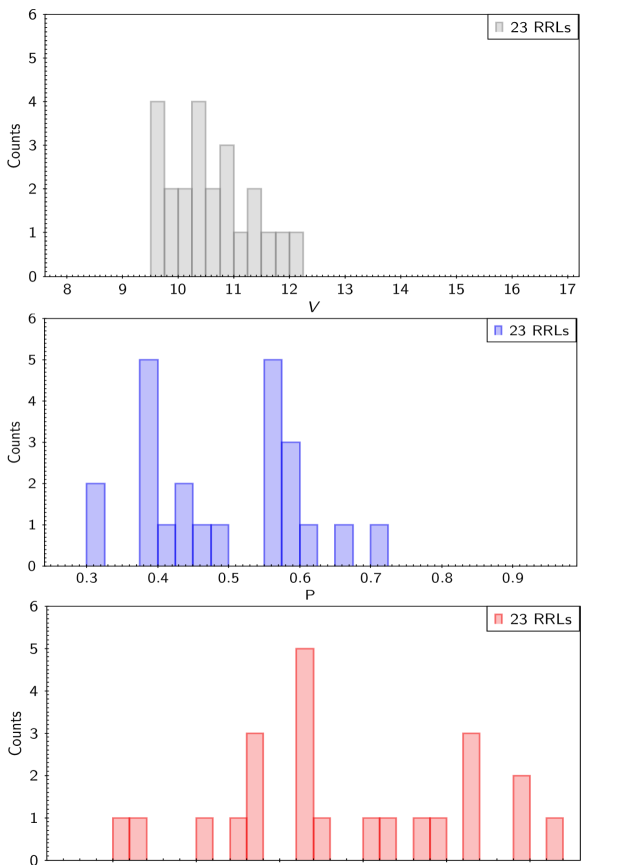
Figure 10: Distribution in apparent $V$ magnitude (upper panel), period (middle panel) and metallicity (as derived from high-resolution spectroscopy; lower panel) for the 23 RRLs in Fig. 9.

The steeper slope found by our methodology can be compared with alternative inference methods commonly used in the literature. We can compare the results with the weighted least-squares estimate when the weights are inversely proportional to the uncertainties in both the predicting and predicted variables. We interpret that this is the methodology applied when it is claimed in the literature that the fit was a weighted linear least-squares model with uncertainties in both axes. Details about how uncertainties are combined are often missing in the literature. We will assume that a simple quadratic addition was put in place. However, this is far from optimal as it does not include a full forward model of how the data were created and does not distinguish between uncertainties in absolute magnitude and metallicity. The effects of uncertainties in each of the axes are significantly different in size and nature, hence we only include these results for the sake of comparison. If we apply this weighted least-squares approximation to the absolute magnitudes naively computed by parallax inversion (Eq. 1), as a consequence, truncating the sample by removing negative parallaxes, we obtain a slope value of $\alpha=0.36\pm 0.03$. Therefore, it seems there is evidence for a steeper slope even from the less sophisticated method that does not include intrinsic dispersion, does not deal correctly with the uncertainties in the absolute magnitude and truncates the sample. We conclude that the high metallicity slope of the $M_{V}-{\rm[Fe/H]}$ relation is not caused by the selected inference method, and rather reflects the real distribution of the data. In this case, selecting a sample with accurately homogenised metallicity estimates becomes crucially important. Metallicity estimates used for our study are provided by Dambis et al. (2013), who in their turn compiled metal abundances obtained in a number of different studies and include metallicity values inferred from the Fourier analysis of the RRLs light curves or using high- or low-resolution spectroscopy. For the sake of homogeneity Dambis et al. (2013) transformed the estimated metallicity values to the unique Zinn & West (1984) metallicity scale. This transformation could cause an additional bias which is hard to account for. Furthermore, uncertainties in metallicities were not provided by Dambis et al. (2013), hence, we assigned approximate values of uncertainties (see Section 2), that could also affect the results of our fit. In order to avoid all these issues we decided to use a sample of 23 MW RRLs studied by Muraveva et al. (2015), for which homogeneous metallicities and related uncertainties based on abundance analysis of high-resolution spectroscopy (Clementini et al. 1995, Lambert et al. 1996) are available. All 23 RRLs have counterparts in our sample of 401 RRLs. Their distribution on the sky is shown in Fig. 9. Their apparent $V$ magnitudes and periods expectably span narrower ranges than the full sample of 401 RRLs, namely, from 9.55 to 12.04 mag in apparent visual mean magnitude and from 0.31 to 0.71 days in period. Metal abundances for these 23 RRLs are in the range from $-2.5$ to +0.17 dex, which is comparable with the range of metallicities spanned by our 401 RRL full sample (see Section 2). The distributions in $V$ magnitude, period and metallicity of the 23 RRLs are shown in Fig. 10, where for ease of comparison we use the same scales for the abscissa axes as in Fig. 3. Slope, zero-point and dispersion of the RRL $M_{V}-{\rm[Fe/H]}$ relation obtained by applying our Bayesian approach to the sample of 23 RRLs are summarised in the first row of the lower portion of Table 3. The metallicity slope ($\alpha=0.27\pm 0.06$) is shallower than obtained from the whole sample of 381 RRLs, that may be the effect of using more accurate and homogeneous spectroscopic metallicities, and yet is still steeper than found in the more recent literature, even though (marginal) agreement exists within the uncertainties. A clue to further investigate the metallicity dependence issue may be to study the $M_{V}-{\rm[Fe/H]}$ relation defined by large samples of RRLs in globular clusters for which the metallicity is well known from high resolution spectroscopic studies. This is addressed in a following paper (Garofalo et al., in preparation). Meanwhile, in Section 5.2 we examine whether the existence of a zero-point offset in the Gaia DR2 parallaxes (Arenou et al. 2018) might contribute to produce the high slope we find for the RRL $M_{V}-{\rm[Fe/H]}$ relation.

5.2 Gaia DR2 parallax offset

The Gaia DR2 parallaxes are known to be affected by an overall zero-point whose extent varies depending on the sample used to infer its value and, typically, is of the order of $-0.03$ mas, as inferred by comparison with QSO parallaxes (Arenou et al. 2018). After Gaia DR2 a number of studies have appeared in the literature (Riess et al. 2018; Zinn et al. 2018; Stassun & Torres 2018) all suggesting that Gaia provides smaller parallaxes, hence, larger distance estimates, than derived from other independent techniques, that is, $\Delta\varpi_{0}=\varpi_{\rm DR2}-\varpi_{indep.}$ is negative, but by how much varies from one study to the other. For instance, Riess et al. (2018) estimated a zero-point offset for Gaia DR2 parallaxes of $-0.046$ mas, combining HST photometry and Gaia DR2 parallaxes for a sample of 50 Cepheids. In the paper describing the final validation of all data products published in Gaia DR2, Arenou et al. (2018) estimate an offset $\Delta\varpi_{0}=-0.056\pm 0.005$ mas for RRLs in the Gaia DR2 catalogue and $-0.033\pm 0.009$ mas for a sample of RRLs in the GCVS. In the following we investigate whether the zero-point offset of the Gaia DR2 parallaxes for RRLs can affect the slope and zero-point inferred for their $M_{V}-{\rm[Fe/H]}$ relation. We remind the reader that the non-linear relationship between parallax and absolute magnitude (Eq. 1) implies that a given parallax offset does not affect all absolute magnitudes equally. Just for illustration purposes, a parallax offset of $-0.056$ mas as suggested by Arenou et al. (2018) for the RRLs would result in a change of the distance modulus equal to 0.2 mag at 1 kpc, while at 7 kpc it would amount to 1.1 mag. We are located in a relatively metal-rich area of the MW, while farther RRLs in our sample belong to the halo and likely are more metal-poor. Thus, the negative zero-point offset in the DR2 parallaxes will make farther/metal-poor RRLs to appear intrinsically brighter, hence causing an overestimation of the $M_{V}-{\rm[Fe/H]}$ relation slope. Therefore, our discussion of the results must incorporate the effect of potential parallax offsets. The upper portion of Table 3 lists inference results for a series of linear $M_{V}-{\rm[Fe/H]}$ models characterised by different parallax offsets, namely, models without offset, with a global offset of $-0.03$ mas (Arenou et al. 2018) and with an offset of $-0.07$ mas, as suggested by the comparison with the absolute magnitudes derived from the BW studies (Section 3.3) and used here only for demonstration reasons. Results of this test show that it is of crucial importance to take into account a potential parallax offset when studying the RRL $M_{V}-{\rm[Fe/H]}$ relation because the slope of the relation varies with the offset and decreases systematically with increasing the value adopted for the parallax offset, from $\alpha=0.40$ (no offset), to $\alpha=0.33$ for an offset of $-0.07$ mas. We applied the same model to the 23 MW RRLs with homogeneous metallicity estimates based on abundance analysis of high-resolution spectra (see Section 5.1), assuming no parallax offset and the offsets of $-0.03$ mas and $-0.07$ mas. The resulting relations are shown in the lower portion of Table 3. The slope of the $M_{V}-{\rm[Fe/H]}$ relation varies from $0.27$ (no offset) to $0.26$ (offset of $-0.07$ mas), showing that for the sample of 23 RRLs, which have both distances and range of distances much smaller than for the full sample, the impact of a potential parallax offset on the slope of the $M_{V}-{\rm[Fe/H]}$ relation is greatly reduced.

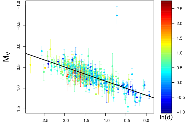
Figure 11: $M_{V}-{\rm[Fe/H]}$ relation defined by the 381 RRLs in our sample, whose absolute $M_{V}$ magnitudes were inferred from the model described in Section 4. The solid line represents the linear fit. Its slope and zero-point are summarised in the first portion of Table 4 (first row). The colour scale encodes the (natural) logarithm of the inferred (true) distance measured in units of kpc.

To compute all the relationships presented in this paper we use the model that includes the potential parallax offset as a parameter (Section 4). We fitted the $M_{V}-{\rm[Fe/H]}$ relation defined by the whole sample of RRLs inferring simultaneously the relation parameters (slope and zero-point) and the parallax offset. Corresponding results are summarised in the first panel of Table 4 (first row). From our sample of 381 RRLs we obtain a mean posterior metallicity slope of 0.34 for a mean posterior offset of $-0.062$ mas. The resulting $M_{V}-{\rm[Fe/H]}$ fit is shown in Fig. 11, where colours encode the (natural) logarithm of the inferred distance.

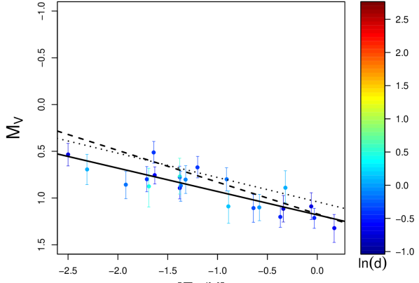
Figure 12: $M_{V}-{\rm[Fe/H]}$ relation defined by the 23 RRLs with metallicity from high resolution spectroscopy, whose absolute $M_{V}$ magnitudes were inferred from the model described in Section 4. The solid line represents the linear fit. Its slope and zero-point are summarised in the second portion of Table 4. For comparison, the dashed line represents the relationship inferred from the $381$ RRLs shown in the first portion of the same Table. The dotted line represents the relationship inferred by a model for the 23 RRLs with a parallax offset fixed to $-0.057$ mas and shown in the third portion of Table 4. The colour scale encodes the (natural) logarithm of the inferred (true) distance measured in units of kpc.

We applied the same model to the 23 MW RRLs with homogeneous metallicity estimates. The resulting $M_{V}-{\rm[Fe/H]}$ relation is shown in the second panel of Table 4. In the case of the 23 MW RRLs, the reduced number of sources and the smaller range of distances (visible from the colour scale in Fig. 12) do not constrain the value of the offset. The first row of the second portion of Table 4 summarises the posterior distribution for the offset with a mean of $-0.142^{+0.06}_{-0.06}$ which seems implausible. This translates directly into a much smaller metallicity slope of 0.25 $\pm$ 0.05 mag/dex compared to the one inferred for the 381 stars sample. If we remove the determination of the parallax offset as a parameter of the model and, instead, adopt a constant value for the offset of $-0.057$ mas, which corresponds to the average of the offsets obtained from fitting the linear $M_{V}-{\rm[Fe/H]}$ relation ($-$0.062 mas; Section 5.1), and the $PM_{K}Z$, $PM_{W1}Z$ relations ($-$0.054 and $-$0.056 mas, respectively; Section 5.3) to the full sample of RRLs, we obtain a slope of $0.26\pm 0.05$ for the sample of 23 RRLs. The resulting $M_{V}-{\rm[Fe/H]}$ relation is shown in the third portion of Table 4.

To conclude even though using the reduced sample of 23 RRLs has the advantage of (i) a smaller effect of the parallax offset as the 23 RRLs are nearby stars; (ii) a more accurate estimation of metallicity based on high-resolution spectroscopy, we must stress that selection effects can potentially be stronger, as only nearby bright RRLs are characterised by high enough signal-to-noise ratios to be analysed with high-resolution spectroscopy, hence, biasing the results.

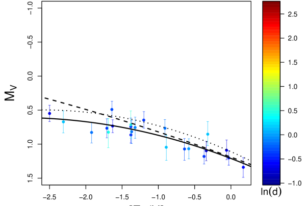
Figure 14: Same as in Fig. 12 but with lines representing the quadratic $M_{V}-{\rm[Fe/H]}$ relations.

Since a number of theoretical studies suggest a non-linear $M_{V}-{\rm[Fe/H]}$ relation, we have also explored quadratic relationships between $M_{V}$ and $\rm[Fe/H]$. Table 4 includes a summary of the posterior distributions of selected model parameters. In the two cases (381 and 23 RRL samples), the effect of including a second order term is to increase the mean value of the first order term posterior distribution from 0.34 to 0.39 (sample of 381 stars) and from 0.25 to 0.41 (sample of 23 stars). We mentioned above that there is a controversy relative to the nature (linear or quadratic) of the relationship between metallicity and absolute magnitudes. We have therefore attempted to assess the relative merit of the two models (linear and quadratic) in the light of the available data. In doing so, we are limited by the sampling scheme chosen (Hamiltonian MonteCarlo as implemented in Stan; Carpenter et al., 2017). Given this implementation, we cannot use evidences or Bayes’ factors and resort to the Bayesian leave-one-out estimate of the expected log-pointwise predictive density (Vehtari, Gelman & Gabry, 2017). The comparison of the values obtained for the two models is inconclusive: the mean value of the paired differences is $-4.4\pm 8.8$ favouring the more complex (quadratic) model but with no statistical significance. The quadratic $M_{V}-{\rm[Fe/H]}$ relations for 381 and 23 MW RRLs are shown in Figs. 13 and 14, respectively.

We used the relations summarised in Table 4 to calculate the mean absolute magnitude of RRLs with metallicity [Fe/H]=$-1.5$ dex and found values of $M_{V}=0.66\pm 0.06$ and $M_{V}=0.65\pm 0.10$ based on the linear $M_{V}-{\rm[Fe/H]}$ relations inferred for the full RRL sample and the reduced sample of 23 RRLs with an adopted value of the parallax offset, respectively. These values are in a very good agreement with each other and with the absolute magnitude found by Catelan & Cortés (2008) for RR Lyr ([Fe/H]=$-1.48$ dex) $M_{V}=0.66\pm 0.14$ mag.

Table 4: RRL $M_{V}-{\rm[Fe/H]}$, $M_{G}-{\rm[Fe/H]}$ and $PMZ$ relations based on Gaia DR2 parallaxes: (1) relation; (2) number of RRLs used in the fit; (3) mathematical form; (4) intrinsic dispersion; (5) parallax zero-point offset; (6) absolute magnitude in the corresponding passband; (7) distance modulus of the LMC.

Relation	No. stars	Mathematical form	$w$	$\Delta\varpi_{0}$	M∗	$\mu_{\rm LMC}$
			(mag)	(mas)	(mag)	(mag)
Standard bands
Lin. $M_{V}-[\mathrm{Fe/H}]$	$381$	$M_{V}=\left(0.34_{-0.03}^{+0.03}\right)\left[\mathrm{Fe/H}\right]+\left(1.17_{-0.04}^{+0.04}\right)$	$0.14_{-0.01}^{+0.01}$	$-0.062_{-0.006}^{+0.006}$	$0.66\pm 0.06$	$18.50\pm 0.16$
Quad. $M_{V}-[\mathrm{Fe/H}]$	$381$	$M_{V}=\left(0.02_{+0.04}^{+0.04}\right)\left[\mathrm{Fe/H}\right]^{2}+\left(0.39_{-0.09}^{+0.10}\right)\left[\mathrm{Fe/H}\right]+\left(1.19_{-0.06}^{+0.06}\right)$	$0.14_{-0.01}^{+0.01}$	$-0.062_{-0.006}^{+0.006}$	$0.65\pm 0.18$	$18.50\pm 0.15$
$PM_{K_{s}}Z$	$400$	$M_{K_{s}}=\left(-2.58_{-0.20}^{+0.20}\right)\log\left(P\right)+\left(0.17_{-0.03}^{+0.03}\right)\left[\mathrm{Fe/H}\right]+\left(-0.84_{-0.09}^{+0.09}\right)$	$0.16_{-0.01}^{+0.01}$	$-0.054_{-0.006}^{+0.005}$	$-0.37\pm 0.11$	$18.55\pm 0.11$
$PM_{W1}Z$	$397$	$M_{W1}=\left(-2.56_{-0.19}^{+0.19}\right)\log\left(P\right)+\left(0.17_{-0.03}^{+0.03}\right)\left[\mathrm{Fe/H}\right]+\left(-0.87_{-0.09}^{+0.09}\right)$	$0.14_{-0.01}^{+0.01}$	$-0.056_{-0.006}^{+0.006}$	$-0.41\pm 0.11$	$-$
Lin. $M_{V}-\left[\mathrm{Fe/H}\right]$	$23$	$M_{V}=\left(0.25_{-0.05}^{+0.05}\right)\left[\mathrm{Fe/H}\right]+\left(1.18_{-0.12}^{+0.12}\right)$	$0.13_{-0.03}^{+0.04}$	$-0.142_{-0.064}^{+0.058}$	$0.80\pm 0.14$	$18.34\pm 0.16$
Quad. $M_{V}-\left[\mathrm{Fe/H}\right]$	$23$	$M_{V}=\left(0.07_{-0.08}^{+0.07}\right)\left[\mathrm{Fe/H}\right]^{2}+\left(0.41_{-0.18}^{+0.18}\right)\left[\mathrm{Fe/H}\right]+\left(1.21_{-0.13}^{+0.13}\right)$	$0.13_{-0.03}^{+0.04}$	$-0.127_{-0.066}^{+0.060}$	$0.75\pm 0.35$	$18.39\pm 0.15$
$PM_{K_{s}}Z$	$23$	$M_{K_{s}}=\left(-2.65_{-0.61}^{+0.63}\right)\log\left(P\right)+\left(0.11_{-0.07}^{+0.07}\right)\left[\mathrm{Fe/H}\right]+\left(-0.81_{-0.24}^{+0.26}\right)$	$0.12_{-0.03}^{+0.04}$	$-0.135_{-0.063}^{+0.053}$	$-0.23\pm 0.33$	$18.40\pm 0.10$
$PM_{W1}Z$	$23$	$M_{W1}=\left(-2.72_{-0.58}^{+0.61}\right)\log\left(P\right)+\left(0.12_{-0.06}^{+0.07}\right)\left[\mathrm{Fe/H}\right]+\left(-0.87_{-0.23}^{+0.25}\right)$	$0.11_{-0.03}^{+0.04}$	$-0.141_{-0.062}^{+0.053}$	$-0.29\pm 0.32$	$-$
Lin. $M_{V}-[\mathrm{Fe/H}]$	23	$M_{V}=\left(0.26_{-0.05}^{+0.05}\right)\left[\mathrm{Fe/H}\right]+\left(1.04_{-0.07}^{+0.07}\right)$	$0.13_{-0.03}^{+0.04}$	$-0.057$	$0.65\pm 0.10$	$18.49\pm 0.15$
Quad. $M_{V}-[\mathrm{Fe/H}]$	23	$M_{V}=\left(0.09_{+0.07}^{+0.07}\right)\left[\mathrm{Fe/H}\right]^{2}+\left(0.47_{-0.16}^{+0.17}\right)\left[\mathrm{Fe/H}\right]+\left(1.11_{-0.09}^{+0.09}\right)$	$0.12_{-0.03}^{+0.04}$	$-0.057$	$0.61\pm 0.31$	$18.53\pm 0.14$
$PM_{K_{s}}Z$	23	$M_{K_{s}}=\left(-2.49_{-0.64}^{+0.61}\right)\log\left(P\right)+\left(0.14_{-0.07}^{+0.07}\right)\left[\mathrm{Fe/H}\right]+\left(-0.88_{-0.26}^{+0.25}\right)$	$0.12_{-0.03}^{+0.04}$	$-0.057$	$-0.39\pm 0.33$	$18.55\pm 0.10$
$PM_{W1}Z$	23	$M_{W1}=\left(-2.54_{-0.58}^{+0.60}\right)\log\left(P\right)+\left(0.15_{-0.06}^{+0.06}\right)\left[\mathrm{Fe/H}\right]+\left(-0.94_{-0.24}^{+0.24}\right)$	$0.11_{-0.03}^{+0.04}$	$-0.057$	$-0.45\pm 0.31$
Gaia bands
$M_{G}-[\mathrm{Fe/H}]$	160	$M_{G}=\left(0.32_{-0.04}^{+0.04}\right)\left[\mathrm{Fe/H}\right]+\left(1.11_{-0.06}^{+0.06}\right)$	$0.17_{-0.02}^{+0.02}$	$-0.057$	$0.63\pm 0.08$	$-$

^∗ Absolute magnitudes of RRLs in different passbands calculated adopting the metallicity [Fe/H]=$-1.5$ dex and period P=0.5238 days.

Figure 13: Same as in Fig. 11, but with the solid line representing the quadratic $M_{V}-{\rm[Fe/H]}$ relation (second row of the first portion of Table 4).

5.3 Infrared $PMZ$ relations

A number of studies on the RRL near-infrared $PM_{K}$ and $PM_{K}Z$ relations exist in the literature both from the empirical (see Gaia Collaboration et al. 2017 and references therein, for a recent historical summary) and the theoretical (e.g. Marconi et al. 2015 and references therein) points of view. While empirical studies suggest a mild or even negligible dependence of the $K$-band luminosity on metallicity, the theoretical studies find for the metallicity term of the $PM_{K}Z$ relation slope values up to $0.231\pm 0.012$ (Bono et al., 2003). The literature values for the dependence of the $M_{K}$ magnitude on period also vary ranging from $-2.101$ (Bono et al., 2003) to $-2.73\pm 0.25$ (see table 3 in Muraveva et al. 2015, for a compilation).

The RRL mid-infrared relations at the $W1$ (3.4 $\mu$m) passband of WISE, $PM_{W1}$ and $PM_{W1}Z$, have also been studied by many different authors both on empirical (e.g. Sesar et al. 2017, Gaia Collaboration et al. 2017, and references therein) and theoretical (e.g Neeley et al. 2017) grounds, with theoretical studies suggesting a non-negligible dependence on metallicity of $0.180\pm 0.003$ mag/dex, (Neeley et al. 2017). For comparison, Dambis et al. (2014) derived a dependence on metallicity of $0.096\pm 0.021$ mag/dex of the $PM_{W1}Z$ relation, from their studies of RRLs in globular clusters, while Sesar et al. (2017) derived a metallicity slope of $0.15\begin{subarray}{c}+0.09\\ -0.08\end{subarray}$ mag/dex using TGAS parallaxes for a sample of about a hundred MW RRLs. The literature values of the period slope vary from $-2.15\pm 0.23$ (3.6 $\mu m$ passband; Muraveva et al. 2018) to $-2.47\pm 0.74$ (Sesar et al., 2017).

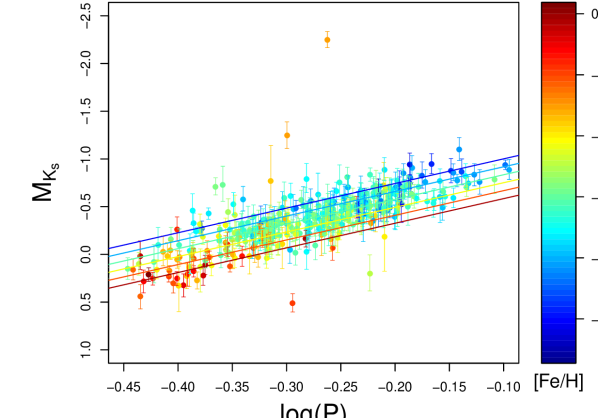
Figure 15: $PM_{K_{s}}$ distribution of 400 RRLs in our sample, for which absolute $M_{K_{s}}$ magnitudes were inferred from the model described in Section 4. The lines represent projections of the fit shown in the first portion of Table 4 onto the Magnitude-Period plane. The colour scale encodes metallicity values measured on the Zinn & West (1984) metallicity scale.

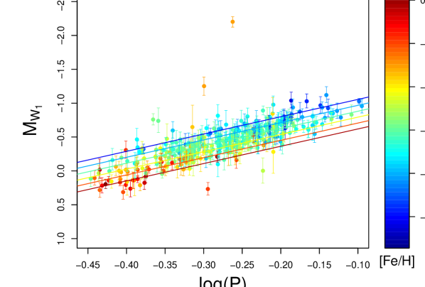
Figure 16: $PM_{W1}$ distribution of 397 RRLs from our sample, for which absolute $M_{W1}$ magnitudes were inferred from the model described in Section 4. The lines represent projections of the fit shown in the first portion of Table 4 onto the Magnitude-Period plane. The colour scale encodes metallicity values measured on the Zinn & West (1984) metallicity scale.

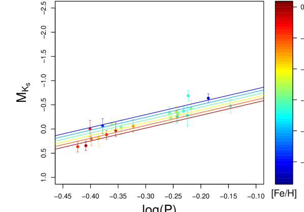
Figure 17: $PM_{K_{s}}$ distribution of 23 RRLs from our sample, for which absolute $M_{K_{s}}$ magnitudes were inferred from the model described in Section 4. The lines represent projections of the fit shown in the second portion of Table 4 onto the Magnitude-Period plane. The colour scale encodes metallicity values measured on the high-resolution spectroscopy metallicity scale.

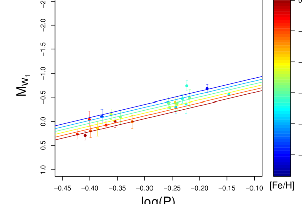
Figure 18: $PM_{W1}$ distribution of 23 RRLs from our sample, for which absolute $M_{W1}$ magnitudes were inferred from the model described in Section 4. The lines represent projections of the fit shown in the second portion of Table 4 onto the Magnitude-Period plane. The colour scale encodes metallicity values measured on the high-resolution spectroscopy metallicity scale.

We derived infrared $PM_{K_{\rm s}}Z$ and $PM_{W1}Z$ relations for the RRLs in our sample using the Bayesian approach described in Section 4 and inferring the parallax zero-point offset from the model. The near-infrared $PM_{K_{\rm s}}Z$ relation is based on a sample of 400 RRLs for which all needed information along with apparent $K_{\rm s}$ magnitudes and related uncertainties are available in Dambis et al. (2013) (see Section 2). To derive the $PM_{W1}Z$ relation we used a sample of 397 RRLs for which $W1$ magnitudes and related uncertainties are also available in Dambis et al. (2013). The coefficients of the resulting relations are summarised in the first section of Table 4 (row 3 and 4 respectively) and graphically shown in Figs. 15 and 16, where the colours encode the RRL metallicities on the Zinn & West (1984) metallicity scale. The slope in period we derive for the $PM_{K}Z$ relation is in perfect agreement with the literature values, while the metallicity slope is higher than found in previous empirical studies but in excellent agreement with the theoretical findings (e.g Bono et al. 2003, Catelan et al. 2004). The slope in period of the $PM_{W1}Z$ relation is slightly steeper than the literature values. We also find a non-negligible metallicity dependence, that is consistent with results from Neeley et al. (2017) and Sesar et al. (2017). The mean value of the parallax offset derived from fitting the linear $M_{V}-{\rm[Fe/H]}$ (Section 5.1) and the $PM_{K}Z$, $PM_{W1}Z$ relations of the full sample of RRLs is $-0.057$ mas, which is in very good agreement with the offset value found for RRLs by Arenou et al. (2018). In particular, the offset inferred from the model for the $PM_{W1}Z$ relation matches exactly the Arenou et al. (2018)’s value.

We have performed the fitting on our reduced sample of 23 RRLs both inferring the parallax offset as a parameter of the model and assuming a constant offset value of $-0.057$ mas. The resulting relations are presented in the second and third portions of Table 4. Figs. 17 and 18 graphically show the $PM_{K}Z$ and $PM_{W1}Z$ relations obtained from this reduced sample of 23 MW RRLs, when inferring the parallax offset as a parameter of the model. As with the RRL $M_{V}-{\rm[Fe/H]}$ relation the metallicity slope is significantly shallower for the reduced sample of 23 RRLs and in agreement within the uncertainties with values presented in the literature (e.g. Catelan et al. 2004, Neeley et al. 2017, Sesar et al. 2017). As in Section 5.2 we calculated the mean $M_{K_{\rm s}}$ and $M_{W1}$ absolute magnitudes of an RRL with metallicity [Fe/H]=$-1.5$ dex and period P=0.5238 days, which is the mean period of the RRLs in our sample. The resulting values are presented in column 6 of Table 4.

Fig. 19 shows the marginal posterior distributions in different one- and two-dimensional projection planes for the $W1$-band dataset. These distributions are representative/qualitatively similar to those obtained for the other models discussed in this study.

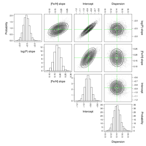
Figure 19: Marginal posterior distributions of the $W1$-band dataset in different one- and two-dimensional projections: from left to right, the $\log(P)$ and $\left[\mathrm{Fe/H}\right]$ coefficients, the intercept and the intrinsic dispersion. Each green line points towards the median of the corresponding one-dimensional posterior marginal distribution.

5.4 $M_{G}-{\rm[Fe/H]}$ relation

The Gaia DR2 catalogue contains magnitudes in the Gaia $G$-band ($330-1050$ nm) for $\sim 1.7$ billion sources and $G_{BP}$, $G_{RP}$ photometry derived from the integration of the blue and red photometer low-resolution spectra ($G_{BP}$: $330-680$ nm; $G_{RP}$: $630-1050$ nm) for $\sim 1.4$ billion sources (Evans et al., 2018). For sources confirmed to be RRLs Gaia DR2 also published intensity-averaged mean $G$, $G_{BP}$, $G_{RP}$ magnitudes computed by modelling the multi-band light curves over the whole pulsation cycle and extinction values in the $G$-band inferred from the RRL pulsation characteristics (Clementini et al., 2018). Specifically, intensity-averaged mean $G$ magnitudes are available for 306 of the RRLs in our sample and the $G$-band extinction values are available for 160 of them. We used the sample of 160 RRLs along with their metallicities from Dambis et al. (2013) and our Bayesian model with an adopted parallax offset of $-$0.057 mas to fit the RRL $M_{G}-{\rm[Fe/H]}$ relation. The relation is shown in the last portion of Table 4 and in Fig. 20. The corresponding RRL $G$-band absolute magnitude at [Fe/H]=$-1.5$ dex is $M_{G}=0.63\pm 0.08$ mag. This value is consistent with the $V$-band absolute magnitudes derived in Section 5.2 and can be used to infer an approximate estimation of distance to RRLs whose apparent mean magnitude and extinction in the $G$-band are available in the Gaia DR2 catalogue.

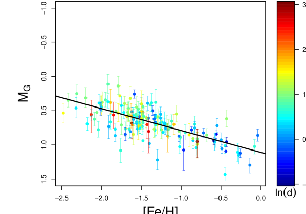
Figure 20: $M_{G}-{\rm[Fe/H]}$ relation defined by 160 RRLs in our sample, whose absolute $M_{G}$ magnitudes were inferred from the model described in Section 4. The solid line represents the linear fit. Its slope and zero-point are summarised in the last portion of Table 4. The colour scale encodes the (natural) logarithm of the inferred (true) distance measured in units of kpc.

6 Distance to the LMC

As traditionally done in this type of studies, in order to test the Gaia DR2 parallax-calibrated relations of RRLs derived in Section 5 we apply them to infer the distance to the LMC, a cornerstone of the cosmological distance ladder, whose distance has been measured in countless studies with different distance indicators and independent techniques. Following Gaia Collaboration et al. (2017), we considered 70 RRLs located close to the LMC bar, for which spectroscopically measured metallicities (Gratton et al., 2004), extinction, periods and photometry in the $V$ (Clementini et al., 2003) and $K_{\rm s}$ (Muraveva et al., 2015) bands, are available. No $W1$-band photometry is available for these 70 LMC RRLs, while intensity-averaged $G$ mean magnitudes are available for 44 of them. However, the $G$-band extinction values are available only for two of the stars in this sample. Hence, we only considered the $V$, $K_{\rm s}$ magnitudes and applied the linear and quadratic $M_{V}-{\rm[Fe/H]}$ relations and the $PM_{K}Z$ relations in Table 4, to infer the distance to each RRL individually and then computed the weighted mean of the distribution. The metallicity scale adopted by Gratton et al. (2004), is 0.06 dex more metal-rich than the Zinn & West (1984) metallicity scale. We subtracted 0.06 dex from the metallicities of the LMC RRLs to convert them to the Zinn & West (1984) metallicity scale when dealing with the relations based on the whole sample of RRLs. No correction was applied instead when using the relations based on the 23 MW RRLs with metal abundances obtained from high-resolution spectroscopy. The LMC distance moduli obtained with this procedure are summarised in the last column of Table 4 and plotted in Fig. 21, where they are shown to agree within 1 $\sigma$ uncertainty (grey dashed lines) with the very precise LMC modulus: $\mu=18.493\pm 0.008({\rm stat})\pm 0.047({\rm syst}$) mag inferred by Pietrzynski et al. (2013) from the analysis of eight eclipsing binaries in the LMC bar (grey solid line).

We do not plot in Fig. 21 distance moduli obtained from the relations defined by the sample of 23 RRLs and the parallax offset inferred from the model, because the offset is significantly overestimated ($-$0.142 mas) in this case and the corresponding moduli underestimated. On the other hand, the relations based on the sample of 23 MW RRLs and an assumed constant value of the parallax offset of $-0.057$ mas produce LMC distance moduli (green triangles) in very good agreement with the canonical value by Pietrzynski et al. (2013). To conclude, the LMC distance moduli obtained in this study using the Gaia DR2 parallaxes are in good agreement with the canonical value, once the Gaia DR2 parallax offset is properly accounted for.

Figure 21: Distance moduli of the LMC obtained from the $M_{V}-{\rm[Fe/H]}$ and $PM_{K}Z$ relations derived in this paper using the full sample of MW RRLs (blue filled circles; values in column 7 of the first portion of Table 4) and the sample of 23 MW RRLs with an assumed constant value of the parallax offset of $-0.057$ mas (green triangles; values in column 7 of the third portion of Table 4). See text for the details.

7 Summary and conclusions

Gaia Data Release 2 provides accurate parallaxes for an unprecedented, large number of MW RRLs. In this study we analysed a sample of 401 MW field RRLs, for which $V$, $K_{\mathrm{s}}$, and $W1$ photometry, metal abundances, extinction values and pulsation periods are available in the literature and accurate parallaxes have become available with the Gaia DR2. We compared the Gaia DR2 parallaxes with the parallax estimates for these RRLs available in the Hipparcos, HST and TGAS catalogues. We find a general good agreement of the Gaia DR2 parallaxes with the TGAS and the HST measurements, while agreement with the Hipparcos catalogue is less pronounced. The accuracy of the DR2 parallax measurements for RRLs showcases an impressive improvement achieved by Gaia both with respect to its predecessor Hipparcos and the TGAS measurements released in DR1, and rivals to other space-born estimates by cutting down about a factor of 5 the parallax uncertainty for RRLs measured with the HST.

With Gaia DR2 it is for the first time possible to determine the coefficients (slopes and zero-points) of the fundamental relations ($M_{V}-{\rm[Fe/H]}$, $PM_{K}Z$, $PM_{W1}Z$, as well as the Gaia $M_{G}-{\rm[Fe/H]}$ relation), that RRLs conform to on the basis of statistically significant samples of stars with accurate parallax measurements availble, that we do in this paper by applying a fully Bayesian approach that properly handles parallax measurements and biases affecting our sample of 401 MW RRLs. We find the dependence of the luminosity on metallicity to be higher than usually adopted in the literature. We show that this high metallicity dependence is not caused by our inference method, but likely arises from the actual distribution of the data and it is strictly connected with a possible offset affecting the Gaia DR2 parallaxes. This effect is much reduced for a sample of 23 MW RRLs with the metallicity estimated from high-resolution spectroscopy, which are closer to us and span a narrower range of the distances. However, we caution the reader that selection effects can potentially be stronger for nearby RRLs. Using our Bayesian approach we recover an offset of about $-0.057$ mas affecting the Gaia DR2 parallaxes of our full sample of about 400 RRLs, confirming previous findings by Arenou et al. (2018).

Our study demonstrates the effectiveness of the Gaia parallaxes to establish the cosmic distance ladder by recovering the canonical value of 18.49 mag for the distance modulus of the LMC, once the DR2 parallax offset is properly corrected for. We hence confirm that Gaia is on the right path and look forward to DR3, which is currently foreseen for end of 2020.

References

- Arenou et al. (2018) Arenou F. et al., 2018, arXiv:1804.09375
- Benedict et al. (2011) Benedict G. F. et al., 2011, AJ, 142, 187
- Bono et al. (2003) Bono, G., Caputo, F., Castellani, V., et al. 2003, MNRAS, 344, 1097
- Cacciari et al. (1992) Cacciari C., Clementini G., & Fernle, J. A., 1992, ApJ, 396, 219
- Cacciari & Clementini (2003) Cacciari C., & Clementini G., 2003, Stellar Candles for the Extragalactic Distance Scale, 635, 105
- Caputo, Marconi & Musella (2000a) Caputo F., Marconi M., & Musella I., 2000a, A&A, 354, 610
- Caputo et al. (2000b) Caputo F., Castellan, V., Marconi M., & Ripepi V. 2000b, MNRAS, 316, 819
- Cardelli et al. (1989) Cardelli J. A., Clayton G. C., & Mathis, J. S. 1989, ApJ, 345, 245
- Carpenter et al. (2017) Carpenter B. et al., 2017, Journal of Statistical Software, 76, 1
- Catelan et al. (2004) Catelan M., Pritzl B. J. & Smith H. A. E. 2004, sApJS, 154, 633
- Catelan & Cortés (2008) Catelan M., & Cortés C., 2008, ApJ, 676, L135
- Clementini et al. (1995) Clementini G., Carretta E., Gratton R., Merighi R., Mould, J. R., McCarthy J. K., 1995, AJ, 110, 2319
- Clementini et al. (2003) Clementini G., Gratton R., Bragaglia A., Carretta E., Di Fabrizio L., Maio M., 2003, AJ, 125, 1309
- Clementini et al. (2018) Clementini G. et al., 2018, arXiv:1805.02079
- Cutri et al. (2003) Cutri R. M., Skrutskie M. F., van Dyk S. et al., 2003, “The IRSA 2MASS All-Sky Point Source Catalog, NASA/IPAC Infrared Science Archive
- Dambis et al. (2013) Dambis A. K., Berdnikov L. N., Kniazev A. Y., Kravtsov V. V., Rastorguev A. S., Sefako R., Vozyakova O. V., 2013, MNRAS, 435, 3206
- Dambis et al. (2014) Dambis A. K., Rastorguev A. S., & Zabolotskikh M. V., 2014, MNRAS, 439, 3765
- de Grijs et al. (2014) de Grijs R., Wicker J. E. & Bono G., 2014, AJ, 147, 122
- Delgado et al. (2018) Delgado H. E., Sarro L. M., Clementini G., Muraveva T., & Garofalo A., 2018, arXiv:1803.01162
- Drimmel et al. (2003) Drimmel R., Cabrera-Lavers A., & López-Corredoira M., 2003, A&A, 409, 205
- Evans et al. (2018) Evans D. W. et al., 2018, arXiv:1804.09368
- Feast (1997) Feast M. W., 1997, MNRAS, 284, 761
- Feast et al. (2008) Feast M. W., Laney C. D., Kinman T. D., van Leeuwen F., & Whitelock P. A., 2008, MNRAS, 386, 2115
- Federici et al. (2012) Federici L., Cacciari C., Bellazzini M., Fusi Pecci F., Galleti S., Perina S., 2012, A&A, 544, A155
- Fernley (1994) Fernley J. A, 1994, A&A, 284, L16
- Fernley et al. (1998) Fernley J. A., Carney, B. W., Skillen, I., Cacciari, C., & Janes, K. 1998, MNRAS, 293, L61
- Fusi Pecci et al. (1996) Fusi Pecci F., Buonanno R., Cacciari C., Corsi C. E., Djorgovski S. G., Federici L., Ferraro F. R., Parmeggiani G., Rich R. M., 1996, AJ, 112, 1461