Algorithms and Theory
for Multiple-Source Adaptation

Abstract

This work includes a number of novel contributions for the multiple-source adaptation problem. We present new normalized solutions with strong theoretical guarantees for the cross-entropy loss and other similar losses. We also provide new guarantees that hold in the case where the conditional probabilities for the source domains are distinct. Moreover, we give new algorithms for determining the distribution-weighted combination solution for the cross-entropy loss and other losses. We report the results of a series of experiments with real-world datasets. We find that our algorithm outperforms competing approaches by producing a single robust model that performs well on any target mixture distribution. Altogether, our theory, algorithms, and empirical results provide a full solution for the multiple-source adaptation problem with very practical benefits.

1 Introduction

In many modern applications, often the learner has access to information about several source domains, including accurate predictors possibly trained and made available by others, but no direct information about a target domain for which one wishes to achieve a good performance. The target domain can typically be viewed as a combination of the source domains, that is a mixture of their joint distributions, or it may be close to such mixtures. In addition, often the learner does not have access to all source data simultaneously, for legitimate reasons such as privacy, storage limitation, etc. Thus the learner cannot simply pool all source data together to learn a predictor.

Such problems arise commonly in speech recognition where different groups of speakers (domains) yield different acoustic models and the problem is to derive an accurate acoustic model for a broader population that may be viewed as a mixture of the source groups (Liao, 2013). In object recognition, multiple image databases exist, each with its own bias and labeled categories (Torralba and Efros, 2011), but the target application may contain images which most closely resemble only a subset of the available training data. Finally, in sentiment analysis, accurate predictors may be available for sub-domains such as TVs, laptops and CD players, each previously trained on labeled data, but no labeled data or predictor may be at the learner’s disposal for the more general category of electronics, which can be modeled as a mixture of the sub-domains (Blitzer et al., 2007; Dredze et al., 2008).

The problem of transfer from a single source to a known target domain, either through unsupervised adaptation techniques (Gong et al., 2012; Long et al., 2015; Ganin and Lempitsky, 2015; Tzeng et al., 2015), or via lightly supervised ones (some amount of labeled data from the target domain) (Saenko et al., 2010; Yang et al., 2007; Hoffman et al., 2013; Girshick et al., 2014), has been extensively investigated in the past. Here, we focus on the problem of multiple-source domain adaptation and ask how the learner can combine relatively accurate predictors available for each source domain to derive an accurate predictor for any new mixture target domain? This is known as the multiple-source adaption (MSA) problem first formalized and analyzed theoretically by Mansour et al. (2008, 2009) and later studied for various applications such as object recognition (Hoffman et al., 2012; Gong et al., 2013a, b). Recently, Zhang et al. (2015) studied a causal formulation of this problem and analyzed the same combination rules of Mansour et al. (2008, 2009) for classification scenario. A closely related problem is also that of domain generalization (Pan and Yang, 2010; Muandet et al., 2013; Xu et al., 2014), where knowledge from an arbitrary number of related domains is combined to perform well on a previously unseen domain.

Mansour et al. (2008, 2009) gave strong theoretical guarantees for a distribution-weighted combination for the MSA problem, but they did not provide any algorithmic solution. Furthermore, the solution they proposed could not be used for loss functions such as cross-entropy, which require a normalized predictor. Their work also assumed a deterministic scenario (non-stochastic) with the same labeling function for all source domains.

This work makes a number of novel contributions to the MSA problem. We give new normalized solutions with strong theoretical guarantees for the cross-entropy loss and other similar losses. Our guarantees hold even when the conditional probabilities for the source domains are distinct. A by-product of our analysis is the extension of the theoretical results of Mansour et al. (2008, 2009) to the stochastic scenario, where there is a joint distribution over the input and output space.

Moreover, we give new algorithms for determining the distribution-weighted combination solution for the cross-entropy loss and other losses. We prove that the problem of determining that solution can be cast as a DC-programming (difference of convex) and prove explicit DC-decompositions for the cross-entropy loss and other losses. We also give a series of experimental results with several datasets demonstrating that our distribution-weighted combination solution is remarkably robust. Our algorithm outperforms competing approaches and performs well on any target mixture distribution.

Altogether, our theory, algorithms, and empirical results provide a full solution for the MSA problem with very practical benefits.

2 Problem setup

Let $\mathcal{X}$ denote the input space and $\mathcal{Y}$ the output space. We consider a multiple-source domain adaptation (MSA) problem in the general stochastic scenario where there is a distribution over the joint input-output space, $\mathcal{X}\times\mathcal{Y}$. This is a more general setup than the deterministic scenario in (Mansour et al., 2008, 2009), where a target function mapping from $\mathcal{X}$ to $\mathcal{Y}$ is assumed. This extension is needed for the analysis of the most common and realistic learning setups in practice. We will assume that $\mathcal{X}$ and $\mathcal{Y}$ are discrete, but the predictors we consider can take real values. Our theory can be straightforwardly extended to the continuous case with summations replaced by integrals in the proofs. We will identify a domain with a distribution over $\mathcal{X}\times\mathcal{Y}$ and consider the scenario where the learner has access to a predictor $h_{k}$, for each domain ${\mathscr{D}}_{k}$, $k=1,\ldots,p$.

We consider two types of predictor functions $h_{k}$, and their associated loss functions $L$ under the regression model (R) and the probability model (P) respectively,

$h_{k}\colon\mathcal{X}\to\mathbb{R}$	$L\colon\mathbb{R}\times\mathcal{Y}\to\mathbb{R}_{+}$	(R)
$h_{k}\colon\mathcal{X}\times\mathcal{Y}\to[0,1]$	$L\colon[0,1]\to\mathbb{R}_{+}$	(P)

We abuse the notation and write $L(h,x,y)$ to denote the loss of a predictor $h$ at point $(x,y)$, that is $L(h(x),y)$ in the regression model, and $L(h(x,y))$ in the probability model. We will denote by $\mathcal{L}({\mathscr{D}},h)$ the expected loss of a predictor $h$ with respect to the distribution ${\mathscr{D}}$:

$$\mathcal{L}({\mathscr{D}},h) =\mspace{-5.0mu}\operatorname*{\mathbb{E}}_{(x,y)\sim{\mathscr{D}}}\mspace{-5.0mu}\big{[}L(h,x,y)\big{]}=\mspace{-15.0mu}\sum_{(x,y)\in\mathcal{X}\times\mathcal{Y}}\mspace{-15.0mu}{\mathscr{D}}(x,y)L(h,x,y).$$

Much of our theory only assumes that $L$ is convex and continuous. But, we will be particularly interested in the case where in the regression model, $L(h(x),y)=(h(x)-y)^{2}$ is the squared loss, and where in the probability model, $L(h(x,y))=-\log h(x,y)$ is the cross-entropy loss ($\log$-loss).

We will assume that each $h_{k}$ is a relatively accurate predictor for the distribution ${\mathscr{D}}_{k}$: there exists $\epsilon>0$ such that $\mathcal{L}({\mathscr{D}}_{k},h_{k})\leq\epsilon$ for all $k\in[p]$. We will also assume that the loss of the source hypotheses $h_{k}$ is bounded, that is $L(h_{k},x,y)\leq M$ for all $(x,y)\in\mathcal{X}\times\mathcal{Y}$ and all $k\in[p]$.

In the MSA problem, the learner’s objective is to combine these predictors to design a predictor with small expected loss on a target domain that could be an arbitrary and unknown mixture of the source domains, the case we are particularly interested in, or even some other arbitrary distribution. It is worth emphasizing that the leaner has no knowledge of the target domain.

How do we combine the $h_{k}$s? Can we use a convex combination rule, $\sum_{k=1}^{p}\lambda_{k}h_{k}$, for some $\lambda\in\Delta$? In Appendix A (Lemmas 7 and 8) we show that no convex combination rule will perform well even in very simple MSA problems. These results generalize a previous lower bound of Mansour et al. (2008). Next, we show that the distribution-weighted combination rule is the right solution.

Extending the definition given by Mansour et al. (2008), we define the distribution-weighted combination of the functions $h_{k}$, $k\in[p]$ as follows. For any $z\in\Delta$, $\eta>0$, and $(x,y)\in\mathcal{X}\times\mathcal{Y}$,

$$h_{z}^{\eta}(x) =\sum_{k=1}^{p}\frac{z_{k}{\mathscr{D}}^{1}_{k}(x)+\eta\frac{{\mathscr{U}}^{1}(x)}{p}}{\sum_{k=1}^{p}z_{k}{\mathscr{D}}^{1}_{k}(x)+\eta{\mathscr{U}}^{1}(x)}h_{k}(x),$$ (R) (1)

$$h_{z}^{\eta}(x,y) =\sum_{k=1}^{p}\frac{z_{k}{\mathscr{D}}_{k}(x,y)+\eta\,\frac{{\mathscr{U}}(x,y)}{p}}{\sum_{j=1}^{p}z_{j}{\mathscr{D}}_{j}(x,y)+\eta\,{\mathscr{U}}(x,y)}h_{k}(x,y),$$ (P) (2)

where we denote by ${\mathscr{D}}^{1}(x)$ the marginal distribution over $\mathcal{X}$: ${\mathscr{D}}^{1}(x)=\sum_{y\in\mathcal{Y}}{\mathscr{D}}(x,y)$, and ${\mathscr{U}}^{1}(x)$ the uniform distribution over $\mathcal{X}$. This extension may seem technically straightforward in hindsight, but the form of the predictor was not immediately clear in the stochastic case.

3 Theoretical analysis

In this section, we present theoretical analyses of the general multiple-source adaptation setting. We first introduce our main result for the general stochastic scenario. Next, for the probability model with cross-entropy loss, we introduce a normalized distribution weighted combination and prove that it benefits from strong theoretical guarantees.

Our theoretical results rely on the measure of divergence between distributions. The one that naturally comes up in our analysis is the Rényi Divergence (Rényi, 1961). We will denote by ${\mathsf{d}}_{\alpha}({\mathscr{D}}\parallel{\mathscr{D}}^{\prime})=e^{{\mathsf{D}}_{\alpha}({\mathscr{D}}\parallel{\mathscr{D}}^{\prime})}$ the exponential of the $\alpha$-Rényi Divergence of two distributions ${\mathscr{D}}$ and ${\mathscr{D}}^{\prime}$. More details of the Rényi Divergence are given in Appendix F.

3.1 Stochastic scenario

Let ${\mathscr{D}}_{T}$ be an unknown target distribution. We will denote by ${\mathscr{D}}_{T}(\cdot|x)$ and ${\mathscr{D}}_{k}(\cdot|x)$ the conditional probability distribution on the target and the source domain respectively. Given the same input $x$, ${\mathscr{D}}_{T}(\cdot|x),{\mathscr{D}}_{k}(\cdot|x),k\in[p]$ are not necessarily the same. This is a novel extension that was not discussed in (Mansour et al., 2009), where in the deterministic scenario, exactly the same labeling function $f$ is assumed for all source domains.

For some choice of $\alpha>1$, define $\epsilon_{T}$ by

$$\epsilon_{T}=\max_{k\in[p]}\left[\underset{{\mathscr{D}}^{1}_{k}(x)}{\mathbb{E}}{\mathsf{d}}_{\alpha}\left({\mathscr{D}}_{T}(\cdot|x)\parallel{\mathscr{D}}_{k}(\cdot|x)\right)^{\alpha-1}\right]^{\frac{1}{\alpha}}\epsilon^{\frac{\alpha-1}{\alpha}}M^{\frac{1}{\alpha}}.$$

When the average divergence is small, $\alpha$ can be chosen to be very large and $\epsilon_{T}$ is close to $\epsilon$.

Let ${\mathscr{D}}_{T}$ be a mixture of source distributions, such that ${\mathscr{D}}^{1}_{T}\in\mathcal{D}^{1}=\{\sum_{k=1}^{p}\lambda_{k}{\mathscr{D}}^{1}_{k}:\lambda\in\Delta\}$ in the regression model (R), or ${\mathscr{D}}_{T}\in\mathcal{D}=\{\sum_{k=1}^{p}\lambda_{k}{\mathscr{D}}_{k}\colon\lambda\in\Delta\}$ in the probability model (P).

Theorem 1.

For any $\delta>0$, there exists $\eta>0$ and $z\in\Delta$ such that the following inequalities hold for any $\alpha>1$:

$$\mathcal{L}({\mathscr{D}}_{T},h_{z}^{\eta}) \leq\epsilon_{T}+\delta, (R)$$

$$\mathcal{L}({\mathscr{D}}_{T},h_{z}^{\eta}) \leq\epsilon+\delta. (P)$$

The proof is given in Appendix B. The learning guarantees for the regression and the probability model are slightly different, since the definitions of the distribution-weighted combinations are different for the two models. Theorem 1 shows the existence of $\eta>0$ and a mixture weight $z\in\Delta$ with a remarkable property: in the regression model (R), for any target distribution ${\mathscr{D}}_{T}$ whose conditional probability ${\mathscr{D}}_{T}(\cdot|x)$ is on average not too far away from ${\mathscr{D}}_{k}(\cdot|x)$ for any $k\in[p]$, and ${\mathscr{D}}^{1}_{T}\in\mathcal{D}^{1}$, the loss of $h_{z}^{\eta}$ on ${\mathscr{D}}_{T}$ is small. It is even more remarkable that, in the probability model (P), the loss of $h_{z}^{\eta}$ is at most $\epsilon$ on any target distribution ${\mathscr{D}}_{T}\in\mathcal{D}$. Therefore, $h_{z}^{\eta}$ is a robust hypothesis with favorable property for any such target distribution ${\mathscr{D}}_{T}$.

In many learning tasks, it is reasonable to assume that the conditional probability of the output labels is the same for all source domains. For example, a dog picture represents a dog regardless of whether the dog appears in an individual’s personal set of pictures or in a broader database of pictures from multiple individuals. This is a straightforward extension of the assumption adopted by Mansour et al. (2008) in the deterministic scenario, where exactly the same labeling function $f$ is assumed for all source domains. Then ${\mathscr{D}}_{T}(\cdot|x)={\mathscr{D}}_{k}(\cdot|x),\forall k\in[p]$. By definition, ${\mathsf{d}}_{\alpha}\left({\mathscr{D}}_{T}(\cdot|x)\parallel{\mathscr{D}}_{k}(\cdot|x)\right)=1$. Let $\alpha\to+\infty$, we recover the main result of Mansour et al. (2008).

Corollary 2.

Assume the conditional probability ${\mathscr{D}}_{k}(\cdot|x)$ does not depend on $k$. Let ${\mathscr{D}}_{\lambda}$ be an arbitrary mixture of source domains, $\lambda\in\Delta$. For any $\delta>0$, there exists $\eta>0$ and $z\in\Delta$, such that $\mathcal{L}({\mathscr{D}}_{\lambda},h_{z}^{\eta})\leq\epsilon+\delta$.

Corollary 2 shows the existence of a mixture weight $z\in\Delta$ and $\eta>0$ with a remarkable property: for any $\delta>0$, regardless of which mixture weight $\lambda\in\Delta$ defines the target distribution, the loss of $h_{z}^{\eta}$ is at most $\epsilon+\delta$, that is arbitrarily close to $\epsilon$. $h_{z}^{\eta}$ is therefore a robust hypothesis with a favorable property for any mixture target distribution.

To cover the realistic cases in applications, we further extend this result to the case where the distributions ${\mathscr{D}}_{k}$ are not directly available to the learner, and instead estimates $\widehat{\mathscr{D}}_{k}$ have been derived from data, and further to the case where the target distribution ${\mathscr{D}}_{T}$ is not a mixture of source distributions (Corollary 11 in Appendix B). We will denote by $\widehat{h}_{z}^{\eta}$ the distribution-weighted combination rule based on the estimates $\widehat{\mathscr{D}}_{k}$. Our learning guarantee for $\widehat{h}_{z}^{\eta}$ depends on the Rényi divergence of $\widehat{\mathscr{D}}_{k}$ and ${\mathscr{D}}_{k}$, as well as the Rényi divergence of ${\mathscr{D}}_{T}$ and the family of source mixtures.

3.2 Probability model with the cross-entropy loss

Next, we discuss the special case where $L$ coincide with the cross-entropy loss in the probability model, and present an analysis for a normalized distribution-weighted combination solution. This analysis is a complement to Theorem 1, which only works for the unnormalized hypothesis $h_{z}^{\eta}(x,y)$.

The cross-entropy loss assumes normalized hypotheses. Thus, the source functions are normalized for every $x$: $\sum_{y\in\mathcal{Y}}h_{k}(x,y)=1,\ \forall x\in\mathcal{X},\forall k\in[p]$. For any $z\in\Delta$, $\eta>0$, we define the normalized weighted combination $\overline{h}_{z}^{\eta}(x,y)$ that is based on $h_{z}^{\eta}(x,y)$ in (2):

$$\overline{h}_{z}^{\eta}(x,y)=\frac{h_{z}^{\eta}(x,y)}{\overline{h}_{z}^{\eta}(x)},\quad\text{where }\overline{h}_{z}^{\eta}(x)=\sum_{y\in\mathcal{Y}}h_{z}^{\eta}(x,y).$$

We will first assume the conditional probability ${\mathscr{D}}_{k}(\cdot|x)$ does not depend on $k$.

Theorem 3.

Assume there exists $\mu>0$ such that ${\mathscr{D}}_{k}(x,y)\geq\mu{\mathscr{U}}(x,y)$ for all $k\in[p]$ and $(x,y)\in\mathcal{X}\times\mathcal{Y}$. Then, for any $\delta>0$, there exists $\eta>0$ and $z\in\Delta$, such that $\mathcal{L}({\mathscr{D}}_{\lambda},\overline{h}_{z}^{\eta})\leq\epsilon+\delta$  for any mixture parameter $\lambda\in\Delta$.

The result of Theorem 3 admits the same favorable property as that of Corollary 2. It can also be extended to the case of arbitrary target distributions and estimated densities. When the conditional probabilities are different across the source domains, we propose a marginal distribution-weighted combination rule, which is already normalized. We can directly apply Theorem 1 to it and achieve favorable guarantees. More details are given in Appendix C.

These results are non-trivial and important, as they provide a guarantee for an accurate and robust predictor for a commonly used loss function, the cross-entropy loss.

4 Algorithms

We have shown that, for both the regression and the probability model, there exists a vector $z$ defining a distribution-weighted combination hypothesis $h_{z}^{\eta}$ that admits very favorable guarantees. But how we find a such $z$? This is a key question in the MSA problem which was not addressed by Mansour et al. (2008, 2009): no algorithm was previously reported to determine the mixture parameter $z$ (even for the deterministic scenario). Here, we give an algorithm for determining that vector $z$.

In this section, we give practical and efficient algorithms for finding the vector $z$ in the important cases of the squared loss in the regression model, or the cross-entropy loss in the probability model, by leveraging the differentiability of the loss functions. We first show that $z$ is the solution of a general optimization problem. Next, we give a DC-decomposition (difference of convex decomposition) of the objective for both models, thereby proving an explicit DC-programming formulation of the problem. This leads to an efficient DC algorithm that is guaranteed to converge to a stationary point. Additionally, we show that it is straightforward to test if the solution obtained is the global optimum. While we are not proving that the local stationary point found by our algorithm is the global optimum, empirically, we observe that that is indeed the case.

4.1 Optimization problem

Theorem 1 shows that the hypothesis $h_{z}^{\eta}$ based on the mixture parameter $z$ benefits from a strong generalization guarantee. A key step in proving Theorem 1 is to show the following lemma.

Lemma 4.

For any $\eta,\eta^{\prime}>0$, there exists $z\in\Delta$, with $z_{k}\neq 0$ for all $k\in[p]$, such that the following holds for the distribution-weighted combining rule $h_{z}^{\eta}$:

$$\forall k\in[p],\quad\mathcal{L}({\mathscr{D}}_{k},h_{z}^{\eta})\leq\sum_{j=1}^{p}z_{j}\mathcal{L}({\mathscr{D}}_{j},h_{z}^{\eta})+\eta^{\prime}.$$ (3)

Lemma 4 indicates that for the solution $z$, $h_{z}^{\eta}$ has essentially the same loss on all source domains. Thus, our problem consists of finding a parameter $z$ verifying this property. This, in turn, can be formulated as a min-max problem: $\min_{z\in\Delta}\max_{k\in[p]}\mathcal{L}({\mathscr{D}}_{k},h_{z}^{\eta})-\mathcal{L}({\mathscr{D}}_{z},h_{z}^{\eta}),$ which can be equivalently formulated as the following optimization problem:

$$\min_{z\in\Delta,\gamma\in\mathbb{R}}\ \gamma\quad\text{s.t.}\ \mathcal{L}({\mathscr{D}}_{k},h_{z}^{\eta})-\mathcal{L}({\mathscr{D}}_{z},h_{z}^{\eta})\leq\gamma,\,\forall k\in[p].$$ (4)

4.2 DC-decomposition

We provide explicit DC decompositions of the objective of Problem (4) for the regression model with the squared loss and the probability model with the cross-entropy loss. The full derivations are given in Appendix D.

We first rewrite $h^{\eta}_{z}$ as the division of two affine functions for the regression model (R) and the probability model (P): $h_{z}=J_{z}/K_{z}$, where

$\displaystyle J_{z}(x)=\sum_{k=1}^{p}z_{k}{\mathscr{D}}^{1}_{k}(x)h_{k}(x)+\frac{\eta}{p}{\mathscr{U}}^{1}(x)h_{k}(x)$,	$\displaystyle K_{z}(x)={\mathscr{D}}^{1}_{z}(x)+\eta\,{\mathscr{U}}^{1}(x)$,	(R)
$\displaystyle J_{z}(x,y)=\sum_{k=1}^{p}z_{k}{\mathscr{D}}_{k}(x,y)h_{k}(x,y)+\frac{\eta}{p}{\mathscr{U}}(x,y)h_{k}(x,y)$,	$\displaystyle K_{z}(x,y)=D_{z}(x,y)+\eta\,{\mathscr{U}}(x,y)$	(P)

Proposition 5 (Regression model, square loss).

Let $L$ be the squared loss. Then, for any $k\in[p]$, $\mathcal{L}({\mathscr{D}}_{k},h_{z}^{\eta})-\mathcal{L}({\mathscr{D}}_{z},h_{z}^{\eta})=u_{k}(z)-v_{k}(z)$, where $u_{k}$ and $v_{k}$ are convex functions defined for all $z$ by

$$u_{k}(z) =\mathcal{L}\left({\mathscr{D}}_{k}+\eta{\mathscr{U}}^{1}{\mathscr{D}}_{k}(\cdot|x),h_{z}^{\eta}\right)-2M\sum_{x}({\mathscr{D}}^{1}_{k}+\eta{\mathscr{U}}^{1})(x)\log K_{z}(x),$$

$$v_{k}(z) =\mathcal{L}\left({\mathscr{D}}_{z}+\eta{\mathscr{U}}^{1}{\mathscr{D}}_{k}(\cdot|x),h_{z}^{\eta}\right)-2M\sum_{x}({\mathscr{D}}^{1}_{k}+\eta{\mathscr{U}}^{1})(x)\log K_{z}(x).$$

Proposition 6 (Probability model, cross-entropy loss).

Let $L$ be the cross-entropy loss. Then, for $k\in[p]$, $\mathcal{L}({\mathscr{D}}_{k},h_{z}^{\eta})-\mathcal{L}({\mathscr{D}}_{z},h_{z}^{\eta})=u_{k}(z)-v_{k}(z)$, where $u_{k}$ and $v_{k}$ are convex functions:

$$u_{k}(z) =-\sum_{x,y}\big{[}{\mathscr{D}}_{k}(x,y)+\eta\,{\mathscr{U}}(x,y)\big{]}\log J_{z}(x,y),$$

$$v_{k}(z) =\sum_{x,y}K_{z}(x,y)\log\left[\frac{K_{z}(x,y)}{J_{z}(x,y)}\right]-\left[{\mathscr{D}}_{k}(x,y)+\eta\,{\mathscr{U}}(x,y)\right]\log K_{z}(x,y).$$

4.3 DC algorithm

Our DC decompositions prove that the optimization problem (4) can be cast as the following variational form of a DC-programming problem (Tao and An, 1997, 1998; Sriperumbudur and Lanckriet, 2012):

$$\min_{z\in\Delta,\gamma\in\mathbb{R}}\gamma\quad\text{s.t.}\big{(}u_{k}(z)-v_{k}(z)\leq\gamma\big{)}\wedge\big{(}-z_{k}\leq 0\big{)}\wedge\big{(}\textstyle\sum_{k=1}^{p}z_{k}-1=0\big{)},\quad\forall k\in[p].$$ (5)

The DC-programming algorithm works as follows. Let $(z_{t})_{t}$ be the sequence defined by repeatedly solving the following convex optimization problem:

$$z_{t+1} \in\operatorname*{\rm argmin}_{z,\gamma\in\mathbb{R}}\ \gamma$$ (6)

s.t. $$\ \big{(}u_{k}(z)-v_{k}(z_{t})-(z-z_{t})\nabla v_{k}(z_{t})\leq\gamma\big{)}\wedge\big{(}-z_{k}\leq 0\big{)}\wedge\big{(}\textstyle\sum_{k=1}^{p}z_{k}-1=0\big{)},\quad\forall k\in[p],$$

where $z_{0}\in\Delta$ is an arbitrary starting value. Then, $(z_{t})_{t}$ is guaranteed to converge to a local minimum of Problem (4) (Yuille and Rangarajan, 2003; Sriperumbudur and Lanckriet, 2012). Note that Problem (6) is a relatively simple optimization problem: $u_{k}(z)$ is a weighted sum of the negative logarithm of an affine function of $z$, plus a weighted sum of rational functions of $z$ (squared loss), and all other terms appearing in the constraints are affine functions of $z$.

Problem (4) seeks a parameter $z$ verifying $\mathcal{L}({\mathscr{D}}_{k},h_{z}^{\eta})-\mathcal{L}({\mathscr{D}}_{z},h_{z}^{\eta})\leq\gamma$, for all $k\in[p]$ for an arbitrarily small value of $\gamma$. Since $\mathcal{L}({\mathscr{D}}_{z},h_{z}^{\eta})=\sum_{k=1}^{p}z_{k}\mathcal{L}({\mathscr{D}}_{k},h_{z}^{\eta})$ is a weighted average of the expected losses $\mathcal{L}({\mathscr{D}}_{k},h_{z}^{\eta})$, $k\in[p]$, the solution $\gamma$ cannot be negative. Furthermore, by Lemma 4, a parameter $z$ verifying that inequality exists for any $\gamma>0$. Thus, the global solution $\gamma$ of Problem (4) must be close to zero. This provides us with a simple criterion for testing the global optimality of the solution $z$ we obtain using a DC-programming algorithm with a starting parameter $z_{0}$.

5 Experiments

This section reports the results of our experiments with our DC-programming algorithm for finding a robust domain generalization solution when using squared loss and cross-entropy loss. We first evaluate our algorithm using an artificial dataset assuming known densities where we may compare our result to the global solution and found that indeed our global objective approached the known optimum of zero (see Appendix E for more details). Next, we evaluate our DC-programming solution applied to real-world datasets: a sentiment analysis dataset (Blitzer et al., 2007) for squared loss, a visual domain adaptation benchmark dataset Office (Saenko et al., 2010), as well as a generalization of digit recognition task, for cross-entropy loss.

For all real-world datasets, the probability distributions ${\mathscr{D}}_{k}$ are not readily available to the learner. However, Corollary 11 extends the learning guarantees of our solution to the case where an estimate $\widehat{\mathscr{D}}_{k}$ is used in lieu of the ideal distribution ${\mathscr{D}}_{k}$. Thus, we used standard density estimation methods to derive an estimate $\widehat{\mathscr{D}}_{k}$ for each $k\in[p]$. While density estimation can be a difficult task in general, for our purpose straightforward techniques are sufficient for our predictor $\widehat{h}_{z}^{\eta}$ to achieve a high performance, since the approximate densities only serve to indicate the relative importance of each source domain. We give full details of our density estimation procedure in Appendix E.

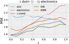
(a)

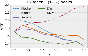
(b)

Figure 1: MSE sentiment analysis under mixture of two domains: (left) dvd and electronics or (right) kitchen and books.

5.1 Sentiment analysis task for squared loss

We use the sentiment analysis dataset proposed by Blitzer et al. (2007) and used for multiple-source adaptation by Mansour et al. (2008, 2009). This dataset consists of product review text and rating labels taken from four domains: books (B), dvd (D), electronics (E), and kitchen (K), with $2000$ samples for each domain. We defined a vocabulary of $2\mathord{,}500$ words that occur at least twice at the intersection of the four domains. These words were used to define feature vectors, where every sample is encoded by the number of occurrences of each word. We trained our base hypotheses using support vector regression (SVR) with same hyper-parameters as in (Mansour et al., 2008, 2009).

Table 1: MSE on the sentiment analysis dataset of source-only baselines for each domain, K,D, B,E, the uniform weighted predictor unif, KMM, and the distribution-weighted method DW based on the learned $z$. DW outperforms all competing baselines.

	Test Data
	K	D	B	E	KD	BE	DBE	KBE	KDB	KDB	KDBE
K	1.46$\pm$0.08	2.20$\pm$0.14	2.29$\pm$0.13	1.69$\pm$0.12	1.83$\pm$0.08	1.99$\pm$0.10	2.06$\pm$0.07	1.81$\pm$0.07	1.78$\pm$0.07	1.98$\pm$0.06	1.91$\pm$0.06
D	2.12$\pm$0.08	1.78$\pm$0.08	2.12$\pm$0.08	2.10$\pm$0.07	1.95$\pm$0.07	2.11$\pm$0.07	2.00$\pm$0.06	2.11$\pm$0.06	2.00$\pm$0.06	2.01$\pm$0.06	2.03$\pm$0.06
B	2.18$\pm$0.11	2.01$\pm$0.09	1.73$\pm$0.12	2.24$\pm$0.07	2.10$\pm$0.09	1.99$\pm$0.08	1.99$\pm$0.05	2.05$\pm$0.06	2.14$\pm$0.06	1.98$\pm$0.06	2.04$\pm$0.05
E	1.69$\pm$0.09	2.31$\pm$0.12	2.40$\pm$0.11	1.50$\pm$0.06	2.00$\pm$0.09	1.95$\pm$0.07	2.07$\pm$0.06	1.86$\pm$0.04	1.84$\pm$0.06	2.14$\pm$0.06	1.98$\pm$0.05
unif	1.62$\pm$0.05	1.84$\pm$0.09	1.86$\pm$0.09	1.62$\pm$0.07	1.73$\pm$0.06	1.74$\pm$0.07	1.77$\pm$0.05	1.70$\pm$0.05	1.69$\pm$0.04	1.77$\pm$0.04	1.74$\pm$0.04
KMM	1.63$\pm$0.15	2.07$\pm$0.12	1.93$\pm$0.17	1.69$\pm$0.12	1.83$\pm$0.07	1.82$\pm$0.07	1.89$\pm$0.07	1.75$\pm$0.07	1.78$\pm$0.06	1.86$\pm$0.09	1.82$\pm$0.06
DW(ours)	1.45$\pm$0.08	1.78$\pm$0.08	1.72$\pm$0.12	1.49$\pm$0.06	1.62$\pm$0.07	1.61$\pm$0.08	1.66$\pm$0.05	1.56$\pm$0.04	1.58$\pm$0.05	1.65$\pm$0.04	1.61$\pm$0.04

We compare our method (DW) against each source hypothesis, $h_{k}$. We also compute a privileged baseline using the oracle $\lambda$ mixing parameter, $\lambda$-comb: $\sum_{k=1}^{p}\lambda_{k}h_{k}$. $\lambda$-comb is of course not accessible in practice since the target mixture $\lambda$ is not known to the user. We also compare against a previously proposed domain adaptation algorithm (Huang et al., 2006) known as KMM. It is important to note that the KMM model requires access to the unlabeled target data during adaptation and learns a new predictor for every target domain, while DW does not use any target data. Thus KMM operates in a favorable learning setting when compared to our solution.

We first considered the same test scenario as in (Mansour et al., 2008), where the target is a mixture of two source domains. The plots of Figures 1a and 1b report the results of our experiments. They show that our distribution-weighted predictor DW outperforms all baseline predictors despite the privileged learning scenarios of $\lambda$-comb and KMM. We didn’t compare to the “weighted” predictor in empirical studies by Mansour et al. (2008) because it is not a real solution, but rather taking the unknown target mixture $\lambda$ as $z$ to compute $h_{z}$.

Next, we compared the performance of DW with accessible baseline predictors on various target mixtures. Since $\lambda$ is not accessible in practice, We replace $\lambda$-comb with the uniform combination of all hypotheses (unif), $\sum_{k=1}^{p}h_{k}/p$. Table 1 reports the mean and standard deviations of MSE over $10$ repetitions. Each column corresponds to a different target test data source. Our distribution-weighted method DW outperforms all baseline predictors across all test domains. Observe that, even when the target is a single source domain, our method successfully outperforms the predictor which is trained and tested on the same domain. Results on more target mixtures are available in Appendix E.

Table 2: Digit dataset statistics.

	SVHN	MNIST	USPS
# train images	73,257	60,000	7,291
# test images	26,032	10,000	2,007
image size	32x32	28x28	16x16
color	rgb	gray	gray

Table 3: Digit dataset accuracy: We report accuracy across six possible test domains.

	Test Data
	svhn	mnist	usps	mu	su	sm	smu	mean
CNN-s	92.3	66.9	65.6	66.7	90.4	85.2	84.2	78.8
CNN-m	15.7	99.2	79.7	96.0	20.3	38.9	41.0	55.8
CNN-u	16.7	62.3	96.6	68.1	22.5	29.4	32.9	46.9
CNN-unif	75.7	91.3	92.2	91.4	76.9	80.0	80.7	84.0
DW (ours)	91.4	98.8	95.6	98.3	91.7	93.5	93.6	94.7
CNN-joint	90.9	99.1	96.0	98.6	91.3	93.2	93.3	94.6

Table 4: Office dataset accuracy: We report accuracy across six possible test domains. We show performance all baselines: CNN-a,w,d, CNN-unif, DW based on the learned $z$, and the jointly trained model CNN-joint. DW outperforms all competing models.

	Test Data
	amazon	webcam	dslr	aw	ad	wd	awd	mean
CNN-a	75.7 $\pm$ 0.3	53.8 $\pm$ 0.7	53.4 $\pm$ 1.3	71.4 $\pm$ 0.3	73.5 $\pm$ 0.2	53.6 $\pm$ 0.8	69.9 $\pm$ 0.3	64.5 $\pm$ 0.6
CNN-w	45.3 $\pm$ 0.5	91.1 $\pm$ 0.8	91.7 $\pm$ 1.2	54.4 $\pm$ 0.5	50.0 $\pm$ 0.5	91.3 $\pm$ 0.8	57.5 $\pm$ 0.4	68.8 $\pm$ 0.7
CNN-d	50.4 $\pm$ 0.4	89.6 $\pm$ 0.9	90.9 $\pm$ 0.8	58.3 $\pm$ 0.4	54.6 $\pm$ 0.4	90.0 $\pm$ 0.7	61.0 $\pm$ 0.4	70.7 $\pm$ 0.6
CNN-unif	69.7 $\pm$ 0.3	93.1 $\pm$ 0.6	93.2 $\pm$ 0.9	74.4 $\pm$ 0.4	72.1 $\pm$ 0.3	93.1 $\pm$ 0.5	75.9 $\pm$ 0.3	81.6 $\pm$ 0.5
DW (ours)	75.2 $\pm$ 0.4	93.7 $\pm$ 0.6	94.0 $\pm$ 1.0	78.9 $\pm$ 0.4	77.2 $\pm$ 0.4	93.8 $\pm$ 0.6	80.2 $\pm$ 0.3	84.7 $\pm$ 0.5
CNN-joint	72.1 $\pm$ 0.3	93.7 $\pm$ 0.5	93.7 $\pm$ 0.5	76.4 $\pm$ 0.4	76.4 $\pm$ 0.4	93.7 $\pm$ 0.5	79.3 $\pm$ 0.4	83.6 $\pm$ 0.4

5.2 Recognition tasks for cross-entropy loss

We consider two real-world domain adaptation tasks: a generalization of digit recognition task, and a standard visual adaptation Office dataset.

For each individual domain, we train a convolutional neural network (CNN) and use the output from the softmax score layer as our base predictors $h_{k}$. We compute the uniformly weighted combination of source predictors, $h_{\texttt{unif}}=\sum_{k=1}^{p}h_{k}/p$. As a privileged baseline, we also train a model on all source data combined, $h_{\texttt{joint}}$. Note, this approach is often not feasible if independent entities contribute classifiers and densities, but not full training datasets. Thus this approach is not consistent with our scenario, and it operates in a much more favorable learning setting than our solution. Finally, our distribution weighted predictor DW is computed with $h_{k}$s, density estimates, and our learned weighting, $z$. Our baselines then consists of the classifiers from $h_{k}$, $h_{\texttt{unif}}$, $h_{\texttt{joint}}$, and DW.

We begin our study with a generalization of digit recognition task, which consists of three digit recognition datasets: Google Street View House Numbers (SVHN), MNIST, and USPS. Dataset statistics as well as example images can be found in Table 3. We train the ConvNet (or CNN) architecture following  Taigman et al. (2017) as our source models and joint model. We use the second fully-connected layer’s output as our features for density estimation, and the output from the softmax score layer as our predictors. We use the full training sets per domain to learn the source model and densities. Note, these steps are completely isolated from one another and may be performed by unique entities and in parallel. Finally, for our DC-programming algorithm we use small subset of 200 real image-label pairs from each domain to learn the parameter $z$.

Our next experiment uses the standard visual adaptation Office dataset, which has 3 domains: amazon, webcam, and dslr. The dataset contains 31 recognition categories of objects commonly found in an office environment. There are 4110 images total with 2817 from amazon, 795 from webcam, and 498 from dslr. We follow the standard protocol from Saenko et al. (2010), whereby 20 labeled examples are available for training from the amazon domain and 8 labeled examples are available from both the webcam and dslr domains. The remaining examples from each domain are used for testing. We use the AlexNet Krizhevsky et al. (2012) ConvNet (CNN) architecture, and use the output from softmax score layer as our base predictors, pre-trained on ImageNet and use fc7 activations as our features for density estimation Donahue et al. (2014).

We report the performance of our method and that of baselines on the digit recognition dataset in Table 3, and report the performance on the Office dataset in Table 4. On both datasets, we evaluate on various test distributions: each individual domain, the combination of each two domains and the fully combined set. When the test distribution equals one of the source distributions, our distribution-weighted classifier successfully outperforms (webcam,dslr) or maintains performance of the classifier which is trained and tested on the same domain. For the more realistic scenario where the target domain is a mixture of any two or all three source domains, the performance of our method is comparable or marginally superior to that of the jointly trained network, despite the fact that we do not retrain any network parameters in our method and that we only use a small number of per-domain examples to learn the distribution weights – an optimization which may be solved on a single CPU in a matter of seconds for this problem. This again demonstrates the robustness of our distribution-weighted combined classifier to a varying target domain.

6 Conclusion

We presented practically applicable multiple-source domain adaptation algorithms for the cross-entropy loss and other similar losses. These algorithms benefit from very favorable theoretical guarantees that we extended to the stochastic setting. Our empirical results further demonstrate empirically their effectiveness and their importance in adaptation problems.

Appendix A Lower bounds for convex combination rules

In this section, we give lower bounds for convex combination rule, for both squared loss and cross-entropy loss. For any $\alpha\in\Delta$, define the convex combination rule for the regression and the probability model as follows:

$$g_{\alpha}(x) =\sum_{k=1}^{p}\alpha_{k}h_{k}(x),$$ (R) (7)

$$g_{\alpha}(x,y) =\sum_{k=1}^{p}\alpha_{k}h_{k}(x,y).$$ (P) (8)

Lemma 7 (Regression model, squared loss).

There is a mixture adaptation problem for which the expected squared loss of $g_{\alpha}$ is $\frac{1}{4}$.

Proof.

Let $\mathcal{X}=\{a,b\}$, and $\mathcal{Y}=\{0,1\}$. Consider ${\mathscr{D}}_{0}(x,y)=1_{x=a,y=0}$, and $h_{0}(x)=0$; ${\mathscr{D}}_{1}(x,y)=1_{x=b,y=1}$, and $h_{1}(x)=1$. Consider the target distribution ${\mathscr{D}}_{T}=\frac{1}{2}{\mathscr{D}}_{0}+\frac{1}{2}{\mathscr{D}}_{1}$. Then, for any convex combination rule $g_{\alpha}=\alpha h_{0}+(1-\alpha)h_{1}=1-\alpha$,

$$\left(\frac{1}{2}\right)^{2} =\left(\frac{1}{2}\alpha+\frac{1}{2}(1-\alpha)\right)^{2}=\Bigg{(}\sum_{(x,y)\in\mathcal{X}\times\mathcal{Y}}{\mathscr{D}}_{T}(x,y)|g_{\alpha}(x)-y|\Bigg{)}^{2}$$

$$\leq\sum_{(x,y)\in\mathcal{X}\times\mathcal{Y}}{\mathscr{D}}_{T}(x,y)(g_{\alpha}(x)-y)^{2}=\mathcal{L}({\mathscr{D}}_{T},g_{\alpha}).$$

∎

Note that the hypotheses $h_{0}$ and $h_{1}$ have zero error on their own domain, i.e. $\epsilon=0$. However, no convex combination rule will perform well on the target distribution ${\mathscr{D}}_{T}$.

Lemma 8 (Probability Model, cross-entropy loss).

There is a mixture adaptation problem for which the expected cross-entropy loss of $g_{\alpha}$ is $\log(p)$.

Proof.

Let $\mathcal{X}=\{x_{1},\dots,x_{k}\}$, and $\mathcal{Y}=\{y_{1},\dots,y_{k}\}$. Consider ${\mathscr{D}}_{k}(x,y)=1_{x=x_{k},y=y_{k}}$, and $h_{k}(x,y)=1_{y=y_{k}}$. Consider the largest cross-entropy loss of $g_{\alpha}$ on any target mixture ${\mathscr{D}}_{\lambda}(x,y)$:

$$\max_{\lambda\in\Delta}\mathcal{L}({\mathscr{D}}_{\lambda},g_{\alpha}) =\max_{\lambda\in\Delta}\sum_{k=1}^{p}-\lambda_{k}\log(\alpha_{k})=\max_{k\in[p]}\left[-\log(\alpha_{k})\right].$$

Choosing $\alpha\in\Delta$ to minimize that adversarial loss gives

$$\min_{\alpha\in\Delta}\max_{k\in[p]}\left[-\log(\alpha_{k})\right]=\log(p).$$

Therefore any convex combination rule $g_{\alpha}$ incurs at least a loss of $\log(p)$. ∎

Again, the base hypotheses $h_{k}$s have zero error on their own domain, yet there is no convex combination rule that is robust against any target mixture.

Appendix B Theoretical analysis for the stochastic scenario

In this section, we give a series of theoretical results for the general stochastic scenario with their full proofs. We will separate the proofs for the regression model (Appendix B.1) and the probability model (Appendix B.2), since the definitions of the distribution weighted combination are different in the two models.

B.1 Regression model

The proofs for the regression model (R) are presented in the following order: we first assume the conditional probabilities are the same across source domains, and prove Lemma 4; using that, we prove Corollary 2 and Corollary 11. Finally, we relax the assumption of same conditionals, and prove Theorem 12, which a stronger version of Theorem 1.

Our proofs make use of the following Fixed-Point Theorem of Brouwer.

Theorem 9.

For any compact and convex non-empty set $C\subset\mathbb{R}^{p}$ and any continuous function $f\colon C\rightarrow C$, there is a point $x\in C$ such that $f(x)=x$.

Lemma 4.

For any $\eta,\eta^{\prime}>0$, there exists $z\in\Delta$, with $z_{k}\neq 0$ for all $k\in[p]$, such that the following holds for the distribution-weighted combining rule $h_{z}^{\eta}$:

$$\forall k\in[p],\quad\mathcal{L}({\mathscr{D}}_{k},h_{z}^{\eta})\leq\sum_{j=1}^{p}z_{j}\mathcal{L}({\mathscr{D}}_{j},h_{z}^{\eta})+\eta^{\prime}.$$ (9)

Proof.

Consider the mapping $\Phi\colon\Delta\to\Delta$ defined for all $z\in\Delta$ by

$$[\Phi(z)]_{k}=\frac{z_{k}\,\mathcal{L}({\mathscr{D}}_{k},h_{z}^{\eta})+\frac{\eta^{\prime}}{p}}{\sum_{j=1}^{p}z_{j}\mathcal{L}({\mathscr{D}}_{j},h_{z}^{\eta})+\eta^{\prime}}.$$

$\Phi$ is continuous since $\mathcal{L}({\mathscr{D}}_{k},h_{z}^{\eta})$ is a continuous function of $z$ and since the denominator is positive ($\eta^{\prime}>0$). Thus, by Brouwer’s Fixed Point Theorem, there exists $z\in\Delta$ such that $\Phi(z)=z$. For that $z$, we can write

$$z_{k}=\frac{z_{k}\,\mathcal{L}({\mathscr{D}}_{k},h_{z}^{\eta})+\frac{\eta^{\prime}}{p}}{\sum_{j=1}^{p}z_{j}\mathcal{L}({\mathscr{D}}_{j},h_{z}^{\eta})+\eta^{\prime}},$$

for all $k\in[p]$. Since $\eta^{\prime}$ is positive, we must have $z_{k}\neq 0$ for all $k$. Dividing both sides by $z_{k}$ gives $\mathcal{L}({\mathscr{D}}_{k},h_{z}^{\eta})=\sum_{j=1}^{p}z_{j}\mathcal{L}({\mathscr{D}}_{j},h_{z}^{\eta})+\eta^{\prime}-\frac{\eta^{\prime}}{pz_{k}}\leq\sum_{j=1}^{p}z_{j}\mathcal{L}({\mathscr{D}}_{j},h_{z}^{\eta})+\eta^{\prime}$, which completes the proof. ∎

Corollary 2.

Assume the conditional probability ${\mathscr{D}}_{k}(y|x)$ does not depend on $k$. Let ${\mathscr{D}}_{\lambda}$ be an arbitrary mixture of source domains, $\lambda\in\Delta$. For any $\delta>0$, there exists $\eta>0$ and $z\in\Delta$, such that $\mathcal{L}({\mathscr{D}}_{\lambda},h_{z}^{\eta})\leq\epsilon+\delta$.

Proof.

We first upper bound, for an arbitrary $z\in\Delta$, the expected loss of $h_{z}^{\eta}$ with respect to the mixture distribution ${\mathscr{D}}_{z}$ defined using the same $z$, that is $\mathcal{L}({\mathscr{D}}_{z},h_{z}^{\eta})=\sum_{k=1}^{p}z_{k}\mathcal{L}({\mathscr{D}}_{k},h_{z}^{\eta})$. By definition of $h_{z}^{\eta}$ and ${\mathscr{D}}_{z}$, we can write

$$\mathcal{L}({\mathscr{D}}_{z},h_{z}^{\eta}) =\sum_{(x,y)}{\mathscr{D}}_{z}(x,y)L(h_{z}^{\eta}(x),y)$$

$$=\sum_{(x,y)}{\mathscr{D}}_{z}(x,y)L\mspace{-2.0mu}\left(\mspace{-1.0mu}\sum_{k=1}^{p}\frac{z_{k}{\mathscr{D}}^{1}_{k}(x)+\eta\frac{{\mathscr{U}}^{1}(x)}{p}}{{\mathscr{D}}^{1}_{z}(x)+\eta{\mathscr{U}}^{1}(x)}h_{k}(x),y\right)\mspace{-4.0mu}.$$

By convexity of $L$, this implies that

$$\mathcal{L}({\mathscr{D}}_{z},h_{z}^{\eta}) \leq\sum_{(x,y)}{\mathscr{D}}_{z}(x,y)\sum_{k=1}^{p}\frac{z_{k}{\mathscr{D}}^{1}_{k}(x)+\eta\frac{{\mathscr{U}}^{1}(x)}{p}}{{\mathscr{D}}^{1}_{z}(x)+\eta{\mathscr{U}}^{1}(x)}L\big{(}h_{k}(x),y\big{)}$$

$$\leq\sum_{(x,y)}{\mathscr{D}}_{z}(y|x){\mathscr{D}}^{1}_{z}(x)\sum_{k=1}^{p}\frac{z_{k}{\mathscr{D}}^{1}_{k}(x)+\eta\frac{{\mathscr{U}}^{1}(x)}{p}}{{\mathscr{D}}^{1}_{z}(x)+\eta{\mathscr{U}}^{1}(x)}L\big{(}h_{k}(x),y\big{)}$$

$$\leq\sum_{(x,y)}{\mathscr{D}}_{z}(y|x)\sum_{k=1}^{p}\bigg{(}z_{k}{\mathscr{D}}^{1}_{k}(x)+\eta\frac{{\mathscr{U}}^{1}(x)}{p}\bigg{)}L\big{(}h_{k}(x),y\big{)}.$$

Next, observe that ${\mathscr{D}}_{z}(y|x)=\sum_{k=1}^{p}\frac{z_{k}{\mathscr{D}}^{1}_{k}(x)}{{\mathscr{D}}^{1}_{z}(x)}{\mathscr{D}}_{k}(y|x)={\mathscr{D}}_{k}(y|x)$ for any $k\in[p]$ since by assumption ${\mathscr{D}}_{k}(y|x)$ does not depend on $k$. Thus,

$$\mathcal{L}({\mathscr{D}}_{z},h_{z}^{\eta}) \leq\sum_{(x,y)}{\mathscr{D}}_{z}(y|x)\sum_{k=1}^{p}\bigg{(}z_{k}{\mathscr{D}}^{1}_{k}(x)+\eta\frac{{\mathscr{U}}^{1}(x)}{p}\bigg{)}L\big{(}h_{k}(x),y\big{)}$$

$$=\sum_{(x,y)}\mspace{-2.0mu}\sum_{k=1}^{p}\bigg{(}\mspace{-2.0mu}z_{k}{\mathscr{D}}_{k}(x,y)+\eta{\mathscr{D}}_{k}(y|x)\frac{{\mathscr{U}}^{1}(x)}{p}\mspace{-2.0mu}\bigg{)}\mspace{-2.0mu}L\big{(}h_{k}(x),y\big{)}$$

$$=\sum_{k=1}^{p}z_{k}\mathcal{L}({\mathscr{D}}_{k},h_{k})+\frac{\eta}{p}\sum_{k=1}^{p}\sum_{(x,y)}{\mathscr{D}}_{k}(y|x){\mathscr{U}}^{1}(x)L\big{(}h_{k}(x),y\big{)}$$

$$\leq\sum_{k=1}^{p}z_{k}\mathcal{L}({\mathscr{D}}_{k},h_{k})+\eta M\leq\sum_{k=1}^{p}z_{k}\epsilon+\eta M=\epsilon+\eta M.$$

Now, choose $z\in\Delta$ as in the statement of Lemma 4. Then, the following holds for any mixture distribution ${\mathscr{D}}_{\lambda}$:

$$\mathcal{L}({\mathscr{D}}_{\lambda},h_{z}^{\eta}) =\sum_{k=1}^{p}\lambda_{k}\mathcal{L}({\mathscr{D}}_{k},h_{z}^{\eta})\leq\sum_{k=1}^{p}\lambda_{k}\big{(}\mathcal{L}({\mathscr{D}}_{z},h_{z}^{\eta})+\eta^{\prime}\big{)}$$

$$=\mathcal{L}({\mathscr{D}}_{z},h_{z}^{\eta})+\eta^{\prime}\leq\epsilon+\eta M+\eta^{\prime}.$$

Setting $\eta=\frac{\delta}{2M}$ and $\eta^{\prime}=\frac{\delta}{2}$ concludes the proof. ∎

Next, we introduce a useful Corollary and give its proof.

Corollary 10.

Let ${\mathscr{D}}_{T}$ be an arbitrary target distribution. For any $\delta>0$, there exists $\eta>0$ and $z\in\Delta$, such that the following inequality holds for any $\alpha>1$:

$$\mathcal{L}({\mathscr{D}}_{T},h_{z}^{\eta})\leq\Big{[}(\epsilon+\delta)\,{\mathsf{d}}_{\alpha}({\mathscr{D}}_{T}\parallel\mathcal{D})\Big{]}^{\frac{\alpha-1}{\alpha}}M^{\frac{1}{\alpha}}.$$

Proof.

For any hypothesis $h\colon\mathcal{X}\to\mathcal{Y}$ and any distribution ${\mathscr{D}}$, by Hölder’s inequality, the following holds:

$$\mathcal{L}({\mathscr{D}}_{T},h) =\sum_{(x,y)\in\mathcal{X}\times\mathcal{Y}}{\mathscr{D}}_{T}(x,y)L(h(x),y)$$

$$=\sum_{(x,y)\in\mathcal{X}\times\mathcal{Y}}\left[\frac{{\mathscr{D}}_{T}(x,y)}{{\mathscr{D}}(x,y)^{\frac{\alpha-1}{\alpha}}}\right]\left[{\mathscr{D}}(x,y)^{\frac{\alpha-1}{\alpha}}L(h(x),y)\right]$$

$$\leq\left[\sum_{(x,y)}\frac{{\mathscr{D}}_{T}(x,y)^{\alpha}}{{\mathscr{D}}(x,y)^{\alpha-1}}\right]^{\frac{1}{\alpha}}\left[\sum_{(x,y)}{\mathscr{D}}(x,y)L(h(x),y)^{\frac{\alpha}{\alpha-1}}\right]^{\frac{\alpha-1}{\alpha}}.$$

Thus, by definition of ${\mathsf{d}}_{\alpha}$, for any $h$ such that $L(h(x),y)\leq M$ for all $(x,y)$, we can write

$$\mathcal{L}({\mathscr{D}}_{T},h) \leq{\mathsf{d}}_{\alpha}({\mathscr{D}}_{T}\mspace{-4.0mu}\parallel\mspace{-4.0mu}{\mathscr{D}})^{\frac{\alpha-1}{\alpha}}\mspace{-8.0mu}\left[\sum_{(x,y)}{\mathscr{D}}(x,y)L(h(x),y)^{\frac{\alpha}{\alpha-1}}\mspace{-4.0mu}\right]^{\mspace{-8.0mu}\frac{\alpha-1}{\alpha}}$$

$$={\mathsf{d}}_{\alpha}({\mathscr{D}}_{T}\mspace{-4.0mu}\parallel\mspace{-4.0mu}{\mathscr{D}})^{\frac{\alpha-1}{\alpha}}\mspace{-8.0mu}\left[\sum_{(x,y)}\mspace{-4.0mu}{\mathscr{D}}(x,y)L(h(x),y)L(h(x),y)^{\frac{1}{\alpha-1}}\mspace{-4.0mu}\right]^{\mspace{-8.0mu}\frac{\alpha-1}{\alpha}}$$

$$\leq{\mathsf{d}}_{\alpha}({\mathscr{D}}_{T}\mspace{-4.0mu}\parallel\mspace{-4.0mu}{\mathscr{D}})^{\frac{\alpha-1}{\alpha}}\left[\sum_{(x,y)}\mspace{-4.0mu}{\mathscr{D}}(x,y)L(h(x),y)M^{\frac{1}{\alpha-1}}\right]^{\mspace{-8.0mu}\frac{\alpha-1}{\alpha}}$$

$$\leq\Big{[}{\mathsf{d}}_{\alpha}({\mathscr{D}}_{T}\mspace{-4.0mu}\parallel\mspace{-4.0mu}{\mathscr{D}})\,\mathcal{L}({\mathscr{D}},h)\Big{]}^{\mspace{-6.0mu}\frac{\alpha-1}{\alpha}}M^{\frac{1}{\alpha}}.$$

Now, by Corollary 2, there exists $z\in\Delta$ and $\eta>0$ such that $\mathcal{L}({\mathscr{D}},h_{z}^{\eta})\leq\epsilon+\delta$ for any mixture distribution ${\mathscr{D}}\in\mathcal{D}$. Thus, in view of the previous inequality, we can write,for any ${\mathscr{D}}\in\mathcal{D}$,

$$\mathcal{L}({\mathscr{D}}_{T},h_{z}^{\eta})\leq\Big{[}(\epsilon+\delta)\,{\mathsf{d}}_{\alpha}({\mathscr{D}}_{T}\parallel{\mathscr{D}})\Big{]}^{\frac{\alpha-1}{\alpha}}M^{\frac{1}{\alpha}}.$$

Taking the infimum of the right-hand side over all ${\mathscr{D}}\in\mathcal{D}$ completes the proof. ∎

Corollary 11.

Let ${\mathscr{D}}_{T}$ be an arbitrary target distribution. Then, for any $\delta>0$, there exists $\eta>0$ and $z\in\Delta$, such that the following inequality holds for any $\alpha>1$:

$$\mathcal{L}({\mathscr{D}}_{T},\widehat{h}_{z}^{\eta})\leq\Big{[}(\widehat{\epsilon}+\delta)\,{\mathsf{d}}_{\alpha}({\mathscr{D}}_{T}\parallel\widehat{\mathcal{D}})\Big{]}^{\frac{\alpha-1}{\alpha}}M^{\frac{1}{\alpha}},$$

where $\widehat{\epsilon}=\max_{k\in[p]}\Big{[}\epsilon\,{\mathsf{d}}_{\alpha}(\widehat{\mathscr{D}}_{k}\parallel{\mathscr{D}}_{k})\Big{]}^{\frac{\alpha-1}{\alpha}}M^{\frac{1}{\alpha}}$, and $\widehat{\mathcal{D}}=\left\{\sum_{k=1}^{p}\lambda_{k}\widehat{\mathscr{D}}_{k}\colon\lambda\in\Delta\right\}$.

Proof.

By the first part of the proof of Corollary 10, for any $k\in[p]$ and $\alpha>1$, the following inequality holds:

$$\mathcal{L}(\widehat{\mathscr{D}}_{k},h_{k}) \leq\Big{[}{\mathsf{d}}_{\alpha}(\widehat{\mathscr{D}}_{k}\parallel{\mathscr{D}}_{k})\,\mathcal{L}({\mathscr{D}}_{k},h_{k})\Big{]}^{\frac{\alpha-1}{\alpha}}M^{\frac{1}{\alpha}}$$

$$\leq\Big{[}\epsilon\,{\mathsf{d}}_{\alpha}(\widehat{\mathscr{D}}_{k}\parallel{\mathscr{D}}_{k})\Big{]}^{\frac{\alpha-1}{\alpha}}M^{\frac{1}{\alpha}}\leq\widehat{\epsilon}.$$

We can now apply the result of Corollary 10 (with $\widehat{\epsilon}$ instead of $\epsilon$ and $\widehat{\mathscr{D}}_{k}$ instead of ${\mathscr{D}}_{k}$). In view that, there exists $\eta>0$ and $z\in\Delta$ such that

$$\mathcal{L}({\mathscr{D}}_{T},h_{z}^{\eta})\leq\Big{[}(\widehat{\epsilon}+\delta)\,{\mathsf{d}}_{\alpha}({\mathscr{D}}_{T}\parallel\widehat{\mathscr{D}})\Big{]}^{\frac{\alpha-1}{\alpha}}M^{\frac{1}{\alpha}},$$

for any distribution $\widehat{\mathscr{D}}$ in the family $\widehat{\mathcal{D}}$. Taking the infimum over all $\widehat{\mathscr{D}}$ in $\widehat{\mathcal{D}}$ completes the proof. ∎

This result shows that there exists a predictor $\widehat{h}_{z}^{\eta}$ based on the estimate distributions $\widehat{\mathscr{D}}_{k}$ that is $\widehat{\epsilon}$-accurate with respect to any target distribution ${\mathscr{D}}_{T}$ whose Rényi divergence with respect to the family $\widehat{\mathcal{D}}$ is not too large (${\mathsf{d}}_{\alpha}({\mathscr{D}}_{T}\parallel\widehat{\mathcal{D}})$ close to $1$). Furthermore, $\widehat{\epsilon}$ is close to $\epsilon$, provided that $\widehat{\mathscr{D}}_{k}$s are good estimates of ${\mathscr{D}}_{k}$s (that is ${\mathsf{d}}_{\alpha}(\widehat{\mathscr{D}}_{k}\parallel{\mathscr{D}}_{k})$ close to $1$).

Corollary 11 used Rényi divergence in both directions: ${\mathsf{d}}_{\alpha}({\mathscr{D}}_{T}\parallel\widehat{\mathcal{D}})$ requires $\text{Supp}({\mathscr{D}}_{T})\subseteq\text{Supp}(\widehat{\mathcal{D}})$, and ${\mathsf{d}}_{\alpha}(\widehat{\mathscr{D}}_{k}\parallel{\mathscr{D}}_{k})$ requires $\text{Supp}(\widehat{\mathscr{D}}_{k})\subseteq\text{Supp}({\mathscr{D}}_{k}),k\in[p]$. In our experiments in Section 5, we used bigram language model for sentiment analysis, and kernel density estimation with a Gaussian kernel for object recognition. Both density estimation methods fulfill these requirements.

Finally we prove our main result Theorem 1 under the regression model (R). We first prove a stronger version for Theorem 1, next we show that it will coincide with Theorem 1 under the assumption that ${\mathscr{D}}^{1}_{T}\in\mathcal{D}^{1}$.

Theorem 12.

Let ${\mathscr{D}}_{T}$ be an arbitrary target distribution. Then, for any $\delta>0$, there exists $\eta>0$ and $z\in\Delta$ such that the following inequality holds for any $\alpha>1$:

$$\mathcal{L}({\mathscr{D}}_{T},h_{z}^{\eta}) \leq\Big{[}(\epsilon_{T}+\delta){\mathsf{d}}_{\alpha}({\mathscr{D}}_{T}\parallel{\mathscr{D}}_{P,T})\Big{]}^{\frac{\alpha-1}{\alpha}}M^{\frac{1}{\alpha}} (R),$$

where

$$\epsilon_{T}=\max_{k\in[p]}\Big{[}\mathbb{E}_{{\mathscr{D}}^{1}_{k}(x)}{\mathsf{d}}_{\alpha}\left({\mathscr{D}}_{T}(\cdot|x)\parallel{\mathscr{D}}_{k}(\cdot|x)\right)^{\alpha-1}\Big{]}^{\frac{1}{\alpha}}\epsilon^{\frac{\alpha-1}{\alpha}}M^{\frac{1}{\alpha}},$$

and ${\mathscr{D}}_{k,T}(x,y)={\mathscr{D}}^{1}_{k}(x){\mathscr{D}}_{T}(y|x)$, ${\mathscr{D}}_{P,T}=\big{\{}\sum_{k=1}^{p}\lambda_{k}{\mathscr{D}}_{k,T},\lambda\in\Delta\big{\}}$.

Proof.

For any domain $k$, by Hölder’s inequality, the following holds:

$$\mathcal{L}({\mathscr{D}}_{k,T},h_{k}) =\sum_{x,y}{\mathscr{D}}^{1}_{k}(x){\mathscr{D}}_{T}(y|x)L(h_{k},x,y)$$

$$=\sum_{x}{\mathscr{D}}^{1}_{k}(x)\sum_{y}\left[\frac{{\mathscr{D}}_{T}(y|x)}{{\mathscr{D}}_{k}(y|x)^{\frac{\alpha-1}{\alpha}}}\right]\left[{\mathscr{D}}_{k}(y|x)^{\frac{\alpha-1}{\alpha}}L(h_{k},x,y)\right]$$

$$\leq\sum_{x}{\mathscr{D}}^{1}_{k}(x){\mathsf{d}}_{\alpha}(x;T,k)^{\frac{\alpha-1}{\alpha}}\Big{[}\sum_{y}{\mathscr{D}}_{k}(y|x)L(h_{k},x,y)^{\frac{\alpha}{\alpha-1}}\Big{]}^{\frac{\alpha-1}{\alpha}}$$

where, for simplicity, we write ${\mathsf{d}}_{\alpha}(x;T,k)={\mathsf{d}}_{\alpha}\left({\mathscr{D}}_{T}(\cdot|x)\parallel{\mathscr{D}}_{k}(\cdot|x)\right)$. Using the fact that the loss is bounded and Hölder’s inequality again,

$$\mathcal{L}({\mathscr{D}}_{k,T},h_{k}) \leq\sum_{x}{\mathscr{D}}^{1}_{k}(x)^{\frac{1}{\alpha}}{\mathsf{d}}_{\alpha}(x;T,k)^{\frac{\alpha-1}{\alpha}}\left[\sum_{y}{\mathscr{D}}_{k}(x,y)L(h_{k},x,y)\right]^{\frac{\alpha-1}{\alpha}}M^{\frac{1}{\alpha}}$$

$$\leq\left[\sum_{x}{\mathscr{D}}^{1}_{k}(x){\mathsf{d}}_{\alpha}(x;T,k)^{\alpha-1}\right]^{\frac{1}{\alpha}}\left[\sum_{x,y}{\mathscr{D}}_{k}(x,y)L(h_{k},x,y)\right]^{\frac{\alpha-1}{\alpha}}M^{\frac{1}{\alpha}}$$

$$\leq\Big{[}\mathbb{E}_{{\mathscr{D}}^{1}_{k}}{\mathsf{d}}_{\alpha}(x;T,k)^{\alpha-1}\Big{]}^{\frac{1}{\alpha}}\epsilon^{\frac{\alpha-1}{\alpha}}M^{\frac{1}{\alpha}}\leq\epsilon_{T}.$$

We can now apply the result of Corollary 10, with $\epsilon_{T}$ instead of $\epsilon$ and ${\mathscr{D}}_{k,T}$ instead of ${\mathscr{D}}_{k}$. This completes the proof. ∎

When ${\mathscr{D}}^{1}_{T}\in\mathcal{D}^{1}$, ${\mathscr{D}}_{T}\in{\mathscr{D}}_{P,T}$, thus by the definition of Rényi divergence, ${\mathsf{d}}_{\alpha}({\mathscr{D}}_{T}\parallel{\mathscr{D}}_{P,T})=1$. Theorem 12 coincides with Theorem 1 in this case.

B.2 Probability model

In this section, we first present a series of general theoretical results for the probability model (P) in the same order as in Appendix B.1 . Many of the them are similar to those for the regression model, except that we do not assume anything about the conditional probabilities throughout the proofs. In several instances, the proofs are syntactically the same as their counterparts in the regression model (R). In such cases, we do not reproduce them.

Lemma 4.

For any $\eta,\eta^{\prime}>0$, there exists $z\in\Delta$, with $z_{k}\neq 0$ for all $k\in[p]$, such that the following holds for the distribution-weighted combining rule $h_{z}^{\eta}$:

$$\forall k\in[p],\quad\mathcal{L}({\mathscr{D}}_{k},h_{z}^{\eta})\leq\sum_{j=1}^{p}z_{j}\mathcal{L}({\mathscr{D}}_{j},h_{z}^{\eta})+\eta^{\prime}.$$ (10)

Proof.

The proof is syntactically the same as that for the regression model. ∎

Corollary 2.

For any $\delta>0$, there exists $\eta>0$ and $z\in\Delta$, such that $\mathcal{L}({\mathscr{D}}_{\lambda},h_{z}^{\eta})\leq\epsilon+\delta$  for any mixture parameter $\lambda\in\Delta$.

Proof.

Modifying the proof of Corollary 2 for the regression model gives

$$\mathcal{L}({\mathscr{D}}_{z},h_{z}^{\eta}) =\sum_{(x,y)\in\mathcal{X}\times\mathcal{Y}}{\mathscr{D}}_{z}(x,y)L(h_{z}^{\eta}(x,y))$$

$$=\sum_{(x,y)}{\mathscr{D}}_{z}(x,y)L\mspace{-2.0mu}\left(\mspace{-1.0mu}\sum_{k=1}^{p}\frac{z_{k}{\mathscr{D}}_{k}(x,y)+\eta\frac{{\mathscr{U}}(x,y)}{p}}{{\mathscr{D}}_{z}(x,y)+\eta{\mathscr{U}}(x,y)}h_{k}(x,y)\mspace{-4.0mu}\right)\mspace{-4.0mu}.$$

By convexity of $L$, this implies that

$$\mathcal{L}({\mathscr{D}}_{z},h_{z}^{\eta})\leq\sum_{(x,y)}{\mathscr{D}}_{z}(x,y)\sum_{k=1}^{p}\frac{z_{k}{\mathscr{D}}_{k}(x,y)+\eta\frac{{\mathscr{U}}(x,y)}{p}}{{\mathscr{D}}_{z}(x,y)+\eta{\mathscr{U}}(x,y)}L\big{(}h_{k}(x,y)\big{)}.$$

Next, since $\frac{{\mathscr{D}}_{z}(x,y)}{{\mathscr{D}}_{z}(x,y)+\eta{\mathscr{U}}(x,y)}\leq 1$, the following holds:

$$\mathcal{L}({\mathscr{D}}_{z},h_{z}^{\eta}) \leq\sum_{(x,y)}\Big{(}\sum_{k=1}^{p}\big{(}z_{k}{\mathscr{D}}_{k}(x,y)+\tfrac{\eta{\mathscr{U}}(x,y)}{p}\big{)}L(h_{k}(x,y))\Big{)}$$

$$=\sum_{k=1}^{p}z_{k}\mathcal{L}({\mathscr{D}}_{k},h_{k})+\frac{\eta}{p}\sum_{k=1}^{p}\mathcal{L}({\mathscr{U}},h_{k})$$

$$\leq\sum_{k=1}^{p}z_{k}\epsilon+\eta M=\epsilon+\eta M.$$

Now choose $z\in\Delta$ as in the statement of Lemma 4a.Then, the following holds for any mixture distribution ${\mathscr{D}}_{\lambda}$:

$$\mathcal{L}({\mathscr{D}}_{\lambda},h_{z}^{\eta}) =\sum_{k=1}^{p}\lambda_{k}\mathcal{L}({\mathscr{D}}_{k},h_{z}^{\eta})\leq\sum_{k=1}^{p}\lambda_{k}(\mathcal{L}({\mathscr{D}}_{z},h_{z}^{\eta})+\eta^{\prime})$$

$$=\mathcal{L}({\mathscr{D}}_{z},h_{z}^{\eta})+\eta^{\prime}\leq\epsilon+\eta M+\eta^{\prime}.$$

Setting $\eta=\frac{\delta}{2M}$ and $\eta^{\prime}=\frac{\delta}{2}$ concludes the proof.

∎

Since we do not assume the conditional probabilities are the same across domains, we can directly prove Theorem 12 for the conditional probability model (P), which coincides with Theorem 1 when ${\mathscr{D}}_{T}\in\mathcal{D}$.

Theorem 12.

Let ${\mathscr{D}}_{T}$ be an arbitrary target distribution. For any $\delta>0$, there exists $\eta>0$ and $z\in\Delta$, such that the following inequality holds for any $\alpha>1$:

$$\mathcal{L}({\mathscr{D}}_{T},h_{z}^{\eta}) \leq\Big{[}(\epsilon+\delta)\,{\mathsf{d}}_{\alpha}({\mathscr{D}}_{T}\parallel\mathcal{D})\Big{]}^{\frac{\alpha-1}{\alpha}}M^{\frac{1}{\alpha}} (P).$$

Proof.

The proof is syntactically the same as that of Corollary 10 for the regression model. ∎

Corollary 11.

Let ${\mathscr{D}}_{T}$ be an arbitrary target distribution. Then, for any $\delta>0$, there exists $\eta>0$ and $z\in\Delta$, such that the following inequality holds for any $\alpha>1$:

$$\mathcal{L}({\mathscr{D}}_{T},\widehat{h}_{z}^{\eta})\leq\Big{[}(\widehat{\epsilon}+\delta)\,{\mathsf{d}}_{\alpha}({\mathscr{D}}_{T}\parallel\widehat{\mathcal{D}})\Big{]}^{\frac{\alpha-1}{\alpha}}M^{\frac{1}{\alpha}},$$

where $\widehat{\epsilon}=\max_{k\in[p]}\Big{[}\epsilon\,{\mathsf{d}}_{\alpha}(\widehat{\mathscr{D}}_{k}\parallel{\mathscr{D}}_{k})\Big{]}^{\frac{\alpha-1}{\alpha}}M^{\frac{1}{\alpha}}$, and $\widehat{\mathcal{D}}=\left\{\sum_{k=1}^{p}\lambda_{k}\widehat{\mathscr{D}}_{k}\colon\lambda\in\Delta\right\}$.

Proof.

The proof is syntactically the same as that of Corollary 11 for the regression model. ∎

Appendix C Specific theoretical analysis for the cross-entropy loss

Next, we give a specific theoretical analysis for the case of the cross-entropy loss. This is needed since the cross-entropy loss assumes normalized hypotheses. Thus, we are giving guarantees for the performance of normalized distribution-weighted predictor.

We will first assume that the conditional probability of the output labels is the same for all source domains, that is, for any $(x,y)$, ${\mathscr{D}}_{k}(y|x)$ is independent of $k$.

Theorem 3.

Assume there exists $\mu>0$ such that ${\mathscr{D}}_{k}(x,y)\geq\mu{\mathscr{U}}(x,y)$ for all $k\in[p]$ and $(x,y)\in\mathcal{X}\times\mathcal{Y}$. Then, for any $\delta>0$, there exists $\eta>0$ and $z\in\Delta$, such that $\mathcal{L}({\mathscr{D}}_{\lambda},\overline{h}_{z}^{\eta})\leq\epsilon+\delta$  for any mixture parameter $\lambda\in\Delta$.

Proof.

By the proof of Corollary 2 for the probability model, for any mixture distribution ${\mathscr{D}}_{\lambda}$:

$$\mathcal{L}({\mathscr{D}}_{\lambda},h_{z}^{\eta})\leq\epsilon+\eta M+\eta^{\prime},$$

for some $\eta>0,\eta^{\prime}>0$. For any $x\in\mathcal{X}$,

$$\overline{h}_{z}^{\eta}(x) =\sum_{y\in\mathcal{Y}}\sum_{k=1}^{p}\frac{z_{k}{\mathscr{D}}_{k}(x,y)+\frac{\eta{\mathscr{U}}(x,y)}{p}}{{\mathscr{D}}_{z}(x,y)+\eta{\mathscr{U}}(x,y)}h_{k}(x,y)$$

$$\leq\sum_{y\in\mathcal{Y}}\sum_{k=1}^{p}\frac{z_{k}{\mathscr{D}}_{k}(x,y)+\frac{\eta{\mathscr{U}}(x,y)}{p}}{{\mathscr{D}}_{z}(x,y)}h_{k}(x,y)$$

$$=1+\eta\left[\frac{1}{p}\sum_{y\in\mathcal{Y}}\sum_{k=1}^{p}\frac{{\mathscr{U}}(x,y)}{{\mathscr{D}}_{z}(x,y)}h_{k}(x,y)\right].$$

By assumption, ${\mathscr{D}}_{k}(x,y)\geq\mu{\mathscr{U}}(x,y)$ for any $(x,y)$. Therefore ${\mathscr{D}}_{z}(x,y)\geq\mu{\mathscr{U}}(x,y)$ for any $z\in\Delta$. Since $0\leq h_{k}(x,y)\leq 1$, $\overline{h}_{z}^{\eta}(x)$ is upper bounded by

$$\overline{h}_{z}^{\eta}(x) \leq 1+\eta\left[\frac{1}{p}\sum_{y\in\mathcal{Y}}\sum_{k=1}^{p}\frac{{\mathscr{U}}(x,y)}{{\mathscr{D}}_{z}(x,y)}h_{k}(x,y)\right]\leq 1+\frac{\eta|\mathcal{Y}|}{\mu}.$$

It follows that

$$\mathcal{L}({\mathscr{D}}_{\lambda},\overline{h}_{z}^{\eta}) =\mathcal{L}({\mathscr{D}}_{\lambda},h_{z}^{\eta})+\mathbb{E}_{{\mathscr{D}}_{\lambda}(x)}[\log(\overline{h}_{z}^{\eta}(x))]\leq\epsilon+\eta M+\eta^{\prime}+\log\left(1+\frac{\eta|\mathcal{Y}|}{\mu}\right)$$

$$\leq\epsilon+\eta\left(M+\frac{|\mathcal{Y}|}{\mu}\right)+\eta^{\prime}.$$

Setting $\eta=\frac{\delta}{2\left(M+\frac{|\mathcal{Y}|}{\mu}\right)}$ and $\eta^{\prime}=\frac{\delta}{2}$ concludes the proof. ∎

The analysis above depends on the key assumption that the conditional distributions ${\mathscr{D}}_{k}(y|x)$ are independent of $k$. When this assumption does not hold, we can show that there is a lower bound of $\log(p)$ on the generalization error $\mathcal{L}({\mathscr{D}}_{\lambda},\overline{h}_{z}^{\eta})$. However, this lower bound coincides with that of convex combination rule (Lemma 8). In that case, one can use the following marginal distribution-weighted combination instead:

$$\widetilde{h}_{z}^{\eta}(x,y)=\sum_{k=1}^{p}\frac{z_{k}{\mathscr{D}}^{1}_{k}(x)+\eta\,\frac{{\mathscr{U}}^{1}(x)}{p}}{\sum_{j=1}^{p}z_{j}{\mathscr{D}}^{1}_{j}(x)+\eta\,{\mathscr{U}}^{1}(x)}h_{k}(x,y),$$ (11)

where ${\mathscr{D}}^{1}_{k}(x)$ is the marginal distribution over $\mathcal{X}$, ${\mathscr{D}}^{1}_{k}(x)=\sum_{y\in\mathcal{Y}}{\mathscr{D}}_{k}(x,y)$, and ${\mathscr{U}}^{1}(x)$ is a uniform distribution over $\mathcal{X}$. Observe that $\widetilde{h}_{z}^{\eta}(x,y)$ is already normalized.

One can modify Theorem 12 to obtain generalization guarantees for $\widetilde{h}_{z}^{\eta}$ under distinct conditional probabilities assumption. Let ${\mathscr{D}}_{T}(x,y)$, $\epsilon_{T}$ and ${\mathscr{D}}_{P,T}$ be defined as before.

Theorem 13.

Let ${\mathscr{D}}_{T}$ be an arbitrary target distribution. Then, for any $\delta>0$, there exists $\eta>0$ and $z\in\Delta$ such that the following inequality holds for any $\alpha>1$:

$$\mathcal{L}({\mathscr{D}}_{T},\widetilde{h}_{z}^{\eta})\leq\Big{[}(\epsilon_{T}+\delta){\mathsf{d}}_{\alpha}({\mathscr{D}}_{T}\parallel{\mathscr{D}}_{P,T})\Big{]}^{\frac{\alpha-1}{\alpha}}M^{\frac{1}{\alpha}}.$$

Proof.

The proof is syntactically the same as that of Theorem 12. ∎

Finally, we can extend Theorem 3 and Theorem 13 to the case where only estimate distributions $\widehat{\mathscr{D}}_{k}$s are available, and the predictor $\overline{\widehat{h}_{z}^{\eta}}$ and $\widetilde{\widehat{h}_{z}^{\eta}}$ based on the estimates $\widehat{\mathscr{D}}_{k}$ still admit favorable guarantees. The results and proofs are similar to proving Corollary 11 from Corollary 10 in the regression model, thus omitted here.

Appendix D DC-decomposition

In this section we give the full proofs for the DC-decompositions presented in Section 4.2.

D.1 Regression model

Proposition 5.

Let $L$ be the squared loss. Then, for any $k\in[p]$, $\mathcal{L}({\mathscr{D}}_{k},h_{z}^{\eta})-\mathcal{L}({\mathscr{D}}_{z},h_{z}^{\eta})=u_{k}(z)-v_{k}(z)$, where $u_{k}$ and $v_{k}$ are convex functions defined for all $z$ by

$$u_{k}(z) =\mathcal{L}\left({\mathscr{D}}_{k}+\eta{\mathscr{U}}^{1}{\mathscr{D}}_{k}(\cdot|x),h_{z}^{\eta}\right)-2M\sum_{x}({\mathscr{D}}^{1}_{k}+\eta{\mathscr{U}}^{1})(x)\log K_{z}(x),$$

$$v_{k}(z) =\mathcal{L}\left({\mathscr{D}}_{z}+\eta{\mathscr{U}}^{1}{\mathscr{D}}_{k}(\cdot|x),h_{z}^{\eta}\right)-2M\sum_{x}({\mathscr{D}}^{1}_{k}+\eta{\mathscr{U}}^{1})(x)\log K_{z}(x).$$

Proof.

First, observe that $(h_{z}^{\eta}(x)-y)^{2}=f_{z}(x,y)-g_{z}(x)$, where for every $(x,y)\in\mathcal{X}\times\mathcal{Y}$, $f_{z}$ and $g_{z}$ are convex functions defined for all $z$:

$$f_{z}(x,y) =\left(h_{z}^{\eta}(x)-y\right)^{2}-2M\log K_{z}(x),$$

$$g_{z}(x) =-2M\log K_{z}(x).$$

This is true because the Hessian matrix of $f_{z}$ and $g_{z}$ are

$$H_{f_{z}} =\frac{2}{K_{z}^{2}}\left[h_{D,z}h_{D,z}^{T}+\left(M-(y-h_{z}^{\eta})^{2}\right)DD^{T}\right],$$

$$H_{g_{z}} =\frac{2M}{K_{z}^{2}}DD^{T},$$

where $h_{D,z}$ is a $p$-dimensional vector defined as $[h_{D,z}]_{k}={\mathscr{D}}_{k}(h_{k}+y-2h_{z}^{\eta})$ for $k\in[p]$, and $D=({\mathscr{D}}_{1},{\mathscr{D}}_{2},\dots,{\mathscr{D}}_{p})^{T}$. Using the fact that $M\geq(y-h_{z}^{\eta})^{2}$, $H_{f_{z}}$ and $H_{g_{z}}$ are positive semidefinite matrices, therefore $f_{z},g_{z}$ are convex functions of $z$.

Thus, $u_{k}(z)=\sum_{(x,y)}({\mathscr{D}}^{1}_{k}+\eta{\mathscr{U}}^{1})(x){\mathscr{D}}_{k}(y|x)f_{z}(x,y)$ is convex. Similarly, we can write the second term of $v_{k}(z)$ as $\sum_{x}({\mathscr{D}}^{1}_{k}+\eta{\mathscr{U}}^{1})(x)g_{z}(x)$, it is convex. Using the notation previously defined, we can write the first term of $v_{k}(z)$ as

$$\mathcal{L}({\mathscr{D}}_{z}+\eta{\mathscr{U}}^{1}{\mathscr{D}}_{k}(\cdot|x),h_{z}^{\eta})=\sum_{x}\frac{J_{z}(x)^{2}}{K_{z}(x)}-2\mathbb{E}(y|x)J_{z}(x)+\mathbb{E}(y^{2}|x)K_{z}(x).$$

The Hessian matrix of $J_{z}^{2}/K_{z}$ is

$$\nabla_{z}^{2}\left(\frac{J_{z}^{2}}{K_{z}}\right)=\frac{1}{K_{z}}(h_{D}-h_{z}^{\eta}D)(h_{D}-h_{z}^{\eta}D)^{T}$$

where $h_{D}=(h_{1}{\mathscr{D}}_{1},h_{2}{\mathscr{D}}_{2},\dots,h_{p}{\mathscr{D}}_{p})^{T}$ and $D=({\mathscr{D}}_{1},{\mathscr{D}}_{2},\dots,{\mathscr{D}}_{p})^{T}$. Thus $J_{z}^{2}/K_{z}$ is convex. $-2\mathbb{E}(y|x)J_{z}(x)+\mathbb{E}(y^{2}|x)K_{z}(x)$ is an affine function of $z$ and is therefore convex. Therefore the first term of $v_{k}(z)$ is convex, which completes the proof. ∎

D.2 Probability model

Proposition 6.

Let $L$ be the cross-entropy loss. Then, for $k\in[p]$, $\mathcal{L}({\mathscr{D}}_{k},h_{z}^{\eta})-\mathcal{L}({\mathscr{D}}_{z},h_{z}^{\eta})=u_{k}(z)-v_{k}(z)$, where $u_{k}$ and $v_{k}$ are convex functions defined for all $z$ by

$$u_{k}(z) =-\sum_{x,y}\big{[}{\mathscr{D}}_{k}(x,y)+\eta\,{\mathscr{U}}(x,y)\big{]}\log J_{z}(x,y),$$

$$v_{k}(z) =\sum_{x,y}K_{z}(x,y)\log\left[\frac{K_{z}(x,y)}{J_{z}(x,y)}\right]$$

$$-\left[{\mathscr{D}}_{k}(x,y)+\eta\,{\mathscr{U}}(x,y)\right]\log K_{z}(x,y).$$

Proof.

Using the notation previously introduced, we can now write

$$\mathcal{L}({\mathscr{D}}_{k},h_{z}^{\eta})-\mathcal{L}({\mathscr{D}}_{z},h_{z}^{\eta})$$

$$=\operatorname*{\mathbb{E}}_{(x,y)\sim{\mathscr{D}}_{k}}[-\log h_{z}^{\eta}(x,y)]-\operatorname*{\mathbb{E}}_{(x,y)\sim{\mathscr{D}}_{z}}[-\log h_{z}^{\eta}(x,y)]$$

$$=\sum_{x,y}\big{(}{\mathscr{D}}_{z}(x,y)-{\mathscr{D}}_{k}(x,y)\big{)}\log\left[\frac{J_{z}(x,y)}{K_{z}(x,y)}\right]$$

$$=\sum_{x,y}\big{[}K_{z}(x,y)-({\mathscr{D}}_{k}(x,y)+\eta\,{\mathscr{U}}(x,y))\big{]}\log\left[\frac{J_{z}(x,y)}{K_{z}(x,y)}\right]$$

$$=u_{k}(z)-v_{k}(z).$$

$u_{k}$ is convex since $-\log J_{z}$ is convex as the composition of the convex function $-\log$ with an affine function. Similarly, $-\log K_{z}$ is convex, which shows that the second term in the expression of $v_{k}$ is a convex function. The first term can be written in terms of the unnormalized relative entropy:

$$\sum_{x,y}K_{z}(x,y)\log\left[\frac{K_{z}(x,y)}{J_{z}(x,y)}\right]$$

$$=B(K_{z}\parallel J_{z})+\sum_{(x,y)}(K_{z}-J_{z})(x,y).$$

The unnormalized relative entropy $B(\cdot\parallel\cdot)$ is jointly convex (Cover and Thomas, 2006), thus $B(K_{z}\parallel J_{z})$ is convex as the composition of the unnormalized relative entropy with affine functions (for each of its two arguments). $(K_{z}-J_{z})$ is an affine function of $z$ and is therefore convex too. ∎

Appendix E Additional experiment results

In this section we provide experiment results on artificial datasets to show that our global objective indeed approaches the known optimal of zero with DC-programming algorithm, for both squared loss and cross-entropy loss. We also provide details of our density estimation procedure on the real-world applications, as well as additional experiment results to show that our distribution-weighted predictor DW is robust across various test data mixtures.

E.1 Artificial dataset

We first evaluated our algorithm on synthetic datasets, for both squared loss and cross-entropy loss.

Consider the following multiple source domain study by Mansour et al. (2009). Let $g_{1}$, $g_{2}$, $g_{3}$, $g_{4}$ denote the Gaussian distributions with means $(1,1)$, $(-1,1)$, $(-1,-1)$, and $(1,-1)$ and unit variance respectively. Each domain was generated as a uniform mixture of Gaussians: ${\mathscr{D}}_{1}$ from $\{g_{1},g_{2},g_{3}\}$ and ${\mathscr{D}}_{2}$ from $\{g_{2},g_{3},g_{4}\}$. The labeling function is $f(x_{1},x_{2})=x_{1}^{2}+x_{2}^{2}$. We trained linear regressors for each domain to produce base hypotheses $h_{1}$ and $h_{2}$. Finally, as the true distribution is known for this artificial example, we directly use the Gaussian mixture density function to generate our ${\mathscr{D}}_{k}$s.

With this data source, we used our DC-programming solution to find the optimal mixing weights $z$. Figure 2 shows the global objective value (of Problem 4) vs number of iterations with the uniform initialization $z_{0}=[1/2,1/2]$. Here, the overall objective approaches $0.0$, the known global minimum. To verify the robustness of the solution, we have experimented with various initial conditions and found that the solution converges to the global solution in each case.

Figure 2: Synthetic global loss versus iteration for squared loss. Our solution converges to the global optimum of zero.

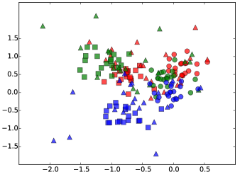
(a)

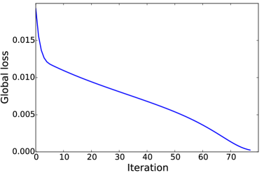
(b)

Figure 3: LABEL:sub@fig:synthetic_pts Artificial dataset for cross-entropy loss, with three domains (red, green and blue) and three categories (triangle, square, circle). LABEL:sub@fig:synthetic_loss_logloss Artificial dataset global loss versus iteration for cross-entropy loss. We empirically find that our solution converges to the global optimum of zero.

We next evaluate our algorithm on cross-entropy loss. Here we generate the two-dimensional dataset shown in Figure 3a, which has three domains, denoted in the colors red, green, and blue, and three categories, denoted as squares, circles, and triangles. Each domain is generated according to a Gaussian mixture model, one mixture per category, with random means. The means of each corresponding category across domains are related according to a random fixed orthonormal transformation. Finally, the covariance of each mixture is diagonal and fixed across categories. We choose covariance magnitudes of 0.05, 0.05, and 0.3 for the red, green, and blue domains, respectively. We then train a logistic regression classifier per domain to produce score functions, $h_{k}$. Finally, as the true distribution is known for this artificial example, we forgo density estimation and use the Gaussian mixture density function to generate our ${\mathscr{D}}_{k}$s.

With this data source, we use our DC-programming solution to find the optimal mixing weights, $z$. Since only each convex sub-problem is guaranteed to converge, Figure 3b reports this global loss vs iteration when initializing $z_{0}=1/p$, uniform weights. Here, the overall objective approaches 0.0, the known global minimum.To verify the robustness of the solution, we have experimented with various initial conditions and found the solution converges to the global solution from each case.

Table 5: MSE on sentiment analysis dataset: target domain as various combinations of two domains.

	Test Data
	KD	BE	KB	KE	DB	DE
K	1.83$\pm$0.08	1.99$\pm$0.10	1.87$\pm$0.08	1.57$\pm$0.06	2.25$\pm$0.08	1.94$\pm$0.10
D	1.95$\pm$0.07	2.11$\pm$0.07	2.12$\pm$0.07	2.11$\pm$0.05	1.95$\pm$0.06	1.94$\pm$0.06
B	2.10$\pm$0.09	1.99$\pm$0.08	1.96$\pm$0.07	2.21$\pm$0.06	1.87$\pm$0.07	2.13$\pm$0.05
E	2.00$\pm$0.09	1.95$\pm$0.07	2.05$\pm$0.05	1.60$\pm$0.05	2.36$\pm$0.07	1.91$\pm$0.07
unif	1.73$\pm$0.06	1.74$\pm$0.07	1.74$\pm$0.05	1.62$\pm$0.04	1.85$\pm$0.05	1.73$\pm$0.06
KMM	1.83$\pm$0.07	1.82$\pm$0.07	1.78$\pm$0.12	1.65$\pm$0.10	1.97$\pm$0.13	1.88$\pm$0.08
DW	1.62$\pm$0.07	1.61$\pm$0.08	1.59$\pm$0.05	1.47$\pm$0.04	1.75$\pm$0.05	1.64$\pm$0.05

Table 6: MSE on the sentiment analysis dataset: target domain as various mixture of four domains: $(\textbf{0.4},0.2,0.2,0.2)$, $(0.2,\textbf{0.4},0.2,0.2)$, $(0.2,0.2,\textbf{0.4},0.2)$, $(0.2,0.2,0.2,\textbf{0.4})$ of K, D, B, E respectively.

	Test Data
	KDBE	KDBE	KDBE	KDBE
K	1.78$\pm$0.05	1.94$\pm$0.10	1.96$\pm$0.08	1.84$\pm$0.07
D	2.02$\pm$0.10	1.98$\pm$0.10	2.06$\pm$0.11	2.05$\pm$0.09
B	2.01$\pm$0.12	2.01$\pm$0.14	1.94$\pm$0.14	2.06$\pm$0.11
E	1.93$\pm$0.08	2.04$\pm$0.10	2.08$\pm$0.10	1.89$\pm$0.08
unif	1.69$\pm$0.06	1.74$\pm$0.07	1.75$\pm$0.08	1.70$\pm$0.06
KMM	1.83$\pm$0.12	1.92$\pm$0.14	1.87$\pm$0.15	1.85$\pm$0.13
DW	1.55$\pm$0.08	1.62$\pm$0.08	1.59$\pm$0.09	1.56$\pm$0.08

Table 7: MSE on the sentiment analysis dataset: target domain as various mixture of four domains: $(\textbf{0.3},\textbf{0.3},0.2,0.2)$, $(\textbf{0.3},0.2,\textbf{0.3},0.2)$, $(\textbf{0.3},0.2,0.2,\textbf{0.3})$, $(0.2,\textbf{0.3},\textbf{0.3},0.2)$, $(0.2,\textbf{0.3},0.2,\textbf{0.3})$, $(0.2,0.2,\textbf{0.3},\textbf{0.3})$ of K, D, B, E respectively.

	Test Data
	KDBE	KDBE	KDBE	KDBE	KDBE	KDBE
K	1.86$\pm$0.10	1.87$\pm$0.07	1.79$\pm$0.08	1.96$\pm$0.10	1.89$\pm$0.10	1.89$\pm$0.08
D	2.01$\pm$0.13	2.05$\pm$0.12	2.04$\pm$0.12	2.03$\pm$0.12	2.02$\pm$0.13	2.06$\pm$0.12
B	2.01$\pm$0.15	1.98$\pm$0.14	2.05$\pm$0.13	1.98$\pm$0.15	2.04$\pm$0.14	2.01$\pm$0.13
E	2.00$\pm$0.10	2.01$\pm$0.09	1.91$\pm$0.08	2.08$\pm$0.10	1.97$\pm$0.08	1.99$\pm$0.08
unif	1.72$\pm$0.09	1.72$\pm$0.08	1.69$\pm$0.07	1.75$\pm$0.08	1.72$\pm$0.08	1.73$\pm$0.08
KMM	1.85$\pm$0.16	1.86$\pm$0.14	1.85$\pm$0.15	1.90$\pm$0.14	1.89$\pm$0.16	1.90$\pm$0.14
DW	1.58$\pm$0.10	1.57$\pm$0.10	1.55$\pm$0.09	1.61$\pm$0.10	1.59$\pm$0.08	1.58$\pm$0.09

E.2 Sentiment analysis task for squared loss

We begin by detailing our density estimation method for the sentiment analysis experiment. We first used the same vocabulary defined for feature extraction to train a separate bigram statistical language model for each domain, using the OpenGrm library (Roark et al., 2012). Next, we randomly draw a sample set $S_{k}$ of $10\mathord{,}000$ sentences from each bigram language model. We define $\widehat{\mathscr{D}}_{k}$ to be the empirical distribution of $S_{k}$, which is a very close estimate of marginal distribution of the language model, thus it is also a good estimate of ${\mathscr{D}}_{k}$. We approximate the label of a randomly generated sample $x_{i}$ by taking the average of the $h_{k}$s: $y_{i}=\sum_{\{k\colon x_{i}\in S_{k}\}}h_{k}(x_{i})/|\{k\colon x_{i}\in S_{k}\}|$. These randomly drawn samples were used to find the fixed-point $z$.

Note that we only use estimates of the marginal distributions (language models) to find $z$ and do not use any labels. We use the original product review text and rating labels for testing. Their densities $\widehat{\mathscr{D}}_{k}$ were estimated by the bigram language models directly, therefore a close estimate of ${\mathscr{D}}_{k}$.

Next we compare DW to accessible predictors on various test mixture domains. Table 5 shows MSE on all combinations of two domains. Table 6, 7 reports MSE on additional test mixture domains. The first four target mixtures correspond to various orderings of $(0.4,0.2,0.2,0.2)$. The next six target mixtures correspond to various orderings of $(0.3,0.3,0.2,0.2)$. In column titles we bold the domain(s) with highest weight.

In all these experiments, our distribution-weighted predictor DW outperforms all competing baselines: the source only baselines for each domain, K, D, B, E, a uniform weighted predictor unif, and KMM.

E.3 Recognition tasks for cross-entropy loss

Here, we describe our density estimation technique for the object recognition task.

To estimate the per domain densities, we first extract per image features using the in-domain ConvNet model, and then estimate the marginal distribution ${\mathscr{D}}^{1}_{k}(x)$ over the per domain collection of features, using non-parametric kernel density estimation with a Gaussian kernel and a cross-validated bandwidth parameter. We use estimated marginals $\widehat{\mathscr{D}}^{1}_{k}$ instead of estimated joint distributions $\widehat{\mathscr{D}}_{k}$, because when the conditional probabilities are the same across domains and when $\eta\to 0$, $h_{z}^{\eta}(x,y)$ converges to a normalized predictor $\widetilde{h}_{z}(x,y)=\sum_{k=1}^{p}\frac{z_{k}{\mathscr{D}}^{1}_{k}(x)}{\sum_{j=1}^{p}z_{j}{\mathscr{D}}^{1}_{j}(x)}h_{k}(x,y)$. Thus in our experiments, we approximate $\widehat{h}_{z}^{\eta}(x,y)$ with $\widetilde{\widehat{h}_{z}}(x,y)$ using our estimated marginal distributions $\widehat{\mathscr{D}}^{1}_{k}(x)$.

Appendix F Rényi Divergence

The Rényi Divergence measures the divergence between two distributions. The Rényi Divergence is parameterized by $\alpha$ and denoted by ${\mathsf{D}}_{\alpha}$. The $\alpha$-Rényi Divergence of two distributions ${\mathscr{D}}$ and ${\mathscr{D}}^{\prime}$ is defined by

$${\mathsf{D}}_{\alpha}({\mathscr{D}}\parallel{\mathscr{D}}^{\prime})=\frac{1}{\alpha-1}\log\sum_{(x,y)\in\mathcal{X}\times\mathcal{Y}}{\mathscr{D}}(x,y)\left[\frac{{\mathscr{D}}(x,y)}{{\mathscr{D}}^{\prime}(x,y)}\right]^{\alpha-1}.$$ (12)

It can be shown that the Rényi Divergence is always non-negative and that for any $\alpha>0$, ${\mathsf{D}}_{\alpha}({\mathscr{D}}\parallel{\mathscr{D}}^{\prime})=0$ iff ${\mathscr{D}}={\mathscr{D}}^{\prime}$, (see (Arndt, 2004)). We will denote by ${\mathsf{d}}_{\alpha}({\mathscr{D}}\parallel{\mathscr{D}}^{\prime})$ the exponential:

$${\mathsf{d}}_{\alpha}({\mathscr{D}}\parallel{\mathscr{D}}^{\prime})=e^{{\mathsf{D}}_{\alpha}({\mathscr{D}}\parallel{\mathscr{D}}^{\prime})}=\Bigg{[}\sum_{(x,y)\in\mathcal{X}\times\mathcal{Y}}\frac{{\mathscr{D}}^{\alpha}(x,y)}{{\mathscr{D}}^{\prime\alpha-1}(x,y)}\Bigg{]}^{\frac{1}{\alpha-1}}.$$ (13)

Rényi divergence (and ${\mathsf{d}}_{\alpha}({\mathscr{D}}\parallel{\mathscr{D}}^{\prime})$) is nondecreasing as a function of $\alpha$, and

$${\mathsf{d}}_{\alpha}({\mathscr{D}}\parallel{\mathscr{D}}^{\prime})\leq{\mathsf{d}}_{\infty}({\mathscr{D}}\parallel{\mathscr{D}}^{\prime})=\sup_{(x,y)\in\mathcal{X}\times\mathcal{Y}}\left[\frac{{\mathscr{D}}(x,y)}{{\mathscr{D}}^{\prime}(x,y)}\right].$$ (14)

References

• Arndt (2004) C. Arndt. Information Measures: Information and its Description in Science and Engineering. Signals and Communication Technology. Springer Verlag, 2004.
• Blitzer et al. (2007) J. Blitzer, M. Dredze, and F. Pereira. Biographies, bollywood, boom-boxes and blenders: Domain adaptation for sentiment classification. In Association for Computational Linguistics (ACL), 2007.
• Cover and Thomas (2006) T. M. Cover and J. M. Thomas. Elements of Information Theory. Wiley-Interscience, 2006.
• Donahue et al. (2014) J. Donahue, Y. Jia, O. Vinyals, J. Hoffman, N. Zhang, E. Tzeng, and T. Darrell. Decaf: A deep convolutional activation feature for generic visual recognition. In International Conference in Machine Learning (ICML), 2014.
• Dredze et al. (2008) M. Dredze, K. Crammer, and F. Pereira. Confidence-weighted linear classification. In International Conference on Machine Learning (ICML), 2008.
• Ganin and Lempitsky (2015) Y. Ganin and V. Lempitsky. Unsupervised domain adaptation by backpropagation. In International Conference in Machine Learning (ICML), 2015.
• Girshick et al. (2014) R. Girshick, J. Donahue, T. Darrell, and J. Malik. Rich feature hierarchies for accurate object detection and semantic segmentation. In In Proc. CVPR, 2014.
• Gong et al. (2012) B. Gong, Y. Shi, F. Sha, and K. Grauman. Geodesic flow kernel for unsupervised domain adaptation. In Proc. CVPR, 2012.
• Gong et al. (2013a) B. Gong, K. Grauman, and F. Sha. Connecting the dots with landmarks: Discriminatively learning domain-invariant features for unsupervised domain adaptation. In ICCV, 2013a.
• Gong et al. (2013b) B. Gong, K. Grauman, and F. Sha. Reshaping visual datasets for domain adaptation. In NIPS, 2013b.
• Hoffman et al. (2012) J. Hoffman, B. Kulis, T. Darrell, and K. Saenko. Discovering latent domains for multisource domain adaptation. In European Conference on Computer Vision (ECCV), 2012.
• Hoffman et al. (2013) J. Hoffman, E. Rodner, J. Donahue, K. Saenko, and T. Darrell. Efficient learning of domain-invariant image representations. In International Conference on Learning Representations, 2013.
• Huang et al. (2006) J. Huang, A. J. Smola, A. Gretton, K. M. Borgwardt, and B. Schölkopf. Correcting sample selection bias by unlabeled data. In Advances in Neural Information Processing Systems (NIPS), volume 19, pages 601–608, 2006.
• Krizhevsky et al. (2012) A. Krizhevsky, I. Sutskever, and G. E. Hinton. ImageNet classification with deep convolutional neural networks. In Proc. NIPS, 2012.
• Liao (2013) H. Liao. Speaker adaptation of context dependent deep neural networks. In ICASSP, 2013.
• Long et al. (2015) M. Long, Y. Cao, J. Wang, and M. I. Jordan. Learning transferable features with deep adaptation networks. In International Conference in Machine Learning (ICML), 2015.
• Mansour et al. (2008) Y. Mansour, M. Mohri, and A. Rostamizadeh. Domain adaptation with multiple sources. In NIPS, 2008.
• Mansour et al. (2009) Y. Mansour, M. Mohri, and A. Rostamizadeh. Multiple source adaptation and the Rényi divergence. In UAI, pages 367–374, 2009.
• Muandet et al. (2013) K. Muandet, D. Balduzzi, and B. Schölkopf. Domain generalization via invariant feature representation. In Proceedings of ICML, pages 10–18, 2013.
• Pan and Yang (2010) S. J. Pan and Q. Yang. A survey on transfer learning. In IEEE Transactions on Knowledge and Data Engineering, 2010.
• Rényi (1961) A. Rényi. On measures of entropy and information. In Proceedings of the Fourth Berkeley Symposium on Mathematical Statistics and Probability, volume 1, pages 547–561, 1961.
• Roark et al. (2012) B. Roark, R. Sproat, C. Allauzen, M. Riley, J. Sorensen, and T. Tai. The opengrm open-source finite-state grammar software libraries. In Proceedings of the ACL 2012 System Demonstrations, pages 61–66. Association for Computational Linguistics, 2012.
• Saenko et al. (2010) K. Saenko, B. Kulis, M. Fritz, and T. Darrell. Adapting visual category models to new domains. In Proc. ECCV, 2010.
• Sriperumbudur and Lanckriet (2012) B. K. Sriperumbudur and G. R. G. Lanckriet. A proof of convergence of the concave-convex procedure using Zangwill’s theory. Neural Computation, 24(6):1391–1407, 2012.
• Taigman et al. (2017) Y. Taigman, A. Polyak, and L. Wolf. Unsupervised cross-domain image generation. In International Conference on Learning Representations (ICLR), 2017.
• Tao and An (1997) P. D. Tao and L. T. H. An. Convex analysis approach to DC programming: theory, algorithms and applications. Acta Mathematica Vietnamica, 22(1):289–355, 1997.
• Tao and An (1998) P. D. Tao and L. T. H. An. A DC optimization algorithm for solving the trust-region subproblem. SIAM Journal on Optimization, 8(2):476–505, 1998.
• Torralba and Efros (2011) A. Torralba and A. Efros. Unbiased look at dataset bias. In CVPR, 2011.
• Tzeng et al. (2015) E. Tzeng, J. Hoffman, T. Darrell, and K. Saenko. Simultaneous deep transfer across domains and tasks. In International Conference in Computer Vision (ICCV), 2015.
• Xu et al. (2014) Z. Xu, W. Li, L. Niu, and D. Xu. Exploiting low-rank structure from latent domains for domain generalization. In European Conference in Computer Vision (ECCV), 2014.
• Yang et al. (2007) J. Yang, R. Yan, and A. G. Hauptmann. Cross-domain video concept detection using adaptive svms. ACM Multimedia, 2007.
• Yuille and Rangarajan (2003) A. L. Yuille and A. Rangarajan. The concave-convex procedure. Neural Computation, 15(4):915–936, 2003.
• Zhang et al. (2015) K. Zhang, M. Gong, and B. Schoelkopf. Multi-source domain adaptation: A causal view. In AAAI Conference on Artificial Intelligence, 2015.