End-to-End Refinement Guided by Pre-trained Prototypical Classifier

Abstract

Many real-world tasks involve identifying patterns from data satisfying background or prior knowledge. In domains like materials discovery, due to the flaws and biases in raw experimental data, the identification of X-ray diffraction patterns (XRD) often requires a huge amount of manual work in finding refined phases that are similar to the ideal theoretical ones. Automatically refining the raw XRDs utilizing the simulated theoretical data is thus desirable. We propose imitation refinement, a novel approach to refine imperfect input patterns, guided by a pre-trained classifier incorporating prior knowledge from simulated theoretical data, such that the refined patterns imitate the ideal data. The classifier is trained on the ideal simulated data to classify patterns and learns an embedding space where each class is represented by a prototype. The refiner learns to refine the imperfect patterns with small modifications, such that their embeddings are closer to the corresponding prototypes. We show that the refiner can be trained in both supervised and unsupervised fashions. We further illustrate the effectiveness of the proposed approach both qualitatively and quantitatively in a digit refinement task and an X-ray diffraction pattern refinement task in materials discovery.

Introduction

Many real-world tasks involve identifying meaningful patterns satisfying background or prior knowledge from limited amount of labeled data (?). Furthermore, the raw data are often corrupted with noise (?), which makes it even harder to identify meaningful patterns. On the other hand, in many domains like scientific discovery, though the experimental data might be flawed or biased, ideal data can often be synthesized easily (?; ?). It is thus desirable to incorporate knowledge from ideal data to refine the quality of the raw patterns to make them more meaningful and recognizable.

Figure 1: Imitation refinement improves the quality of imperfect patterns guided by a pre-trained classifier incorporating prior knowledge from ideal patterns. Left: Refinement of XRD patterns. Right: Refinement of hand-written digits.

For instance, in materials discovery, where we would like to discover new materials, each material is characterized by a unique X-ray diffraction pattern (also called XRD or phase, see Fig. 1). The identification of such phases is challenging because the raw phases from experiments are often mixed with each other and further corrupted with noise. Moreover, material scientists are interested in not only predicting the properties of materials (?), but also finding refined phases that are of better quality and similar to the ideal theoretical phases (?). To the best of our knowledge, this task can only be computed manually using quantum mechanics, which often requires huge amount of manual work even for an expert.

Even though our work has been motivated by applications in scientific discovery, there are other domains in which imitation refinement is applicable. For example, in the context of digit recognition, some scratchy hand-written digits may be hard to read since they may miss important strokes or are poorly written. Given the labels of the digits and synthesized “ideal” typeset digits, one may want to refine the hand-written digits to improve their readability, though typically we do not know what the corresponding ground-truth ideal digits are.

We propose a novel approach called imitation refinement, which improves the quality of imperfect patterns by imitating ideal patterns, guided by a classifier with prior knowledge pre-trained on the ideal dataset. Imitation refinement applies small modifications to the imperfect patterns such that (1) the refined patterns have better quality and are similar to the ideal patterns and (2) the pre-trained classifier can achieve better classification accuracy on the refined patterns. We show that both ends can be achieved even with limited amount of data.

Specifically, we pre-train a classifier using the ideal synthetic patterns and learn a meaningful embedding space. In such a space, each class forms a cluster containing all the embedded inputs from this class. We call the cluster centers prototypes for each class. Then the refiner learns a mapping from imperfect patterns to refined patterns, such that the embeddings of the refined patterns are closer to the corresponding prototypes and give better prediction results. In the supervised case, the corresponding prototype is the one associated with the class. In the unsupervised case, the prototype is the closest one to the raw embedded input.

The main contribution of our work is to provide a novel framework for imitation refinement, which can be used to improve the quality of imperfect patterns under the supervision from a classifier containing prior knowledge. Our second contribution is to find an effective way to incorporate the prior knowledge from the ideal data into the classifier. The third contribution of this work is to provide a way to train the refiner even if the imperfect inputs have no supervision.

Using a materials discovery dataset, we show that for the imperfect input experimental phases, the refined phases are closer to the quantum-mechanically computed ideal phases. In addition, we achieve higher classification accuracy on the refined phases. We show that even in the unsupervised case, the refinement can help improve the quality of the input patterns. To validate the generality of our approach, we also show that imitation refinement improves the quality of poorly written digits by imitating ideal typeset digits.

Imitation Refinement

Notation

In imitation refinement, we are given an ideal dataset $\mathcal{D}_{ideal}=\{(x_{i}^{ideal},y_{i}^{ideal})\}_{i=1}^{N}$. The ideal $d$-dimensional features $x_{i}^{ideal}\in\mathcal{X}^{ideal}\subseteq\mathbb{R}^{d}$ is a realization from a random variable $X^{ideal}$, and the label $y^{ideal}_{i}\in\mathcal{Y}$, where $\mathcal{Y}$ is a discrete set of classes $\{0,1,...,l\}$ in this problem. In addition, we are also given the imperfect training data $\mathcal{D}_{imp}$. In the supervised/targeted case, $\mathcal{D}_{imp}=\{(x^{imp}_{i},y^{imp}_{i})\}_{i=1}^{M}$ where $x_{i}^{imp}\in\mathcal{X}^{imp}\subseteq\mathbb{R}^{d}$ is a realization of a random variable $X^{imp}$ and the labels $y^{imp}_{i}\in\mathcal{Y}$. In the unsupervised/non-targeted case, $\mathcal{D}_{imp}=\{x^{imp}_{i}\}_{i=1}^{M}$ where $x^{imp}\in\mathcal{X}^{imp}$ and the labels are not available. We assume there is a slight difference (?; ?) between $\mathcal{X}^{imp}$ and $\mathcal{X}^{ideal}$.

Problem Description

Our goal is to learn a function $\mathcal{R}:\mathcal{X}^{imp}\to\mathcal{X}^{rfd}$, where $\mathcal{X}^{rfd}\subseteq\mathcal{X}^{ideal},$ that refines the imperfect patterns into ideal patterns (e.g. the theoretically computed corresponding patterns), with the guidance from a pre-trained classifier $\mathcal{C}$. $\mathcal{C}$ is the composition $\mathcal{G}_{\psi}\circ\mathcal{F}_{\theta}$ where $\mathcal{F}_{\theta}:\mathcal{X}^{ideal}\to\mathbb{R}^{m}$ is an embedding function ($m$-dimensional embedding space) and $\mathcal{G}_{\psi}:\mathbb{R}^{m}\to\mathcal{Y}$ is a prediction function. For the inputs $x$, we hope $\mathcal{C}(\mathcal{R}(x))$ can give better results than $\mathcal{C}(x)$, and $\mathcal{R}(x)$ has better quality than $x$, by imitating the patterns in $\mathcal{X}^{ideal}$.

Pre-trained Prototypical Classifier

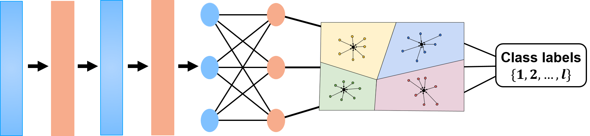
Figure 2: Prototypical classifier not only predicts labels, but also learn a meaningful embedding space. The center of the cluster for each class is called prototype.

Inspired by recently proposed prototypical networks (?), the classifier is trained to learn a meaningful embedding space to better incorporate the prior knowledge as well as the class prediction. The embedding space is formed by the features from the last layer before the softmax layer, where each class can be represented by a prototype embedding and embeddings from each class form a cluster surrounding the prototype. We thus call the classifier prototypical classifier. The ideal dataset is used to train the prototypical classifier and inject prior knowledge into the classifier. The prototype of each class is the mean of the embedded patterns from this class:

$$c_{k}=\frac{1}{|\mathcal{D}^{ideal}_{k}|}\sum_{y_{i}^{ideal}=k}\mathcal{F}_{\theta}(x_{i}^{ideal})$$ (1)

where $c_{k}$ is the prototype of class $k$ and $\mathcal{D}^{ideal}_{k}$ is the subset of $\mathcal{D}_{ideal}$ containing all the samples from class $k$.

To learn such a prototypical classifier, besides the class prediction loss given by a classification loss $\mathcal{L}_{\mathcal{C}}(\theta,\psi)=\sum_{i}\ell(\mathcal{G}_{\psi}(\mathcal{F}_{\theta}(x^{ideal}_{i})),y_{i}^{ideal})$ where $\ell(\cdot)$ can be the cross entropy loss or other supervised losses, we further add a loss defining the distances to the ground-truth prototypes in the embedding space given a distance function $d:\mathbb{R}^{m}\times\mathbb{R}^{m}\to[0,+\infty)$:

$$\mathcal{L}_{\mathcal{F}}(\theta)=\sum_{i}-\log\frac{\exp(-d(\mathcal{F}_{\theta}(x_{i}^{ideal}),c_{y_{i}^{ideal}}))}{\sum_{k^{\prime}\in\mathcal{Y}}\exp(-d(\mathcal{F}_{\theta}(x_{i}^{ideal}),c_{k^{\prime}}))}$$ (2)

The idea behind this loss is simple: for a sample $x_{i}^{ideal}$, we define a distribution over classes based on a softmax over the distances to the prototypes and the loss is simply the negative log-likelihood of the probabilities. In each training step, the batch of samples are randomly selected from each class to ensure each class has a least one sample. The prototype of each class is randomly initialized before the training and is updated by computing the mean of the embeddings from the class and the prototype from last batch. During the training, we also consider the prototypes from the last batch while updating the prototypes to stabilize the prototypes instead of learning new prototypes in each step. If we assume the embedding space is well formed by clusters (which will be shown in experimental section), cluster means are the best representatives as shown in (?). Pseudocode to train the prototypical classifier is provided in Algorithm 1. Fig. 2 gives an overview of the prototypical classifier.

Algorithm 1 One epoch in the training for the prototypical classifier

Input: Ideal dataset $\mathcal{D}_{ideal}=\{(x_{i}^{ideal},y_{i}^{ideal})\}_{i=1}^{N}$ where $y_{i}^{ideal}\in\{1,...,l\}$, max number of batches($T$), the number of samples selected from each class in each step($N_{c}$), the subset $\mathcal{D}_{k}$ containing all the samples from class $k$.
Output: Prototypical classifier $\mathcal{C}_{\theta,\psi}$.

1:Randomly initialize prototypes $c^{0}_{k}$ for each class.

2:for $t=1,...,T$ do

3:     for $k=1,...,l$ do

4:         Randomly select $N_{c}$ samples from class $k$.      

5:     Compute $\mathcal{L}_{\mathcal{C}}(\theta,\psi)$ and $\mathcal{L}_{\mathcal{F}}(\theta)$ given the samples and prototypes.

6:     $\mathcal{L}_{batch}(\theta,\psi)\leftarrow\mathcal{L}_{\mathcal{C}}(\theta,\psi)+\lambda\mathcal{L}_{\mathcal{F}}(\theta)$.

7:     Update the parameters $\theta,\psi$ by taking an Adam step on the batch loss.

8:     $c_{k}^{t}\leftarrow\frac{1}{|\mathcal{D}^{ideal}_{k}|+1}(c^{t-1}_{k}+\sum_{y_{i}^{ideal}=k}\mathcal{F}_{\theta}(x_{i}^{ideal}))$

Imitation Refiner

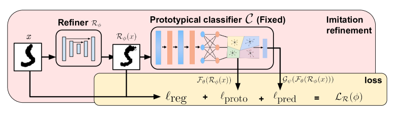
Figure 3: The refiner $\mathcal{R}_{\phi}$ is trained in an end-to-end fashion. The Pre-trained classifier $\mathcal{C}$ provides two losses, $\ell_{\mbox{proto}}$ and $\ell_{\mbox{pred}}$. Loss $\ell_{\mbox{reg}}$ is given by the difference between the refined input and the raw input in either the raw space or some feature space.

The pre-trained prototypical classifier is then applied to guide the training of the refiner $\mathcal{R}_{\phi}:\mathcal{X}^{imp}\to\mathcal{X}^{rfd}$ with learnable parameters $\phi$. We propose to learn $\phi$ by minimizing a combination of three losses:

$$\mathcal{L}_{R}(\phi)= \sum_{i}(\ell_{\mbox{pred}}(\phi;x_{i}^{imp},\mathcal{Y})+\alpha\ell_{\mbox{reg}}(\phi;x_{i}^{imp})$$ (3)

$$+\beta\ell_{\mbox{proto}}(\phi;x_{i}^{imp},\mathcal{F}(\mathcal{X}^{ideal}))).$$

where $x_{i}^{imp}$ is the $i^{th}$ imperfect training sample and $\mathcal{F}(\mathcal{X}^{ideal})$ is the embedding space formed by the embeddings of samples from the space $\mathcal{X}^{ideal}$. $\alpha$ and $\beta$ are coefficients that trade off different losses. Note that once the classifier $\mathcal{C}$ is trained, it is fixed along with the prototypes $c_{k}$’s during the training of the refiner. Furthermore, $\mathcal{C}$ provides loss functions ($\ell_{\mbox{pred}}$ and $\ell_{\mbox{proto}}$) to the training of $\mathcal{R}_{\phi}$.

As we mentioned previously, the refiner can be trained in both targeted and non-targeted fashions, depending on whether the labels of the imperfect training samples are provided or not. In the targeted case, prediction loss $\ell_{\mbox{pred}}$ is the loss given by the difference between the predicted labels of the refined input patterns and the ground-truth labels:

$$\ell_{\mbox{pred}}(\phi;x_{i}^{imp},\mathcal{Y})=\mathcal{H}(\mathcal{C}(\mathcal{R}_{\phi}(x_{i}^{imp})),y_{i}^{imp})$$ (4)

where $\mathcal{H}$ is the cross-entropy loss. In the non-targeted case, we simply change the cross-entropy loss to the entropy loss, $\mathcal{H}(\mathcal{C}(\mathcal{R}_{\phi}(x_{i}^{imp})))$, to represent the uncertainty of the classifier $\mathcal{C}$ on the refined patterns. The goal is to minimize the entropy to force the refiner to learn more meaningful refined patterns which could be better recognized by $\mathcal{C}$.

Simply using the prediction loss is not sufficient to learn an effective refiner and sometime might learn adversarial examples (?). We thus introduce the prototypical loss $\ell_{\mbox{proto}}$ to further guide the refinement towards the corresponding prototypes in the embedding space, which is more robust. In the targeted case, the prototypical loss is given by the negative log-likelihood on the distances between the embeddings of the refined patterns and the ground-truth prototypes:

$$\ell_{\mbox{proto}}(\phi;x_{i}^{imp},\mathcal{F}(\mathcal{X}^{ideal}))$$ (5)

$$= -\log\frac{\exp(-d(\mathcal{F}(\mathcal{R}_{\phi}(x_{i}^{imp})),c_{y_{i}^{imp}}))}{\sum_{k^{\prime}}\exp(-d(\mathcal{F}(\mathcal{R}_{\phi}(x_{i}^{imp})),c_{k^{\prime}}))}$$

In the non-targeted case, we use entropy loss:

$$\ell_{\mbox{proto}}(\phi;x_{i}^{imp},\mathcal{F}(\mathcal{X}^{ideal}))=\sum_{k=1}^{l}-p^{imp}_{i,k}\log{p^{imp}_{i,k}}$$ (6)

where $p_{i,k}^{imp}=\frac{\exp(-d(\mathcal{F}(\mathcal{R}_{\phi}(x_{i}^{imp})),c_{k}))}{\sum_{k^{\prime}}\exp(-d(\mathcal{F}(\mathcal{R}_{\phi}(x_{i}^{imp})),c_{k^{\prime}}))}$.

Algorithm 2 One epoch in the training for the refiner when labels are available

Input: Imperfect training dataset $\mathcal{D}_{imp}=\{(x_{i}^{imp},y_{i}^{imp})\}_{i=1}^{M}$ where $y_{i}^{imp}\in\{1,...,l\}$, max number of batches($T$), the batch size($N_{c}$), the prototypical classifier $\mathcal{C}$ and the prototypes $c_{k}$.
Output: Refiner $\mathcal{R}_{\phi}$.

1:for t=1..T do

2:     Sample $N_{c}$ samples from training set $D_{imp}:\{x_{i},y_{i}\}_{i=1}^{N_{c}}$.

3:     Let $r_{i}=\mathcal{R}(x_{i})$ be the refined inputs.

4:     Let $e_{i}=\mathcal{F}(r_{i})$ be the embedded refined inputs.

5:     Let $c_{i}=\mathcal{G}(e_{i})$ be the predicted labels.

6:     Compute $\mathcal{L}_{\mathcal{R}}(\phi)$ in equation (3)

• $\ell_{\mbox{pred}}=\frac{1}{N_{c}}\sum_{i}\mathcal{H}(c_{i},y_{i})$

• $\ell_{\mbox{proto}}=\frac{1}{N_{c}}\sum_{i}-\log\frac{\exp(-d(e_{i},c_{y_{i}}))}{\sum_{k^{\prime}}\exp(-d(e_{i},c_{k^{\prime}}))}$

• $\ell_{\mbox{reg}}=\frac{1}{N_{c}}\sum_{i}||\Psi(r_{i})-\Psi(x_{i})||_{p}$

7:     Update parameters $\phi$ through back-propagation based on the loss $\mathcal{L}_{\mathcal{R}}(\phi)$.

Note that for an imperfect sample $x_{i}^{imp}$, we are looking for an ideal pattern in $\mathcal{X}^{ideal}$ that is most related to $x_{i}^{imp}$. $\mathcal{R}$ should modify the input as little as possible to remain the contents in the imperfect input samples (?). Therefore, we introduce the third loss $\ell_{\mbox{reg}}$ to regularize the changes made for the input:

$$\ell_{\mbox{reg}}(\phi;x^{imp}_{i})=||\Psi(\mathcal{R}(x_{i}^{imp}))-\Psi(x_{i}^{imp})||_{p}$$ (7)

where $||\cdot||_{p}$ is p-norm and $\Psi$ maps the raw input into a feature space. $\Psi$ can be an identity map $\Psi(x)=x$ or more abstract features such as the feature maps after the first or second convolution layer. This loss works for both targeted and non-targeted cases since it does not rely on the labels. Such regularization can also help avoid learning an ill-posed mapping from $\mathcal{X}^{imp}$ to $\mathcal{X}^{ideal}$ such as a many-to-one mapping that maps all the imperfect patterns from class $k$ to one ideal pattern in class $k$ regardless the raw contents in the imperfect patterns. This mapping could achieve very small $\ell_{\mbox{pred}}$ and $\ell_{\mbox{proto}}$ but that is not what we want.

The refiner $\mathcal{R}$ is trained in an end-to-end way as described above and all the parameters are updated through back-propagation. The pseudocode to train the refiner is provided in Algorithm 2 in the targeted case. In the non-targeted case, the algorithm is simply replacing the targeted losses with non-targeted losses as described. The overall structure of the refiner is shown in Fig. 3.

Experiments

In this section we present results to validate our approach on two applications: materials discovery (?) and hand-written digits refinement (?).

Materials Discovery

High-throughput combinatorial materials discovery is a materials science task whose intent is to discover new materials using a variety of methods including X-ray diffraction pattern analysis(?). The raw imperfect X-ray diffraction patterns (XRD) from experiments are often unsatisfiable because the data corruption could happen in any step of the data processing. Much effort has been put into cleaning the data through techniques like matrix decomposition, data smoothing (?; ?). These previous works mainly focus on individual pattern cleaning instead of modifying the pattern by considering prior knowledge. Thus, experts still need to do considerable manual work to fit the data into the heavy-duty quantum mechanical computation to find a refined XRD similar to some perfect theoretical pattern, which may take weeks or even months. However, some domain knowledge can be very useful to automatically push the refinement of the imperfect XRD patterns. For example, it is a fundamental fact that each XRD could be categorized as exactly 1 of the 7 crystal structures (triclinic, monoclinic, orthorhombic, tetragonal, rhombohedral, hexagonal, cubic). Each structure has some unique signal patterns. We want to learn such knowledge from the ideally simulated data and further guide the refinement of the imperfect XRD patterns.

In this work, we show how close the refined XRDs are to the quantum-mechanically computed patterns to validate that useful domain knowledge is learned by the pre-trained classifier. We show our performance via two metrics. First, the refined XRDs can achieve better classification accuracy even if the classifier is not changed. Second, we directly show the improvement of the quality of the refined XRDs both qualitatively and quantitatively. We measure the difference between the ground-truth XRDs and refined XRDs on $\ell_{1},\ell_{2}$, KL-divergence and cross correlation. Qualitative results are also shown in the heatmaps of the XRDs.

Dataset: The dataset used in this application is from materials project (?). The ideal simulated data have approximately 240,000 samples from 7 classes. Each sample is a 2,000-dimensional 1-d feature. The label of each ideal sample is also known. This dataset is not balanced where the trilinic class has as few as 14,000 samples while the cubic class has over 52,000 samples. Such data imbalance can be handled by the batch selection strategy in the training for the prototypical classifier. The imperfect dataset has only 1,494 samples from 7 classes, which is much fewer than the ideal dataset. 5-fold cross-validation is used for training the classifier and refiner. Furthermore, the theoretically computed ground-truth XRDs from materials scientist are also provided and are only used for evaluation purpose. For training the refiner, we have two settings where the class labels may or may not be known.

Implementation details: The refiner network, $\mathcal{R}_{\phi}$ is U-Net (?). Since the inputs are 1-d XRD patterns of length 2000, all the 2-d layers in the U-Net are changed to 1-d layer while other configurations remain the same. The input $2000\times 1$ feature is convolved with $3\times 1$ filters that output 32 feature maps. The output is then passed through an encoder-decoder network structure with 4 convolutional and 4 deconvolutional layers. The output of the last layer passes through a $1\times 1$ convolutional layer which produces 1 feature map of size $2000\times 1$.

For the classifier $\mathcal{C}$, we use two structures DenseNet (?) and VGG (?) to show that the imitation refinement framework works for different classifiers. For DenseNet, DenseNet-121 structuere is adopted, with 4 blocks where the numbers of dense-layers in each block are 6, 12, 24, 16. Each dense-layer is a composition of two BatchNorm-ReLU-Conv layers where the filter size is $5\times 1$. Growth rate is set to be 32. Note that the input pattern would go through Conv-BatchNorm-ReLU-Pooling layers first to produce a feature map that can be fed into subsequent blocks. VGG-19 is another classifier used in our experiments. We keep most configurations from the original paper except that all the 2-d layers are adapted to 1-d layers. The kernel size for the convolutional layers is $3\times 1$ and the kernel size for the max pooling layers is $10\times 1$. These changes are only made to fit the dimensionality of the input XRDs. In this application, function $\mathcal{G}$ is the last softmax layer of the classifier and $\mathcal{F}$ is the rest part of the classifier outputing the embeddings. We train the prototypical classifier for 100 epochs with batch size 512 (73 from each class and 1 more cubic to get sum 512). Function $\Psi(\cdot)$ is identity function and $\ell_{\mbox{reg}}$ uses $\ell_{1}$ norm. We use Adam to train the classifier with learning rate 0.001.

Models	Standard	Prototypical
VGG-19	68.54%	69.01%
DenseNet	67.74%	70.82%

Table 1: XRD patterns: A classifier pre-trained on the ideal dataset is tested on the imperfect data. The accuracies from standard and prototypical classifiers are given in the table. Prototypical classifiers perform better that the standard classifiers. These results are also used as baselines.

We first show the advantage of the prototypical classifier over the standard classifier with regard to the generalization by directly feeding the imperfect data into the classifiers pre-trained on the ideal dataset. Table 1 shows the results. These results also serve as the baselines.

Models	Accuracy
DWT	71.28%
ADDA	73.78%
GTA	73.18%
UNet+VGG	71.37%
UNet+proto-VGG	73.98%
UNet+DenseNet	76.50%
UNet+proto-DenseNet	80.05%
non-targeted UNet+proto-VGG	71.63%
non-targeted UNet+proto-DenseNet	74.74%

Table 2: Different accuracies from different methods or different settings. We also give the results in non-targeted cases. Our method outperforms the previous methods.

To show the improvement of the refined inputs with regard to the classification performance, Table 2 presents the label prediction accuracies from different methods or settings. Discrete wavelet transform (?) is a widely used signal denoising technique in materials science domain. It removes high frequency noise and produces cleaner data. ADDA (?) is a recently proposed adversarial domain adaptation method aiming at learning different feature extraction networks for two similar domains. The embedding space learned by the two networks are aligned and can be used to predict labels. GTA (?) also learns a common embedding space that can be used for class prediction, as well as for training a GAN (?) where the generator acts as a decoder decoding the embedding to a pattern in the raw feature space. The decoded pattern is then fed into a multi-class discriminator. As shown in the table, our methods outperform these state-of-art methods in this application where the imperfect data is not abundant. This table also shows that the refinement using the prototypical classifiers can achieve better results than using standard classifiers. The strength of our method when the labels are not available (non-targeted case) is demonstrated in the table as well. Compared to the two baselines ($69.01\%$ and $70.82\%$), the unsupervised training under the proposed framework gives promising results (71.63% and 74.74%).

Ablation study: To show the combination of the different losses is necessary and meaningful, we show the results in Table 3 when either $\ell_{\mbox{proto}}$ or $\ell_{\mbox{pred}}$ is ablated. Note that all the reported numbers are averaged over 5 independent runs.

Models	$\ell_{\mbox{proto}}$	$\ell_{\mbox{pred}}$	$\ell_{\mbox{reg}}$	Accuracy
UNet+DenseNet	Y	N	Y	79.33%
UNet+DenseNet	N	Y	Y	75.76%
UNet+DenseNet	Y	Y	Y	80.05%

Table 3: The combination of 3 losses gives the best accuracy. “Y” stands for yes and “N” stands for no.

Quantitative results With respect to the quality of refined XRDs: We directly measure the differences between the refined XRDs and the ground-truth theoretical XRDs on 4 metrics, $\ell_{1},\ell_{2}$, kl-divergence and cross correlation. We compute both the averages and the medians of the differences over all the test data (Table 4). ADDA cannot produce refined XRDs, so it is skipped in this part of experiment. GTA does not perform well in the quality measurement since it does not consider the self-regularization loss or a prototypical loss and it actually learns a different refinement space. Besides, the embedding space learned by GTA is not as well-formed as imitation refinement (see Fig. 4).

Qualitative analysis: Fig. 4 gives a comparison between the embedding space learned by GTA and imitation refinement. Fig. 5 gives an example of the raw XRD, refined XRD and the ground-truth XRD for materials NbGa₃ and Mn₄Al₁₁.

(a) GTA embedding space

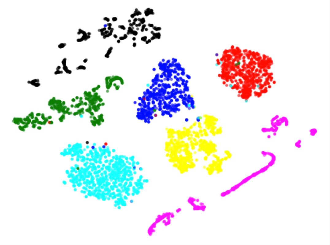
(b) Our embedding space

Figure 4: TSNE visualization of the embedding spaces learned by GTA and our imitation refinement. Each color represents a class. The embedding space from our method clusters the data better.

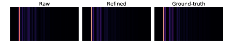
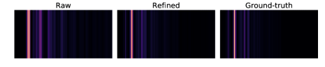
Figure 5: The visualization of the raw, refined and ground-truth XRDs for NbGa₃ and Mn₄Al₁₁ (best in color). The first one originally has 3 dim high peaks instead of 1 bright peak as in the ground-truth. Our method successfully squeezes the 3 peaks into one brightest peak. The second one originally does not have 3 peaks on the left to the brightest peak as ground-truth. Imitation refinement adds them.

	Average				Median
Models	$\ell_{1}$	$\ell_{2}$	$KL$	NCC	$\ell_{1}$	$\ell_{2}$	$KL$	NCC
Raw XRD	38.993	4.913	41.027	24.415	26.749	1.718	12.195	20.870
DWT	37.459	4.722	37.920	24.305	25.642	1.706	11.972	20.884
GTA	89.265	9.498	48.263	20.991	90.914	6.861	23.306	20.618
UNet+proto-VGG	37.709	4.822	35.750	24.514	26.200	1.603	11.686	20.956
non-targeted UNet+proto-VGG	38.843	4.983	38.494	24.205	26.034	1.630	12.545	21.232
UNet+proto-DenseNet	36.744	4.382	31.767	25.827	25.101	1.671	11.945	22.481
non-targeted UNet+proto-DenseNet	37.119	4.797	36.246	24.364	27.235	1.754	11.834	21.079

Table 4: Differences between the refined XRDs and the ground-truth XRDs on metrics $\ell_{1},\ell_{2},KL$ and normalized cross correlation (NCC). The difference between the raw XRDs and the ground-truth XRDs gives the baseline. The differences shown in the table are the averages or medians over all the test data. For $\ell_{1},\ell_{2},kl$, the smaller the better. For NCC, the larger, the better. The best results for each measure is in bold.

Hand-Written Digits

We also show the generality of our model in a hand-written digit refinement task. In this experiment, we show that if the ideal digits typeset in different fonts are given, imitation refinement can take advantage of these ideal digits to refine handwritten digits, so as to improve prediction accuracy as well as the readability.

Ideal Digit Datasets: We generate an ideal dataset containing images of digits typeset in five different fonts respectively: $\mathtt{Bradly~{}Hand}$, $\mathtt{Brush~{}Script}$, $\mathtt{Hannotate}$, $\mathtt{Times}$, and $\mathtt{Typewriter}$. We augment images in each font by vertically and horizontally shifting at most two pixels, and also rotating in range $[-20^{\circ},20^{\circ}]$. Each dataset contains 10250 images of digits. We merge these five datasets to a dataset $\mathtt{Synz}$ containing these synthetic digits.

Handwritten Digit Datasets: The MNIST dataset (?) is used as our imperfect dataset, which contains 60,000 handwritten digits for the training and validation and another 10,000 digits for testing. Some examples of digits in the ideal dataset and imperfect dataset are shown in Fig. 6. Our goal is to refine handwritten digits by mimicking the characteristics of computer generated fonts. We take 1 to 50 examples from each class to produce a small training set (10 to 500 data in total), which is then used for training. To allow reproducibility and reduce randomness in sparse data selection, we select first $N$ ($N\in\{1,2,5,10,20,30,40,50\}$) data in each class of the official MNIST training dataset. This dataset imitates data obtained under scenarios in which labeled data can be only sparsely obtained.

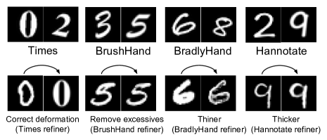
Figure 6: The first row displays example digits in the ideal dataset. The second row shows examples of imitatively refining MNIST handwritten digits to have the characteristics of different fonts.

Implementation details Most experimental settings remain the same as the previous materials discovery application except that the batch size in training the classifier is 100 and the optimizer is RMSprop with learning rate 0.01.

We first train the prototypical classifier $\mathcal{C}$ on the ideal digit datasets. $\mathcal{C}$ classifies instances in the ideal dataset into 10 categories (0-9). Similar to the earlier experiment, we take DenseNet-121 as the basic network structure. In order to fit the smaller resolution input of this experiment, we replaced the first downsampling convolution with a convolution of stride 1, and we remove the first max-pooling layer and the first dense block. The rest remains unchanged. This classifier achieves over $99.9\%$ test accuracy on the ideal datasets.

We use a U-Net structured model as the refiner on the MNIST dataset. Note this network is very small, with only 60k parameters (compared to 900k parameters in DenseNet). Therefore adding very little overhead to the existing classifier. When training, we consider two cases: a targeted case in which the labels of handwritten digits are given and a non-target case where the labels are not given. Note that in both cases, the ideal counterparts of the imperfect digits are unknown. By training our network end-to-end, the network is able to learn how to best perform this refinement. This will be shown quantitatively in the next section.

Improvement of accuracy:

As mentioned previously, we take 1 to 50 examples from each class to produce a small training set (0.02%-1% of entire MNIST training dataset). Fig. 7 shows the improvement of identifiability of hand-written digits after imitation refinement.

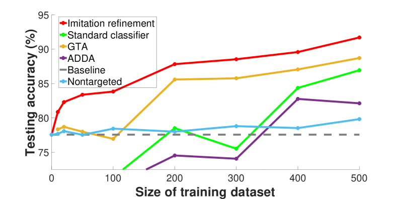
Figure 7: As the number of training examples from MNIST dataset increases, the test accuracies of all the methods can increase gradually. However, only imitation refinement consistently outperforms the baseline and other methods.

The baseline is given in the gray dash line. Directly feeding the mnist test data into the pre-trained prototypical classifier gives an accuracy of 77.57%. This result is better than the accuracy obtained when using a standard classifier with the same structure, which is only 70.26%. The green line is achieved by training a standard classifier from scratch on the very few given training data from scratch. When the number of samples from each class is smaller than 10, the classifier cannot learn anything. But as the number of training samples grows, the accuracy also increases. This classifier cannot outperform the baseline stably until after seeing over 40 samples from each class. The results given by another two compared methods, ADDA and GTA are also shown here. ADDA corresponds to the purple line and its performance is not very promising in this scarce data scenario. GTA performs better in that it learns a more meaningful embedding space which helps the classification even when the data amount is not rich. The results of imitation refinement are given by the red line. Starting from the baseline accuracy, imitation refinement consistently outperforms the other methods and it improves with the increase of training dataset size. Note that imitation refinement obtains better results by modifying and refining the classifier’s input, instead of changing the classifier’s model. This illustrates that the prior knowledge learned by the classifier can actually help produce meaningful refined patterns and is a key difference between our work and related methods such as transfer learning. Fig. 6 also shows the meaningful features learned in the refined digits. For instance, “0” learns a meaningful deformation to mimic the $\mathtt{Times}$ style and “1” learns the essential bottom bar in the refined digit while preserving most contents in the raw image. We also perform imitation refinement in the non-targeted case and it outperforms the baseline and increases the baseline accuracy with a margin of over 2% when 50 samples are given per class.

Related Work

Imitation refinement is related to data denoising (?) and data restoration (?), which improve noisy or corrupted data. One key difference is that imitation refinement does not require imperfect data to be paired with its cleaned version while training. We directly train an imitation refiner on the imperfect dataset, for which we don’t know the ground truth. Also, the ideal dataset does not provide ground truth counterparts for the imperfect data. Our work is also related to style transfer (?), which requires paired images or cycle consistency (a bijection between two domains) for the transformation. Besides, transfer learning (?) and domain adaptation (?) modify models while our classifier is fixed. Additionally, imitation refinement has notable differences with conventional inverse classification (?; ?), which uses inverted statistics to complete partial data or solve an optimization problem for each test sample respectively. Imitation refinement differs from these methods since it incorporates the knowledge embedded in a pre-trained classifier into the refiner, which can generalize to the unseen imperfect data. Further, imitation refinement allows for high-level data modification, while inverse classification often only changes data attributes. Finally, imitation refinement is different from GAN (?) since its goal is not to refine imperfect data such that a discriminator cannot differentiate them from ideal data. Instead, imitation refinement only applies small modifications to the imperfect data to reflect the fundamental characteristics of the ideal data, captured by the classifier trained on them. Several recently proposed domain adaptation methods using GAN (?; ?) seek to find a common space for both target domain and source domain. Though they give nice classification results, the performance on the refinement of the raw inputs is not their focus. Besides, these methods typically require a certain amount of data. As shown in the experimental section, they do not perform very well when only a limited amount of imperfect training data are given. Prototypical network (?) is closely related to our work. It learns a meaningful embedding space formed by the support sets from each batch. However, their work use the embedding space for classification while we mainly use it for refinement.

Conclusion and Future Work

Imitation refinement improves the quality of imperfect data by imitating ideal data. Using the prior knowledge captured by a prototypical classifier trained on an ideal dataset, a refiner learns to apply modifications to imperfect data to improve their qualities. A general end-to-end neural framework is proposed to address this refinement task and gives promising results in two applications: handwritten digits and XRD pattern refinement. Imitation refinement improves readability and accuracy of identifying handwritten digits and refines the XRDs to be closer to the ground-truth patterns. This work has a potential to save lots of manual work for material scientists. We also show that imitation refinement could work even if labels are not provided. Imitation refinement is easily adaptable to other different situations, such as crowd-sourcing tasks, where the raw data are often imperfect. The refiner and classifier are also replaceable components and we have shown that the imitation refinement framework can incorporate prior knowledge efficiently. We hope our work will stimulate additional imitation refinement efforts.

References

- [Aggarwal, Chen, and Han 2010] Aggarwal, C. C.; Chen, C.; and Han, J. 2010. The inverse classification problem. Journal of Computer Science and Technology 25(3):458–468.
- [Banerjee et al. 2005] Banerjee, A.; Merugu, S.; Dhillon, I. S.; and Ghosh, J. 2005. Clustering with bregman divergences. Journal of machine learning research 6(Oct):1705–1749.
- [Cai and Harrington 1998] Cai, C., and Harrington, P. d. B. 1998. Different discrete wavelet transforms applied to denoising analytical data. Journal of chemical information and computer sciences 38(6):1161–1170.
- [Chapelle, Scholkopf, and Zien 2009] Chapelle, O.; Scholkopf, B.; and Zien, A. 2009. Semi-supervised learning. IEEE Transactions on Neural Networks 20(3):542–542.
- [Chen et al. 2005] Chen, Z. P.; Morris, J.; Martin, E.; Hammond, R. B.; Lai, X.; Ma, C.; Purba, E.; Roberts, K. J.; and Bytheway, R. 2005. Enhancing the signal-to-noise ratio of x-ray diffraction profiles by smoothed principal component analysis. Analytical chemistry 77(20):6563–6570.
- [Dong et al. 2014] Dong, C.; Loy, C. C.; He, K.; and Tang, X. 2014. Learning a deep convolutional network for image super-resolution. In European Conference on Computer Vision. Springer.
- [Gatys, Ecker, and Bethge 2016] Gatys, L. A.; Ecker, A. S.; and Bethge, M. 2016. Image style transfer using convolutional neural networks. In Proceedings of the IEEE Conference on Computer Vision and Pattern Recognition, 2414–2423.
- [Glorot, Bordes, and Bengio 2011] Glorot, X.; Bordes, A.; and Bengio, Y. 2011. Domain adaptation for large-scale sentiment classification: A deep learning approach. In Proceedings of the 28th international conference on machine learning, 513–520.
- [Goodfellow et al. 2014] Goodfellow, I.; Pouget-Abadie, J.; Mirza, M.; Xu, B.; Warde-Farley, D.; Ozair, S.; Courville, A.; and Bengio, Y. 2014. Generative adversarial nets. In Advances in neural information processing systems, 2672–2680.
- [Green et al. 2017] Green, M. L.; Choi, C.; Hattrick-Simpers, J.; Joshi, A.; Takeuchi, I.; Barron, S.; Campo, E.; Chiang, T.; Empedocles, S.; Gregoire, J.; et al. 2017. Fulfilling the promise of the materials genome initiative with high-throughput experimental methodologies. Applied Physics Reviews 4(1):011105.
- [Huang et al. 2017] Huang, G.; Liu, Z.; van der Maaten, L.; and Weinberger, K. Q. 2017. Densely connected convolutional networks.
- [Jain et al. 2013] Jain, A.; Ong, S. P.; Hautier, G.; Chen, W.; Richards, W. D.; Dacek, S.; Cholia, S.; Gunter, D.; Skinner, D.; Ceder, G.; et al. 2013. Commentary: The materials project: A materials genome approach to accelerating materials innovation. Apl Materials 1(1):011002.
- [Kurakin, Goodfellow, and Bengio 2016] Kurakin, A.; Goodfellow, I.; and Bengio, S. 2016. Adversarial examples in the physical world. arXiv preprint arXiv:1607.02533.
- [Le Bras et al. 2014] Le Bras, R.; Bernstein, R.; Suram, J. M.; Gregoire, S. K.; Gomes, C. P.; Selman, B.; and van Dover, R. B. 2014. A computational challenge problem in materials discovery: Synthetic problem generator and real-world datasets. Proceedings of the 28th international conference on machine learning.
- [LeCun et al. 1998] LeCun, Y.; Bottou, L.; Bengio, Y.; and Haffner, P. 1998. Gradient-based learning applied to document recognition. Proceedings of the IEEE 86(11):2278–2324.
- [Mannino and Koushik 2000] Mannino, M. V., and Koushik, M. V. 2000. The cost-minimizing inverse classification problem: a genetic algorithm approach. Decision Support Systems 29(3):283–300.
- [Pan and Yang 2010] Pan, S. J., and Yang, Q. 2010. A survey on transfer learning. IEEE Transactions on knowledge and data engineering 22(10):1345–1359.
- [Park et al. 2017] Park, W. B.; Chung, J.; Jung, J.; Sohn, K.; Singh, S. P.; Pyo, M.; Shin, N.; and Sohn, K.-S. 2017. Classification of crystal structure using a convolutional neural network. IUCrJ 4(4):486–494.
- [Ronneberger, Fischer, and Brox 2015] Ronneberger, O.; Fischer, P.; and Brox, T. 2015. U-net: Convolutional networks for biomedical image segmentation. In International Conference on Medical Image Computing and Computer-Assisted Intervention, 234–241. Springer.
- [Rubin 1993] Rubin, D. B. 1993. Discussion statistical disclosure limitation. Journal of official Statistics 9(2):461.
- [Sankaranarayanan and Balaji 2018] Sankaranarayanan, S., and Balaji, Y. 2018. Generate to adapt: Aligning domains using generative adversarial networks. Proceedings of the IEEE Conference on Computer Vision and Pattern Recognition.
- [Shimodaira 2000] Shimodaira, H. 2000. Improving predictive inference under covariate shift by weighting the log-likelihood function. Journal of statistical planning and inference 90(2):227–244.
- [Simonyan and Zisserman 2014] Simonyan, K., and Zisserman, A. 2014. Very deep convolutional networks for large-scale image recognition. arXiv preprint arXiv:1409.1556.
- [Snell, Swersky, and Zemel 2017] Snell, J.; Swersky, K.; and Zemel, R. 2017. Prototypical networks for few-shot learning. In Advances in Neural Information Processing Systems, 4077–4087.
- [Speakman 2013] Speakman, S. A. 2013. Introduction to x-ray powder diffraction data analysis. Center for Materials Science and Engineering at MIT.
- [Steinbrener et al. 2010] Steinbrener, J.; Nelson, J.; Huang, X.; Marchesini, S.; Shapiro, D.; Turner, J. J.; and Jacobsen, C. 2010. Data preparation and evaluation techniques for x-ray diffraction microscopy. Optics express 18(18):18598–18614.
- [Sugiyama and Kawanabe 2012] Sugiyama, M., and Kawanabe, M. 2012. Machine learning in non-stationary environments: Introduction to covariate shift adaptation. MIT Press.
- [Suram et al. 2016] Suram, S. K.; Xue, Y.; Bai, J.; Le Bras, R.; Rappazzo, B.; Bernstein, R.; Bjorck, J.; Zhou, L.; van Dover, R. B.; Gomes, C. P.; et al. 2016. Automated phase mapping with agilefd and its application to light absorber discovery in the v–mn–nb oxide system. ACS combinatorial science 19(1):37–46.
- [Tzeng et al. 2017] Tzeng, E.; Hoffman, J.; Saenko, K.; and Darrell, T. 2017. Adversarial discriminative domain adaptation. Proceedings of the IEEE Conference on Computer Vision and Pattern Recognition.
- [Xie, Xu, and Chen 2012] Xie, J.; Xu, L.; and Chen, E. 2012. Image denoising and inpainting with deep neural networks. In Advances in neural information processing systems, 341–349.