LMKL-Net: A Fast Localized Multiple Kernel Learning Solver via Deep Neural Networks

Abstract

In this paper we propose solving localized multiple kernel learning (LMKL) using LMKL-Net, a feedforward deep neural network. In contrast to previous works, as a learning principle we propose parameterizing both the gating function for learning kernel combination weights and the multiclass classifier in LMKL using an attentional network (AN) and a multilayer perceptron (MLP), respectively. In this way we can learn the (nonlinear) decision function in LMKL (approximately) by sequential applications of AN and MLP. Empirically on benchmark datasets we demonstrate that overall LMKL-Net can not only outperform the state-of-the-art MKL solvers in terms of accuracy, but also be trained about two orders of magnitude faster with much smaller memory footprint for large-scale learning.

1 Introduction

Multiple kernel learning (MKL) is a classic yet powerful machine learning technique for integrating heterogeneous features in the reproducing kernel Hilbert space (RKHS) by linear or nonlinear combination of base kernels. It has been demonstrated successfully in many applications such as object detection in computer vision vedaldi2009multiple as one of the joint winners in VOC2009 pascal-voc-2009 .

In the literature many MKL formulations have been proposed. For instance, bach2004multiple proposed a block-$\ell_{1}$ regularized formulation for binary classification, and later kloft2011lp proposed using $\ell_{p}$ norm as regularization in MKL. As a classic example we show the objective in SimpleMKL rakotomamonjy2008simplemkl as follows:

$$\min_{\mathbf{w}_{m},\boldsymbol{\beta}\in\Delta^{M-1},\boldsymbol{\zeta},b}\frac{1}{2}\sum_{m=1}^{M}\frac{1}{\beta_{m}}\|\mathbf{w}_{m}\|_{2}^{2}+C\sum_{i=1}^{N}\zeta_{i},\;\mbox{s.t.}\;y_{i}\left(\sum_{m=1}^{M}\mathbf{w}_{m}^{T}\Phi_{m}(x_{i})+b\right)\geq 1-\zeta_{i},\zeta_{i}\geq 0,\forall i,$$ (1)

where the set $\{(x_{i},y_{i})\}$ denote training data, $\mathbf{w}_{m},\forall m$ and $b$ denote the classifier parameters, $\boldsymbol{\beta}=[\beta_{m}]\in\Delta^{M-1}$ denote the weights for $M$ kernels lying on the $(M-1)$-simplex space, $\boldsymbol{\zeta}=[\zeta_{i}]$ denote the slack variables for the hinge loss, $C\geq 0$ is a predefined regularization constant, $(\cdot)^{T}$ denotes the matrix transpose operator, and $\Phi_{m}(\cdot)$ denotes the feature map in RKHS for the $m$-th kernel $\mathbf{K}_{m}$ so that $\mathbf{K}_{m}(x_{i},x_{j})=\Phi_{m}(x_{i})^{T}\Phi_{m}(x_{i}),\forall x_{i},\forall x_{j}$.

Based on the dual we can rewrite Eq. 1 as follows:

$$\min_{\boldsymbol{\beta}}J(\boldsymbol{\beta})\;s.t.\;\sum_{m}\beta_{m}=1,\beta_{m}\geq 0,\forall m$$ (2)

$$\mbox{where}\;J(\boldsymbol{\beta})=\left\{\begin{array}[]{l}\max_{\boldsymbol{\alpha}}-\frac{1}{2}\sum_{i,j}\alpha_{i}\alpha_{j}y_{i}y_{j}\sum_{m}\beta_{m}\mathbf{K}_{m}(x_{i},x_{j})+\sum_{i}\alpha_{i}\\ s.t.\;\sum_{i}\alpha_{i}y_{i}=0,0\leq\alpha_{i}\leq C,\forall i.\end{array}\right.$$ (5)

Here $\alpha_{i},\forall i$ denote the Lagrangian variables in the dual. To optimize Eq. 2 typically alternating optimization algorithms are developed, that is, learning $\boldsymbol{\beta}$ in Eq. 2 while fixing $\boldsymbol{\alpha}$ and learning $\boldsymbol{\alpha}$ in Eq. 5 by solving a kernel support vector machine (SVM) problem while fixing $\boldsymbol{\beta}$. Such family of algorithms in MKL are called wrapper methods. From this perspective Eq. 1 essentially learns a kernel mixture by linear combination of base kernels. Accordingly we can write the decision function, $f$, in SimpleMKL for a new sample $z\in\mathcal{X}$ as follows:

$$f_{Simple}(z)=\sum_{i}\alpha_{i}y_{i}\left[\sum_{m}\beta_{m}\mathbf{K}_{m}(z,x_{i})\right].$$ (6)

Localized MKL (LMKL) gonen08icml ; lei2016localized ; moeller2016unified and its variants such as liu2014sample are another family of MKL algorithms which learn localized (i.e. data-dependent) kernel weights. For instance, gonen08icml propose replacing $\boldsymbol{\beta}$ in Eq. 1 with a function $\eta$, leading to the following objective:

$$\min_{\mathbf{w}_{m},\eta_{m}(x)\geq 0,\boldsymbol{\zeta},b}\frac{1}{2}\sum_{m}\|\mathbf{w}_{m}\|_{2}^{2}+C\sum_{i}\zeta_{i},\;\mbox{s.t.}\;y_{i}\left(\sum_{m}\eta_{m}(x_{i})\mathbf{w}_{m}^{T}\Phi_{m}(x_{i})+b\right)\geq 1-\zeta_{i},\zeta_{i}\geq 0,\forall i,$$ (7)

where $\eta_{m}(x_{i})$ denotes the gating function that takes data $x_{i}$ as input and outputs the weight for the $m$-th kernel. The decision function is as follows:

$$f_{Loc}(z)=\sum_{i}\alpha_{i}y_{i}\left[\sum_{m}\eta_{m}(z)\mathbf{K}_{m}(z,x_{i})\eta_{m}(x_{i})\right]+b.$$ (8)

Comparing Eq. 7 with Eq. 1, we can see that LMKL essentially relaxes the conventional MKL by introducing the data-dependent function $\eta$ in LMKL that may better capture data properties such as distributions for learning kernel weights. Since the learning capability of $\eta$ is high, previous works usually prefer regularizing it using explicit expressions such as Gaussian similarity in gonen08icml .

Beyond learning linear mixtures of kernels, some works focus on learning nonlinear kernel combination such as involving product between kernels cortes2009learning ; bach2009exploring ; jawanpuria2015generalized ; meirom2016nuc or deep MKL strobl2013deep ; DBLP:journals/corr/abs-1709-10441 that embeds kernels into kernels. Among these works, the primal formulations may be nontrivial to write down explicitly. Instead some works preferred learning the decision functions directly based on Empirical Risk Minimization (ERM). For instance, in cortes2009learning ; strobl2013deep the nonlinear kernel mixtures are fed into the dual of an SVM to learn the parameters for both kernel mixtures and the classifiers. MKL, including multi-class MKL zien2007multiclass and multi-label MKL ji2009multi ; tang2009multiple , can be further generalized to multi-task learning (MTMKL) jawanpuria2011multi ; gonen2011multitask ; murugesan2017multi . However, these research topics are out of scope of this paper.

Motivation: From the dual perspective, solving kernel SVMs such as Eq. 5 involves a constrained quadratic programming (QP) problem for computing the Lagrangian variables that determine linear decision boundaries in RKHS. This is the key procedure that consumes most of the computation. Moreover, in the literature of LMKL it lacks of a principle for learning the gating functions rather than manually tuning the functions such as enforcing Gaussian distributions as prior. In addition the optimal decision functions may not be necessarily linear in RKHS for the sake of accuracy. Therefore, it is highly desirable to have principles for learning both gating and decision functions in LMKL.

Deep neural networks (DNNs) have been proven as a universal approximator for an arbitrary function mhaskar2016deep . In fact recently researchers have started to apply DNNs as efficient solvers to some classic numerical problems such partial differential equations (PDEs) and backward stochastic differential equations (BSDEs) in high dimensional spaces weinan2017deep ; sirignano2017dgm ; long2017pde . Conventionally solving these numerical problems with large amount of high dimensional data is very time-consuming. In contrast DNNs are able to efficiently output approximate solutions with sufficient precision.

Contributions: Based on the considerations above, we propose a simple neural network, namely LMKL-Net, as an efficient solver for LMKL. As a learning principle we parameterize the gating function as well as the classifier in LMKL using an attentional network (AN) and a multilayer perceptron (MLP), respectively, without enforcing any (strong) prior explicitly. We expect that by fitting the data, the network can approximate both underlying optimal functions properly. The localized weights learned from AN guarantee that the kernel mixtures are indeed valid kernels. Empirically we demonstrate the superiority of LMKL-Net over the state-of-the-art MKL solvers in terms of accuracy, memory, and running speed.

2 Related Work

Localized MKL (LMKL): The success of LMKL highly depends on the gating functions. Due to different design choices, previous works can be categorized into either data/sample related gonen08icml ; han2012probability ; liu2014sample or group/cluster related yang2009group ; mu2011non ; lei2016localized . For instance, in gonen08icml the gating function is defined explicitly as a Gaussian similarity function, while in lei2016localized the gating function is represented as the likelihoods of data in the clusters that are predefined by the likelihood function. Recently moeller2016unified proposed viewing the gating function in LMKL as an explicit feature map that can generate an additional kernel on the data. In all of these works, the classifier parameters are shared among all the data samples.

In contrast to previous works, we propose using an attentional network to approximate the unknown optimal gating function. This parameterization can avoid the need of any prior on the function.

Large-Scale MKL: Several MKL solvers have addressed the large-scale learning problem from the perspective of either computational complexity or memory footprint, such as SILP-MKL sonnenburg2006large , SimpleMKL rakotomamonjy2008simplemkl , $\ell_{p}$-norm-MKL kloft2011lp , GMKL varma2009more , SPG-GMKL Jain12 , UFO-MKL orabona2011ultra , OBSCURE orabona2012multi , and MWUMKL moeller2014geometric . None of them, however, is proposed for LMKL.

Differently, LMKL-Net is able to solve the large-scale LMKL problem efficiently with much smaller memory footprint, thanks to stochastic gradient descent (SGD). Empirically we observe significant speedup using LMKL-Net, compared with the solvers above.

Optimization: Wrapper methods are widely used in MKL that actually alternate the optimization between solving (multi-class) SVM problems and updating the kernel weights. Such methods include semi-infinite linear program (SILP) sonnenburg2006large , reduced gradient rakotomamonjy2008simplemkl , LPBoost gehler2009feature , Newton’s method kloft2011lp , mirror descent jagarlapudi2009algorithmics , spectral projected gradient (SPG) Jain12 , and triply stochastic gradients li2017triply . gonen2011multiple ; bucak2014multiple provided nice reviews on different MKL algorithms. Such methods, however, cannot be scalable well in general without using some clever implementation techniques such as computing kernels on the fly Jain12 ; li2017triply .

To overcome this problem, online learning based approaches have been proposed for MKL that have much lower memory requirement. For instance, martins2011online , orabona2011ultra , orabona2012multi and ijcai2017-758 proposed utilizing stochastic gradient descent (SGD) to optimize the primal of MKL. alioschamultiple proposed a multiple epochs of stochastic variance reduced gradient (SVRG) approach for $\ell_{p}$-norm MKL.

In our work we employ SGD to train LMKL-Net as well that can only have weak convergence in probability bottou2016optimization , due to the non-convexity of our network. We notice that very recently song2017optimizing proposed a deep kernel machine optimization (DKMO) framework that embeds kernel matrices using Nyström kernel approximations and learns task-specific representations through the fusion of multiple embeddings using deep learning. As a classifier it has been demonstrated that empirically DKMO can improve performance. It is very unclear, however, whether DKMO indeed solves an MKL problem in terms of optimization. On the contrary our LMKL-Net is a valid solver for LMKL.

3 LMKL-Net

3.1 Mathematical Modeling

Key Notations: We denote $\mathbf{K}(x)\in\mathbb{R}^{N\times M},\forall x\in\mathcal{X}$ as a matrix for data sample $x$ with $N$ training samples and $M$ kernels, $y\in\mathcal{Y}$ as the class label of $x$, $h:\mathbb{R}^{N\times M}\times\Omega\rightarrow\Delta^{N\times M}$ as a function parameterized by $\Omega$ for learning localized kernel weights on a $(NM-1)$-simplex, $g:\mathbb{R}^{N}\times\Pi\rightarrow\mathbb{R}^{|\mathcal{Y}|}$ as a classifier parameterized by $\Pi$ for $|\mathcal{Y}|$ classes, and $\ell$ as a loss function.

Joint Gating Function: Letting $\mathbf{K}_{\eta_{m}}(z,x_{i})=\eta_{m}(z)\eta_{m}(x_{i})$ denote the kernel defined by the gating function $\eta_{m}$, we then can rewrite the kernel mixture in Eq. 7 as $\sum_{m}\eta_{m}(z)\mathbf{K}_{m}(z,x_{i})\eta_{m}(x_{i})=\sum_{m}\mathbf{K}_{m}(z,x_{i})\mathbf{K}_{\eta_{m}}(z,x_{i})$. This perspective of LMKL has been explored in moeller2016unified . However, there are two major difficulties to compute the gating function $\eta_{m}$. First of all we may require the access to original data, which may not be available. Secondly in each update of function $\eta_{m},\forall m\in[M]$ we have to recalculate $\eta_{m}(x_{i}),\forall x_{i}\in\mathcal{X}$, which may be very time consuming and memory inefficient.

To overcome these problems in conventional LMKL we are inspired by the kernel mixture in Eq. 6 and propose a new gating function defined on not only $z$ but also $x_{i}$, namely $\eta_{m}(z,x_{i})$, and define our kernel mixture as $\sum_{m}\eta_{m}(z,x_{i})\mathbf{K}_{m}(z,x_{i})\eta_{m}(z,x_{i})=\sum_{m}\eta_{m}(z,x_{i})^{2}\mathbf{K}_{m}(z,x_{i})$. In contrast to Eq. 6 where the kernel weights in $\boldsymbol{\beta}$ are constant for all the data, now we would like to learn localized weights based on our joint gating function. In this way we can view $\eta_{m}(z,x_{i})$ as a joint function over variables $z$ and $x_{i}$. This shares some similarities with the input kernel matrices that inspire us to learn (approximately) function $\eta_{m},\forall m$ based on the kernels.

Decision Function: To further generalize the classifier from linear to nonlinear for an arbitrary data sample $z$, we propose our decision function as follows:

$$f(z;\omega,\pi)=g\left(\sum_{m=1}^{M}h\Big{(}\mathbf{K}(z);\omega\Big{)}\otimes\mathbf{K}(z);\pi\right),$$ (9)

where function $h$ is used to approximate the normalized square of our joint gating function, that is,

$$\left[h\Big{(}\mathbf{K}(z);\omega\Big{)}\right]_{i,m}\simeq\frac{\eta_{m}(z,x_{i})^{2}}{\sum_{m,i}\eta_{m}(z,x_{i})^{2}},\forall m,\forall i,$$ (10)

for the entry at $(i,m)$ in the matrix, $\omega\in\Omega,\pi\in\Pi$ are the parameters of $h,g$, respectively, and $\otimes$ denotes the entry-wise product operator.

Problem Definition: In this paper we only focus on the MKL problems where only kernels and data labels are provided with no access to the original data. This setup is heavily used and studied in the literature gonen2011multiple , and thus we only compare our approach with MKL algorithms (see our experimental section in Sec. 4) to emphasize the effectiveness of LMKL-Net in solving MKL problems.

Similar to cortes2009learning ; strobl2013deep , we would like to learn our decision function based on ERM as follows:

$$\min_{\omega\in\Omega,\pi\in\Pi}\sum_{i}\ell\Big{(}y_{i},f(x_{i};\omega,\pi)\Big{)},$$ (11)

where $\Omega,\Pi$ denote the feasible parameter spaces that may be restricted by some constraints such as regularization. For simplification in expression we assume that all the parameter constraints have been embedded in the feasible spaces implicitly.

Figure 1: LMKL-Net architecture.

3.2 Network Architecture

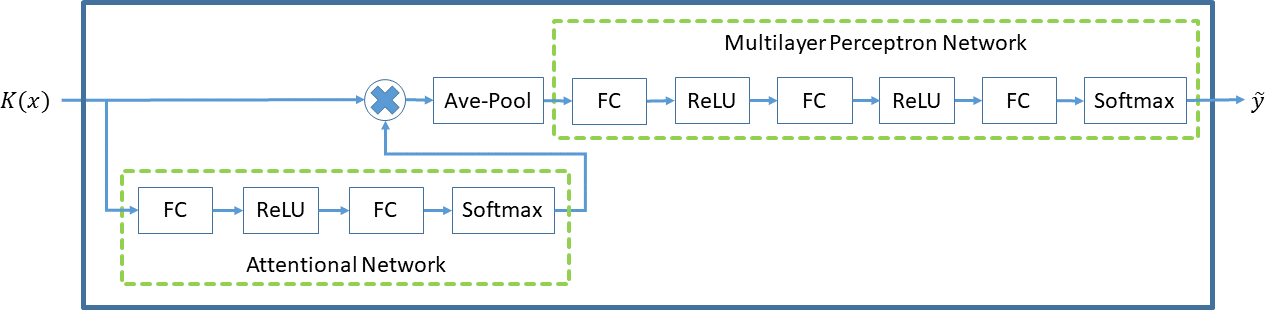
Now we would like to parameterize the functions $h,g$ in Eq. 9 using DNNs. Fig. 1 illustrates the architecture of our LMKL-Net, where “FC” denotes a fully connected layer, “ReLU” denotes rectified linear units nair2010rectified as the activation function, “Ave-Pool” denotes the average pooling operation over the kernels, and “Softmax” denotes a softmax function to normalize the inputs. Accordingly the parameter $\omega$ in $h$ is determined by the two FC layers in the attentional network (AN), and the parameter $\pi$ in $g$ is determined by the three FC layers in the multilayer perceptron network (MLP), respectively. By sequentially applying AN, average pooling, and MLP we indeed compute the decision function in Eq. 9. Empirically we find that ReLU leads to better performance with faster convergence than other activation functions, and adding more “ReLU$\rightarrow$FC” layers into the architecture, however, does not increase accuracy necessarily or significantly, but leads to more computational burden.

We train the network using ADAM kingma2014adam , a variant of SGD with adaptive learning rates, with mini-batches to learn both kernel weights and classifier parameters simultaneously, in contrast to the conventional MKL algorithms such as wrapper methods. LMKL-Net can achieve weak convergence in probability based on the analysis in bottou2016optimization for nonconvex optimization using SGD. Generally speaking, the computational complexity of LMKL-Net is linear to the number of its parameters, the size of mini-batches, and the number of iterations.

Figure 2: An equivalent architecture for accelerating training and inference of LMKL-Net by sharing weights.

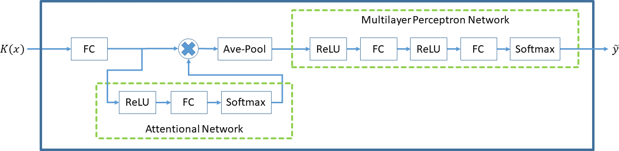
Training & Inference Acceleration: In large-scale problems where the training samples are dominant, most of the computation for optimizing LMKL-Net in Fig. 1 are spent on the two FC layers in AN and the first FC layer in MLP. To accelerate both training and inference, we enforce that the first FC layers in both AN and MLP share the same weights. This transfers Fig. 1 to a new network architecture as illustrated in Fig. 2. Empirically we observe almost identical accuracy on different datasets using both architectures, while the new architecture is trained significantly faster. Therefore in our experiments we report our performance based on the architecture in Fig. 2.

Discussion: The idea of neural network based LMKL solver can be utilized for solving some other MKL learning problems. For instance, in order to solve SimpleMKL in Eq. 6 we can feed a constant vector into AN to learn $\boldsymbol{\beta}$ and use an FC layer with non-negative weights as a constraint instead of MLP to learn $\boldsymbol{\alpha}$. We observe that in terms of accuracy in practice this network is always worse than LMKL-Net. Sparse learning in kernel SVMs are useful in practice to reduce the size of kernel matrix per data. To mimic this nice property, we can add the group sparsity into the learning of the first FC layer in Fig. 2. However, the investigation on these specific network design choices is out of scope of this paper, and we will consider them in our future work.

4 Experiments

Implementation: In our experiments, we utilize the cross entropy loss because it performs superiorly than other losses and can handle multiclass classification problems inherently. We set the output dimension in the first FC layer in Fig. 2 to 256D, and keep using it in MLP. The output dimension for the FC layer in AN is $N$ so that the entry-wise product operator can work. In our experiments using cross-validation we observe that higher dimensions than 256D do not necessarily lead to better accuracy but with remarkably longer running time, and the accuracy using lower dimensions starts to decrease. We initialize all FC layers randomly based on Gaussian distributions. We also observe that in our experiments having smaller weight decay krogh1992simple has little impact on the accuracy while larger weight decay worsens the performance significantly. Therefore we decide not to include weight decay in our experiments. We train the network for 200 epochs with batch size 256 and learning rate 0.001 for ADAM optimizer in DNN training. All these numbers are determined by cross-validation. We also utilize batch-normalization to accelerate the training. The results are reported based on 3 runs.

Benchmarks: For binary problems we test on 6 datasets, i.e. adult-8, news20, phishing, rcv1, real-sim, and w7a. For multiclass problems we test on 8 datasets, i.e. aloi, covtype, letter, protein, sensit (combined), sensorless, shuttle, and SVHN. We download all the datasets (scaled versions if available) from https://www.csie.ntu.edu.tw/~cjlin/libsvmtools/datasets/ which also lists the statistical information of the datasets such as numbers of training/validation/test data, classes and dimension of features. Please refer to the website for more dataset details.

Considering the memory limit we intentionally control the number of data samples for generating kernels. Specifically in each dataset we randomly select 20K samples from training/validation data if the samples are more than 20K, otherwise we use all of them. Similarly for test data, we randomly select 10K samples if there are more, otherwise use all. Then by referring to VGG MKL dataset at http://www.robots.ox.ac.uk/~vgg/software/MKL/ which consists of 10 Gaussian RBF kernels, we create 10 RBF kernels as well using the selected samples. We determine the window sizes in RBF-kernels to be proportional to the maximum Euclidean distance among the training features from 0.1 to 1 step by 0.1. We precompute all the kernels as the inputs for all the solvers.

To measure the classification performance, we utilize accuracy that is defined as the number of correctly classified samples divided by the total number of testing samples. The training and testing data samples have been balanced roughly.

Competitors: We compare LMKL-Net with some state-of-the-art MKL solvers with public code that can directly take kernels as input. We tune each solver so that we can report the best performance that we can achieve.

For binary classification, we test GMKL varma2009more , SMO-MKL Vishy10 , SPG-GMKL Jain12 , LMKL gonen08icml , Lp-MKL kloft2011lp , UFO-MKL orabona2011ultra , OBSCURE orabona2010online , and UNIFORM UNIFORM (i.e. average kernels with SVMs). We observe that GMKL, SMO-MKL, and SPG-GMKL always return identical results with different running speed, and thus report their results under the name of SPG-GMKL since it is fastest. Similarly for the two online learning methods, in our experiments OBSCURE outperforms UFO-MKL significantly in terms of both accuracy and running speed. Therefore, we only report the results of OBSCURE. We also observe that too much effort is needed such as heavily tuning parameters to make Lp-MKL work on our data and the results are often worse than others. For multiclass classification, we compare LMKL-Net with OBSCURE and UNIFORM because we find that most of existing code that we use cannot handle multiclass classification properly.

Note that among all the competitors OBSCURE is the most related to our LMKL-Net in terms of linear complexity in learning as well as its classification performance. OBSCURE utilizes group sparsity on classifier parameters (i.e. $\|\mathbf{w}\|_{2,p},1<p\leq 2$) as regularization and proposes a two-stage online learning algorithm (first online then batch) to optimize the primal formulation with complicate calculation. In contrast, LMKL-Net is a network based solver that can be efficiently trained using SGD. This remarkable difference in optimization leads to the fact that empirically LMKL-Net can be trained significantly faster with much smaller memory demand.

	adult-8	news20	phishing	rcv1	real-sim	w7a	average
UNIFORM	81.94	93.33	46.16	96.37	96.56	90.37	84.12
SPG-GMKL	84.13	90.27	95.26	95.57	92.21	97.05	92.42
LMKL	78.09	95.52	52.04	96.76	97.09	97.75	86.21
Lp-MKL	76.33	-	-	-	-	97.05	-
OBSCURE	84.22$\pm$0.09	94.68$\pm$0.03	97.25$\pm$0.00	96.55$\pm$0.05	96.94$\pm$0.00	98.50$\pm$0.02	94.69
Ours	84.62$\pm$0.15	93.53$\pm$0.03	98.17$\pm$0.25	96.71$\pm$0.07	96.42$\pm$0.09	98.74$\pm$0.03	94.70

Table 1: Comparison on binary classification accuracy ($\%$). “-” indicates that we cannot achieve reasonable performance on the dataset.

Figure 3: Illustration of training and testing (Top) loss and (Bottom) accuracy over epochs on different datasets.

4.1 Binary Classification

We first summarize our comparison results in Table 1. Overall our LMKL-Net outperforms all the other competitors, achieving the best in 3 out of 6 classes, while the other 3 best accuracies is obtained by LMKL. Compared with LMKL, however, LMKL-Net achieves 8.49% improvement on average in terms of accuracy. OBSCURE performs very closely to LMKL-Net.

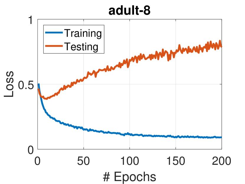
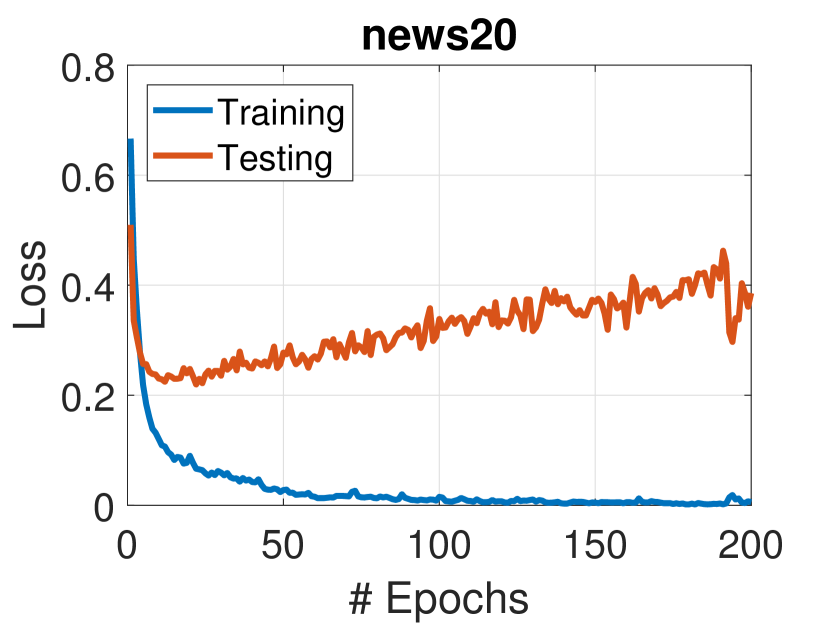
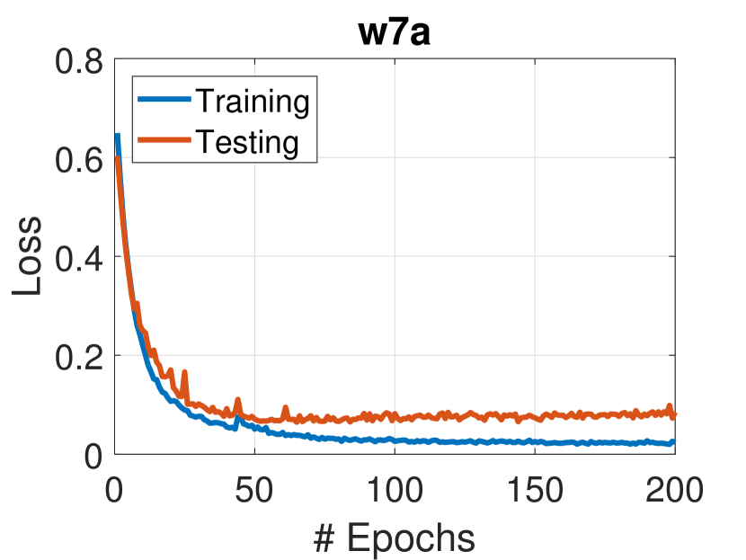
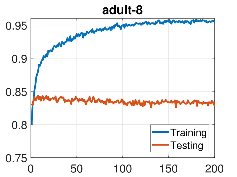
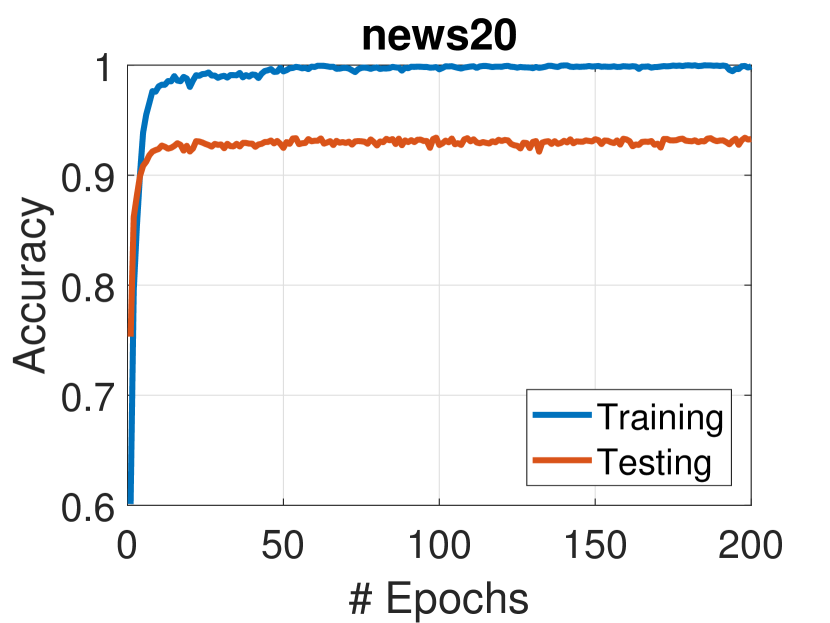
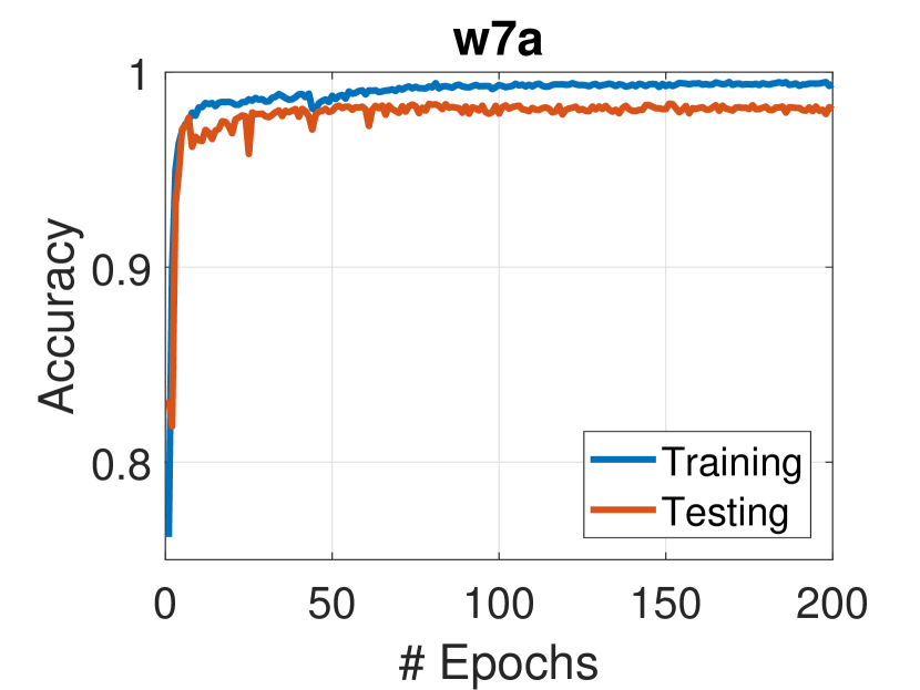
In order to understand LMKL-Net, we illustrate the loss and accuracy on training and test data in Fig. 3. We take for example adult-8, news20, and w7a. From the perspective of loss, we can observe clear overfitting in training on the first two datasets, as the testing loss increases with more epochs while the training loss decreases continuously. Surprisingly, we also observe that the quick and serious overfitting on adult-8 actually leads to very slow decrease in test accuracy, while on news20 such behavior is even hardly noticeable. This may explain why our solver performs worst on adult-8 among all the datasets. On the other hand, these observations also indicate the robustness of LMKL-Net in training and inference. In contrast, on w7a LMKL-Net is trained well, leading to the best performance among all the datasets.

We illustrate the kernel weights learned by LMKL-Net in Fig. 4 as well. To do so, we first marginalize $h(\mathbf{K}(z);\omega)$ in Eq. 10 for each sample $z$ over the training samples $x_{i},\forall i$ to compute an $M$-dim vector, and then compute the mean vectors over positive and negative samples in each test dataset, respectively. As we expect from the nature of data dependency, the patterns on each dataset are quite distinct. For instance, on news20 positives prefer the last four kernels while negatives prefer the rest. The variance in kernel weights is relatively small compared with the mean. Therefore for clarification we only show the mean values.

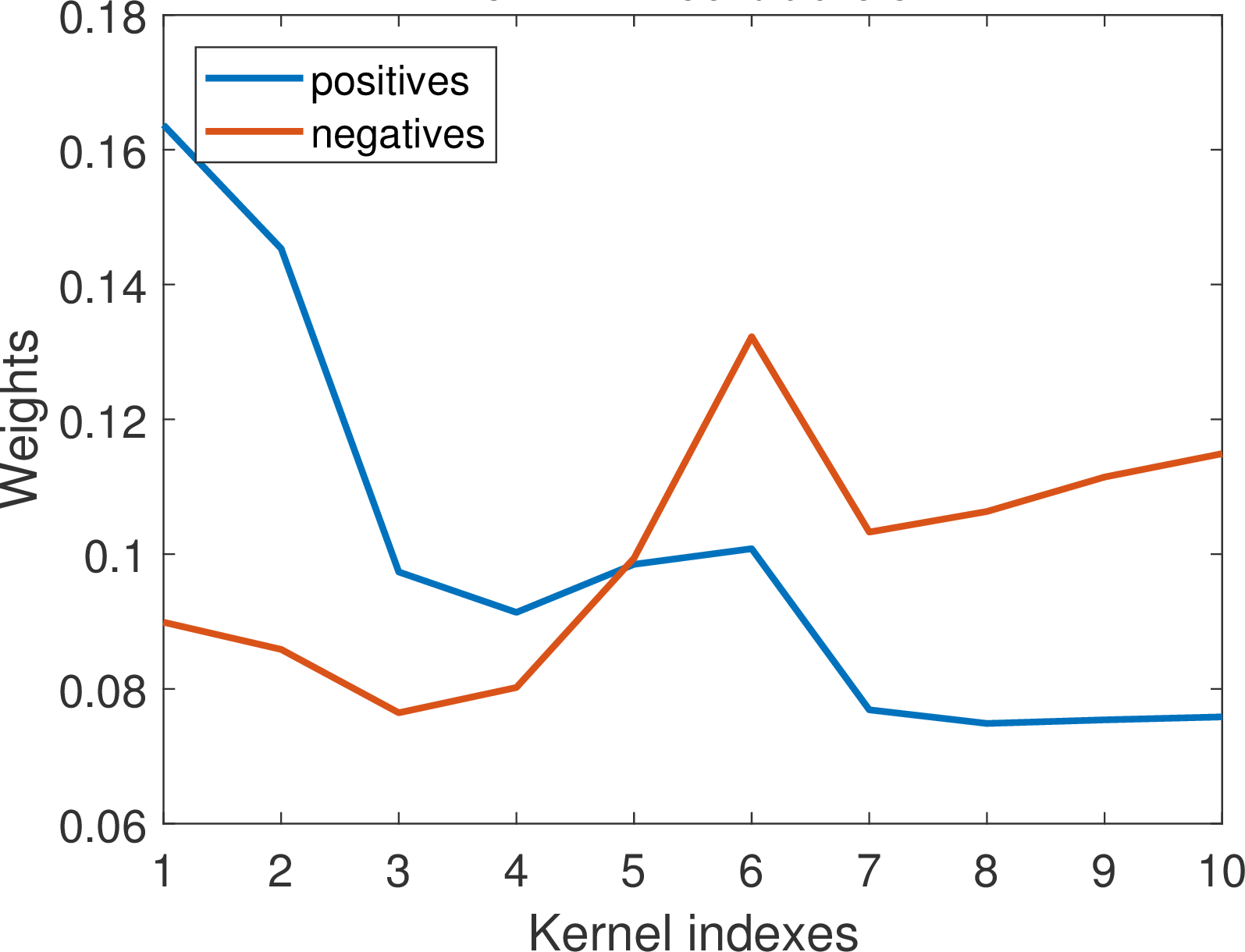
(a) adult-8

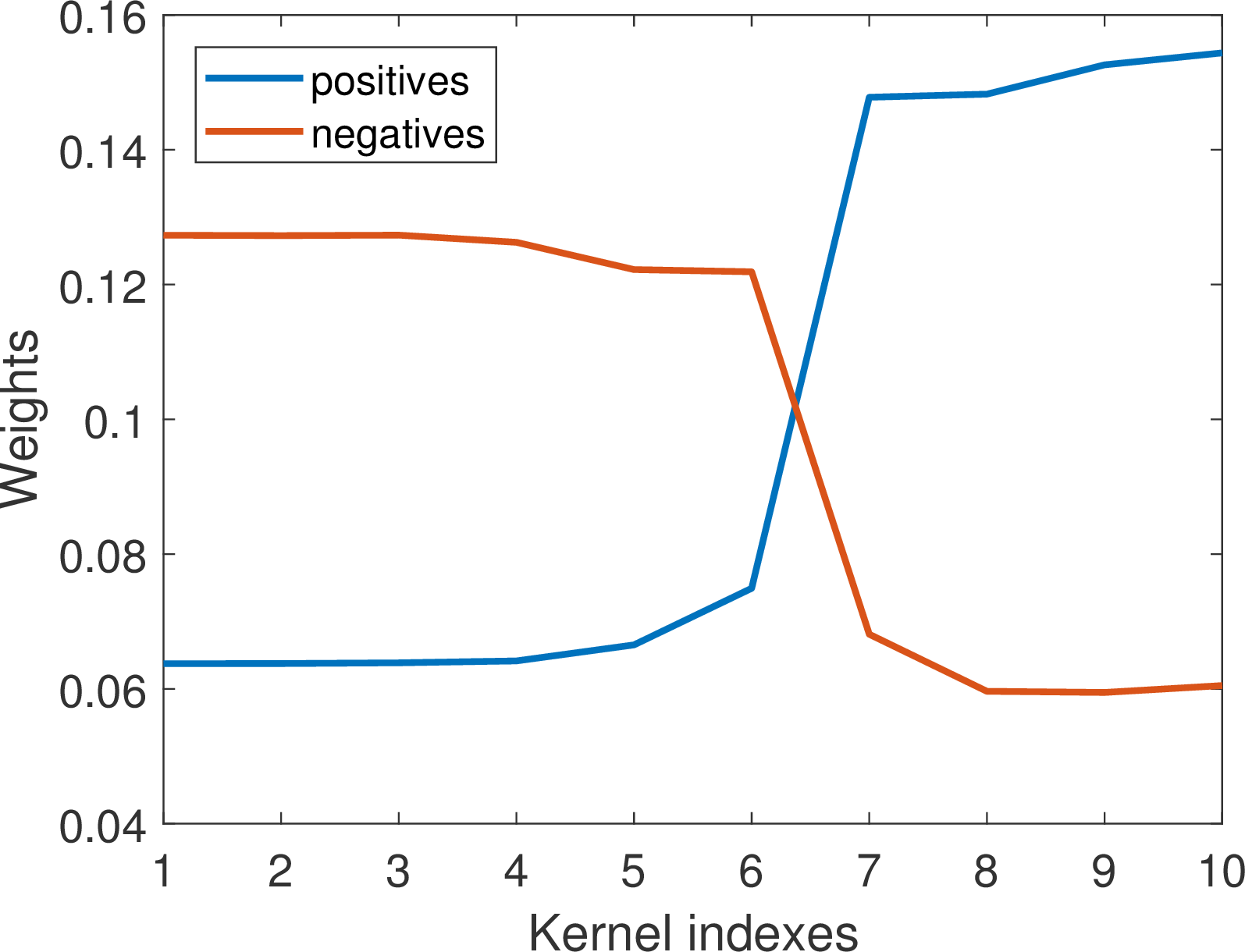
(b) news20

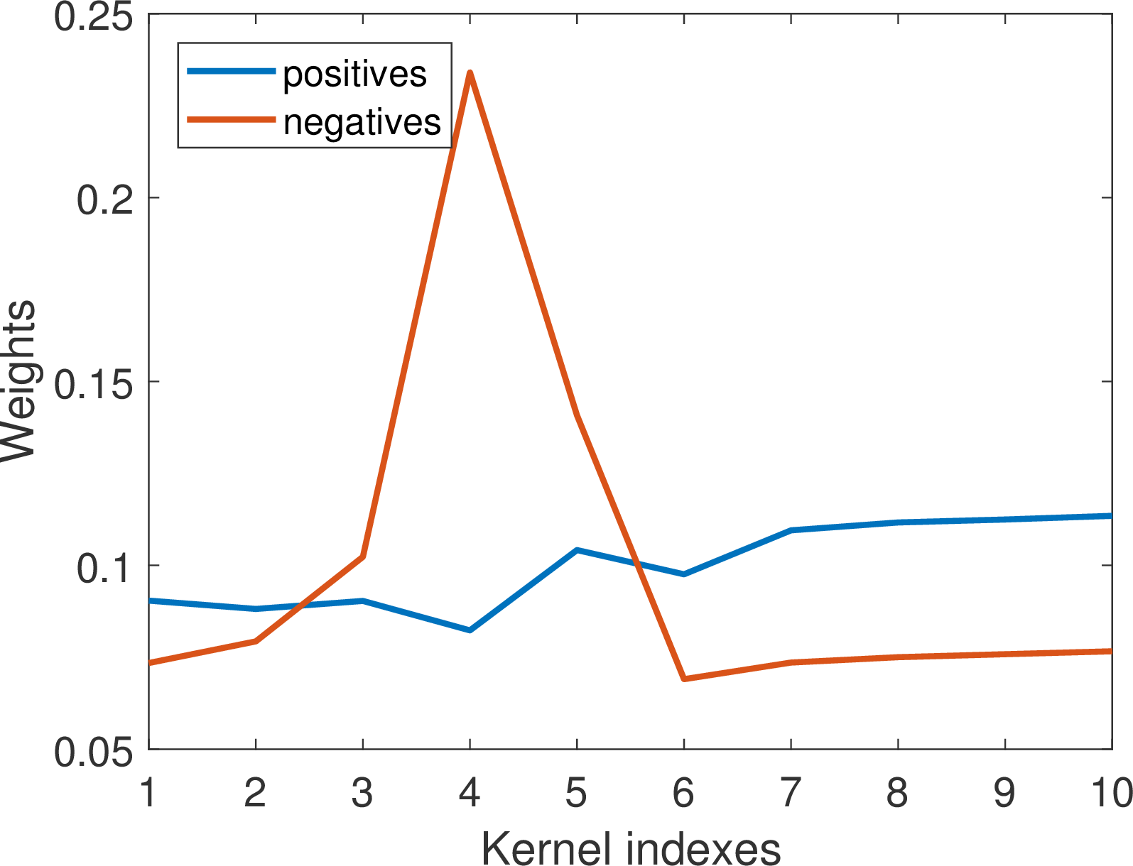
(c) w7a

Figure 4: Illustration of learned mean kernel weights by averaging over the test data in each binary dataset.

4.2 Multiclass Classification

Figure 5: Illustration of (top) loss and (bottom) accuracy in multiclass classification.

	UNIFORM	OBSCURE	Ours
aloi	86.74	89.60$\pm$0.14	89.37$\pm$0.16
covtype	82.12	83.56$\pm$0.07	82.48$\pm$0.09
letter	97.68	97.70$\pm$0.02	98.35$\pm$0.06
protein	70.24	69.95$\pm$0.11	69.92$\pm$0.27
sensit	85.20	83.76$\pm$0.05	84.93$\pm$0.15
sensorless	98.77	99.23$\pm$0.02	99.68$\pm$0.06
shuttle	99.19	99.84$\pm$0.01	99.87$\pm$0.01
SVHN	59.73	55.73$\pm$0.10	63.62$\pm$0.28
average	84.96	84.92	86.03

Table 2: Comparison on multiclass classification ($\%$).

We summarize the comparison results in Table 2. Again LMKL-Net performs the best overall with 1.11% improvement over OBSCURE.

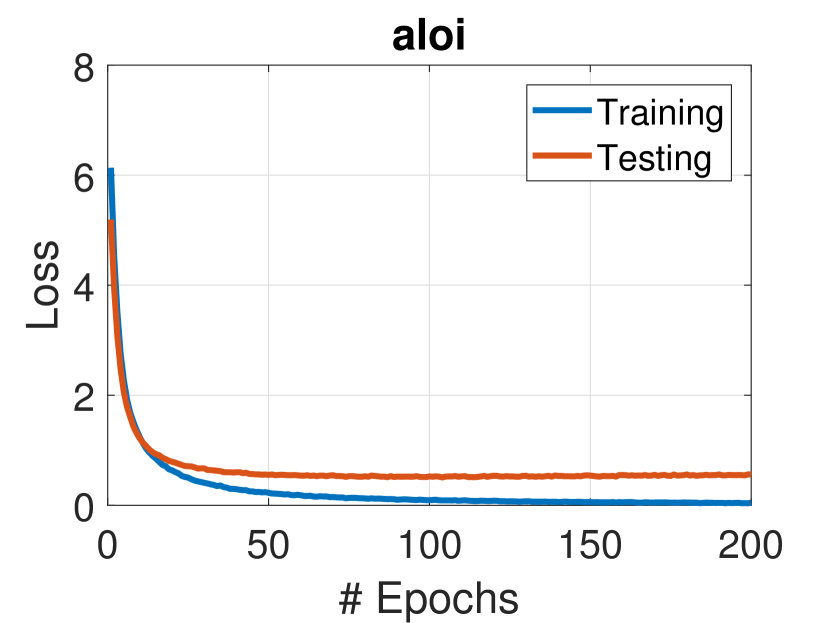
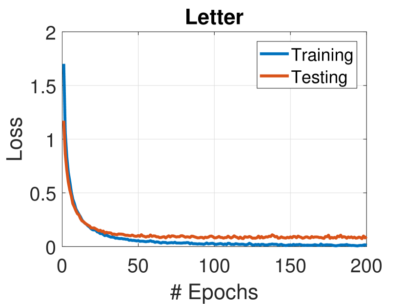
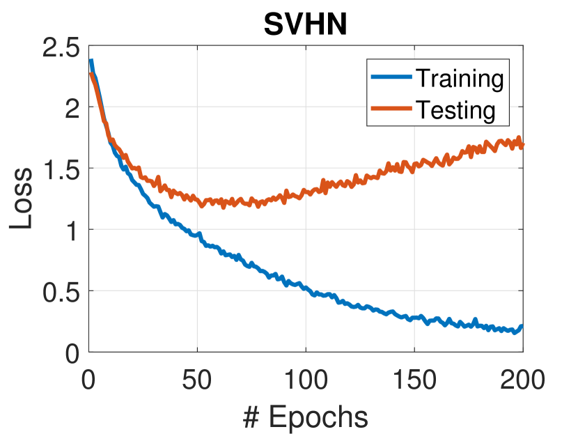
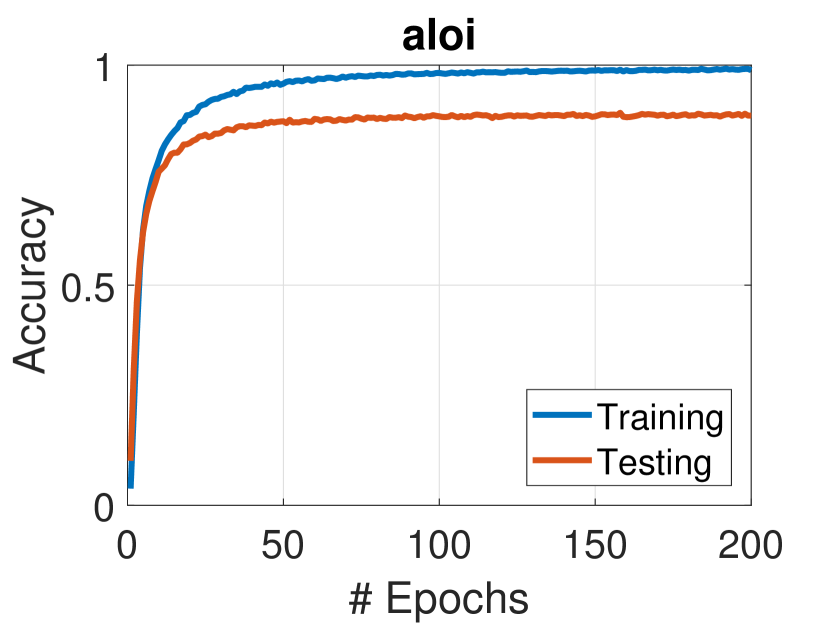
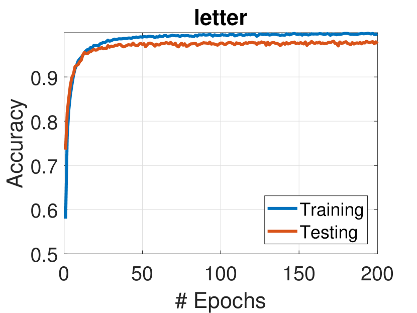
We also illustrate the training and testing behavior of our solver in Fig. 5. The observations here on loss and accuracy are quite similar to those in binary classification. Moreover it seems that the gaps between the training and testing curves for both loss and accuracy are consistent with each other. Namely, it is very likely that smaller gaps in loss will result in better training and testing accuracy, and vice versa.

We also test LMKL-Net on VGG MKL dataset as an example of using small-scale datasets. This dataset is created based on Caltech-101 where there are 101 object classes plus a background class. In our experiments we utilize the setup where for each class 15 images are sampled as training data and another 15 images as test data. 10 kernels are created as input. On this dataset our solver achieves $75.2\%$ with 0.6% improvement over the best number shown on the web page.

4.3 Memory Footprint & Computational Time

Typically it needs about 20GB hard disk to store the precomputed kernels per dataset. Due to the batch size of 256, we need about $256*20/20000=0.26$GB memory to store the data for SGD training. Compared with the memory for loading all the precomputed kernels, the ratio will be, roughly speaking, $0.26/20={\bf 0.013}$. Empirically Since we observe that even we project the input kernels to a lower dimensional space than 256D, our solver can still achieve similar performance. This indicates that the active memory or ratio can be much smaller dependent on the network architectures.

For computational time we take aloi dataset consisting of 1K classes as an example for large-scale learning. Our test machine has a GTX 1080 graphics card (GPU) and an i7-6850K@3.6GHz CPU. It takes more than 10 hours to learn OBSCURE with multi-threads on CPU. Our LMKL-Net is trained on GPU, and both need about 6s to traverse the dataset once (i.e. one epoch with about 20K samples). As we show in Fig. 3 and Fig. 5, our solver usually can converge empirically within 50 epochs. Based on these statistics, we can roughly compute the running time ratio as $6*50/(3600*10)={\bf 0.0083}$. On the other datasets we do observe that the training time of OBSCURE seems scalable with the number of classes given similar sizes of training data. For instance OBSCURE needs less than 5 minutes to be trained for binary classification (but still the fastest among the other solvers). In contrast, LMKL-Net has similar training speed across different datasets as long as the sizes of training data are roughly the same.

5 Conclusion

In this paper we propose a deep neural network, LMKL-Net, as an efficient solver for localized multiple kernel learning (LMKL) problems. LMKL-Net consists of two major components, i.e. an attentional network (AN) for learning the gating function and a multilayer perceptron (MLP) for learning a multiclass classifier in LMKL. We expect that the network can approximate the optimal functions in terms of accuracy given the input kernels. Empirically we demonstrate the performance of LMKL-Net on several benchmark datasets and compare it with some state-of-the-art MKL solvers. Overall LMKL-Net outperforms its competitors for both binary and multiclass classification. The robustness in training speed and the characteristic of SGD differentiate LMKL-Net from the other solvers, leading to about two orders of magnitude faster with much smaller memory footprint for large-scale learning.

References

- [1] M. Alioscha-Perez, M. Oveneke, D. Jiang, and H. Sahli. Multiple kernel learning via multi-epochs svrg. In 9th NIPS Workshop on Optimization for Machine Learning, 12 2016.
- [2] F. R. Bach. Exploring large feature spaces with hierarchical multiple kernel learning. In NIPS, pages 105–112, 2009.
- [3] F. R. Bach, G. R. Lanckriet, and M. I. Jordan. Multiple kernel learning, conic duality, and the smo algorithm. In ICML, page 6, 2004.
- [4] B. Bohn, M. Griebel, and C. Rieger. A representer theorem for deep kernel learning. CoRR, abs/1709.10441, 2017.
- [5] L. Bottou, F. E. Curtis, and J. Nocedal. Optimization methods for large-scale machine learning. arXiv preprint arXiv:1606.04838, 2016.
- [6] S. S. Bucak, R. Jin, and A. K. Jain. Multiple kernel learning for visual object recognition: A review. TPAMI, 36(7):1354–1369, 2014.
- [7] C. Cortes, M. Mohri, and A. Rostamizadeh. Learning non-linear combinations of kernels. In NIPS, pages 396–404, 2009.
- [8] M. Everingham, L. Van Gool, C. K. I. Williams, J. Winn, and A. Zisserman. The PASCAL Visual Object Classes Challenge 2009 (VOC2009) Results. http://www.pascal-network.org/challenges/VOC/voc2009/workshop/index.html.
- [9] P. Gehler and S. Nowozin. On feature combination for multiclass object classification. In ICCV, pages 221–228, 2009.
- [10] M. Gönen and E. Alpaydın. Localized multiple kernel learning. In ICML, 2008.
- [11] M. Gönen and E. Alpaydın. Multiple kernel learning algorithms. JMLR, 12(Jul):2211–2268, 2011.
- [12] M. Gönen, M. Kandemir, and S. Kaski. Multitask learning using regularized multiple kernel learning. In Neural Information Processing, pages 500–509, 2011.
- [13] Y. Han and G. Liu. Probability-confidence-kernel-based localized multiple kernel learning with {} norm. IEEE Transactions on Systems, Man, and Cybernetics, Part B (Cybernetics), 42(3):827–837, 2012.
- [14] S. N. Jagarlapudi, G. Dinesh, S. Raman, C. Bhattacharyya, A. Ben-Tal, and R. Kr. On the algorithmics and applications of a mixed-norm based kernel learning formulation. In NIPS, pages 844–852, 2009.
- [15] A. Jain, S. V. N. Vishwanathan, and M. Varma. Spg-gmkl: Generalized multiple kernel learning with a million kernels. In SIGKDD, August 2012.
- [16] P. Jawanpuria and J. S. Nath. Multi-task multiple kernel learning. In ICDM, pages 828–838, 2011.
- [17] P. Jawanpuria, J. S. Nath, and G. Ramakrishnan. Generalized hierarchical kernel learning. JMLR, 16(1):617–652, 2015.
- [18] S. Ji, L. Sun, R. Jin, and J. Ye. Multi-label multiple kernel learning. In NIPS, pages 777–784, 2009.
- [19] D. P. Kingma and J. Ba. Adam: A method for stochastic optimization. arXiv preprint arXiv:1412.6980, 2014.
- [20] M. Kloft, U. Brefeld, S. Sonnenburg, and A. Zien. Lp-norm multiple kernel learning. JMLR, 12(Mar):953–997, 2011.
- [21] A. Krogh and J. A. Hertz. A simple weight decay can improve generalization. In NIPS, pages 950–957, 1992.
- [22] Y. Lei, A. Binder, U. Dogan, and M. Kloft. Localized multiple kernel learning—a convex approach. In ACML, pages 81–96, 2016.
- [23] X. Li, B. Gu, S. Ao, H. Wang, and C. X. Ling. Triply stochastic gradients on multiple kernel learning. In UAI, 2017.
- [24] X. Liu, L. Wang, J. Zhang, and J. Yin. Sample-adaptive multiple kernel learning. In AAAI, pages 1975–1981, 2014.
- [25] Z. Long, Y. Lu, X. Ma, and B. Dong. Pde-net: Learning pdes from data. arXiv preprint arXiv:1710.09668, 2017.
- [26] A. F. T. Martins, N. Smith, E. Xing, P. Aguiar, and M. Figueiredo. Online learning of structured predictors with multiple kernels. In AISTATS, pages 507–515, 2011.
- [27] E. Meirom and P. Kisilev. Nuc-mkl: A convex approach to non linear multiple kernel learning. In AISTATS, pages 610–619, 2016.
- [28] H. N. Mhaskar and T. Poggio. Deep vs. shallow networks: An approximation theory perspective. Analysis and Applications, 14(06):829–848, 2016.
- [29] J. Moeller, P. Raman, S. Venkatasubramanian, and A. Saha. A geometric algorithm for scalable multiple kernel learning. In AIStats, pages 633–642, 2014.
- [30] J. Moeller, S. Swaminathan, and S. Venkatasubramanian. A unified view of localized kernel learning. In ICDM, pages 252–260, 2016.
- [31] Y. Mu and B. Zhou. Non-uniform multiple kernel learning with cluster-based gating functions. Neurocomputing, 74(7):1095–1101, 2011.
- [32] K. Murugesan and J. Carbonell. Multi-task multiple kernel relationship learning. In ICDM, pages 687–695, 2017.
- [33] V. Nair and G. E. Hinton. Rectified linear units improve restricted boltzmann machines. In ICML, pages 807–814, 2010.
- [34] K. Nguyen. Nonparametric online machine learning with kernels. In IJCAI, pages 5197–5198, 2017.
- [35] F. Orabona, L. Jie, and B. Caputo. Online-batch strongly convex multi kernel learning. In CVPR, pages 787–794, 2010.
- [36] F. Orabona, L. Jie, and B. Caputo. Multi kernel learning with online-batch optimization. JMLR, 13(Feb):227–253, 2012.
- [37] F. Orabona and J. Luo. Ultra-fast optimization algorithm for sparse multi kernel learning. In ICML, 2011.
- [38] P. Pavlidis, J. Weston, J. Cai, and W. N. Grundy. Gene functional classification from heterogeneous data. In Proceedings of the fifth annual international conference on Computational biology, pages 249–255, 2001.
- [39] A. Rakotomamonjy, F. R. Bach, S. Canu, and Y. Grandvalet. Simplemkl. JMLR, 9(Nov):2491–2521, 2008.
- [40] J. Sirignano and K. Spiliopoulos. Dgm: A deep learning algorithm for solving partial differential equations. arXiv preprint arXiv:1708.07469, 2017.
- [41] H. Song, J. J. Thiagarajan, P. Sattigeri, and A. Spanias. Optimizing kernel machines using deep learning. arXiv preprint arXiv:1711.05374, 2017.
- [42] S. Sonnenburg, G. Rätsch, C. Schäfer, and B. Schölkopf. Large scale multiple kernel learning. JMLR, 7(Jul):1531–1565, 2006.
- [43] E. V. Strobl and S. Visweswaran. Deep multiple kernel learning. In ICMLA, volume 1, pages 414–417, 2013.
- [44] L. Tang, J. Chen, and J. Ye. On multiple kernel learning with multiple labels. In IJCAI, pages 1255–1260, 2009.
- [45] M. Varma and B. R. Babu. More generality in efficient multiple kernel learning. In ICML, pages 1065–1072, 2009.
- [46] A. Vedaldi, V. Gulshan, M. Varma, and A. Zisserman. Multiple kernels for object detection. In ICCV, pages 606–613, 2009.
- [47] S. V. N. Vishwanathan, Z. Sun, N. Theera-Ampornpunt, and M. Varma. Multiple kernel learning and the SMO algorithm. In NIPS, December 2010.
- [48] E. Weinan, J. Han, and A. Jentzen. Deep learning-based numerical methods for high-dimensional parabolic partial differential equations and backward stochastic differential equations. Communications in Mathematics and Statistics, 5(4):349–380, 2017.
- [49] J. Yang, Y. Li, Y. Tian, L. Duan, and W. Gao. Group-sensitive multiple kernel learning for object categorization. In ICCV, pages 436–443, 2009.
- [50] A. Zien and C. S. Ong. Multiclass multiple kernel learning. In ICML, pages 1191–1198, 2007.