Many-Body Dissipative Flow of a Confined Scalar
Bose-Einstein Condensate Driven by a Gaussian Impurity

Abstract

The many-body dissipative flow induced by a mobile Gaussian impurity harmonically oscillating within a cigar-shaped Bose-Einstein condensate is investigated. For very small and large driving frequencies the superfluid phase is preserved. Dissipation is identified, for intermediate driving frequencies, by the non-zero value of the drag force whose abrupt increase signals the spontaneous downstream emission of an array of gray solitons. After each emission event, typically each of the solitary waves formed decays and splits into two daughter gray solitary waves that are found to be robust propagating in the bosonic background for large evolution times. In particular, a smooth transition towards dissipation is observed, with the critical velocity for solitary wave formation depending on both the characteristics of the obstacle, namely its driving frequency and width as well as on the interaction strength. The variance of a sample of single-shot simulations indicates the fragmented nature of the system; here it is found to increase during evolution for driving frequencies where the coherent structure formation becomes significant. Finally, we demonstrate that for fairly large particle numbers in-situ single-shot images directly capture the gray soliton’s decay and splitting.

I Introduction

Dark solitons are fundamental nonlinear excitations that are found to spontaneously emerge in diverse physical systems ranging form nonlinear optics zakharov ; drummond ; yuridavies to repulsively interacting one-dimensional (1D) Bose-Einstein condensates (BECs) pethick ; stringari ; djf ; siambook and from water waves chabchoub to magnetic materials colostate . In the BEC setting, there exist numerous distinct mechanisms of spontaneous generation of these solitonic structures that have been theoretically proposed and also experimentally implemented. These density depleted states can be formed by e.g. imprinting a phase distribution (or a density one, or both) in the BEC burger ; Denschlag ; becker , in interference experiments, e.g. during the collision of two condensates weller ; theo ; Reinhardt ; Scott , or by perturbing the BEC with localized impurities moving relative to the condensate dutton ; Engels_2007 .

In this latter context dark soliton generation induced by the motion of an impurity through the BEC has been intensely studied Hakim ; Leboeuf ; Pavloff ; Brazhnyi ; Radouani ; Carretero ; Hans ; Syafwan , and it can be connected with the onset of dissipation Frisch ; Winiecki ; Astra . Landau’s criterion sets the bound below which the flow remains dissipationless and no excitations are present in the system Landau . This bound for dilute BECs is the Bogoliubov speed of sound. However, numerous of the aforementioned theoretical and experimental studies have tested this criterion and estimations of significantly smaller critical velocities have been reported Ketterle_1999 ; Ketterle_2000 ; Engels_2007 , being attributed to the confinement geometry and/or finite temperature effects.

In the above investigations impurities of different shape and width have been considered, showcasing that above an obstacle dependent critical velocity gray solitons, i.e. moving dark solitons, and sound waves (see e.g. Refs. Radouani ; Engels_2007 and references therein) may be generated. In fact, under suitable conditions, more complicated dispersive shock wave patterns may also be formed Hakim ; Kamchatnov (see also here Refs. El1 ; El2 ; Hoefer for higher dimensional settings and hoefer2 for a recent review of the latter theme of research). This structure formation occurs whenever the velocity of the obstacle becomes locally larger than the (local) speed of sound Carretero ; Frisch ; Winiecki ; Huepe , and ceases to exist for high speed impurities Radouani ; Engels_2007 ; Pavloff . However, numerous questions still remain for which a many-body (MB) treatment of the problem has been suggested concerning e.g., the presence of dissipation even for very small obstacle velocities Astra , or the prediction of a smoother transition towards dissipation Ketterle_1999 . Additionally, in this latter context, the spontaneous generation of the so-called quantum dark solitons sachadark3 ; sachadark2 ; sachadark1 ; mishmash1 ; mishmash2 ; martin ; sacha ; sacha17 is still an open question. These quantum dark solitons are known to be fragmented entities, i.e. being more adequately described by more than a single particle state, especially so when instabilities –at the single particle state level– or time-dependent dynamical processes are involved Katsimiga ; lspp ; lgspp . Thus, yet another interesting prospect is to examine how the aforementioned spontaneous generation of these states is related to the onset of fragmentation.

Motivated by earlier experiments on this topic Ketterle_1999 ; Ketterle_2000 but also by the ongoing interest regarding the notion of dissipation in quantum fluids Wright ; Ryu ; Eckel ; Jendrezejewski ; Weimer ; Roati in the current effort we explore the breaking of superfluidity and the subsequent soliton generation upon considering in the MB framework the influence of an oscillating repulsive Gaussian impurity penetrating the bosonic cloud. The specific setup examined herein has been partially motivated by an earlier mean-field (MF) study where the controllable dark soliton creation was demonstrated planist . We provide direct numerical evidence of smaller critical velocities compared to the MF scenario for the onset of dissipation and the subsequent coherent structure formation. In particular, it is shown that this critical velocity depends on the trapping geometry, the characteristics of the impurity, and the interaction strength and thus the corresponding speed of sound Ketterle_2000 . It is found that the trap significantly lowers this critical value Fedichev , when compared to the untrapped scenario, a feature that may be expected on the basis of its variable density locally modifying the speed of sound. Moreover, wider obstacles and also effectively denser clouds result again in the significant decrease of this critical velocity. More importantly, we further verify earlier suggestions of a smoother transition towards dissipation Ketterle_1999 that naturally emerges herein when MB effects are taken into account.

To systematically study the MB driving dynamics Mistakidis_per ; Mistakidis_per1 of a Gaussian impurity penetrating a 1D harmonically confined bosonic cloud, we use the Multi-Configuration Time-Dependent Hartree Method for bosons (MCTDHB) cederbaum1 ; cederbaum2 and contrast our findings with MF theory. We investigate the system’s dynamical response covering the range from weak to strong driving frequencies. To infer about the dissipative flow we inspect the drag force Astra ; khamis ; Kato ; Pinsker exerted on the fluid by the Gaussian impurity. For very small or large driving frequencies the superfluid is dissipationless. We demonstrate that dissipation, occurring for intermediate driving frequencies, is followed by the spontaneous downstream emission, with respect to the impurity’s motion, of an array of moving gray solitary waves that naturally emerge in a MB environment and dispersive sound waves moving upstream. This important outcome reveals, further adding to the existing studies regarding the aforementioned solitary waves sachadark3 ; sachadark2 ; sachadark1 ; mishmash1 ; mishmash2 ; martin ; sacha ; sacha17 , that such nonlinear excitations can be dynamically excited in a MB system and are thus of fundamental origin. Each of these solitary waves soon after its formation is found to decay sachadark3 ; sachadark2 ; Katsimiga ; lspp and split into two daughter gray solitary waves that remain robust propagating in the BEC background for large evolution times. Additionally, utilizing single-shot simulations, the fragmented nature of the system is showcased probed by the evolution of the variance of a sample of single-shots. In particular, fragmentation is found to be maximal when dissipation occurs, a result that holds as such for a wide parametric window. Furthermore, we provide direct numerical evidence of the aforementioned gray solitons’ generation and more importantly their subsequent decay and splitting in the present type of a dynamical MB setting. We showcase the latter by simulating in-situ single shot images upon considering a fairly large bosonic cloud. Finally, we retrieve superfluidity for high speed impurities Paris namely for velocities being almost six times the bulk (i.e. the maximal value measured around the trap center) speed of sound.

The presentation of our work is structured as follows. In Section II the model setup and the MB ansatz are provided. Section III contains our numerical findings both in the single orbital MF case and in the MB correlated approach. In Section IV we offer experimentally testable evidence of the observed MB evolution by simulating single-shot images. Our results are summarized in Section V, along with interesting directions for future study. Finally, in Appendix A we discuss the convergence behavior of our numerical results.

II Driving Scheme and many-body ansatz

In the following we consider the MB quantum dynamics of a scalar harmonically confined 1D BEC being relaxed to its ground state, with a Gaussian impurity located initially ($t=0$) at the right edge of the cloud ($x>0$) where the density is almost vanishing, and subsequently crossing the BEC towards its left edge ($x<0$). Such a cigar-shaped geometry is experimentally realizable upon considering a strong confinement along the perpendicular $y,z-$directions, namely $\omega_{\perp}>>\omega_{x}\equiv\Omega$. To study the out-of-equilibrium dynamics of this system we consider the following form for the driving potential

$$V_{D}(x,t)=V_{ext}(x)+V_{G}(x,t).$$ (1)

In Eq. (1) the first term is the standard parabolic potential, $V_{ext}(x)=\left(1/2\right)m\Omega^{2}x^{2}$, of strength $\Omega$, while $m$ is the particle mass. The second part corresponds to the mobile Gaussian impurity $V_{G}(x,t)=\frac{A}{\sqrt{2\pi}w}\exp\left\{-\frac{[x-x_{D}(t)]^{2}}{2w^{2}}\right\}$. Such time-dependent localized potentials may stem from an intensely focused laser beam spot moving through the condensate Ketterle_1999 ; Ketterle_2000 . Here, $A>0$ is the amplitude of the Gaussian impurity corresponding to a repulsive potential for the atoms and $w$ is its width. Initially, the system is in its ground state for $x_{D}(t=0)=B$. The initial position of the obstacle, $B\approx R_{TF}$, is located at the right edge of the bosonic cloud possessing approximately a Thomas-Fermi profile of the form $\rho^{(1)}(x;0)\approx\sqrt{m\Omega^{2}\left(R^{2}_{TF}-x^{2}\right)/2g_{1D}}$. The Thomas-Fermi radius reads $R_{TF}=\sqrt{\frac{2\mu}{m\Omega^{2}}}$ (see Fig. 1), where $\mu$ is the chemical potential, while $g_{1D}$ is the effective interaction strength (see below). At $t=0$ the impurity commences an oscillatory motion $x_{D}(t)=B\cos(\omega_{D}t)$ with frequency $\omega_{D}=2\pi/T_{D}$, for either half ($0\leq t\leq t_{1}=T_{D}/2$) or one ($0\leq t\leq t_{1}=T_{D}$) oscillation period corresponding to a single or double crossing of the impurity through the BEC respectively. For $t>t_{1}$ the impurity remains stationary at $x_{D}(t)=B\cos(\omega_{D}t_{1})$ and the system is left to evolve in the absence of external driving. Note here that the velocity of the obstacle during $0\leq t\leq t_{1}$ reads $u_{D}=-B\omega_{D}\sin(\omega_{D}t)=\mp\omega_{D}\sqrt{B^{2}-x_{D}^{2}(t)}$. It then follows that the ratio of $u_{D}$ and the unperturbed local speed of sound at the position of the impurity is $c_{0}\big{(}x_{D}(t)\big{)}=\sqrt{gm^{-1}\rho^{(1)}\big{(}x_{D}(t);0\big{)}}$, and it is approximatively constant throughout the driving. Thus, we can relate the values of $\omega_{D}$ with the characteristic (and commonly employed) velocity ratio $u_{D}(x_{D})/c_{0}(x_{D})\equiv u_{D}/c_{0}\approx\sqrt{2}\omega_{D}/\Omega$, since $B\approx R_{TF}$.

The MB Hamiltonian consisting of $N$ bosons each with mass $m$ trapped in the 1D potential of Eq. (1) reads

$$\begin{split}H(x_{1},x_{2},...,x_{N};t)=&\sum_{i=1}^{N}\left[-\frac{\hbar^{2}}{2m}\partial_{x_{i}}^{2}+V_{D}\left(x_{i};t\right)\right]\\ &+g_{1D}\sum_{i<j}\delta(x_{i}-x_{j}).\\ \end{split}$$ (2)

Operating in the ultracold regime, the short-range delta interaction potential between particles located at positions $x_{i}$ can be adequately described by $s$-wave scattering. The effective interaction strength in this case is defined as $g_{1D}=\left(2\hbar^{2}a_{0}/ma^{2}_{\perp}\right)\left(1-\frac{|\zeta(1/2)|a_{0}}{\sqrt{2}a_{\perp}}\right)^{-1}$ g1d , where $a_{\perp}=\sqrt{\hbar/\left(m\omega_{\perp}\right)}$ is the transverse harmonic oscillator length characterized by $\omega_{\perp}$, and $a_{0}$ denotes the free space 3D $s$-wave scattering length. In the present investigation we consider the dynamics of repulsively interacting bosons namely $g_{1D}>0$. Experimentally $g_{1D}$ can be adjusted either via $a_{0}$ utilizing magnetic or optical Feshbach resonances Inouye ; Chin or through the corresponding $\omega_{\perp}$ utilizing confinement-induced resonances g1d . Our setup can be to a good approximation realized by considering e.g. a gas of ⁸⁷Rb atoms. To render the Hamiltonian of Eq. (2) dimensionless the following transformations are performed for the energy, length and time scales: $\tilde{H}=\left(\hbar\omega_{\perp}\right)^{-1}~{}H$, $\tilde{x}=\sqrt{\left(m\omega_{\perp}\right)/\hbar}~{}x$, and $\tilde{t}=\omega_{\perp}~{}t$. According to the above the interaction strength, Gaussian amplitude and width are expressed in dimensionless units of $\tilde{g}=\sqrt{m/\left(\hbar^{3}\omega_{\perp}\right)}~{}g_{1D}$, $\tilde{A}=\sqrt{m/\left(\hbar^{3}\omega_{\perp}\right)}~{}A$, and $\tilde{w}=\sqrt{\left(m\omega_{\perp}\right)/\hbar}~{}w$ respectively. For convenience henceforth we shall omit the tildes, and all the numerical values given are to be understood in the aforementioned dimensionless units. Furthermore, throughout this work the trapping frequency, $\Omega=0.1$, the Gaussian amplitude, $A=1/2$ and the width, $w=0.1$ (being always smaller than the corresponding healing length $\xi=1/\sqrt{2\mu}$), are held fixed unless it is stated otherwise. We remark here that larger values of either $A$ or $w$ lead to a decrease of the critical velocity and an enhanced number of emitted solitons Hakim . Therefore, we are left with two free parameters namely $g$ and $\omega_{D}$.

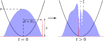
Figure 1: (Color online) Schematic representation of the driving dynamics, which leads to the spontaneous generation of two, in the sketch shown, downstream dark solitons. Notice that the width of the impurity (denoted by the thin red Gaussian curve) is much smaller than the corresponding healing length.

To systematically take into account the important particle correlations inherent to the system we utilize the MCTDHB approach cederbaum1 ; cederbaum2 , which is a reduction of the more general Multi-Layer-Multi-Configuration Hartree method for bosonic and fermionic Mixtures (ML-MCTDHX) Cao ; matakias ; moulosx . The MB wavefunction of the system $\Psi_{MB}(x_{1},\dots,x_{N};t)$, with ($x_{1},\dots,x_{N}$) labelling the spatial coordinates of the atoms, is constructed by permanents that are built upon $M$ distinct time-dependent single particle functions (SPFs)

$$\begin{split}&\Psi_{MB}(x_{1},\dots,x_{N};t)=\sum_{\begin{subarray}{c}n_{1},\dots,n_{M}\\ \sum n_{i}=N\end{subarray}}A_{(n_{1},\dots,n_{M})}(t)\times\\ &\sum_{i=1}^{N!}\mathcal{P}_{i}\left[\prod_{j=1}^{n_{1}}\varphi_{1}(x_{j};t)\cdots\prod_{j=1}^{n_{M}}\varphi_{M}(x_{K(M)+j};t)\right].\end{split}$$ (3)

In the above expression $\mathcal{P}$ is the permutation operator exchanging the particle positions $x_{i}$, $i=1,\dots,N$, $\varphi_{l}(x;t)$, $l=1,2,...,M$, denote each SPF, $K(M)\equiv\sum^{M-1}_{k=1}n_{k}$, and $A_{(n_{1},\dots,n_{M})}(t)$ correspond to the time-dependent expansion coefficients of a particular permanent. $N$ refers to the total particle number and $n_{k}$ is the occupation number of the $k$-th SPF. Following e.g. the McLachlan time-dependent variational principle McLachlan for the generalized ansatz of Eq. (3) yields the MCTDHB cederbaum1 ; cederbaum2 ; matakias ; moulosx equations of motion. These consist of a set of $\frac{(N+M-1)!}{N!(M-1)!}$ linear differential equations for the expansion coefficients and $M$ nonlinear integro-differential equations for the SPFs $\varphi_{i}(x;t)$.

The spectral representation of the one-body reduced density matrix reads

$$\rho^{(1)}(x,x^{\prime};t)=N\sum\limits_{i=1}^{M}{{n_{i}}(t){\phi_{i}}(x,t)}\phi_{i}^{*}(x^{\prime},t),$$ (4)

where $M$ refers to the number of natural orbitals, $\phi_{i}(x;t)$, used. The latter are the eigenfunctions of the one-body reduced density matrix Titulaer ; Naraschewski ; Sakmann being normalized to unity, while $n_{i}$ are the corresponding eigenvalues or natural populations. Note here that the one-body density $\rho^{(1)}(x;t)\equiv\rho^{(1)}(x,x^{\prime}=x;t)$, and for $M\rightarrow\infty$, $\rho^{(1)}(x;t)$ becomes the exact one-body density $\tilde{\rho}^{(1)}(x;t)$. Our MB wavefunction $\Psi_{MB}(x_{1},\dots,x_{N};t)$ reduces to the MF one, $\Psi_{MB}(x_{1},\dots,x_{N};t)\rightarrow\Psi_{MF}(x_{1},\dots,x_{N};t)$, when the corresponding natural occupations obey $n_{1}(t)=1$, $n_{i\neq 1}(t)=0$. In the latter case the first natural orbital $\phi_{1}(x;t)$ reduces to the MF wavefunction which for the $N$-particle system is $\Psi_{MF}(x_{1},\dots,x_{N};t)=\prod_{i=1}^{N}\phi_{1}(x_{i};t)$ and obeys the Gross-Pitaevskii equation stringari . Finally, we remark that the above-mentioned natural populations $n_{i}(t)\in[0,1]$ characterize the degree of the system’s fragmentation or interparticle correlations Penrose ; Mueller . For only one macroscopically occupied orbital the system is said to be condensed, otherwise it is fragmented.

III Non-Equilibrium Driven Quantum Dynamics

A direct comparison of the MF and the MB driven dynamics can be deduced by inspecting the spatio-temporal evolution of the one-body density, $\rho^{(1)}(x;t)$, shown in Figs. 2 $(a_{1})$-$(a_{3})$ and $(b_{1})$-$(b_{3})$ respectively. In all cases the obstacle is initially placed at $x\gtrsim R_{TF}$, the oscillation frequency is $\omega_{D}=0.05$, while $B=25$ ($B=12$) for $g=1$ (for $g=0.1$).

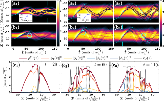
Figure 2: (Color online) $(a_{1})$-$(a_{2})$ [$(b_{1})$-$(b_{2})$] Evolution of the one-body density, $\rho^{(1)}(x;t)$, within the MF [MB] approach for a single crossing of the obstacle through the BEC. From left to right in each row the intraspecies interaction coefficient increases from $g=0.1$ to $g=1$. $(a_{3})$ [$(b_{3})$] Same as the above but for an oscillation period of the obstacle. In all cases dashed curves indicate the position of the Gaussian impurity and circles showcase the decay events observed in the MB scenario. Insets illustrate the phase profile, $\theta(x)$, for the MF case, at $t=120$ [see the vertical cyan lines in $(a_{1})$, $(a_{2})$] after all the solitons are generated. Notice that there is a series of jumps, none of which is exactly $\pi$ because none of the produced MF gray solitons is stationary. $(c_{1})$- $(c_{3})$ Profile snapshots of $\rho^{(1)}(x;t)$, as well as of the densities $\left|\phi_{i}(x,t)\right|^{2}$ with $i=1,\dots,4$, of the four natural orbitals used in the MB approach for $g=1$ for an oscillation period at different time instants of the evolution indicated by the solid cyan lines in $(b_{3})$. Arrows here, indicate the location of the gray solitons while dashed rectangles capture the formation of the domain-walls building between the higher-lying orbitals. The Gaussian impurity amplitude and width in these cases are magnified to provide better visibility. The initial ground state configuration contains $N=100$ bosons and the trapping frequency is fixed to $\Omega=0.1$. $B=25$ ($B=12$) for $g=1$ ($g=0.1$) so as to initialize the Gaussian of width $w=0.1$ and amplitude $A=0.5$ at the right edge of the TF cloud.

In both approaches, it is observed that from the very early stages of the out-of-equilibrium dynamics a density imbalance between the left and the right side of the impurity during its motion occurs. This density imbalance results in the spontaneous emission of both a downstream (behind the impurity) and an upstream (in front of the impurity) disturbance with respect to the obstacle’s motion. This emission is activated when the velocity of the impurity becomes greater than the local speed of sound ($c(x)=\sqrt{g\rho^{(1)}(x)}$). Note that despite placing the impurity at extremely low densities our used profile of the velocity ensures that at the beginning of the driving dynamics the impurity is subsonic, i.e. $u_{D}<c$. The disturbance behind the driver arises in the form of gray solitons, while the one in front of it consists of dispersive sound waves. In particular, three and four almost regularly spaced solitons are clearly emitted by the impurity for a single crossing (i.e., $t_{1}\in$ [0, $T_{D}/2$]), of the obstacle through the condensate in the MF case illustrated in Figs. 2 $(a_{1})$ and $(a_{2})$ for $g=0.1$ and $g=1$ respectively (see also Table 1). Each of the solitary waves formed develops a characteristic phase jump always smaller than $\pi$ as it is evident in the corresponding phase profiles, $\theta(x)$, depicted as insets in Figs. 2 $(a_{1})$ and $(a_{2})$ for $g=0.1$ and $g=1$ respectively at $t=120$. The number of solitary waves generated in both approaches is presented in Table 1 for different driving frequencies and upon increasing the interaction strength. Notice that in both approaches for fixed $\omega_{D}$ the number of coherent structures emitted by the source increases for increasing $g$. We remark here that among the excitations formed, we exclude all waves having a numerically identified speed $u_{sol}\gtrsim 0.95c$, since for these states we cannot assign a clear phase jump and thus cannot definitively distinguish them from sound waves.

In the corresponding MB dynamics the following key differences when compared to the MF scenario are discernible. The emission of solitary waves remains the same as in the MF approximation for small $g$ values but is slightly larger upon increasing $g$ with the solitons emitted being five in the MB approach instead of four in the MF case (see again here Table 1, for $\omega_{D}=0.05$ and $g=1$). Furthermore, and also independently of the magnitude of the interaction strength most of the solitons soon after their formation decay in the MB scenario sachadark3 ; sachadark2 ; sachadark1 ; sacha ; sacha17 ; lgspp ; lspp . This decay is followed by a splitting of each gray solitonic structure into two daughter solitary waves. Case examples of such decay and splitting events are indicated with solid circles in Figs. 2 $(b_{1})$-$(b_{3})$. These daughter states are more robust and propagate in the BEC background for large evolution times. The aforementioned process repeats itself when considering the dynamics for a full period of oscillation, with the spontaneous emission of downstream gray solitons and upstream dispersive sound waves taking place whenever the obstacle’s motion becomes locally supersonic, i.e. $u_{D}>c$ [see Figs. 2 $(a_{3})$, $(b_{3})$].

Solitary Wave Counting
$\omega_{D}$	0.02	$0.05$	$0.08$	$0.2$
MF $g$=1.0	$0$	4	5	0
MB $g$=1.0	0	5	6	0
MF $g$=0.1	0	3	2	0
MB $g$=0.1	0	3	2	0

Table 1: Solitary wave counting for a single crossing of the impurity through the BEC, upon increasing both the driving frequency and the interparticle interaction strength. Note that among the excitations formed we exclude all waves having a numerically identified speed $u_{sol}\gtrsim 0.95c$. For such high speeds no clear phase jump can be attributed to these structures as can be deduced by inspecting the insets in Figs. 2 $(a_{1})$ and $(a_{2})$.

To gain further insight into the generation of gray solitons within the MB approach in Figs. 2 $(c_{1})$-$(c_{3})$ profile snapshots of the one-body density as well as for the four natural orbitals used are presented for initial, intermediate, and longer evolution times for $g=1$. In the one-body density presented in all Figs. 2 $(c_{1})$-$(c_{3})$, some of the density dips correspond to solitary wave structures associated predominantly with the first orbital. See e.g. the gray soliton generated in $\rho^{(1)}(x;t=28)$ indicated by a black arrow in Fig. 2 $(c_{1})$, that is clearly supported by a density dip developed in the first orbital. Others, especially so at later times, and most notably so at $t=110$ depicted in Fig. 2 $(c_{3})$ may be associated with higher orbitals such as the second one (see again black arrows here). However, a key observation emerging from the breakdown of the one-body density through the orbitals is that not all substantial density dips in the MB case are associated with gray solitons, contrary to what would be the case in the MF scenario. Instead, numerous ones among them, notably at later times arise due to domain wall structures siambook ; Trippenbach not only of the first with the second orbital, but also of the second with the third and so on. These domain walls are indicated by dashed rectangles in Figs. 2 $(c_{2})$ and $(c_{3})$.

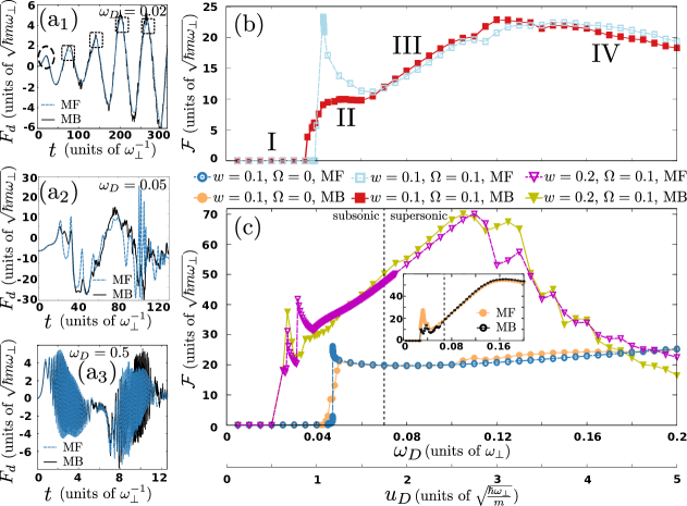
Figure 3: (Color online) $(a_{1})$-$(a_{3})$ Evolution of $F_{d}(t)$ for a full oscillation period for small, intermediate, and large driving frequencies $\omega_{D}$ respectively in both the MF and the MB case. Note that for small and large $\omega_{D}$ the dynamics is well-described by MF theory, while alterations between the two approaches occur at intermediate frequencies. The dashed circle and squares indicate the injection peak and the oscillation maxima respectively. $(b)$ Maximum drag force $\mathcal{F}$ as a function of the driving frequency $\omega_{D}$ in both approaches (see legend). The dynamics is displayed in four regions, namely I-IV (see text). $(c)$ The same as $(b)$ but for different parametric variations and both within the MF and the MB approach (see legend). In all cases $g=1$ and $N=100$, and the second axis used shows the corresponding velocities. Notice here, that the corresponding bulk speed of sound is $c_{0}=1.73$, and thus for $\omega_{D}>0.07$ the impurity is supersonic (vertical dashed line). The inset is the same as $(c)$ but for $g=0.1$ and $B=12$. $A=0.5$ ($A=1$) for $w=0.1$ ($w=0.2$).

III.1 Characterizing the Dissipative Flow via the Drag Force

In order to characterize the superfluid or dissipative flow past the obstacle we invoke the drag force exerted on the fluid by the moving impurity. The drag force Pavloff ; khamis in our inhomogeneous setting is defined as

$$F_{d}(t)=\int^{+\infty}_{-\infty}dx\rho^{(1)}(x;t)\frac{d{V_{D}}}{dx},$$ (5)

where finite drag, $F_{d}\neq 0$, implies dissipation while $F_{d}=0$ corresponds to a superfluid flow. In particular, Figs. 3 $(a_{1})$-$(a_{3})$ illustrate $F_{d}(t)$ during an oscillation period, for small, intermediate, and large driving frequencies respectively. We remark here that from the very early stages of the driving dynamics the drag force acquires a finite value. This is a natural by-product of the moving impurity, as the antisymmetric nature around the impurity center of $\frac{dV_{D}}{dx}$ necessitates a symmetric $\rho^{(1)}(x;t)$ around the impurity in order to vanish. Additionally, and also independently of the value of $\omega_{D}$, a local maximum of $F_{d}(t)$ at $t\approx 25$ is observed in all Figs. 3 $(a_{1})$-$(a_{3})$. The existence of this peak, indicated by a dashed circle in Fig. 3 $(a_{1})$, stems from the fact that the impurity penetrates the BEC from the edge of the Thomas-Fermi radius inducing a density imbalance imprinted in the finite value of the drag force, that would otherwise be absent (e.g. by initializing the impurity from the trap center). For small driving frequencies, e.g. for $\omega_{D}=0.02$ depicted in Fig. 3 $(a_{1})$, $F_{d}(t)$ for $t>25$ undergoes oscillations of increasing amplitude, the maxima of which are indicated by dashed rectangles. This oscillating behavior is directly related with the collective dipole oscillation of the trapped BEC due to the presence of the impurity Kohn ; Albert , and can be removed by subtracting the background density, and further neglecting the contribution of the trap from the definition of Eq. (5), namely $\tilde{F}_{d}=\int^{+\infty}_{-\infty}dx\left[\rho^{(1)}(x;t)-\rho^{(1)}(x;0)\right]\frac{d{V_{G}}}{dx}$. However, this collective motion of the atoms is not related to the onset of dissipation in the system. This result can be directly inferred upon inspecting the corresponding one-body density evolution for small driving frequencies (results not shown here for brevity) which reveals that solitary wave formation is absent during the obstacle’s motion even for larger propagation times. As such in the following we will ignore both the injection peak [namely the first peak in $F_{d}(t)$] as well as the collective oscillation experienced by $F_{d}(t)$ in our calculations, since in the present setup their inclusion is not connected with the onset of dissipation.

Increasing $\omega_{D}$ entails even more rapid oscillations of the corresponding drag force as can be deduced by comparing e.g. Figs. 3 $(a_{2})$, and $(a_{3})$. Notice however, the significantly lower values of $F_{d}(t)$ for large driving frequencies e.g. for $\omega_{D}=0.5$, indicating, as we will trace later on, that for very fast oscillations of the impurity superfluidity is again recovered khamis . In line with these significantly lower values of the drag force it is found that MF theory accurately describes the dynamics both for small (well below unity) and large $\omega_{D}$’s. This result is also directly related and captured by the negligible degree of fragmentation present in the system when considering its MB evolution inside these two parametric windows (see also below).

Differences between the two approaches become significant for intermediate frequencies (or velocities), with the drag force acquiring rather large values reaching a global maximum of the order of $F_{d}(t\approx 80)\approx 18$ ($F_{d}(t\approx 100)\approx 25$) in the MB (MF) approach presented in Fig. 3 $(a_{2})$. It is for this intermediate region that soliton formation takes place, and the critical frequency (or velocity) of its occurrence will be estimated in what follows. The emission of these structures can be identified by the sharp increase of $F_{d}(t)$ and its subsequent decrease as the emitted solitary waves detach from the spatial extent of the impurity.

To shed further light on the above-discussed distinct dynamical regions, and more importantly to evaluate the critical velocity above which the onset of dissipation occurs, we next consider a single crossing of the Gaussian impurity through the BEC. For times $t$ within the interval $t_{1}\in[0,T_{D}/2]$ we evaluate the maximum drag force, $\mathcal{F}\equiv{\rm max}\{F_{d}(t)\}$, exerted on the fluid for varying driving frequencies/velocities and also for different values of the interparticle repulsion $g$ and width $w$ of the impurity. Figs. 3 $(b)$ and $(c)$ summarize our findings. In all cases illustrated in Figs. 3 $(b)$ and $(c)$ and also in both the MF and the MB approach the following general remarks can be made. Four different regions can be identified corresponding roughly to small (I), intermediate (II-III), and large (IV) driving frequencies. For small driving frequencies a plateau of zero drag force is observed–recall that we neglect in this calculation both the injection peak as well as the collective oscillatory motion of the drag force. This plateau is followed by an increase and a subsequent decrease, being more pronounced in the MF approach, of $\mathcal{F}$ for increasing $\omega_{D}$ till almost the end of the subsonic regime ($\omega_{D}\approx 0.07$). Note that the bulk speed of sound, i.e. its maximal value calculated around the center of the trap, is $c_{0}(0)\approx 1.73$ e.g. for $g=1$, and thus for frequencies $\omega_{D}>0.07$ the impurity is supersonic. This decreasing tendency is followed by an almost linear increase of $\mathcal{F}$ that reaches its maximum value within the supersonic regime [see the dashed vertical lines in Fig. 3 $(c)$] dropping down to almost $20\%$ of this maximum for even larger driving frequencies. Overall we can conclude that the small $\omega_{D}$ effect is associated with the motion being too slow, essentially adiabatic and hence solitary waves cannot be generated. On the other hand very large driving frequencies lead to an “averaging out” effect where the oscillation is too fast to excite coherent structures.

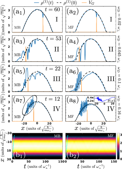
Figure 4: (Color online) ($a_{i}$) Profile snapshots of the one-body density at selected time instants during evolution in all four, I-IV, dynamical regions identified in Fig. 3 both within the MB and the MF approach, with $i=1,\dots,8$ being odd for the former and even for the latter case respectively (see legends). The inset in ($a_{8}$) within the MF approximation, indicates the corresponding phase, $\theta(x)$, to showcase the rapid oscillations of the dispersive sound wave formed. ($b_{1}$) and ($b_{2}$) illustrate the spatiotemporal evolution of the one-body density in the MB and the MF approach respectively for $\omega_{D}=0.5$ when superfluidity is restored. In all cases $g=1$ and $N=100$.

Profile snapshots of both the MB and the MF driving dynamics in each of the above-mentioned regions are illustrated in Figs. 4 $(a_{1})$-$(a_{8})$ for $g=1$. For small driving frequencies (region I) depicted in Figs. 4 $(a_{1})$ and $(a_{2})$ for the MB and the MF case respectively, the flow remains dissipationless during the impurity’s motion until a critical frequency (region II) is reached. The latter is found to be $\omega_{D_{c}}=0.04$ corresponding to a critical velocity $u_{c}/c_{0}\approx 0.57$ within the MF approximation a result that is in excellent agreement with earlier theoretical predictions Hakim , while it is estimated to be $\omega_{D_{c}}=0.036$ (with $u_{c}/c_{0}\approx 0.52$) in the MB scenario. Within this region (II) the flow becomes dissipative imprinted as a sharp jump in $\mathcal{F}$ estimated in the MF case, in contrast to the smoother transition observed in the MB scenario. In particular focusing in the vicinity of the critical point we deduce that dissipation is enhanced in the MB when compared to the MF case. This result is indicated by the higher growth rate of $\mathcal{F}$ in the former approach [see Fig. 3 $(c)$]. Inspecting the MF evolution at $u_{D}\approx u_{c}$ it is found that the solitons are emitted in the low-density region (periphery) of the bosonic cloud Carretero . For increasing $\omega_{D}$, $\mathcal{F}$ exhibits a sharp peak at $\omega_{D}=0.043$, indicating that solitons are emitted also around the trap center. It is this peak that is absent in the MB case which instead showcases a smoother transition (in line with earlier experimental predictions Ketterle_1999 ). This observation further suggests that the critical velocity, estimated to be slightly smaller in the MB case Ketterle_2000 , depends more strongly on the density in the MF case rather than in the MB scenario. The dissipative flow in this region is accompanied by the aforementioned almost periodic emission of downstream gray solitons and upstream dispersive sound waves in both approaches [see e.g. Figs. 4 $(a_{3})$ and $(a_{4})$]. After each soliton emission for a given frequency a decrease in the drag force occurs (which is of course lifted once the soliton travels sufficiently far from the defect, hence the repeated emission observed), while upon further increasing the driving frequency but remaining in region II, leads to the emission of a higher number of coherent structures.

Further increasing the driving frequency, such that the driving becomes supersonic, we enter region III. Here, a coexistence of solitary and dispersive sound waves is observed with the number of the former decreasing gradually while the amplitude of the latter is enhanced [see Figs. 4 $(a_{5})$ and $(a_{6})$ for the MB and the MF outcome respectively]. In both approaches, gray solitons cease to exist for $\omega_{D}\gtrsim 0.12$, namely within region IV where $\mathcal{F}$ reaches also its maximum value, and the dynamics is dominated by significantly amplified sound waves being repeatedly emitted by the obstacle. These sound waves are indicated by the ellipse in Fig. 4 $(a_{7})$. For comparison we also show in this region the corresponding MF profile in Fig. 4 $(a_{8})$. Notice that in this case within this train moving upstream we can distinguish a front and a rapidly oscillatory tail. Inspecting the corresponding phase, $\theta(x)$, shown as an inset in Fig. 4 $(a_{8})$ we observe that it also exhibits an oscillatory behavior. Additionally here, small phase jumps are still imprinted in the phase being connected with the downstream motion of excitations present in the fluid. However these phase jumps correspond to velocities $u_{sol}\gtrsim 0.95c$. It is the presence of these waves that leads to the finite, though much smaller, value of the drag force for the half period driving considered herein, indicating that even for high impurity speeds we do not yet recover superfluidity. The latter is retrieved for even larger driving frequencies than those depicted in Fig. 3 $(c)$ estimated to be $\omega_{D}\gtrsim 0.25$. A case example of the observed dynamics for these large driving frequencies is illustrated in Figs. 4 $(b_{1})$ and $(b_{2})$ for the MB and the MF approach respectively. Indeed in this case we observe that excitations are absent both in the MB and MF cases.

The above distinct dynamical regions (I-IV) are shifted towards smaller or larger $\omega_{D}$ values depending on the characteristics of the obstacle, the spatial inhomogeneity induced by the considered trapping geometry, and on the interaction strength (and thus the speed of sound Ketterle_2000 ). In particular, and as depicted in Fig. 3 $(c)$ larger widths of the Gaussian impurity significantly reduce the critical frequency (velocity) for coherent structure formation e.g. for $w=0.2$ we find that $\omega_{D_{c}}\approx 0.025$ ($u_{c}/c_{0}\approx 0.36$). The oscillatory behavior of $\mathcal{F}$ in this case at intermediate driving frequencies and also in both approaches is related to the fact that the number of solitary waves generated increases dramatically when compared to the $w=0.1$ case. Additionally, the critical velocity is increased in the corresponding homogeneous setting Ketterle_2000 , while for smaller interaction strengths and thus smaller speed of sound again a decrease in the critical velocity is observed [see the inset in Fig. 3 $(c)$]. In particular, in the homogeneous setting the obstacle oscillates in a region of uniform density, resulting to the observed differences in the overall shape of $\mathcal{F}$ in both approaches when compared to the trapped scenario [see Figs. 3 $(b)$ and $(c)$]. In this way, the critical frequency for soliton formation is $\omega_{D_{c}}\approx 0.044$ ($u_{c}/c_{0}\approx 0.64$) in the MB case, and $\omega_{D_{c}}\approx 0.047$ ($u_{c}/c_{0}\approx 0.68$) in the MF approach, leading to a wider region I when compared to the confined case, while all II-IV regions are shifted to even larger $\omega_{D}$ values comment . Note here that for $g=0.1$ deviations between the MF and the MB approaches are negligible for almost every $\omega_{D}$ but in the region of significant solitary wave formation, see e.g. $\omega_{D}\approx 0.03$.

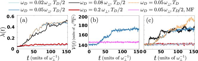
Figure 5: (Color online) $(a)$ Deviation from unity of the first natural population during evolution for different driving frequencies and also for a half and a full oscillation period of the obstacle (see legend). $(b)$ Evolution of the variance $\mathcal{V}(t)$ of a sample of single shots, $N_{shots}=500$, in both the MF and the MB approach (see legend). $(c)$ $\mathcal{V}(t)$ in the MB scenario and for all the cases illustrated in $(a)$. Other parameters used are the same as in Fig 2.

To expose the degree of correlations Mistakidis_per ; Mistakidis_per1 ; negative ; spatial inherent in the system’s evolution, and corresponding departure from the MF regime for the different driving frequency ranges discussed above, we next rely on the deviation from unity of the first natural population, $\lambda(t)=1-n_{1}(t)$. Fig. 5 ($a$) shows $\lambda(t)$ for different $\omega_{D}$’s and $g=1$. Recall that a state with $n_{1}(t)=1$ ($\lambda(t)=0$) is referred to as fully coherent or condensed, while if $n_{i}(t)$ [$\lambda(t)$] significantly deviates from unity [zero] the more modes $n_{i}(t)\neq 0$ ($i=2,3,4$ here) are populated resulting to a fragmented state Penrose ; Mueller . In our setup $\lambda(0)\approx 0.03\neq 0$ holds implying that the initial (ground) state is already depleted. Let us first focus on the driving protocol that refers to half of an oscillation period of the obstacle through the condensate. As time evolves, fragmentation is generally present being more pronounced at moderate driving frequencies residing in regions II and III (see e.g. $\omega_{D}=0.05$) where the structure formation is significant. Contrary to that, for either small (see e.g. $\omega_{D}=0.02$) or large ($\omega_{D}=0.2$) driving frequencies residing respectively in regions I and IV, for which all excitations are absent or the dynamics is dominated by dispersive sound waves, $\lambda(t)$ is significantly suppressed. In all cases the maximum fragmentation rate, identified by the slope $\delta\lambda(t)\equiv\left(\lambda(t+\Delta t)-\lambda(t)\right)/\Delta t$, occurs during the driving (i.e. $t<T_{D}/2$) while after the single crossing of the impurity through the BEC $\lambda(t)$ changes in a far less dramatic manner. Finally, and upon considering the driving dynamics for a complete period of oscillation of the impurity, we observe that $\lambda(t)$ is exactly the same as that resulting from a single obstacle crossing for $0<t\leqslant T_{D}/2$. However, for $t>T_{D}/2$ slight deviations between the free dynamical evolution of the system and the driven one occur.

IV Single-shot simulations

Having discussed the degree of the system’s fragmentation we next showcase how the correlated character of the driven dynamics can be inferred by performing in-situ single-shot absorption measurements lspp ; zorzetos ; Lode which essentially probe the spatial configuration of the atoms being dictated by the MB probability distribution. Relying on the MB wavefunction being available within MCTDHB we emulate the corresponding experimental procedure and simulate such in-situ single-shot images at each instant of the evolution. This simulation procedure is well-established (for more details e.g. see lgspp ; Lode ; kaspar ; Chatterjee ) and therefore it is only briefly outlined below. Referring to the time, $t=t_{im}$, of the imaging we first calculate $\rho^{(1)}(x;t_{im})$ from the MB wavefunction $\ket{\Psi_{N}}\equiv\ket{\Psi_{N}(t_{im})}$. Then, a random position $x^{\prime}_{1}$ is drawn obeying $\rho^{(1)}_{N}(x^{\prime}_{1};t_{im})>l_{1}$ where $l_{1}$ is a random number in the interval [$0$, $\max\{\rho^{(1)}_{N}(x;t_{im})\}$]. Next, one particle located at a position $x^{\prime}_{1}$ is annihilated and the $\rho^{(1)}_{N-1}(x;t_{im})$ is calculated from $\ket{\Psi_{N-1}}$. To proceed, a new random position $x^{\prime}_{2}$ is drawn from $\rho^{(1)}_{N-1}(x;t_{im})$. Following this procedure for $N-1$ steps we obtain the distribution of positions ($x^{\prime}_{1}$, $x^{\prime}_{2}$,…,$x^{\prime}_{N-1}$) which is then convoluted with a point spread function resulting in a single-shot image $\mathcal{A}(\tilde{\textbf{x}})$, where $\tilde{\textbf{x}}$ denote the spatial coordinates within the image. We note that the employed point spread function, being related to the experimental resolution, consists of a Gaussian possessing a width $w=1\ll l\equiv\sqrt{1/\Omega}=10$. $l$ denotes the harmonic oscillator length.

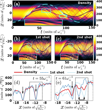
Figure 6: (Color online) $(a)$ Spatio-temporal evolution of the one-body density for $N=10^{4}$ bosons. $(b)$-$(c)$ Evolution of the first and the second in-situ single-shot images respectively. Solid squares and circles indicate the decay events occurring during propagation that are evidently captured by the in-situ single shot images depicted in $(b)$-$(c)$. To better visualize a decay event the insets in ($a$), ($b$), ($c$) depict the spatiotemporal evolution within the region marked by the corresponding square. Profiles of the one-body density and of both shots $(d)$ prior and $(e)$ right after the first decay event marked with squares in $(a)$-$(c)$. Dashed rectangles here indicate the region of interest (see text), while black arrows show the location of the gray solitons formed. Other parameters used are the same as in Fig 2.

To estimate the role of fragmentation from single-shot measurements we utilize their variance for each time instant of the driven dynamics. Below, and unless stated otherwise, we mainly refer to the dynamics induced by the mobile impurity upon considering its single crossing through the condensate, namely for times up to $t_{1}=T_{D}/2$. The variance of a sample of $N_{shots}$ single-shot measurements $\{\mathcal{A}_{k}(\tilde{\textbf{x}})\}_{k=1}^{N_{shots}}$ reads

$$\mathcal{V}(t_{im})=\int d\tilde{\textbf{x}}\frac{1}{N_{shots}}\sum_{k=1}^{N_{shots}}[\mathcal{A}_{k}(\tilde{\textbf{x}};t_{im})-\bar{\mathcal{A}}(\tilde{\textbf{x}};t_{im})]^{2},$$ (6)

where $\bar{\mathcal{A}}(\tilde{\textbf{x}};t_{im})=(1/N_{shots})\sum_{k=1}^{N_{shots}}\mathcal{A}_{k}(\tilde{\textbf{x}};t_{im})$. $\mathcal{V}(t)$ over $N_{shots}=500$ is illustrated in Fig. 5 ($b$) both at the MF and the MB level for $\omega_{D}=0.05$. As it can be deduced in the MF approximation $\mathcal{V}(t)$ remains almost constant exhibiting small amplitude oscillations during evolution. This can be attributed to the fact that for a product MF ansatz all particle detections are independent from each other and the corresponding single-shots of such a state merely reproduce the one-body density (see also the discussion below). In contrast, when correlations are included an overall increase of $\mathcal{V}(t)$ is observed. An increase that is more pronounced during the obstacle’s crossing ($t<T_{D}/2\approx 63$), resembling this way the fragmentation rate $\delta\lambda(t)$ as it can seen by comparing Figs. 5 ($a$) and ($b$). This similarity between the fragmentation process and $\mathcal{V}(t)$ has already been observed in several MB investigations Lode ; lgspp ; lspp and can be explained as follows. Referring to a perfect condensate, i.e. $n_{1}(t)=1$, $\mathcal{V}(t)$ is almost constant during the evolution since all the atoms in the corresponding single-shot measurement are picked from the same SPF $\varphi(t)$ [see the discussion below Eq. (4)]. Contrary to that, for a MB correlated system the corresponding MB state is a superposition of several mutually orthonormal SPFs $\varphi_{i}(t)$, $i=1,...,4$ [see Eq. (3)]. A superposition changes drastically the variance of a sample of single-shots dissociating it from its MF counterpart, since in this case the distribution of the atoms in the cloud depends strongly on the position of the already imaged ones. Moreover, the fact that $\mathcal{V}(t)$ increases during evolution is attributed also to the build-up of higher-order superpositions in the course of the dynamics. To expose further the relation between the growth rate of $\mathcal{V}(t)$ and the fragmentation rate $\delta\lambda(t)$, we present in Fig. 5 ($c$) $\mathcal{V}(t)$ calculated solely in the MB approach for different driving frequencies $\omega_{D}$. The impurity, here, oscillates over $T_{D}/2$ through the ensemble which is then left to evolve. It is observed that $\mathcal{V}(t)$ resembles the increasing tendency of $\lambda(t)$ during evolution for all $\omega_{D}$ regions as can be deduced by comparing Figs. 5 ($a$) and ($c$). For instance, $\mathcal{V}(t)$ is more pronounced for moderate driving frequencies (e.g. $\omega_{D}=0.05$) for which the coherent structure formation is most significant, and becomes lesser in magnitude for either small or large $\omega_{D}$’s (see e.g. $\omega_{D}=0.02$ and $\omega_{D}=0.2$ respectively). Finally, for an impurity oscillating over one period inside the BEC $\mathcal{V}(t)$ grows further for $t>T_{D}/2$ when compared to the situation of a half period of oscillation.

Let us now investigate whether the gray soliton generation, and its subsequent decay and splitting can be observed in an in-situ single-shot image. We remark that a direct observation of the one-body density in a single-shot image is not a-priori possible due to the small particle number, $N=100$, of the considered bosonic gas and the presence of multiple orbitals in the system. Within our treatment the MB state is constructed as a superposition of multiple orbitals [see Eq. (3)] and therefore imaging an atom alters the MB state of the remaining atoms and hence their one-body density. The latter is in direct contrast to a MF state, composed from a single macroscopic orbital, where the imaging of an atom does not affect the distribution of the rest (see also the above discussion of the corresponding variance). Thus in order to fairly capture the spatio-temporal evolution of the one-body density via a single-shot image, we consider the driving dynamics for the oscillating impurity over one period for $\omega_{D}=0.05$ and upon considering a fairly large number of particles, i.e. $N=10^{4}$. The one-body density evolution of this system is shown in Fig. 6 ($a$) where the creation of solitary waves which are prone to decay is observed, as in the case of $N=100$ bosons. Note, however, that the products of a decay event are much less discernible when compared to the $N=100$ particle case [see Fig. 2 ($b_{3}$) and Fig. 6 $(a)$] as here many collision events between the emitted solitons occur which distort the MB evolution. Additionally, the domain wall structures developed between the higher-lying orbitals, though still present, are less apparent, i.e. having significantly lower population, and as such are not clearly imprinted in the one-body density. In this system $g=0.01$ which essentially corresponds to the scaled interaction strength (such that $Ng=const.$) of the $N=100$ with $g=1$ case. Also we note here that the simulation of this system has been performed within a two orbital approximation as the inclusion of further orbitals is computationally prohibitive. Figs. 6 ($b$), ($c$) illustrate the first and the second samples of simulated in-situ single-shot images $\mathcal{A}(\tilde{\textbf{x}})$ for the entire evolution time. It is evident that in both shots the soliton formation takes place, and most importantly their subsequent decay and splitting is observed resembling this way the overall behavior of the one-body density. Case examples of these latter events at different time instants are indicated in Figs. 6 ($b$), ($c$) by light blue squares and circles. For a better visualization of a decay event imprinted in a single-shot image during evolution we provide as an inset the spatiotemporal region indicated by the square. For this magnified region in Figs. 6 ($d$), ($e$) profiles of the one-body density as well as of both shots are illustrated prior (at $t=55$) and after (at time $t=61$) the decay and splitting respectively. Dashed rectangles mark the spatial position of one parent soliton [Fig. 6 ($d$)] which subsequently decays and splits into two daughter ones [Figs. 6 ($e$)] while arrows indicate the locations of all solitons. Notice that before the decay takes place both shots clearly capture the solitons imprinted in the one-body density [see Figs. 6 ($d$)]. Remarkably enough, at later times when the two fragments following the decay of the initial solitary wave are formed, the first shot “picks up” the fragment travelling to the left (with respect to the trap center) while the second shot clearly captures the fragment travelling to the right [see also the inset in Fig. 6 $(a)$]. Importantly here, in both shots the solitons appear much more depleted when compared to the fragments imprinted in the corresponding one-body density which is a clean manifestation of the quantum dispersion of dark soliton’s position that has already been reported in sacha ; sachadark1 . Recalling here that the fragments formed are multi-orbital entities this “pick up” selection observed in the single-shots further implies the presence of domain walls building upon the higher-lying orbitals. Thus, we observe that the single-shot images not only fairly capture the structures building upon the one-body density [in particular compare the insets of Figs. 6 ($a$) and ($b$), ($c$)], but via comparing consecutive shots also signatures of the domain wall structures present can be inferred. Finally, notice that in the corresponding single-shot images the BEC background for evolution times $t>60$ becomes significantly excited and the emergent solitonic structures are hardly discernible. This noise source stems from the increasing shot-to-shot variations due to the presence of fragmentation. Recall that in a correlated system each shot alters the MB state Syrwid_shots .

V Conclusions & Future Work

In the present work the MB dissipative flow of a harmonically confined scalar Bose-Einstein condensate has been investigated, exploring similarities and differences of the latter from the single orbital MF case. To quantify dissipation the drag force exerted on the fluid upon driving an oscillating Gaussian impurity through the bosonic cloud is used as a measure. Distinct dynamical regions are identified corresponding to small, intermediate, and large oscillation frequencies. It is found that for slow (adiabatic) and rapid (averaged out) oscillations of the impurity, MF theory adequately describes the driving dynamics, a result that is clearly captured also by the negligible fragmentation measured in these parameter regions.

However, at moderate driving frequencies (or velocities) fragmentation becomes significant and thus a MB treatment is required. In this region an increase in the maximum of the drag force signals the onset of dissipation. The critical frequency for this transition is found to be slightly smaller and the transition itself smoother when MB effects are taken into account. In particular, the critical velocity for the onset of dissipation and the subsequent solitary wave formation is found to depend on the interaction strength and thus on the corresponding speed of sound Ketterle_1999 ; Ketterle_2000 . It also depends on the trapping geometry, shifting to smaller critical values the breaking of superfluidity when compared to the unconfined case, and finally on the characteristics of the impurity. In this latter case, deviations between the two approaches are much more pronounced as the interparticle interaction is increased, with the critical velocity measured in the MB scenario being shifted to slightly smaller values. Once this critical frequency is reached a spontaneous emission of downstream gray solitons and upstream dispersive sound waves takes place. This emission occurs whenever the impurity’s motion becomes locally supersonic increasing the number of solitary waves generated in an oscillation period. We demonstrate that these states naturally emerge in the MB setting as fundamental excitations of the system. Each of the gray solitary waves formed soon after its generation is found to decay and split into two daughter gray solitary waves that are seen to propagate for large evolution times. Moreover, importantly at later times we identify domain wall states that are unique to the MB phenomenology as they arise between different orbitals. These are reflected into density dips appearing at the one-body density, at first glance, as gray solitons, although a closer inspection of the different orbital densities reveals their domain wall structure. To probe fragmentation we compare its growth rate in this region of moderate frequencies to the growth rate of the variance of a sample of single-shot simulations that are used to complement our findings. Importantly here, upon enlarging the number of particles present in the system the evolution of in-situ single shot images directly dictates not only the generation, but for the first time the decay and splitting of these solitary waves offering evidence that can be experimentally tested. However contrary to the fewer particle scenario, upon enlarging the system the previously robust domain wall structures are no longer clearly imprinted in the one-body density evolution but their presence can be indirectly inferred by comparing consecutive single-shot images. The smearing effect of the domain walls in the one-body density stems from the fact that in this case the coherent structures that are generated after the splitting, suffer multiple collisions with one another as well as with the sound waves present, which significantly excites the background rendering their observation far less straightforward.

Further increasing the driving frequency, there exists a parameter window where both solitons and dispersive sound waves coexist, while for even larger driving frequencies the dynamics is dominated by dispersive sound waves. Finally, it is found that superfluidity is retrieved upon considering very high speed impurities with velocities estimated to be more than six times the bulk speed of sound in the MB approach.

There is a line of interesting directions worth pursuing in future efforts. A straightforward one would be to generalize the current findings in two dimensions where the role of dark solitons is played by vortices. In this case, driving a Gaussian surface through the BEC may give rise to stripe dark states or even transient states such as oblique dark solitons el , whose spontaneous formation and dynamical evolution in a MB environment is yet rather unexplored. Notice that in addition now the spatial width of the driving impurity along the transverse direction will play a role in the emergence (and the resulting nature) of the coherent structures in this system. This latter exploration seems to be particularly timely and relevant, given the use of the motion of laser beams (in the so-called chopsticks method) both theoretically at the MF level bettina , as well as experimentally kali , in order to produce arbitrary vortex configurations in 2D. A related interconnected experimental exploration concerns the also very recently reported formation of the two-dimensional localized Jones-Roberts solitons kaib . Examining whether these structures can be created through such a process at the multi-orbital level and how their MB analogues would dynamically evolve renders this an especially worthwhile direction of near-future work. Additionally, one could also consider the presence of dipolar interactions Bland in the 1D setting and further study the spontaneous generation of nonlinear excitations in such a case, and the subsequent deviations from the dynamics observed herein. Finally, it would be a challenging future task to study how the presented results are altered at finite temperatures burger ; Proukakis and explore how fragmentation competes with thermal effects in MB systems. Since experiments have started exploring more systematically the role of thermally-induced dissipation towards the expulsion of coherent structures such as vortices shinn , addressing such questions also for states such as dark solitons acquires particular timeliness and significance as a topic for future study.

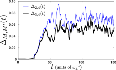
Figure 7: (Color online) $\Delta_{M,M^{\prime}}(t)$ during evolution upon increasing the number of orbitals used (see legend). $\omega_{D}=0.05$ and the driving dynamics corresponds to a full oscillation period of the impurity through the BEC.

Appendix A Ingredients and Covergence of the Many-Body Simulations

In the present Appendix we outline some basic features of our computational method MCTDHB cederbaum1 ; cederbaum2 , discuss the ingredients of our numerical calculations and showcase the convergence of our results. Let us remark that within our implementation we use the Multi-Layer Multi-Configuration Time-Dependent Hartree method for bosonic and fermionic Mixtures (ML-MCTDHX) Cao ; matakias ; moulosx . It is an extended version of the MCTDHB and has been designed for the treatment of multicomponent ultracold systems Katsimiga ; lspp ; BF . We note that for single bosonic species, as is the case considered herein, ML-MCTDHX reduces to MCTDHB.

MCTDHB is a variational method for solving the time-dependent MB Schrödinger equation of interacting bosonic systems. It relies on expanding the total MB wavefunction with respect to a time-dependent and variationally optimized basis, which enables us to capture the important correlation effects using a computationally feasible basis size. Namely, it allows us to span more efficiently the relevant, for the system under consideration, subspace of the Hilbert space at each time instant with a reduced number of basis states when compared to expansions relying on a time-independent basis. In particular, the MB wavefunction of $N$ bosons is expressed by a linear combination of time-dependent permanents $\ket{\vec{n}}=\left|{{n_{1}},{n_{2}},...,{n_{M}};t}\right\rangle$ with time-dependent expansion coefficients $A_{\vec{n}}(t)$. These permanents build upon $M$ time-dependent single-particle functions $\ket{\varphi_{i}(t)}$, $i=1,\dots,M$ which are expanded within a time-independent primitive basis $\{\ket{k}\}$ of dimension $\mathcal{M}$. We note here that for $M=1$ the MB wavefunction is given by a single permanent $\ket{n_{1}=N;t}$ and the method reduces to the time-dependent Gross-Pitaevskii MF approximation.

For our simulations, we use a primitive basis consisting of a sine discrete variable representation with $\mathcal{M}=1500$ grid points. To perform the simulations into a finite spatial region, we impose hard-wall boundary conditions at the positions $x_{\pm}=\pm 80$. The Thomas-Fermi radius of the bosonic cloud is of the order of $R_{TF}\sim 25$ for $g=1$ and $R_{TF}\sim 12$ for $g=0.1$. The location of the imposed boundary conditions does not affect our results as we never observe appreciable densities beyond $x=\pm 35$. To achieve numerical convergence, we ensure that the expectation value of the observables of interest become to a certain degree insensitive when increasing the number of basis states. Regarding our simulations we have used $M=4$ orbitals. To quantify the degree of convergence, for instance, of the one-body density evolution we invoke the spatially integrated difference between the $M$ and $M^{\prime}$ orbital configurations

$$\Delta_{M^{\prime},M}(t)=\frac{\int_{x_{-}}^{x_{+}}dx|\rho_{M^{\prime}}^{(1)}(x,t)-\rho_{M}^{(1)}(x,t)|}{\int_{x_{-}}^{x_{+}}dx\rho_{M}^{(1)}(x,t)}.$$ (7)

Fig. 7 shows both $\Delta_{2,4}(t)$ and $\Delta_{3,4}(t)$ during the evolution upon considering the driving of the impurity through the BEC for an oscillation period, for $\omega_{D}=0.05$ lying within region II where fragmentation becomes significant. A systematic convergence of $\Delta_{M,M^{\prime}}(t)$ is showcased for increasing the number of orbitals. As it is evident $\Delta_{3,4}(t)$ testifies negligible deviations between the two orbital configurations, becoming at most $7\%$ at large evolution times ($t>100$), in contrast to the larger deviations observed in $\Delta_{2,4}(t)$ during evolution.

References

- (1) V. E. Zakharov, and A. B. Shabat, Sov. Phys. JETP 37, 823 (1973).
- (2) J. F. Corney, P. D. Drummond, and A. Liebman, Opt. Commun. 140, 211 (1997).
- (3) Y. S. Kivshar, and D. Luther-Davies, Phys. Rep. 298, 81 (1998).
- (4) C. J. Pethick and H. Smith, Bose-Einstein condensation in dilute gases, Cambridge University Press (Cambridge, 2002).
- (5) L. P. Pitaevskii, and S. Stringari, Bose-Einstein Condensation, Oxford University Press (Oxford, 2003).
- (6) D. J. Frantzeskakis, J. Phys. A Math. Theor. 43, 213001 (2010).
- (7) P. G. Kevrekidis, D. J. Frantzeskakis, and R. Carretero-González, The Defocusing Nonlinear Schrödinger Equation, SIAM (Philadelphia, 2015).
- (8) A. Chabchoub, O. Kimmoun, H. Branger, N. Hoffmann, D. Proment, M. Onorato, and N. Akhmediev, Phys. Rev. Lett. 110, 124101 (2013).
- (9) W. Tong, M. Wu, L. D. Carr, and B. A. Kalinikos, Phys. Rev. Lett. 104, 037207 (2010).
- (10) S. Burger, K. Bongs, S. Dettmer, W. Ertmer, K. Sengstock, A. Sanpera, G. Shlyapnikov, and M. Lewenstein, Phys. Rev. Lett. 83, 5198 (1999).
- (11) J. Denschlag, J. E. Simsarian, D. L. Feder, C. W. Clark, L. A. Collins, J. Cubizolles, L. Deng, E. W. Hagley, K. Helmerson, W. P. Reinhardt, S. L. Rolston, B. I. Schneider, and W. D. Phillips, Science 287, 97 (2000).
- (12) C. Becker, S. Stellmer, P. Soltan-Panahi, S. Dörscher, M. Baumert, E.-M. Richter, J. Kronjäger, K. Bongs, and K. Sengstock, Nat. Phys. 4, 496 (2008).
- (13) A. Weller, J. P. Ronzheimer, C. Gross, J. Esteve, M. K. Oberthaler, D. J. Frantzeskakis, G. Theocharis, and P. G. Kevrekidis, Phys. Rev. Lett. 101, 130401 (2008).
- (14) G. Theocharis, A. Weller, J. P. Ronzheimer, C. Gross, M. K. Oberthaler, P. G. Kevrekidis, and D. J. Frantzeskakis, Phys. Rev. A 81, 063604 (2010).
- (15) W. P. Reinhardt, and C. W. Clark, J. Phys. B 30, L785 (1997).
- (16) T. F. Scott, R. J. Ballagh, and K. Burnett, J. Phys. B 31, L329 (1998).
- (17) Z. Dutton, M. Budde, C. Slowe, and L. V. Hau, Science 293, 663 (2001).
- (18) P. Engels, and C. Atherton, Phys. Rev. Lett. 99, 160405 (2007).
- (19) Vincent Hakim, Phys. Rev. E 55, 2835 (1997).
- (20) P. Leboeuf, and N. Pavloff, Phys. Rev. A 64, 033602 (2001).
- (21) N. Pavloff, Phys. Rev. A 66, 013610 (2002).
- (22) V. A. Brazhnyi, and A. M. Kamchatnov, Phys. Rev. A 68, 043614 (2003).
- (23) Abdelaziz Radouani, Phys. Rev. A 70, 013602 (2004).
- (24) R. Carretero-González, P. G. Kevrekidis, D. J. Frantzeskakis, B. A. Malomed, S. Nandi, and A. R. Bishop, Math. Comput. Simul. 74 361 (2007).
- (25) I. Hans, J. Stockhofe, and P. Schmelcher, Phys. Rev. A 92, 013627 (2015).
- (26) M. Syafwan, P. Kevrekidis, A. Paris-Mandoki, I. Lesanovsky, P. Krüger, L. Hackermuller, and H. Susanto, J. Phys. B: At. Mol. Opt. Phys. 49, 235301 (2016).
- (27) T. Frisch, Y. Pomeau, and S. Rica, Phys. Rev. Lett. 69, 1644 (1992).
- (28) T. Winiecki, J. F. McCann, and C. S. Adams, Phys. Rev. Lett. 82, 5186 (1999).
- (29) G. E. Astrakharchik, and L. P. Pitaevskii, Phys. Rev. A 70, 013608 (2004).
- (30) L. D. Landau, J. Phys. (Moscow) 5, 71 (1941).
- (31) C. Raman, M. Köhl, R. Onofrio, D. S. Durfee, C. E. Kuklewicz, Z. Hadzibabic, and W. Ketterle, Phys. Rev. Lett. 83, 2502 (1999).
- (32) R. Onofrio, C. Raman, J. M. Vogels, J. R. Abo-Shaeer, A. P. Chikkatur, and W. Ketterle, Phys. Rev. Lett. 85, 2228 (2000).
- (33) A. M. Kamchatnov, and N. Pavloff, Phys. Rev. A 85, 033603 (2012).
- (34) G. A. El, and A. M. Kamchatnov, Phys. Lett. A 350, 192 (2006).
- (35) G. A. El, A. M. Kamchatnov, V. V. Khodorovskii, E. S. Annibale, and A. Gammal, Phys. Rev. E 80, 046317 (2009).
- (36) M. A. Hoefer, and B. Ilan, Phys. Rev. A 80, 061601(R) (2009).
- (37) G.A. El, M.A. Hoefer, Physica D 333, 11 (2016).
- (38) C. Huepe, and M. -E. Brachet, C. R. Acad. Sci. Paris 325, 195 (1997).
- (39) J. Dziarmaga, and K. Sacha, Phys. Rev. A 66, 043620 (2002).
- (40) J. Dziarmaga, Z. P. Karkuszewski, and K. Sacha, Phys. Rev. A 66, 043615 (2002).
- (41) J. Dziarmaga, Z. P. Karkuszewski, and K. Sacha, J. Phys. B: At. Mol. Opt. Phys. 36, 1217 (2003).
- (42) R. V. Mishmash, and L. D. Carr, Phys. Rev. Lett. 103, 140403 (2009).
- (43) R. V. Mishmash, I. Danshita, C. W. Clark, and L. D. Carr, Phys. Rev. A 80, 053612 (2009).
- (44) A. D. Martin, and J. Ruostekoski, Phys. Rev. Lett. 104, 194102 (2010).
- (45) D. Delande, and K. Sacha, Phys. Rev. Lett. 112, 040402 (2014).
- (46) A. Syrwid, and K. Sacha, Phys. Rev. A 96, 043602 (2017).
- (47) G. C. Katsimiga, G. M. Koutentakis, S. I. Mistakidis, P. G. Kevrekidis, and P. Schmelcher, New J. Phys. 19, 073004 (2017).
- (48) S. I. Mistakidis, G. C. Katsimiga, P. G. Kevrekidis, and P. Schmelcher, New J. Phys. 20, 043052 (2018).
- (49) G. C. Katsimiga, G. M. Koutentakis, S. I. Mistakidis, P. G. Kevrekidis, and P. Schmelcher, New J. Phys. 19, 123012 (2017).
- (50) K. C. Wright, R. B. Blakestad, C. J. Lobb, W. D. Phillips, and G. K. Campbell, Phys. Rev. Lett. 110, 025302 (2013).
- (51) C. Ryu, P. W. Blackburn, A. A. Blinova, and M. G. Boshier, Phys. Rev. Lett. 111, 205301 (2013).
- (52) S. Eckel, J. G. Lee, F. Jendrezejewski, N. Murray, C. W. Clark, C. J. Lobb, W. D. Phillips, M. Edwards, and C. K. Campbell, Nat. 506, 200 (2014).
- (53) F. Jendrezejewski, S. Eckel, N. Murray, C. Lanier, M. Edwards, C. J. Lobb, and C. K. Campbell, Phys. Rev. Lett. 113, 045305 (2014).
- (54) W. Weimer, K. Morgener, V. P. Singh, J. Siegl, K. Hueck, N. Luick, L. Mathey, and H. Moritz, Phys. Rev. Lett. 114, 095301 (2015).
- (55) A. Burchianti, F. Scazza, A. Amico, G. Valtolina, J. A. Seman, C. Fort, M. Zaccanti, M. Inguscio, and G. Roati, Phys. Rev. Lett. 120, 025302 (2018).
- (56) G. Theocharis, P.G. Kevrekidis, H.E. Nistazakis, D.J. Frantzeskakis, A.R. Bishop, Phys. Lett. A 337, 441 (2005).
- (57) P. O. Fedichev, and G. V. Shlyapnikov, Phys. Rev. A 63, 045601 (2001).
- (58) S.I. Mistakidis, and P. Schmelcher, Phys. Rev. A 95, 013625 (2017).
- (59) S.I. Mistakidis, T. Wulf, A. Negretti, and P. Schmelcher, J. Phys. B: At. Mol. Opt. Phys. 48, 244004 (2015).
- (60) O. E. Alon, A. I. Streltsov, and L. S. Cederbaum, J. Chem. Phys. 127, 154103 (2007).
- (61) O. E. Alon, A. I. Streltsov, and L. S. Cederbaum, Phys. Rev. A 77, 033613 (2008).
- (62) E. G. Khamis, and A. Gammal, Phys. Rev. A 87, 045601 (2013).
- (63) M. Kato, X. -F. Zhang, and H. Saito, Phys. Rev. A 96, 033613 (2017).
- (64) F. Pinsker, Physica B: Cond. Mat. 521, 36 (2017).
- (65) A. Paris-Mandoki, J. Shearring, F. Mancarella, T. M. Fromhold, A. Trombettoni, and P. Krüger, Sc. Rep. 7, 9070 (2017).
- (66) M. Olshanii, Phys. Rev. Lett. 81, 938 (1998).
- (67) S. Inouye, M. R. Andrews, J. Stenger, H.-J. Miesner, D. M. Stamper-Kurn, and W. Ketterle, Nat. 392, 151 (1998).
- (68) C. Chin, R. Grimm, P. Julienne, and E. Tiesinga, Rev. Mod. Phys. 82, 1225 (2010).
- (69) L. Cao, S. Krönke, O. Vendrell, and P. Schmelcher, J. Chem. Phys., 139, 134103 (2013).
- (70) S. Krönke, L. Cao, O. Vendrell, and P. Schmelcher, New J. Phys. 15, 063018 (2013).
- (71) L. Cao, V. Bolsinger, S. I. Mistakidis, G. M. Koutentakis, S.Krönke, J. M. Schurer, and P. Schmelcher, J. Chem. Phys. 147, 044106 (2017).
- (72) A. D. McLachlan, Mol. Phys. 8, 39 (1964).
- (73) U. M. Titulaer, and R. J. Glauber, Phys. Rev. 140, 676 (1965).
- (74) M. Naraschewski, and R. J. Glauber, Phys. Rev. A 59, 4595 (1999).
- (75) K. Sakmann, A. I. Streltsov, O. E. Alon, and L. S. Cederbaum, Phys. Rev. A 78, 023615 (2008).
- (76) O. Penrose, and L. Onsager, Phys. Rev. 104, 576 (1956).
- (77) E. J. Mueller, T. L. Ho, M. Ueda, and G. Baym, Phys. Rev. A 74, 33612 (2006).
- (78) M. Trippenbach, K. Góral, K. Rza̧żewski, B. A. Malomed, and Y. B. Band, J. Phys. B: At. Mol. Opt. Phys. 33, 4017 (2000).
- (79) W. Kohn, Phys. Rev. 123, 1242 (1961).
- (80) M. Albert, T. Paul, N. Pavloff, and P. Leboeuf, Phys. Rev. Lett. 100, 250405 (2008).
- (81) Note that in the homogeneous setting the speed of sound, , is uniform. Thus, in order to reach region IV the velocity of the obstacle at the initial stages of the dynamics must be much larger than resulting to a downstream emission of excitations with velocities comparable to .
- (82) S.I. Mistakidis, L. Cao, and P. Schmelcher, Phys. Rev. A 91, 033611 (2015).
- (83) T. Plaßmann, S.I. Mistakidis, and P. Schmelcher, arXiv:1802.06693 (2018).
- (84) G.M. Koutentakis, S.I. Mistakidis, and P. Schmelcher, arXiv:1804.07199 (2018).
- (85) A. U. Lode, and C. Bruder, Phys. Rev. Lett. 118, 013603 (2017).
- (86) K. Sakmann, and M. Kasevich, Nat. Phys. 12, 451 (2016).
- (87) B. Chatterjee, and A. U. Lode, arXiv:1708.07409 (2017).
- (88) A. Syrwid, M. Brewczyk, M. Gajda, and K. Sacha, Phys. Rev. A 94, 023623 (2016).
- (89) G. A. El, A. Gammal, and A. M. Kamchatnov, Phys. Rev. Lett. 97, 180405 (2006).
- (90) B. Gertjerenken, P. G. Kevrekidis, R. Carretero-González, and B. P. Anderson, Phys. Rev. A 93, 023604 (2016).
- (91) E. C. Samson, K. E. Wilson, Z. L. Newman, and B. P. Anderson, Phys. Rev. A 93, 023603 (2016).
- (92) N. Meyer, H. Proud, M. Perea-Ortiz, C. O’Neale, M. Baumert, M. Holynski, J. Kronjäger, G. Barontini, and K. Bongs, Phys. Rev. Lett. 119, 150403 (2017).
- (93) T. Bland, K. Pawłowski, M. J. Edmonds, K. Rza̧żewski, and N. G. Parker, Phys. Rev. A 95, 063622 (2017).
- (94) B. Jackson, N. P. Proukakis, and C. F. Barenghi, Physical Review A, 75, 051601 (2007).
- (95) G. Moon, W.J. Kwon, H. Lee, Y. Shin, Physical Review A 92, 051601(R) (2015).
- (96) P. Siegl, S. I. Mistakidis, and P. Schmelcher, Phys. Rev. A 97, 053626 (2018).