Pion condensation and phase diagram in the Polyakov-loop quark-meson model

Abstract

We use the Polyakov-loop extended two-flavor quark-meson model as a low-energy effective model for QCD to study the phase diagram in the $\mu_{I}$–$T$ plane where $\mu_{I}$ is the isospin chemical potential. In particular, we focus on the Bose condensation of charged pions. At $T=0$, the onset of pion condensation is at $\mu_{I}={1\over 2}m_{\pi}$ in accordance with exact results. The phase transition to a Bose-condensed phase is of second order for all values of $\mu_{I}$ and in the $O(2)$ universality class. The chiral critical line joins the critical line for pion condensation at a point whose position depends on the Polyakov-loop potential and the sigma mass. For larger values of $\mu_{I}$ these curves are on top of each other. The deconfinement line enters smoothly the phase with the broken $O(2)$ symmetry. We compare our results with recent lattice simulations and find overall good agreement.

I Introduction

The phases of QCD as functions of the baryon chemical potential $\mu_{B}$ or the quark chemical potential $\mu={1\over 3}\mu_{B}$, and temperature $T$ have been studied in detail since the first phase diagram was proposed more than fourty years ago raja ; alford ; fukurev . At vanishing baryon chemical potential, it is possible to perform lattice simulations to calculate the thermodynamic functions and the transition temperature associated with chiral symmetry restoration and deconfinement. For physical quark masses and two flavors, the transition is a crossover at a temperature of approximately 155 MeV lat1 ; lat2 ; lat3 ; lat4 .

At nonzero baryon chemical potential, however, Monte Carlo simulations are hampered by the so-called sign problem, namely that the fermion determinant becomes complex. Being complex, the usual interpretation of it as part of a probability distribution can no longer be upheld. The sign problem in QCD at finite baryon density has spurred the interest in QCD-like theories free of this problem. This includes QCD with quarks in the adjoint representation qcdlike1 , two-color QCD qcdlike2 , QCD at finite isospin $\mu_{I}$ son , and QCD in a magnetic field $B$ bali . These theories are all interesting in their own right; QCD at finite isospin and QCD in a magnetic field are also relevant for compact stars. In addition, the application of Monte-Carlo methods allows a direct test of various model approaches in the cases mentioned above. Such a confrontation of model calculations with lattice simulations of QCD in a magnetic field has been very fruitful in understanding their strengths and limitations dimi ; rw .

Lattice simulations of QCD at finite isospin have been performed in e.g. Refs. kogut1 ; kogut2 ; gergy1 ; gergy2 ; gergy3 with particular emphasis on Bose condensation of charged pions for isospin chemical potentials above the zero-temperature critical value $\mu_{I}^{c}={1\over 2}m_{\pi}$. Chiral perturbation theory (ChPT) son ; kim ; loewe ; fragaiso ; carigchpt , which is a model-independent low-energy theory for QCD valid at low densities has been used to study pion condensation. ChPT predicts a second-order transition, which is in agreement with lattice simulations. There have also been a number of other approaches and model calculations studying various aspects of the QCD phase diagram at finite isospin density, including the resonance gas model restoublan , random matrix models random , the Nambu-Jona-Lasinio (NJL) model 2fbuballa ; toublannjl ; bar2f ; he2f ; heman2 ; heman ; ebert1 ; ebert2 ; sun ; lars ; 2fabuki ; heman3 ; he3f , the quark-meson (QM) model lorenz ; ueda ; qmstiele ; patrick , and effective theory at asymptotically high isospin isohigh .

Finally, we mention that one expects another phase transition at large isospin chemical potential. In perturbation theory, one-gluon exchange gives rise to an effective attractive interaction between $u$ and $\bar{d}$ quarks leading to the formation of Cooper pairs son . The transition from a Bose-Einstein condensate (BEC) to a Bardeen-Cooper-Schrieffer (BCS) state is expected to be an analytical crossover as the symmetry-breaking pattern is the same.

As pointed out in Ref. lorenz , there is a mapping of the quark-meson model at finite isospin and the corresponding two-color quark-meson-diquark model at finite baryon chemical potential. The neutral pion $\pi_{0}$ is replaced by an isovector triplet ${\bm{\pi}}$. The charged pions $\pi^{\pm}$ are replaced by a diquark-antidiquark pair $\Delta$ and $\Delta^{*}$, which instead of being coupled to $\mu_{I}$ is now coupled to a baryon chemical potential $\mu_{B}$. Since the gauge groups $SU(2)$ and $SU(3)$ are fundamentally different, this mapping is valid for the matter sector; once we couple the QM model to the Polyakov loop, this identification is lost.

In the present paper, we study the QCD phase diagram at finite temperature and isospin density using the PQM model. The main conclusions of our work are

1. The second order transition to a BEC state. The transition is in the $O(2)$ universality class. At $T=0$, the transition is exactly at $\mu_{I}={1\over 2}m_{\pi}$.

2. The BEC and chiral transition lines meet at a point $(\mu_{I}^{\rm meet},T^{\rm meet})$ and coincide for larger isospin chemical potentials $\mu_{I}$.

3. The deconfinement and chiral transition lines coincide in the non-condensed phase for a logarithmic Polyakov-loop potential and a sufficiently low sigma mass.

4. The deconfinement line penetrates smoothly into the symmetry-broken phase.

These results are in agreement with the recent lattice simulations of Refs. gergy1 ; gergy2 ; gergy3 .

The paper is organized as follows. In Sec. II, we briefly discuss the quark-meson model and in Sec. III we calculate the effective potential in the mean-field approximation. In Sec. IV, we discuss the coupling to the Polyakov loop, while in Sec. V, we present the phase diagram in the $\mu_{I}$–$T$ plane and compare it to recent lattice results. In Appendix A, we list a few integrals needed in the calculations, while Appendix B provides the reader with some details of how the parameters of the quark-meson model are determined.

II Quark-meson model

The Lagrangian of the two-flavor quark-meson model in Minkowski space is

$${\cal L} = {1\over 2}\left[(\partial_{\mu}\sigma)(\partial^{\mu}\sigma)+(\partial_{\mu}\pi_{3})(\partial^{\mu}\pi_{3})\right]$$ (1)

$$+(\partial_{\mu}+2i\mu_{I}\delta_{\mu}^{0})\pi^{+}(\partial^{\mu}-2i\mu_{I}\delta_{0}^{\mu})\pi^{-}$$

$$-{1\over 2}m^{2}(\sigma^{2}+\pi_{3}^{2}+2\pi^{+}\pi^{-})-{\lambda\over 24}(\sigma^{2}+\pi_{3}^{2}+2\pi^{+}\pi^{-})^{2}$$

$$+h\sigma+\bar{\psi}\left[i/\!\!\!\partial+\mu_{f}\gamma^{0}-g(\sigma+i\gamma^{5}{\bm{\tau}}\cdot{\bm{\pi}})\right]\psi\;,$$

where $\psi$ is a color $N_{c}$-plet, a four-component Dirac spinor as well as a flavor doublet

$$\psi = \left(\begin{array}[]{c}u\\ d\end{array}\right)\;,$$ (4)

and $\mu_{f}={\rm diag}(\mu_{u},\mu_{d})$, where $\mu_{u}$ and $\mu_{d}$, are the quark chemical potentials, $\mu_{I}$ is the isospin chemical potential, $\tau_{i}$ ($i=1,2,3$) are the Pauli matrices in flavor space, ${\bm{\pi}}=(\pi_{1},\pi_{2},\pi_{3})$, and $\pi^{\pm}={1\over\sqrt{2}}(\pi_{1}\pm i\pi_{2})$.

Apart from the global $SU(N_{c})$ symmetry, the Lagrangian (1) has a $U(1)_{B}\times SU(2)_{L}\times SU(2)_{R}$ symmetry for $h=0$ and a $U(1)_{B}\times SU(2)_{V}$ symmetry for $h\neq 0$. When $\mu_{u}\neq\mu_{d}$, this symmetry is reduced to $U(1)_{B}\times U_{I_{3}L}(1)\times U_{I_{3}R}(1)$ for $h=0$ and $U(1)_{B}\times U_{I_{3}}(1)$ for $h\neq 0$.

The number density associated with a chemical potential $\mu_{A}$ is

$$n_{A} = -{\partial V\over\partial\mu_{A}}\;,$$ (5)

where $V$ is the effective potential. The baryon and isospin densities can be expressed in terms of the quark densities $n_{u}$ and $n_{d}$ as

$$n_{B} = {1\over 3}(n_{u}+n_{d})\;,$$ (6)

$$n_{I} = n_{u}-n_{d}\;.$$ (7)

Eqs. (6)–(7) together with the chain rule can be used to derive relations among the baryon and isospin chemical potentials and the quark chemical potentials. We have

$$n_{I} = -{\partial V\over\partial\mu_{I}}$$ (8)

$$= -\left({\partial V\over\partial\mu_{u}}-{\partial V\over\partial\mu_{d}}\right)$$

$$= -\left({\partial\mu_{u}\over\partial\mu_{I}}{\partial V\over\partial\mu_{u}}+{\partial\mu_{d}\over\partial\mu_{I}}{\partial V\over\partial\mu_{d}}\right)\;.$$

This yields

$${\partial\mu_{u}\over\partial\mu_{I}}=-{\partial\mu_{d}\over\partial\mu_{I}}=1\;.$$ (9)

Similarly, we find ${\partial\mu_{u}\over\partial\mu_{B}}={\partial\mu_{d}\over\partial\mu_{B}}={1\over 3}$. From this, we find the following relations among the chemical potentials

$$\mu_{u} = {1\over 3}\mu_{B}+\mu_{I}\;,$$ (10)

$$\mu_{d} = {1\over 3}\mu_{B}-\mu_{I}\;.$$ (11)

Introducing the quark chemical potential $\mu={1\over 3}\mu_{B}$ and inverting the relations (10)–(11), we find

$$\mu = {1\over 2}(\mu_{u}+\mu_{d})\;,$$ (12)

$$\mu_{I} = {1\over 2}(\mu_{u}-\mu_{d})\;.$$ (13)

III Effective potential

The expectation values of the fields are written as

$$\sigma = \phi_{0}\;,\hskip 14.22636pt\pi_{1}=\pi_{0}\;,$$ (14)

where $\phi_{0}$ and $\pi_{0}$ are constant in space. The former is the usual chiral condensate, while the latter represents a homogeneous pion condensate. A pion condensate breaks the $U_{I_{3}L}(1)\times U_{I_{3}R}(1)$ symmetry to $U_{I_{3}V}(1)$ or the $U_{I_{3}}(1)$ symmetry. Introducing $\Delta=g\phi_{0}$ and $\rho=g\pi_{0}$, the tree-level potential in Euclidean space can be written as

$$V_{0} = {1\over 2}{m^{2}\over g^{2}}\Delta^{2}+{1\over 2}{m^{2}-4\mu_{I}^{2}\over g^{2}}\rho^{2}$$ (15)

$$+{\lambda\over 24g^{4}}\left(\Delta^{2}+\rho^{2}\right)^{2}-{h\over g}\Delta\;.$$

Expressing the parameters in Eq. (1) terms of the sigma mass $m_{\sigma}$, the pion mass $m_{\pi}$, the pion decay constant $f_{\pi}$, and the constituent quark mass $m_{q}$ , we find

$$m^{2} = -{1\over 2}\left(m_{\sigma}^{2}-3m_{\pi}^{2}\right)\;,\,\lambda=3{\left(m_{\sigma}^{2}-m_{\pi}^{2}\right)\over f_{\pi}^{2}}\;,$$ (16)

$$g^{2} = {m_{q}^{2}\over f_{\pi}^{2}}\;,\hskip 59.75095pth=m_{\pi}^{2}f_{\pi}\;.$$ (17)

Inserting these relations, we can write the tree-level potential as

$$V_{0} = -{1\over 4}f_{\pi}^{2}(m_{\sigma}^{2}-3m_{\pi}^{2}){\Delta^{2}+\rho^{2}\over m_{q}^{2}}-2\mu_{I}^{2}f_{\pi}^{2}{\rho^{2}\over m_{q}^{2}}$$ (18)

$$+{1\over 8}f_{\pi}^{2}(m_{\sigma}^{2}-m_{\pi}^{2}){(\Delta^{2}+\rho^{2})^{2}\over m_{q}^{4}}-m_{\pi}^{2}f_{\pi}^{2}{\Delta\over m_{q}}\;.$$

The quark energies can be read off from the zeros of the determinant of the Dirac operator. One finds

$$E_{u} = E(-\mu_{I})\;,\hskip 28.45274ptE_{d}=E(\mu_{I})\;,$$ (19)

$$E_{\bar{u}} = E(\mu_{I})\;,\hskip 35.56593ptE_{\bar{d}}=E(-\mu_{I})\;.$$ (20)

where we have defined

$$E(\mu_{I}) = \left[\left(\sqrt{p^{2}+\Delta^{2}}+{\mu_{I}}\right)^{2}+\rho^{2}\right]^{1\over 2}\;.$$ (21)

Note that the quark energies explicitly depend on $\mu_{I}$. In the following we choose $\mu_{I}>0$, but similar results are obtained for $\mu_{I}<0$.

The one-loop contribution to the effective potential at $T=\mu_{B}=0$ is

$$V_{1} = -N_{c}\int_{p}\left(E_{u}+E_{d}+E_{\bar{u}}+E_{\bar{d}}\right)\;,$$ (22)

where the integral is in $d=3-2\epsilon$ dimensions (See Appendix A). The integral in Eq. (22) is ultraviolet divergent and in order to isolate the divergences, we need to expand the energies in powers of $\mu_{I}$ to the appropriate order. This yields

$$V_{\rm div} = -4N_{c}\int_{p}\left[\sqrt{p^{2}+\Delta^{2}+\rho^{2}}+{\mu_{I}^{2}\rho^{2}\over 2({p^{2}+\Delta^{2}+\rho^{2})^{3\over 2}}}\right]={4N_{c}\over(4\pi)^{2}}\left({e^{\gamma_{E}}\Lambda^{2}\over\Delta^{2}+\rho^{2}}\right)^{\epsilon}\left[\left(\Delta^{2}+\rho^{2}\right)^{2}\Gamma(-2+\epsilon)-2\mu_{I}^{2}\rho^{2}\Gamma(\epsilon)\right]\;.$$

The remainder $V_{\rm fin}$ is finite and reads

$$V_{\rm fin} = V_{1}-V_{\rm div}\;.$$ (24)

Note that $V_{\rm fin}$ can be evaluated directly in $d=3$ dimensions. In the present case, $V_{\rm fin}$ must be evaluated numerically. Using the expressions for the integrals listed in Appendix A, we can write the unrenormalized one-loop effective potential $V=V_{0}+V_{1}$ as

$$V = {1\over 2}{m^{2}\over g^{2}}\Delta^{2}+{1\over 2}{m^{2}-4\mu_{I}^{2}\over g^{2}}\rho^{2}+{\lambda\over 24g^{4}}(\Delta^{2}+\rho^{2})^{2}-{h\over g}\Delta$$ (25)

$$+{2N_{c}\over(4\pi)^{2}}\left(\Lambda^{2}\over\Delta^{2}+\rho^{2}\right)^{\epsilon}\left[\left(\Delta^{2}+\rho^{2}\right)^{2}\left({1\over\epsilon}+{3\over 2}\right)-4\mu_{I}^{2}\rho^{2}{1\over\epsilon}\right]+V_{\rm fin}+{\cal O}(\epsilon)\;,$$

which contains poles in $\epsilon$. These poles are removed by mass and coupling constant renormalization. In the $\overline{\rm MS}$ scheme this is achieved by making the substitutions $m^{2}\rightarrow Z_{m^{2}}m^{2}$, $\lambda\rightarrow Z_{\lambda}\lambda$, $g^{2}\rightarrow Z_{g^{2}}g^{2}$, and $h\rightarrow Z_{h}h$, where

$$Z_{m^{2}}=1+{4N_{c}g^{2}\over(4\pi)^{2}\epsilon}\;,\hskip 11.38092ptZ_{\lambda}=1+{8N_{c}\over(4\pi)^{2}\epsilon}\left[g^{2}-6{g^{4}\over\lambda}\right]\;,\hskip 11.38092ptZ_{g^{2}}=1+{4N_{c}g^{2}\over(4\pi)^{2}\epsilon}\;,\hskip 11.38092ptZ_{h}=1+{2N_{c}g^{2}\over(4\pi)^{2}\epsilon}\;,\hskip 11.38092pt$$ (26)

The renormalized one-loop effective potential then reads

$$V_{\rm 1-loop} = {1\over 2}{m^{2}_{\overline{\text{\tiny MS}}}\over g^{2}_{\overline{\text{\tiny MS}}}}\Delta^{2}+{1\over 2}{m^{2}_{\overline{\text{\tiny MS}}}-4\mu_{I}^{2}\over g^{2}_{\overline{\text{\tiny MS}}}}\rho^{2}+{\lambda_{\overline{\text{\tiny MS}}}\over 24g_{\overline{\text{\tiny MS}}}^{4}}\left(\Delta^{2}+\rho^{2}\right)^{2}-{h_{\overline{\text{\tiny MS}}}\over g_{\overline{\text{\tiny MS}}}}\Delta$$ (27)

$$+{2N_{c}\over(4\pi)^{2}}\Bigg{\{}\left[\left(\Delta^{2}+\rho^{2}\right)^{2}-4\mu_{I}^{2}\rho^{2}\right]\log\left({\Lambda^{2}\over\Delta^{2}+\rho^{2}}\right)+{3\over 2}\left(\Delta^{2}+\rho^{2}\right)^{2}\Bigg{\}}+V_{\rm fin}\;,$$

where the subscript ${\overline{\rm MS}}$ indicates that the parameters are running with the renormalization scale $\Lambda$. Using $Z_{g^{2}}$ in Eq. (26) and the wavefunction renormalization factor $Z_{\phi}=1-{4N_{c}g^{2}\over(4\pi)^{2}\epsilon}$, it is seen that the fields $\Delta$ and $\rho$ do not run. In Appendix B, we discuss how one can express the parameters in the $\overline{\rm MS}$ scheme in terms of physical masses and couplings. Using Eqs. (64)–(67), the final expression for the one-loop effective potential in the large-$N_{c}$ limit becomes

$$V_{\rm 1-loop} = \dfrac{3}{4}m_{\pi}^{2}f_{\pi}^{2}\left\{1-\dfrac{4m_{q}^{2}N_{c}}{(4\pi)^{2}f_{\pi}^{2}}m_{\pi}^{2}F^{\prime}(m_{\pi}^{2})\right\}\dfrac{\Delta^{2}+\rho^{2}}{m_{q}^{2}}$$ (28)

$$-\dfrac{1}{4}m_{\sigma}^{2}f_{\pi}^{2}\left\{1+\dfrac{4m_{q}^{2}N_{c}}{(4\pi)^{2}f_{\pi}^{2}}\left[\left(1-\mbox{$4m_{q}^{2}\over m_{\sigma}^{2}$}\right)F(m_{\sigma}^{2})+\dfrac{4m_{q}^{2}}{m_{\sigma}^{2}}-F(m_{\pi}^{2})-m_{\pi}^{2}F^{\prime}(m_{\pi}^{2})\right]\right\}\dfrac{\Delta^{2}+\rho^{2}}{m_{q}^{2}}$$

$$-2\mu_{I}^{2}f_{\pi}^{2}\left\{1-\dfrac{4m_{q}^{2}N_{c}}{(4\pi)^{2}f_{\pi}^{2}}\left[\log\mbox{$\Delta^{2}+\rho^{2}\over m_{q}^{2}$}+F(m_{\pi}^{2})+m_{\pi}^{2}F^{\prime}(m_{\pi}^{2})\right]\right\}{\rho^{2}\over m_{q}^{2}}$$

$$+\dfrac{1}{8}m_{\sigma}^{2}f_{\pi}^{2}\left\{1-\dfrac{4m_{q}^{2}N_{c}}{(4\pi)^{2}f_{\pi}^{2}}\left[\dfrac{4m_{q}^{2}}{m_{\sigma}^{2}}\left(\log\mbox{$\Delta^{2}+\rho^{2}\over m_{q}^{2}$}-\mbox{$3\over 2$}\right)-\left(1-\mbox{$4m_{q}^{2}\over m_{\sigma}^{2}$}\right)F(m_{\sigma}^{2})+F(m_{\pi}^{2})+m_{\pi}^{2}F^{\prime}(m_{\pi}^{2})\right]\right\}\dfrac{(\Delta^{2}+\rho^{2})^{2}}{m_{q}^{4}}$$

$$-\dfrac{1}{8}m_{\pi}^{2}f_{\pi}^{2}\left[1-\dfrac{4m_{q}^{2}N_{c}}{(4\pi)^{2}f_{\pi}^{2}}m_{\pi}^{2}F^{\prime}(m_{\pi}^{2})\right]\dfrac{(\Delta^{2}+\rho^{2})^{2}}{m_{q}^{4}}-m_{\pi}^{2}f_{\pi}^{2}\left[1-\dfrac{4m_{q}^{2}N_{c}}{(4\pi)^{2}f_{\pi}^{2}}m_{\pi}^{2}F^{\prime}(m_{\pi}^{2})\right]\dfrac{\Delta}{m_{q}}+V_{\rm fin}\;.$$

The finite-temperature part of the one-loop effective potential at $\mu_{B}=0$ is

$$V_{T} = -2N_{c}T\int_{p}\bigg{\{}\log\Big{[}1+e^{-\beta E_{u}}\Big{]}+\log\Big{[}1+e^{-\beta E_{d}}\Big{]}+\log\Big{[}1+e^{-\beta E_{\bar{u}}}\Big{]}+\log\Big{[}1+e^{-\beta E_{\bar{d}}}\Big{]}\bigg{\}}\;.$$ (29)

The complete one-loop effective potential in the QM model in the large-$N_{c}$ limit is then the sum of Eqs. (28) and (29). Note that Eq. (29) vanishes at $T=0$ and that the only $\mu_{I}$-dependence of $V_{\rm 1-loop}$ is line three of Eq. (28).

IV Coupling to the Polyakov loop

In a pure gauge theory, the Polyakov loop is an order parameter for deconfinement, as first discussed in Refs. yaffe1 ; yaffe2 . In QCD with dynamical quarks, it is an approximate order parameter. This is analogous to the quark condensate which is an exact order parameter for chiral symmetry for massless quark but only an approximate order parameter for massive quarks. The Polyakov loop is defined as the trace of the thermal Wilson line, where the thermal Wilson line $L$ is given by

$$L({\bf x}) = {\cal P}\exp\left[i\int_{0}^{\beta}d\tau A_{4}({\bf x},\tau)\right]\;,$$ (30)

where $A_{4}=iA_{0}$ is the temporal component of the gauge field in Euclidean space, $A_{0}=t_{a}A_{0}^{a}$, $t_{a}={1\over 2}\lambda^{a}$ are the generators of $SU(3)_{c}$ gauge group, $\lambda^{a}$ are the Gell-Mann matrices, and ${\cal P}$ denotes path ordering. The background field $A_{4}$ in the Polyakov gauge is

$$A_{4} = t_{3}A_{4}^{3}+t_{8}A_{4}^{8}\;,$$ (31)

where $A_{4}^{3}$ and $A_{4}^{8}$ are time independent fields. Substituting Eq. (31) into Eq. (30), the Wilson line becomes

$$L=\left(\begin{array}[]{ccc}e^{i(\phi_{1}+\phi_{2})}&0&0\\ 0&e^{i(-\phi_{1}+\phi_{2})}&0\\ 0&0&e^{-2i\phi_{2}}\end{array}\right)\;,$$ (35)

where we have defined $\phi_{1}={1\over 2}\beta A_{4}^{3}$ and $\phi_{2}={1\over 2\sqrt{3}}\beta A_{4}^{8}$. Introducing the Polyakov loop variables

$$\Phi={1\over N_{c}}{\rm Tr}L\;,\quad\bar{\Phi}={1\over N_{c}}{\rm Tr}L^{\dagger}\;,$$ (36)

the finite-temperature fermion contribution can then be written as

$$V_{T} = -2T\int{d^{3}p\over(2\pi)^{3}}\bigg{\{}{\rm Tr}\log\Big{[}1+3(\Phi+\bar{\Phi}e^{-\beta E_{u}})e^{-\beta E_{u}}+e^{-3\beta E_{u}}\Big{]}+{\rm Tr}\log\Big{[}1+3(\bar{\Phi}+\Phi e^{-\beta E_{\bar{u}}})e^{-\beta E_{\bar{u}}}+e^{-3\beta E_{\bar{u}}}\Big{]}$$ (37)

$$+{\rm Tr}\log\Big{[}1+3(\Phi+\bar{\Phi}e^{-\beta E_{d}})e^{-\beta E_{d}}+e^{-3\beta E_{d}}\Big{]}+{\rm Tr}\log\Big{[}1+3(\bar{\Phi}+{\Phi}e^{-\beta E_{\bar{d}}})e^{-\beta E_{\bar{d}}}+e^{-3\beta E_{\bar{d}}}\Big{]}\bigg{\}}\;.$$

Eq. (37) reduces to Eq. (29) upon setting $\Phi=\bar{\Phi}=1$, i.e. we obtain the finite-temperature part of the effective potential in the quark-meson model.

The Polyakov loop has now been coupled to the quark sector of the model; we next need to include the contribution to the free energy density from the gauge sector. This is a phenomenological potential, which is a function of $\Phi$ and $\bar{\Phi}$, and is required to reproduce the pressure for pure-glue QCD calculated on the lattice for temperatures around the transition temperature. There are several potentials on the market ratti ; ratti2 ; pawlow ; fukushimi with similar properties. We will first be using the polynomial potential of Ref. ratti

$${{\cal U}\over{T^{4}}} = -{1\over 2}b_{2}\Phi\bar{\Phi}-{1\over 6}b_{3}\left(\Phi^{3}+\bar{\Phi}^{3}\right)+{1\over 4}b_{4}\left(\Phi\bar{\Phi}\right)^{2}\;,$$ (38)

where the constants are

$$b_{2} = a_{0}+a_{1}\left({T_{0}\over T}\right)+a_{2}\left({T_{0}\over T}\right)^{2}+a_{3}\left({T_{0}\over T}\right)^{3}\;,$$ (39)

$$b_{3} = {3\over 4}\;,$$ (40)

$$b_{3} = {30\over 4}\;,$$ (41)

with $a_{0}=6.75$, $a_{1}=-1.95$, $a_{2}=2.625$, and, $a_{3}=-7.44$.
We will also use the logarithmic Polyakov-loop potential of Ref. ratti2

$${{\cal U}\over{T^{4}}} = -{1\over 2}a\Phi\bar{\Phi}+b\log\big{[}1-6\Phi\bar{\Phi}+4(\Phi^{3}+\bar{\Phi}^{3})$$ (42)

$$-3(\Phi\bar{\Phi})^{2}\big{]}\;,$$

with

$$a = 3.51-2.47\left({T_{0}\over T}\right)+15.2\left({T_{0}\over T}\right)^{2}\;,$$ (43)

$$b = -1.75\left({T_{0}\over T}\right)^{3}\;.$$ (44)

The temperature $T_{0}$ is defined by

$$T_{0}(N_{f},\mu_{I}) = T_{\tau}e^{-1/(\alpha_{0}b(\mu_{I}))}\;,$$ (45)

where we have modeled the $\mu_{I}$-dependence in the same way as the $\mu_{B}$-dependence in pawlow

$$b(\mu_{I}) = {1\over 6\pi}(11N_{c}-2N_{f})-b_{\mu_{I}}{\mu_{I}^{2}\over T_{\tau}^{2}}\;.$$ (46)

The parameter $T_{\tau}=1.77\;\text{GeV}$ and $\alpha_{0}=0.304$ are determined such that the transition temperature for pure glue at $\mu_{I}=0$ is $T_{0}=270$ MeV t270 . The curvature of the deconfinement transition in $\mu_{I}$ direction is governed by $b_{\mu_{I}}$, which is chosen as

$$b_{\mu_{I}}={16\over\pi}N_{f}.$$ (47)

The full thermodynamic potential is now given by the sum of Eqs. (28), (37), and (38) or (42) respectively. From Eqs. (19)–(20), it is easy to see that Eq. (37) is real, thus there is no sign problem at $\mu_{B}=0$. We also note that Eqs. (37), (38) and (42) vanish in the limit $T\rightarrow 0$ and the PQM model therefore reduces to the QM model.

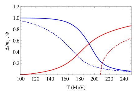
Figure 1: Normalized chiral condensate ${\Delta\over m_{q}}$ (blue lines) and Polyakov-loop $\Phi$ (red lines) as functions of the temperature $T$ for $\mu_{B}=\mu_{I}=0$. See main text for details.

In Fig. 1, we show the normalized chiral condensate ${\Delta\over m_{q}}$ (blue lines) and the expectation value of the Polyakov loop $\Phi$ as functions of the temperature $T$ at $\mu_{B}=\mu_{I}=0$ using the polynomial potential (38). The blue dashed line is the chiral condensate obtained in QM model while the blue solid line is obtained in the PQM model, i.e. with the coupling between the order parameters. Similarly, the red dashed line is obtained using the pure-glue potential for $\Phi$ (with the $N_{f}$ dependent $T_{0}=208\;\text{MeV}$), while the red solid line is obtained in the PQM model. We notice that the critical temperature for the chiral transition moves to the right, i.e. to higher temperatures while the transition temperature for deconfinement moves to the left. They are now within a few MeV of each other, with the deconfinement transition occurring at slightly lower temperature than the chiral transition.

V Phase diagram

In this section, we discuss the phase diagram in the $\mu_{I}$–$T$ plane. In the numerical work below, we set $N_{c}=3$, $m_{\pi}=140$ MeV, and $f_{\pi}=93$ MeV. We vary $m_{\sigma}$ between 500 and 600 MeV.

In Fig. 2, we show the chiral (blue line) and pion condensates (red line) as functions of $\mu_{I}$ at zero temperature. We notice the onset of pion condensation which takes place at exactly $\mu_{I}={1\over 2}m_{\pi}$ as we will discuss in some detail below. Moreover, the quark condensate decreases with $\mu_{I}$ once the pion condensate is nonzero. Finally, all physical quantities, are independent of $\mu_{I}$ from $\mu_{I}=0$ all the way up to $\mu_{I}={1\over 2}m_{\pi}$. For example, the effective potential is independent of $\mu_{I}$, implying via Eq. (5) that the isospin density vanishes. This is an example of the Silver Blaze property cohen and was discussed in detail in the context of pion condensation in Refs. lorenz ; patrick . We refer to this region as the vacuum phase.

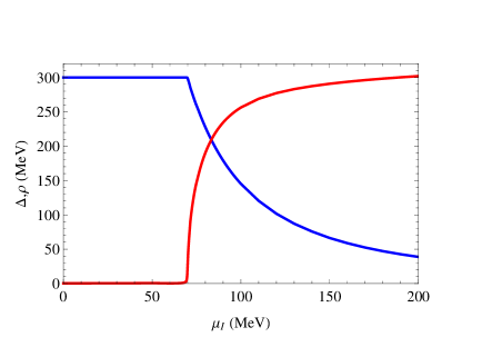
Figure 2: Chiral (blue line) and pion condensates (red line) $\Delta$ and $\rho$ as functions of the isospin chemical potential $\mu_{I}$ at $T=0$.

In Fig. 3, we show the phase diagram in the $\mu_{I}$–$T$ plane for $\mu_{B}=0$ without the Polyakov loop, i.e. for the quark-meson model. The blue line is the transition line for the chiral transition and the green line is the transition line for condensation of $\pi^{+}$, The blue line is defined by the inflection point of the order parameter $\Delta$ as functions of $T$ for fixed $\mu_{I}$. and the black dotted line indicates the crossover from a pion condensate to a BCS state with Cooper pairs.

The onset of pion condensation at $T=0$ is for $\mu_{I}={1\over 2}m_{\pi}$, which is guaranteed by the way we have determined the parameters in the Lagrangian. This was explicitly demonstrated in Ref. patrick . We can understand this result by considering the energy of a zero-momentum pion in the vacuum phase is $m_{\pi}-2\mu_{I}$. If condensations of pions is a second order transition, it must take place exactly at a point where the (medium-dependent) mass of the pion drops to zero, because in the condensed phase there is a massless Nambu-Goldstone mode associated with the breaking of a $U(1)$ symmetry. If one uses matching at tree level, there will be finite corrections to this relation. Likewise, if one uses the effective potential itself to define the pion mass, one uses the pion self-energy at zero external momentum and so the pole of the propagator is not at the physical mass. Again there will be finite corrections and in some cases, the deviation from the exact result can be significant lorenz .

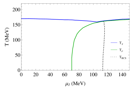
Figure 3: Phase diagram in the $\mu_{I}$–$T$ plane for $\mu_{B}=0$ without Polyakov loop. See main text for details.

The condensation of pions is always a second-order transition with mean-field critical exponents. The order of the transition to a BEC is in agreement with the functional renormalization group application to the QM model in Ref. lorenz . The critical isospin chemical potential is fairly constant for temperatures up to approximately $T=100$ MeV, after which it rapidly increases. For large values of $\mu_{I}$ the critical temperature for pion condensation stays at $T_{\rho}\approx 187$ MeV. We also notice that the chiral transition temperature line $T_{\chi}$ meets the critical temperature line for pion condensation $T_{\rho}$ at $\left(\mu_{I}^{\rm meet},T^{\rm meet}\right)\approx(105,159)$ MeV, and coincide for larger values of $\mu_{I}$.

As we have seen, we enter the BEC phase when $\mu_{I}$ exceeds ${1\over 2}m_{\pi}$. As $\mu_{I}$ increases the quark mass $\Delta$ decreases as shown in Fig. 2. Once $\mu_{I}>\Delta$, the $u$-quark and $\bar{d}$-quark energies, Eqs. (19) and (20), are no longer minimized for ${p}=0$, but for $p=\sqrt{\mu_{I}^{2}-\Delta^{2}}$. This change is a signal of the BEC-BCS crossover. Although the BEC-BCS crossover is not particularly sharp, it is typically defined by the condition $\mu_{I}>\Delta$ sun ; tomas . The crossover starts at $\mu_{I}=113$ MeV for $T=0$ and is almost independent of the temperature, as can be seen from the Figure.

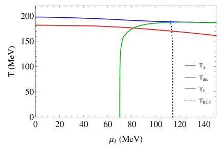
Figure 4: Phase diagram in the $\mu_{I}-T$ plane for $\mu_{B}=0$ with the Polyakov-loop potential Eq. (38). See main text for details.

In Fig. 4, we show the phase diagram in the $\mu_{I}$–$T$ plane at zero baryon chemical potential with the Polyakov loop and ${{\cal U}\over T^{4}}$ given by (38). The green line is the critical line for Bose-Einstein condensation of charged pions, the red line is the critical line for deconfinement, and the blue line is the critical line for the chiral transition. Finally, the black dotted line indicates the BEC-BCS transition line. The blue and red lines are defined by the inflection point of the order parameters $\Delta$ and $\Phi$ as functions of $T$ for fixed $\mu_{I}$. As in the QM model, the transition temperature line $T_{\chi}$ joins the critical temperature for pion condensation at $\left(\mu_{I}^{\rm meet},T^{\rm meet}\right)\approx(116,187)$ MeV. The transition line for deconfinement lies approximately 15 MeV below the chiral transition line for $\mu_{I}=0$ increasing somewhat for large values of $\mu_{I}$.

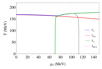
Figure 5: Phase diagram in the $\mu_{I}-T$ plane for $\mu_{B}=0$ with the Polyakov-loop potential Eq. (42). See main text for details.

The gap between the chiral and deconfinement line can be reduced by using a logarithmic Polyakov potential (42) instead of Eq. (38) and decreasing the sigma mass. For $m_{\sigma}=500$ MeV the two lines basically coincide at $T=0$ as seen in Fig. 5. The chiral and deconfinement transition line also meet the pion-condensed line at a point for a smaller value of $\mu_{I}$ as compared to Fig. 4, $\left(\mu_{I}^{\rm meet},T^{\rm meet}\right)\approx(75,164)$ MeV.

For completeness, we show in Fig. 6 the phase diagram in the standard mean-field approximation (sMFA), which is a common approximation used in the literature, where one ignores the loop corrections to the vacuum potential, i.e. uses Eq. (18) instead of Eq. (28). We find the critical temperature for pion condensation to be smaller than for the one-loop potential in Fig. 4. We also find a first-order transition of the pion condensate above a critical isospin chemical potential $\mu_{I}\approx 86$ MeV, indicated by the black dot in the figure. This critical point is absent once we go beyond the sMFA, at least in the region of $\mu_{I}$ considered here.

Figure 6: Phase diagram in the $\mu_{I}-T$ plane for $\mu_{B}=0$ in the standard mean field approximation with the Polyakov-loop potential Eq. (38). See main text for details.

Our phase diagram is in qualitative good agreement with that obtained by Brandt, Endrődi, Schmalzbauer using lattice simulations gergy1 ; gergy2 ; gergy3 , in particular if we use a logarithmic Polyakov loop potential and choose a lower sigma mass of $500$ MeV. We believe that the quantitative differences (essentially the temperature dependence of the various transition lines) can mainly be attributed to the fact that we have two light flavors, while they consider 2+1 flavors; for example the deconfinement transition temperature decreases with the number of quarks and our transition line is consistently higher. They find that chiral and BEC transition lines meet at a triple point, beyond which they coincide. The latter transition is again found to be second order for all values of $\mu_{I}$ and the scaling analysis is consistent with the $O(2)$ universality class. They computed contour lines of the expectation values of the renormalized Polyakov loop $\Phi$ for values 0.2, 0.4, 0.6, 0.8, and 1.0. Given their renormalization prescription for the Polyakov loop, developed in renpol , a possible choice for $T_{\rm dec}$ is $\Phi=1$, which implies that it coincides with $T_{\chi}$ within errors gergy3 . Finally, we mention that the deconfinement line penetrates smoothly into the BEC phase and that they identify this line with the BEC-BCS transition.

Appendix A Integrals

With dimensional regularization, the momentum integral is generalized to $d=3-2\epsilon$ spatial dimensions. We define the dimensionally regularized integral by

$$\int_{p} = \left({e^{\gamma_{E}}\Lambda^{2}\over 4\pi}\right)^{\epsilon}\int{d^{d}p\over(2\pi)^{d}}\;,$$ (48)

where $\Lambda$ is the renormalization scale in the modified minimal subtraction scheme $\overline{\rm MS}$. In order to calculate the vacuum part of the effective potential, we need the vacuum integrals

$$\int_{p}\sqrt{p^{2}+M^{2}} = -{M^{4}\over(4\pi)^{2}}\left({e^{\gamma_{E}}\Lambda^{2}\over M^{2}}\right)^{\epsilon}\Gamma(-2+\epsilon)=-{M^{4}\over 2(4\pi)^{2}}\left({\Lambda^{2}\over M^{2}}\right)^{\epsilon}\left[{1\over\epsilon}+{3\over 2}+{\cal O}(\epsilon)\right]\;,$$ (49)

$$\int_{p}{1\over(p^{2}+M^{2})^{3\over 2}} = {4\over(4\pi)^{2}}\left({e^{\gamma_{E}}\Lambda^{2}\over M^{2}}\right)^{\epsilon}\Gamma(\epsilon)={4\over(4\pi)^{2}}\left({\Lambda^{2}\over M^{2}}\right)^{\epsilon}\left[{1\over\epsilon}+{\cal O}(\epsilon)\right]\;.$$ (50)

Appendix B Parameter fixing

In this Appendix, we briefly discuss the fixing of the model parameters. At tree level, the relations between these parameters and the physical quantities are given by Eqs. (16)–(17). In the on-shell scheme, the counterterms are chosen such that they exactly cancel the loop corrections to the self-energies and couplings evaluated on the mass shell, and such that the residues evaluated on shell are unity. Consequently, the renormalized parameters are independent of the renormalization scale and satisfy the tree-level relations sir1 ; sir2 ; hollik . In the $\overline{\rm MS}$ scheme, the counterterms are chosen so that they cancel only the poles in $\epsilon$ of the loop corrections. The bare parameters are the same in the two schemes, which means that we can relate the corresponding renormalized parameters. The running parameters in the $\overline{\rm MS}$ scheme can therefore be expressed in terms of the physical masses $m_{\sigma}$, $m_{\pi}$, and $m_{q}$ as well as the pion decay constant $f_{\pi}$. In Ref. crew we found

$$m^{2}_{\overline{\text{\tiny MS}}} = m^{2}+8ig^{2}N_{c}\left[A(m_{q}^{2})+\mbox{$1\over 4$}(m_{\sigma}^{2}-4m_{q}^{2})B(m_{\sigma}^{2})-\mbox{$3\over 4$}m_{\pi}^{2}B(m_{\pi}^{2})\right]-\delta m^{2}_{\overline{\text{\tiny MS}}}$$ (51)

$$= m^{2}+\dfrac{4g^{2}N_{c}}{(4\pi)^{2}}\left[m^{2}\log\mbox{$\Lambda^{2}\over m_{q}^{2}$}-2m_{q}^{2}-{1\over 2}\left(m_{\sigma}^{2}-4m_{q}^{2}\right)F(m_{\sigma}^{2})+{3\over 2}{m_{\pi}^{2}}F(m_{\pi}^{2})\right]\;,$$

$$\lambda_{\overline{\text{\tiny MS}}} = \lambda-\dfrac{12ig^{2}N_{c}}{f_{\pi}^{2}}(m_{\sigma}^{2}-4m_{q}^{2})B(m_{\sigma}^{2})+\dfrac{12ig^{2}N_{c}}{f_{\pi}^{2}}m_{\pi}^{2}B(m_{\pi}^{2})-4i\lambda g^{2}N_{c}\left[B(m_{\pi}^{2})+m_{\pi}^{2}B^{\prime}(m_{\pi}^{2})\right]-\delta\lambda_{\overline{\text{\tiny MS}}}$$ (52)

$$= \lambda+\bigg{\{}\dfrac{12g^{2}N_{c}}{(4\pi)^{2}f_{\pi}^{2}}\left[(m_{\sigma}^{2}-4m_{q}^{2})\left(\log\mbox{$\Lambda^{2}\over m_{q}^{2}$}+F(m_{\sigma}^{2})\right)+m_{\sigma}^{2}\left(\log\mbox{$\Lambda^{2}\over m_{q}^{2}$}+F(m_{\pi}^{2})+m_{\pi}^{2}F^{\prime}(m_{\pi}^{2})\right)\right.$$

$$\left.-m_{\pi}^{2}\left(2\log\mbox{$\Lambda^{2}\over m_{q}^{2}$}+2F(m_{\pi}^{2})+F^{\prime}(m_{\pi}^{2})\right)\right]\bigg{\}}\;,$$

$$g_{\overline{\text{\tiny MS}}}^{2} = g^{2}-4ig^{4}N_{c}\left[B(m_{\pi}^{2})+m_{\pi}^{2}B^{\prime}(m_{\pi}^{2})\right]-\delta g_{\overline{\text{\tiny MS}}}^{2}={m_{q}^{2}\over f_{\pi}^{2}}\left\{1+\dfrac{4g^{2}N_{c}}{(4\pi)^{2}}\left[\log\mbox{$\Lambda^{2}\over m_{q}^{2}$}+F(m_{\pi}^{2})+m_{\pi}^{2}F^{\prime}(m_{\pi}^{2})\right]\right\}\;,$$ (53)

$$h_{\overline{\text{\tiny MS}}} = h-2ig^{2}N_{c}m_{\pi}^{2}f_{\pi}\left[B(m_{\pi}^{2})-m_{\pi}^{2}B^{\prime}(m_{\pi}^{2})\right]-\delta h_{\overline{\text{\tiny MS}}}=h\left\{1+{2g^{2}N_{c}\over(4\pi)^{2}}\left[\log\mbox{$\Lambda^{2}\over m_{q}^{2}$}+F(m_{\pi}^{2})-m_{\pi}^{2}F^{\prime}(m_{\pi}^{2})\right]\right\}\;,$$ (54)

where $A(m_{q}^{2})$, $B(p^{2})$, and $B^{\prime}(p^{2})$ are integrals in $d=4-2\epsilon$ dimensions in Minkowski space. Going to Euclidean space, they can be straightforwardly computed and read

$$A(m^{2}_{q}) = \int_{k}{1\over k^{2}-m^{2}_{q}}$$ (55)

$$= {im^{2}_{q}\over(4\pi)^{2}}\left({\Lambda^{2}\over m_{q}^{2}}\right)\left[{1\over\epsilon}+1+{\cal O}(\epsilon)\right]\;,$$

$$B(p^{2}) = \int_{k}{1\over(k^{2}-m_{q}^{2})[(k+p)^{2}-m_{q}^{2}]}$$ (56)

$$= {i\over(4\pi)^{2}}\left({\Lambda^{2}\over m_{q}^{2}}\right)\left[{1\over\epsilon}+F(p^{2})+{\cal O}(\epsilon)\right]\;,$$

$$B^{\prime}(p^{2}) = {i\over(4\pi)^{2}}F^{\prime}(p^{2})\;,$$ (57)

where we have defined

$$F(p^{2}) = 2-2r\arctan\left({1\over r}\right)\;,$$ (58)

$$F^{\prime}(p^{2}) = {4m_{q}^{2}r\over p^{2}(4m_{q}^{2}-r^{2})}\arctan\left({1\over r}\right)-{1\over p^{2}}\;,$$ (59)

with $r=\sqrt{{4m_{q}^{2}\over p^{2}}-1}$.

The running parameters satisfy the following renormalization group equations

$$\Lambda{dm_{\overline{\text{\tiny MS}}}^{2}(\Lambda)\over d\Lambda} = {8N_{c}m^{2}_{\overline{\text{\tiny MS}}}(\Lambda)g_{\overline{\text{\tiny MS}}}^{2}(\Lambda)\over(4\pi)^{2}}\;,$$ (60)

$$\Lambda{dg_{\overline{\text{\tiny MS}}}^{2}(\Lambda)\over d\Lambda} = {8N_{c}g_{\overline{\text{\tiny MS}}}^{4}(\Lambda)\over(4\pi)^{2}}\;,$$ (61)

$$\Lambda{d\lambda_{\overline{\text{\tiny MS}}}(\Lambda)\over d\Lambda} = {16N_{c}\over(4\pi)^{2}}\left[\lambda_{\overline{\text{\tiny MS}}}(\Lambda)g^{2}_{\overline{\text{\tiny MS}}}(\Lambda)-6g^{4}_{\overline{\text{\tiny MS}}}(\Lambda)\right]\;,$$ (62)

$$\Lambda{dh_{\overline{\text{\tiny MS}}}(\Lambda)\over d\Lambda} = {4N_{c}g^{2}_{\overline{\text{\tiny MS}}}(\Lambda)h_{\overline{\text{\tiny MS}}}(\Lambda)\over(4\pi)^{2}}\;.$$ (63)

The solutions to Eqs. (60)–(63) are

$$m_{\overline{\text{\tiny MS}}}^{2}(\Lambda) = {m_{0}^{2}\over 1-{4g_{0}^{2}N_{c}\over(4\pi)^{2}}\log{\Lambda^{2}\over\Lambda_{0}^{2}}}\;.$$ (64)

$$g_{\overline{\text{\tiny MS}}}^{2}(\Lambda) = {g_{0}^{2}\over 1-{4g_{0}^{2}N_{c}\over(4\pi)^{2}}\log{\Lambda^{2}\over\Lambda_{0}^{2}}}\;,$$ (65)

$$\lambda_{\overline{\text{\tiny MS}}}(\Lambda) = {\lambda_{0}-{48g_{0}^{4}N_{c}\over(4\pi)^{2}}\log{\Lambda^{2}\over\Lambda_{0}^{2}}\over\left(1-{4g_{0}^{2}N_{c}\over(4\pi)^{2}}\log{\Lambda^{2}\over\Lambda_{0}^{2}}\right)^{2}}\;,$$ (66)

$$h_{\overline{\text{\tiny MS}}}(\Lambda) = {h_{0}\over 1-{2g_{0}^{2}N_{c}\over(4\pi)^{2}}\log{\Lambda^{2}\over\Lambda_{0}^{2}}}\;,$$ (67)

where $m_{0}^{2}$, $g_{0}^{2}$, $\lambda_{0}$ and $h_{0}$, are the values of the running parameters at the scale $\Lambda_{0}$. We choose $\Lambda_{0}$ to satisfy

$$\log{\Lambda_{0}^{2}\over m_{q}^{2}}+F(m_{\pi}^{2})+m_{\pi}^{2}F^{\prime}(m_{\pi}^{2}) = 0\;.$$ (68)

One can now evaluate Eqs. (51)–(54) at the scale $\Lambda=\Lambda_{0}$ to find $m_{0}^{2}$, $\lambda_{0}$, $g_{0}^{2}$, and $h_{0}$. Inserting Eqs. (64)–(67) into Eq. (27) using the results for $m_{0}^{2}$, $\lambda_{0}$, $g_{0}^{2}$, and $h_{0}$, we obtain the final result Eq. (28).

References

(1)
K. Rajagopal and F. Wilczek,
At the frontier of particle physics, Vol. 3
(World Scientific, Singapore, p 2061) (2001).
(2)
M. G. Alford, A. Schmitt, K. Rajagopal, and T. Schäfer,
Rev. Mod. Phys. 80, 1455 (2008).
(3)
K. Fukushima and T. Hatsuda,
Rept. Prog. Phys. 74, 014001 (2011).
(4)
Y. Aoki, Z. Fodor, S. Katz, and K. Szabo,
Phys. Lett. B 643, 46 (2006).
(5)
Y. Aoki, S. Borsanyi, S. Dürr, Z. Fodor, S.D. Katz et al.,
JHEP 09 06, 088 (2009),
(6)
S. Borsanyi et al. (Wuppertal-Budapest Collaboration),
JHEP 10 09, 073 (2010).
(7)
A. Bazavov, T. Bhattacharya, M. Cheng, C. DeTar, H. Ding et al.,
Phys. Rev. D 85, 054503 (2012).
(8) J. B. Kogut, M. A. Stephanov, D. Toublan, and J. J. M. Verbaarschot,
Nucl. Phys. B 582, 477 (2000).
(9) J. B. Kogut (Illinois U., Urbana), M. A. Stephanov, and D. Toublan,
Phys. Lett. B 464, 183 (1999).
(10)
D. T. Son and M. A. Stephanov,
Phys. Rev. Lett. 86, 592 (2001).
(11) G. S. Bali, F. Bruckmann, G. Endrődi, Z. Fodor, S. D. Katz , S. Krieg,
A. Schafer, and K. K. Szabo,
JHEP 12 02, 044 (2012).
(12) D. Kharzeev, K. Landsteiner, A. Schmitt, and H.-U. Yee (ed)
Lect. Notes Phys. 871, 1 (2013).
(13)
J. O. Andersen, W. R. Naylor, A. Tranberg,
Rev. Mod. Phys. 88, 025001 (2016).
(14)
J. B. Kogut and D. K. Sinclair,
Phys. Rev. D 66, 014508 (2002).
(15)
J. B. Kogut and D. K. Sinclair,
Phys. Rev D 66 034505 (2002).
(16) B. B. Brandt and G. Endrődi,
PoS LATTICE 2016, 039 (2016).
(17) B. B. Brandt, G. Endrődi,, and S. Schmalzbauer,
EPJ Web Conf. 175, 07020 (2018).
(18) B. B. Brandt, G. Endrődi, and S. Schmalzbauer,
Phys. Rev. D 97, 054514 (2018).
(19)
K. Splittorff, D. T. Son, M. A. Stephanov,
Phys. Rev. D 64, 016003 (2001).
(20)
M. Loewe and C. Villavicencio,
Phys. Rev. D 67, 074034 (2003).
(21)
E. S. Fraga, L. F. Palhares and C. Villavicencio,
Phys. Rev. D 79, 014021 (2009).
(22)
S. Carignano, L. Lepori, A. Mammarella, M. Mannarelli and G. Pagliaroli,
Eur. Phys. J. A 53, 35 (2017).
(23)
D. Toublan and J. B. Kogut,
Phys. Lett. B 605, 129 (2005).
(24)
B. Klein, D. Toublan and J. J. M. Verbaarschot,
Phys. Rev. D 68, 014009 (2003).
(25)
M. Frank, M. Buballa, and M. Oertel,
Phys. Lett. B 562, 221 (2003).
(26)
D. Toublan, and J. B. Kogut, Phys. Lett. B 564, 212 (2003).
(27)
A. Barducci, R. Casalbuoni, G. Pettini, and L. Ravagli
Phys. Rev. D 69, 096004 (2004).
(28)
L. He, and P.-F. Zhuang,
Phys. Lett. B 615, 93 (2005).
(29)
L. He, M. Jin and P.-F. Zhuang,
Phys. Rev. D 71, 116001, (2005).
(30) L. He, M. Jin, and P.-F. Zhuang,
Phys. Rev. D 74, 036005 (2006).
(31) D. Ebert and K. G. Klimenko,
J. Phys. G 32, 599 (2006).
(32) D. Ebert and K. G. Klimenko,
Eur. Phys. J. C 46, 771 (2006).
(33)
G.-F. Sun, L. He, and P.-F. Zhuang,
Phys. Rev. D 75, 096004 (2007).
(34) J. O. Andersen and L. Kyllingstad,
J. Phys. G 37, 015003 (2009).
(35)
H. Abuki, R. Anglani, R. Gatto, M. Pellicoro, and M. Ruggieri,
Phys. Rev. D 79, 034032 (2009).
(36)
C.-F. Mu, L. He, and Y. Liu, Phys. Rev. D 82, 056006 (2010).
(37)
T. Xia, L. He and P. Zhuang,
Phys. Rev. D 88, 056013 (2013).
(38)
K. Kamikado, N. Strodthoff, L. von Smekal, and J. Wambach
Phys. Lett. B 718, 1044 (2013).
(39)
H. Ueda, T. Z. Nakano, A. Ohnishi, M. Ruggieri, and K. Sumiyoshi,
Phys. Rev. D 88, 074006 (2013).
(40)
R. Stiele, E. S. Fraga and J. Schaffner-Bielich,
Phys. Lett. B 729, 72 (2014).
(41)
J. O. Andersen and P. Kneschke, Phys. Rev. D 97, 076005 (2018).
(42)
T. D. Cohen and S. Sen, Nucl. Phys. A 942, 39 (2015).
(43)
L. G. Yaffe and B. Svetitsky,
Phys. Rev. D 26,963 (1982).
(44)
B. Svetitsky and L. G. Yaffe,
Nucl. Phys. B 210, 423 (1982).
(45)
C. Ratti, M. A. Thaler, and W. Weise, Phys. Rev. D 73, 014019 (2006).
(46)
S. Roessner, C. Ratti and W. Weise, Phys. Rev. D 75, 034007 (2007).
(47)
B.-J. Schaefer, J. M. Pawlowski, and J. Wambach,
Phys. Rev. D 76, 074023 (2007).
(48)
K. Fukushima, Phys. Rev. D 77, 114028. (2008).
(49)
Karsch, F., E. Laermann, and A. Peikert,
Nucl. Phys. B 605, 579 (2001).
(50)
T. D. Cohen, Phys. Rev. Lett. 91, 222001 (2003).
(51)
T. Brauner, K. Fukushima, and Y. Hidaka,
Phys. Rev. D 80, 074035 (2009); ibid D 81, 119904 (2010).
(52)
S. Borsanyi et al,
JHEP 12 08, 126 (2012).
(53)
P. Adhikari, J. O. Andersen, and P. Kneschke,
Phys. Rev. D 96, 016013 (2017).
(54)
A. Sirlin, Phys. Rev. D 22, 971 (1980).
(55)
A. Sirlin, Phys. Rev. D 29, 89 (1984).
(56)
M. Bohm, H. Spiesberger, and W. Hollik, Fortsch. Phys. 34, 687 (1986).