Flavour Dynamics and Violations of the CP Symmetry

Abstract

An overview of flavour physics and ${\cal CP}$-violating phenomena is presented. The Standard Model quark-mixing mechanism is discussed in detail and its many successful experimental tests are summarized. Flavour-changing transitions put very stringent constraints on new-physics scenarios beyond the Standard Model framework. Special attention is given to the empirical evidences of ${\cal CP}$ violation and their important role in our understanding of flavour dynamics. The current status of the so-called flavour anomalies is also reviewed.

1 Fermion families

We have learnt experimentally that there are six different quark flavours; three of them, $u\,$, $c\,$, $t\,$, with electric charge $Q=+\frac{2}{3}$ (up-type), and the other three, $d\,$, $s\,$, $b\,$, with $Q=-\frac{1}{3}$ (down-type). There are also three different charged leptons, $e\,$, $\mu\,$, $\tau$, with $Q=-1$ and their corresponding neutrinos, $\nu_{e}\,$, $\nu_{\mu}\,$, $\nu_{\tau}\,$, with $Q=0$. We can include all these particles into the $SU(3)_{C}\otimes SU(2)_{L}\otimes U(1)_{Y}$ Standard Model (SM) framework [1, 2, 3], by organizing them into three families of quarks and leptons:

$$\left[\begin{array}[]{cc}\nu_{e}&u\\ e^{-}&d\hskip 0.7pt^{\prime}\end{array}\right]\,,\qquad\quad\left[\begin{array}[]{cc}\nu_{\mu}&c\\ \mu^{-}&s\hskip 0.7pt^{\prime}\end{array}\right]\,,\qquad\quad\left[\begin{array}[]{cc}\nu_{\tau}&t\\ \tau^{-}&b\hskip 0.6pt^{\prime}\end{array}\right]\,,$$ (1)

where (each quark appears in three different colours)

$$\left[\begin{array}[]{cc}\nu_{i}&u_{i}\\ \ell^{-}_{i}&d\hskip 0.7pt^{\prime}_{i}\end{array}\right]\quad\equiv\quad\left(\begin{array}[]{c}\nu_{i}\\ \ell^{-}_{i}\end{array}\right)_{L}\,,\quad\left(\begin{array}[]{c}u_{i}\\ d\hskip 0.7pt^{\prime}_{i}\end{array}\right)_{L}\,,\quad\ell^{-}_{iR}\;,\quad u^{\phantom{j}}_{iR}\;,\quad d\hskip 0.7pt^{\prime}_{iR}\;,$$ (2)

plus the corresponding antiparticles. Thus, the left-handed fields are $SU(2)_{L}$ doublets, while their right-handed partners transform as $SU(2)_{L}$ singlets. The three fermionic families appear to have identical properties (gauge interactions); they differ only by their mass and their flavour quantum numbers.

The fermionic couplings of the photon and the $Z$ boson are flavour conserving, the neutral gauge bosons couple to a fermion and its corresponding antifermion. In contrast, the $W^{\pm}$ bosons couple any up-type quark with all down-type quarks because the weak doublet partner of $u_{i}$ turns out to be a quantum superposition of down-type mass eigenstates: $d\hskip 0.7pt^{\prime}_{i}=\sum_{j}\mathbf{V}_{ij}\,d^{\phantom{j}}_{j}$. This flavour mixing generates a rich variety of observable phenomena, including ${\cal CP}$-violation effects, which can be described in a very successful way within the SM [4, 5].

In spite of its enormous phenomenological success, The SM does not provide any real understanding of flavour. We do not know yet why fermions are replicated in three (and only three) nearly identical copies. Why the pattern of masses and mixings is what it is? Are the masses the only difference among the three families? What is the origin of the SM flavour structure? Which dynamics is responsible for the observed ${\cal CP}$ violation? The fermionic flavour is the main source of arbitrary free parameters in the SM: 9 fermion masses, 3 mixing angles and 1 complex phase, for massless neutrinos. 7 (9) additional parameters arise with non-zero Dirac (Majorana) neutrino masses: 3 masses, 3 mixing angles and 1 (3) phases. The problem of fermion mass generation is deeply related with the mechanism responsible for the electroweak Spontaneous Symmetry Breaking (SSB). Thus, the origin of these parameters lies in the most obscure part of the SM Lagrangian: the scalar sector. Clearly, the dynamics of flavour appears to be “terra incognita” which deserves a careful investigation.

The following sections contain a short overview of the quark flavour sector and its present phenomenological status. The most relevant experimental tests are briefly described. A more pedagogic introduction to the SM can be found in Ref. [4].

2 Flavour structure of the Standard Model

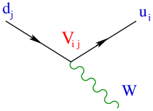
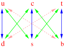
Figure 1: Flavour-changing transitions through the charged-current couplings of the $W^{\pm}$ bosons.

In the SM flavour-changing transitions occur only in the charged-current sector (Fig. 1):

$${\cal L}_{\rm\scriptstyle CC}\,=\,-{g\over 2\sqrt{2}}\,\left\{W^{\dagger}_{\mu}\,\left[\,\sum_{ij}\;\bar{u}_{i}\,\gamma^{\mu}(1-\gamma_{5})\,\mathbf{V}_{\!ij}\,d_{j}\;+\;\sum_{\ell}\;\bar{\nu}_{\ell}\,\gamma^{\mu}(1-\gamma_{5})\,\ell\,\right]\,+\,\mathrm{h.c.}\right\}\,.$$ (3)

The so-called Cabibbo–Kobayashi–Maskawa (CKM) matrix $\mathbf{V}$ [6, 7] is generated by the same Yukawa couplings giving rise to the quark masses. Before SSB, there is no mixing among the different quarks, $\mathbf{V}=\mathbf{I}$. In order to understand the origin of the matrix $\mathbf{V}$ , let us consider the general case of $N_{G}$ generations of fermions, and denote $\nu\hskip 0.7pt^{\prime}_{j}$, $\ell\hskip 0.7pt^{\prime}_{j}$, $u\hskip 0.6pt^{\prime}_{j}$, $d\hskip 0.7pt^{\prime}_{j}$ the members of the weak family $j$  ($j=1,\ldots,N_{G}$), with definite transformation properties under the gauge group. Owing to the fermion replication, a large variety of fermion-scalar couplings are allowed by the gauge symmetry. The most general Yukawa Lagrangian has the form

$${\cal L}_{Y} = -\,\sum_{jk}\;\left\{\left(\bar{u}\hskip 0.6pt^{\prime}_{j},\bar{d}\hskip 0.7pt^{\prime}_{j}\right)_{L}\left[\,c^{(d)}_{jk}\,\left(\begin{array}[]{c}\phi^{(+)}\\ \phi^{(0)}\end{array}\right)\,d\hskip 0.7pt^{\prime}_{kR}\;+\;c^{(u)}_{jk}\,\left(\begin{array}[]{c}\phi^{(0)*}\\ -\phi^{(-)}\end{array}\right)\,u\hskip 0.6pt^{\prime}_{kR}\,\right]\right.$$ (11)

$$\qquad\quad\left.+\;\;\left(\bar{\nu}\hskip 0.7pt^{\prime}_{j},\bar{\ell}\hskip 0.7pt^{\prime}_{j}\right)_{L}\,c^{(\ell)}_{jk}\,\left(\begin{array}[]{c}\phi^{(+)}\\ \phi^{(0)}\end{array}\right)\,\ell\hskip 0.7pt^{\prime}_{kR}\,\right\}\;+\;\mathrm{h.c.},$$

where $\phi^{T}(x)\,\equiv\,\left(\phi^{(+)},\phi^{(0)}\right)$ is the SM scalar doublet and $c^{(d)}_{jk}$, $c^{(u)}_{jk}$ and $c^{(\ell)}_{jk}$ are arbitrary coupling constants. The second term involves the charge-conjugate scalar field $\phi^{c}(x)=i\,\sigma_{2}\,\phi^{*}(x)$.

In the unitary gauge $\phi^{T}(x)\,\equiv\,\frac{1}{\sqrt{2}}\,\left(0,v+H(x)\right)$, where $v$ is the electroweak vacuum expectation value and $H(x)$ the Higgs field. The Yukawa Lagrangian can then be written as

$${\cal L}_{Y}\,=\,-\left(1+{H\over v}\right)\,\left\{\,\overline{\mathbf{d}}\hskip 0.6pt^{\prime}_{L}\,\mathbf{M}_{d}^{\prime}\,\mathbf{d}\hskip 0.6pt^{\prime}_{R}\;+\;\overline{\mathbf{u}}\hskip 0.6pt^{\prime}_{L}\,\mathbf{M}_{u}^{\prime}\,\mathbf{u}\hskip 0.6pt^{\prime}_{R}\;+\;\overline{\boldsymbol{\ell}}\hskip 0.2pt^{\prime}_{L}\,\mathbf{M}^{\prime}_{\ell}\,\boldsymbol{\ell}\hskip 0.2pt^{\prime}_{R}\;+\;\mathrm{h.c.}\right\}.$$ (12)

Here, $\mathbf{d}\hskip 0.6pt^{\prime}$, $\mathbf{u}\hskip 0.6pt^{\prime}$ and $\boldsymbol{\ell}\hskip 0.2pt^{\prime}$ denote vectors in the $N_{G}$-dimensional flavour space, with components $d\hskip 0.7pt^{\prime}_{j}$, $u\hskip 0.6pt^{\prime}_{j}$ and $\ell\hskip 0.7pt^{\prime}_{j}$, respectively, and the corresponding mass matrices are given by

$$(\mathbf{M}^{\prime}_{d})_{ij}\,\equiv\,c^{(d)}_{ij}\,{v\over\sqrt{2}}\,,\qquad(\mathbf{M}^{\prime}_{u})_{ij}\,\equiv\,c^{(u)}_{ij}\,{v\over\sqrt{2}}\,,\qquad(\mathbf{M}^{\prime}_{\ell})_{ij}\,\equiv\,c^{(\ell)}_{ij}\,{v\over\sqrt{2}}\,.$$ (13)

The diagonalization of these mass matrices determines the mass eigenstates $d_{j}$, $u_{j}$ and $\ell_{j}$, which are linear combinations of the corresponding weak eigenstates $d\hskip 0.7pt^{\prime}_{j}$, $u\hskip 0.6pt^{\prime}_{j}$ and $\ell\hskip 0.7pt^{\prime}_{j}$, respectively.

The matrix $\mathbf{M}_{d}^{\prime}$ can be decomposed as $\mathbf{M}_{d}^{\prime}=\mathbf{H}_{d}\,\mathbf{U}_{d}=\mathbf{S}_{d}^{\dagger}\,\mathbf{{\cal M}}_{d}\,\mathbf{S}_{d}\,\mathbf{U}_{d}$, where  $\mathbf{H}_{d}\equiv\sqrt{\mathbf{M}_{d}^{\prime}\mathbf{M}_{d}^{\prime\dagger}}$ is an Hermitian positive-definite matrix, while $\mathbf{U}_{d}$ is unitary. $\mathbf{H}_{d}$ can be diagonalized by a unitary matrix $\mathbf{S}_{d}$; the resulting matrix $\mathbf{{\cal M}}_{d}$ is diagonal, Hermitian and positive definite. Similarly, one has  $\mathbf{M}_{u}^{\prime}=\mathbf{H}_{u}\,\mathbf{U}_{u}=\mathbf{S}_{u}^{\dagger}\,\mathbf{{\cal M}}_{u}\,\mathbf{S}_{u}\,\mathbf{U}_{u}$  and  $\mathbf{M}_{\ell}^{\prime}=\mathbf{H}_{\ell}\,\mathbf{U}_{\ell}=\mathbf{S}_{\ell}^{\dagger}\,\mathbf{{\cal M}}_{\ell}\,\mathbf{S}_{\ell}\,\mathbf{U}_{\ell}$. In terms of the diagonal mass matrices

$$\mathbf{{\cal M}}_{d}=\mathrm{diag}(m_{d},m_{s},m_{b},\ldots)\,,\quad\;\mathbf{{\cal M}}_{u}=\mathrm{diag}(m_{u},m_{c},m_{t},\ldots)\,,\quad\;\mathbf{{\cal M}}_{\ell}=\mathrm{diag}(m_{e},m_{\mu},m_{\tau},\ldots)\,,$$ (14)

the Yukawa Lagrangian takes the simpler form

$${\cal L}_{Y}\,=\,-\left(1+{H\over v}\right)\,\left\{\,\overline{\mathbf{d}}\,\mathbf{{\cal M}}_{d}\,\mathbf{d}\;+\;\overline{\mathbf{u}}\,\mathbf{{\cal M}}_{u}\,\mathbf{u}\;+\;\overline{\boldsymbol{\ell}}\,\mathbf{{\cal M}}_{\ell}\,\boldsymbol{\ell}\,\right\}\,,$$ (15)

where the mass eigenstates are defined by

$$\mathbf{d}_{L} \!\!\equiv \!\!\mathbf{S}_{d}\,\mathbf{d}\hskip 0.6pt^{\prime}_{L}\,,\qquad\qquad\hskip 15.4pt\mathbf{u}_{L}\>\equiv\;\mathbf{S}_{u}\,\mathbf{u}\hskip 0.6pt^{\prime}_{L}\,,\qquad\qquad\,\,\,\,\,\,\,\,\,\boldsymbol{\ell}_{L}\>\equiv\;\mathbf{S}_{\ell}\,\boldsymbol{\ell}\hskip 0.2pt^{\prime}_{L}\,,$$

$$\mathbf{d}_{R} \!\!\equiv \!\!\mathbf{S}_{d}\mathbf{U}_{d}\,\mathbf{d}\hskip 0.6pt^{\prime}_{R}\,,\qquad\qquad\mathbf{u}_{R}\>\equiv\;\mathbf{S}_{u}\mathbf{U}_{u}\,\mathbf{u}\hskip 0.6pt^{\prime}_{R}\,,\qquad\qquad\boldsymbol{\ell}_{R}\>\equiv\;\mathbf{S}_{\ell}\mathbf{U}_{\ell}\,\boldsymbol{\ell}\hskip 0.2pt^{\prime}_{R}\,.$$ (16)

Note, that the Higgs couplings are flavour-conserving and proportional to the corresponding fermion masses.

Since,  $\overline{\mathbf{f}}\hskip 0.7pt^{\prime}_{L}\,\mathbf{f}\hskip 0.7pt^{\prime}_{L}=\overline{\mathbf{f}}_{L}\,\mathbf{f}_{L}$  and  $\overline{\mathbf{f}}\hskip 0.7pt^{\prime}_{R}\,\mathbf{f}\hskip 0.7pt^{\prime}_{R}=\overline{\mathbf{f}}_{R}\,\mathbf{f}_{R}$  ($f=d,u,\ell$), the form of the neutral-current part of the $SU(3)_{C}\otimes SU(2)_{L}\otimes U(1)_{Y}$ Lagrangian does not change when expressed in terms of mass eigenstates. Therefore, there are no flavour-changing neutral currents (FCNCs) in the SM. This is a consequence of treating all equal-charge fermions on the same footing (GIM mechanism [8]), and guarantees that weak transitions such as $B_{s,d}^{0}\to\ell^{+}\ell^{-}$, $K^{0}\to\mu^{+}\mu^{-}$ or $K^{0}$–$\bar{K}^{0}$ mixing (Fig. 2), which are known experimentally to be very suppressed, cannot happen at tree level. The absence of FCNCs is crucial for the phenomenological success of the SM. However, $\overline{\mathbf{u}}\hskip 0.7pt^{\prime}_{L}\,\mathbf{d}\hskip 0.7pt^{\prime}_{L}=\overline{\mathbf{u}}_{L}\,\mathbf{S}_{u}\,\mathbf{S}_{d}^{\dagger}\,\mathbf{d}_{L}\equiv\overline{\mathbf{u}}_{L}\mathbf{V}\,\mathbf{d}_{L}$. In general, $\mathbf{S}_{u}\not=\mathbf{S}_{d}\,$; thus, if one writes the weak eigenstates in terms of mass eigenstates, a $N_{G}\times N_{G}$ unitary mixing matrix $\mathbf{V}$ appears in the quark charged-current sector as indicated in Eq. (3).

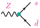
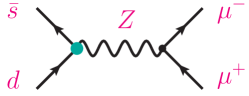
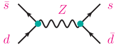
Figure 2: Tree-level FCNC couplings (green solid vertices) are absent in the SM. Therefore, very suppressed (experimentally) transitions such as  $K^{0}\to\mu^{+}\mu^{-}$ or  $K^{0}$–$\bar{K}^{0}$  mixing cannot occur through tree-level exchange.

If neutrinos are assumed to be massless, we can always redefine the neutrino flavours, in such a way as to eliminate the mixing in the lepton sector: $\overline{\mbox{\boldmath$\nu$}}\hskip 0.7pt^{\prime}_{L}\,\boldsymbol{\ell}\hskip 0.7pt^{\prime}_{L}=\overline{\mbox{\boldmath$\nu$}}\hskip 0.7pt_{L}^{\prime}\,\mathbf{S}^{\dagger}_{\ell}\,\boldsymbol{\ell}_{L}\equiv\overline{\mbox{\boldmath$\nu$}}_{L}\,\boldsymbol{\ell}_{L}$. Thus, we have lepton-flavour conservation in the minimal SM without right-handed neutrinos. If sterile $\nu_{R}$ fields are included in the model, one has an additional Yukawa term in Eq. (11), giving rise to a neutrino mass matrix  $(\mathbf{M}^{\prime}_{\nu})_{ij}\equiv c^{(\nu)}_{ij}\,{v/\sqrt{2}}\,$. Thus, the model can accommodate non-zero neutrino masses and lepton-flavour violation through a lepton mixing matrix $\mathbf{V}_{\!L}$ analogous to the one present in the quark sector. Note, however, that the total lepton number  $\mathrm{L}\equiv\mathrm{L}_{e}+\mathrm{L}_{\mu}+\mathrm{L}_{\tau}$  is still conserved. We know experimentally that neutrino masses are tiny and, as shown in Table 1, there are strong bounds on lepton-flavour violating decays. However, we do have a clear evidence of neutrino oscillation phenomena [9]. Moreover, since right-handed neutrinos are singlets under $SU(3)_{C}\otimes SU(2)_{L}\otimes U(1)_{Y}$, the SM gauge symmetry group allows for a right-handed Majorana neutrino mass term, violating lepton number by two units. Non-zero neutrino masses clearly imply interesting new phenomena [4].

Table 1: Best published limits on lepton-flavour-violating transitions [9].

$\rm{Br}(\mu^{-}\to X^{-})\cdot 10^{12}\qquad\quad(90\%\;\mathrm{CL})$
$e^{-}\gamma$	$0.42$	$e^{-}2\gamma$	$72$	$e^{-}e^{-}e^{+}$	$\phantom{1}1.0$
$\Gamma(\mu^{-}+N\to e^{-}+N)/\Gamma(\mu^{-}+N\to\mathrm{capture})\cdot 10^{12}\qquad\quad(90\%\;\mathrm{CL})$
Au	$0.7$	Ti	$4.3$	Pb	46
$\rm{Br}(\tau^{-}\to X^{-})\cdot 10^{8}\qquad\quad(90\%\;\mathrm{CL})$
$e^{-}\gamma$	$3.3$	$e^{-}e^{+}e^{-}$	$\phantom{1}2.7$	$e^{-}\mu^{+}\mu^{-}$	$2.7$	$e^{-}e^{-}\mu^{+}$	$1.5$
$\mu^{-}\gamma$	$4.4$	$\mu^{-}e^{+}e^{-}$	$\phantom{1}1.8\quad\;$	$\mu^{-}\mu^{+}\mu^{-}$	$2.1$	$\mu^{-}\mu^{-}e^{+}$	$1.7$
$e^{-}\pi^{0}$	$8.0$	$\mu^{-}\pi^{0}$	$11$	$e^{-}\phi$	$3.1$	$\mu^{-}\phi$	$8.4$
$e^{-}\eta$	$9.2$	$e^{-}\eta^{\prime}$	$16$	$e^{-}\rho^{0}$	$1.8$	$e^{-}\omega$	$4.8$
$\mu^{-}\eta$	$6.5$	$\mu^{-}\eta^{\prime}$	$13$	$\mu^{-}\rho^{0}$	$1.2$	$\mu^{-}\omega$	$4.7$
$e^{-}K_{S}$	$2.6$	$e^{-}K^{*0}$	$\phantom{1}3.2$	$e^{-}\bar{K}^{*0}$	$3.4$	$e^{-}K^{+}\pi^{-}$	$3.1$
$\mu^{-}K_{S}$	$2.3$	$\mu^{-}K^{*0}$	$\phantom{1}5.9$	$\mu^{-}\bar{K}^{*0}$	$7.0$	$\mu^{-}K^{+}\pi^{-}$	$4.5$
$e^{-}K_{S}K_{S}$	$7.1$	$e^{-}K^{+}K^{-}$	$\phantom{1}3.4$	$e^{-}\pi^{+}\pi^{-}$	$2.3$	$e^{-}\pi^{+}K^{-}$	$3.7$
$\mu^{-}K_{S}K_{S}$	$8.0$	$\mu^{-}K^{+}K^{-}$	$\phantom{1}4.4$	$\mu^{-}\pi^{+}\pi^{-}$	$2.1$	$\mu^{-}\pi^{+}K^{-}$	$8.6$
$e^{-}f_{0}(980)\to e^{-}\pi^{+}\pi^{-}$			$\phantom{1}3.2$	$\!\!\!\mu^{-}f_{0}(980)\to\mu^{-}\pi^{+}\pi^{-}$			$3.4$
$\rm{Br}(Z\to X^{0})\cdot 10^{6}\qquad\quad(95\%\;\mathrm{CL})$
$e^{\pm}\mu^{\mp}$	$0.75$	$e^{\pm}\tau^{\mp}$	$9.8$	$\mu^{\pm}\tau^{\mp}$	$12$
$\rm{Br}(H\to X^{0})\cdot 10^{3}\qquad\quad(95\%\;\mathrm{CL})$
$e^{\pm}\mu^{\mp}$	$0.061$	$e^{\pm}\tau^{\mp}$	$4.7$	$\mu^{\pm}\tau^{\mp}$	$2.5$
$\rm{Br}(\pi^{0}\to X^{0})\cdot 10^{9}\qquad\quad(90\%\;\mathrm{CL})$			$\rm{Br}(K^{+}\to X^{+})\cdot 10^{11}\qquad\quad(90\%\;\mathrm{CL})$
$\mu^{+}e^{-}$	$0.38$	$\mu^{-}e^{+}$	$3.4$               $\pi^{+}\mu^{+}e^{-}$		$1.3$	$\pi^{+}\mu^{-}e^{+}$	$52$
$\rm{Br}(K^{0}_{L}\to X^{0})\cdot 10^{11}\qquad\quad(90\%\;\mathrm{CL})$
$e^{\pm}\mu^{\mp}$	$0.47$	$e^{\pm}e^{\pm}\mu^{\mp}\mu^{\mp}$	$4.12$	$\pi^{0}\mu^{\pm}e^{\mp}$	$7.6$	$\pi^{0}\pi^{0}\mu^{\pm}e^{\mp}$	$17$
$\rm{Br}(B^{0}_{(s)}\to X^{0})\cdot 10^{9}\qquad\quad(90\%\;\mathrm{CL})$			$\rm{Br}(B^{+}\to X^{+})\cdot 10^{9}\qquad\quad(90\%\;\mathrm{CL})$
$B^{0}\to e^{\pm}\mu^{\mp}$	$1.0$	$B^{0}_{s}\to e^{\pm}\mu^{\mp}$	$5.4$               $K^{+}e^{-}\mu^{+}$		$6.4$	$K^{+}e^{+}\mu^{-}$	$7.0$

The fermion masses and the quark mixing matrix $\mathbf{V}$ are all generated by the Yukawa couplings in Eq. (11). However, the complex coefficients $c_{ij}^{(f)}$ are not determined by the gauge symmetry; therefore, we have a large number of arbitrary parameters. A general $N_{G}\times N_{G}$ unitary matrix is characterized by $N_{G}^{2}$ real parameters:  $N_{G}(N_{G}-1)/2$  moduli and  $N_{G}(N_{G}+1)/2$  phases. In the case of $\,\mathbf{V}$, many of these parameters are irrelevant because we can always choose arbitrary quark phases. Under the phase redefinitions  $u_{i}\to\mbox{\rm e}^{i\phi_{i}}\,u_{i}$  and  $d_{j}\to\mbox{\rm e}^{i\theta_{j}}\,d_{j}$, the mixing matrix changes as  $\mathbf{V}_{\!ij}\to\mathbf{V}_{\!ij}\,\mbox{\rm e}^{i(\theta_{j}-\phi_{i})}$; thus, $2N_{G}-1$ phases are unobservable. The number of physical free parameters in the quark-mixing matrix then gets reduced to $(N_{G}-1)^{2}$:  $N_{G}(N_{G}-1)/2$ moduli and $(N_{G}-1)(N_{G}-2)/2$ phases.

In the simpler case of two generations, $\mathbf{V}$ is determined by a single parameter. One then recovers the Cabibbo rotation matrix [6]

$$\mathbf{V}\,=\,\left(\begin{array}[]{cc}\cos{\theta_{C}}&\sin{\theta_{C}}\\[2.0pt] -\sin{\theta_{C}}&\cos{\theta_{C}}\end{array}\right)\,.$$ (17)

With $N_{G}=3$, the CKM matrix is described by three angles and one phase. Different (but equivalent) representations can be found in the literature. The Particle data Group [9] advocates the use of the following one as the ‘standard’ CKM parametrization:

$$\mathbf{V} = \left[\begin{array}[]{ccc}1&0&0\\[2.0pt] 0&c_{23}&s_{23}\\[2.0pt] 0&-s_{23}&c_{23}\end{array}\right]\cdot\left[\begin{array}[]{ccc}c_{13}&0&s_{13}\,\mbox{\rm e}^{-i\delta_{13}}\\[2.0pt] 0&1&0\\[2.0pt] -s_{13}\,\mbox{\rm e}^{i\delta_{13}}&0&c_{13}\end{array}\right]\cdot\left[\begin{array}[]{ccc}c_{12}&s_{12}&0\\[2.0pt] -s_{12}&c_{12}&0\\[2.0pt] 0&0&1\end{array}\right]$$ (27)

$$= \left[\begin{array}[]{ccc}c_{12}\,c_{13}&s_{12}\,c_{13}&s_{13}\,\mbox{\rm e}^{-i\delta_{13}}\\[2.0pt] -s_{12}\,c_{23}-c_{12}\,s_{23}\,s_{13}\,\mbox{\rm e}^{i\delta_{13}}&c_{12}\,c_{23}-s_{12}\,s_{23}\,s_{13}\,\mbox{\rm e}^{i\delta_{13}}&s_{23}\,c_{13}\\[2.0pt] s_{12}\,s_{23}-c_{12}\,c_{23}\,s_{13}\,\mbox{\rm e}^{i\delta_{13}}&-c_{12}\,s_{23}-s_{12}\,c_{23}\,s_{13}\,\mbox{\rm e}^{i\delta_{13}}&c_{23}\,c_{13}\end{array}\right].$$ (31)

Here  $c_{ij}\equiv\cos{\theta_{ij}}$  and  $s_{ij}\equiv\sin{\theta_{ij}}\,$, with $i$ and $j$ being generation labels ($i,j=1,2,3$). The real angles $\theta_{12}$, $\theta_{23}$ and $\theta_{13}$ can all be made to lie in the first quadrant, by an appropriate redefinition of quark field phases; then,  $c_{ij}\geq 0\,$, $s_{ij}\geq 0$  and  $0\leq\delta_{13}\leq 2\pi\,$. Notice that $\delta_{13}$ is the only complex phase in the SM Lagrangian. Therefore, it is the only possible source of ${\cal CP}$-violation phenomena. In fact, it was for this reason that the third generation was assumed to exist [7], before the discovery of the $b$ and the $\tau$. With two generations, the SM could not explain the observed ${\cal CP}$ violation in the $K$ system.

3 Lepton decays

Figure 3: Tree-level Feynman diagrams for  $\mu^{-}\to e^{-}\bar{\nu}_{e}\,\nu_{\mu}$  and  $\tau^{-}\to\nu_{\tau}X^{-}$ ($X^{-}=e^{-}\bar{\nu}_{e},\,\mu^{-}\bar{\nu}_{\mu},\,d\bar{u},\,s\bar{u}$).

The simplest flavour-changing process is the leptonic decay of the muon, which proceeds through the $W$-exchange diagram shown in Fig. 3. The momentum transfer carried by the intermediate $W$ is very small compared to $M_{W}$. Therefore, the vector-boson propagator reduces to a contact interaction,

$${-g_{\mu\nu}+q_{\mu}q_{\nu}/M_{W}^{2}\over q^{2}-M_{W}^{2}}\quad\;\stackrel{{\scriptstyle q^{2}\ll M_{W}^{2}}}{{\,\longrightarrow\,}}\quad\;{g_{\mu\nu}\over M_{W}^{2}}\,.$$ (32)

The decay can then be described through an effective local four-fermion Hamiltonian,

$${\cal H}_{\mathrm{\scriptstyle eff}}\,=\,{G_{F}\over\sqrt{2}}\left[\bar{e}\gamma^{\alpha}(1-\gamma_{5})\nu_{e}\right]\,\left[\bar{\nu}_{\mu}\gamma_{\alpha}(1-\gamma_{5})\mu\right]\,,$$ (33)

where

$${G_{F}\over\sqrt{2}}\,=\,{g^{2}\over 8M_{W}^{2}}\,=\,\frac{1}{2v^{2}}$$ (34)

is called the Fermi coupling constant. $G_{F}$ is fixed by the total decay width,

$${1\over\tau_{\mu}}\,=\,\Gamma[\mu^{-}\to e^{-}\bar{\nu}_{e}\nu_{\mu}\,(\gamma)]\,=\,{G_{F}^{2}m_{\mu}^{5}\over 192\pi^{3}}\,\left(1+\delta_{\mathrm{\scriptstyle RC}}\right)\,f\left(m_{e}^{2}/m_{\mu}^{2}\right)\,,$$ (35)

where $\,f(x)=1-8x+8x^{3}-x^{4}-12x^{2}\ln{x}\,,$ and  $\delta_{\mathrm{\scriptstyle RC}}\approx{\alpha\over 2\pi}({25\over 4}-\pi^{2})$  takes into account higher-order QED corrections, which are known to ${\cal O}(\alpha^{2})$ [10, 11, 12]. The tiny neutrino masses can be safely neglected. The measured lifetime [13], $\tau_{\mu}=(2.196\,981\,1\pm 0.000\,002\,2)\cdot 10^{-6}$ s, implies the value

$$G_{F}\,=\,(1.166\,378\,7\pm 0.000\,000\,6)\cdot 10^{-5}\>\mbox{\rm GeV}^{-2}\,\approx\,{1\over(293\>\mbox{\rm GeV})^{2}}\,.$$ (36)

The decays of the $\tau$ lepton proceed through the same $W$-exchange mechanism. The only difference is that several final states are kinematically allowed: $\tau^{-}\to\nu_{\tau}e^{-}\bar{\nu}_{e}$, $\tau^{-}\to\nu_{\tau}\mu^{-}\bar{\nu}_{\mu}$, $\tau^{-}\to\nu_{\tau}d\bar{u}$ and $\tau^{-}\to\nu_{\tau}s\bar{u}$. Owing to the universality of the $W$ couplings in ${\cal L}_{\rm\scriptstyle CC}$, all these decay modes have equal amplitudes (if final fermion masses and QCD interactions are neglected), except for an additional $N_{C}|\mathbf{V}_{\!ui}|^{2}$ factor ($i=d,s$) in the semileptonic channels, where $N_{C}=3$ is the number of quark colours. Making trivial kinematical changes in Eq. (35), one easily gets the lowest-order prediction for the total $\tau$ decay width:

$${1\over\tau_{\tau}}\equiv\Gamma(\tau)\approx\Gamma(\mu)\left({m_{\tau}\over m_{\mu}}\right)^{5}\left\{2+N_{C}\left(|\mathbf{V}_{\!ud}|^{2}+|\mathbf{V}_{\!us}|^{2}\right)\right\}\approx{5\over\tau_{\mu}}\left({m_{\tau}\over m_{\mu}}\right)^{5},$$ (37)

where we have used the CKM unitarity relation $|\mathbf{V}_{\!ud}|^{2}+|\mathbf{V}_{\!us}|^{2}=1-|\mathbf{V}_{\!ub}|^{2}\approx 1$ (we will see later that this is an excellent approximation). From the measured muon lifetime, one has then $\tau_{\tau}\approx 3.3\cdot 10^{-13}$ s, to be compared with the experimental value $\tau_{\tau}^{\mathrm{exp}}=(2.903\pm 0.005)\cdot 10^{-13}$ s [9]. The numerical difference is due to the effect of QCD corrections, which enhance the hadronic $\tau$ decay width by about 20%. The size of these corrections has been accurately predicted in terms of the strong coupling [14], allowing us to extract from $\tau$ decays one of the most precise determinations of $\alpha_{s}$ [15, 16].

In the SM all lepton doublets have identical couplings to the $W$ boson. Comparing the measured decay widths of leptonic or semileptonic decays which only differ in the lepton flavour, one can test experimentally that the W interaction is indeed the same, that $g_{e}=g_{\mu}=g_{\tau}\equiv g$. As shown in Table 2, the present data verify the universality of the leptonic charged-current couplings to the 0.2% level.

Table 2: Experimental determinations of the ratios  $g_{\ell}/g_{\ell^{\prime}}$ [9, 17].

	$\Gamma_{\tau\to\mu}/\Gamma_{\tau\to e}$	$\Gamma_{\pi\to\mu}/\Gamma_{\pi\to e}$	$\Gamma_{K\to\mu}/\Gamma_{K\to e}$	$\Gamma_{K\to\pi\mu}/\Gamma_{K\to\pi e}$	$\Gamma_{W\to\mu}/\Gamma_{W\to e}$
$|g_{\mu}/g_{e}|$	$1.0017\;(16)$	$1.0010\;(9)$	$0.9978\;(18)$	$1.0010\;(25)$	$0.993\;(7)$
	$\Gamma_{\tau\to e}/\Gamma_{\mu\to e}$	$\Gamma_{\tau\to\pi}/\Gamma_{\pi\to\mu}$	$\Gamma_{\tau\to K}/\Gamma_{K\to\mu}$	$\Gamma_{W\to\tau}/\Gamma_{W\to\mu}$
$|g_{\tau}/g_{\mu}|$	$1.0011\;(14)$	$0.9965\;(26)$	$0.9860\;(73)$	$1.034\;(13)$
	$\Gamma_{\tau\to\mu}/\Gamma_{\mu\to e}$	$\Gamma_{W\to\tau}/\Gamma_{W\to e}$
$|g_{\tau}/g_{e}|$	$1.0028\;(14)$	$1.021\;(12)$

4 Quark mixing

In order to measure the CKM matrix elements $\mathbf{V}_{\!ij}$, one needs to study hadronic weak decays of the type  $H\to H^{\prime}\,\ell^{-}\bar{\nu}_{\ell}$  or  $H^{\prime}\to H\,\ell^{+}\nu_{\ell}$ that are associated with the corresponding quark transitions $d_{j}\to u_{i}\,\ell^{-}\bar{\nu}_{\ell}$   and  $u_{i}\to d_{j}\,\ell^{+}\nu_{\ell}$ (Fig. 4). Since quarks are confined within hadrons, the decay amplitude

$$T[H\to H^{\prime}\,\ell^{-}\bar{\nu}_{\ell}]\;=\;{G_{F}\over\sqrt{2}}\;\mathbf{V}_{\!ij}\;\,\langle H^{\prime}|\,\bar{u}_{i}\,\gamma^{\mu}(1-\gamma_{5})\,d_{j}\,|H\rangle\;\,\left[\,\bar{\ell}\,\gamma_{\mu}(1-\gamma_{5})\,\nu_{\ell}\,\right]$$ (38)

always involves an hadronic matrix element of the weak left current. The evaluation of this matrix element is a non-perturbative QCD problem, which introduces unavoidable theoretical uncertainties.

Figure 4: $\mathbf{V}_{\!ij}$ are measured in semileptonic decays (left), where a single quark current is present. Hadronic decays (right) involve two different quark currents and are more affected by QCD effects (gluons can couple everywhere).

One usually looks for a semileptonic transition where the matrix element can be fixed at some specific kinematic point by a symmetry principle. This has the virtue of reducing the theoretical uncertainties to the level of symmetry-breaking corrections and kinematic extrapolations. The standard example is a  $0^{-}\to 0^{-}$  decay such as  $K\to\pi\ell\nu_{\ell}\,$, $D\to K\ell\nu_{\ell}$  or  $B\to D\ell\nu_{\ell}\,$, where, owing to parity (the vector and axial-vector currents have $J^{\mathcal{P}}=1^{-}$ and $1^{+}$, respectively), only the vector current contributes. The most general Lorentz decomposition of the hadronic matrix element contains two terms:

$$\langle P^{\prime}(k^{\prime})|\,\bar{u}_{i}\,\gamma^{\mu}\,d_{j}\,|P(k)\rangle\;=\;C_{PP^{\prime}}\,\left\{\,(k+k^{\prime})^{\mu}\,f_{+}(t)\,+\,(k-k^{\prime})^{\mu}\,f_{-}(t)\,\right\}\,.$$ (39)

Here, $C_{PP^{\prime}}$ is a Clebsh–Gordan factor relating $P\to P^{\prime}$ transitions that only differ by the meson electromagnetic charges, and $t=(k-k^{\prime})^{2}\equiv q^{2}$ is the momentum transfer. The unknown strong dynamics is fully contained in the form factors $f_{\pm}(t)$.

In the limit of equal quark masses, $m_{u_{i}}=m_{d_{j}}$, the divergence of the vector current is zero. Thus  $q_{\mu}\left[\bar{u}_{i}\gamma^{\mu}d_{j}\right]=0$, which implies  $f_{-}(t)=0$. Moreover, as shown in the appendix, $f_{+}(0)=1$  to all orders in the strong coupling because the associated flavour charge is a conserved quantity. Therefore, one only needs to estimate the corrections induced by the quark mass differences.

Since $q_{\mu}\,\left[\bar{\ell}\gamma^{\mu}(1-\gamma_{5})\nu_{\ell}\right]\sim m_{\ell}$, the contribution of $f_{-}(t)$ is kinematically suppressed in the electron and muon decay modes. The decay width can then be written as ($\ell=e,\mu$)

$$\Gamma(P\to P^{\prime}\ell\nu)\;=\;{G_{F}^{2}M_{P}^{5}\over 192\pi^{3}}\;|\mathbf{V}_{\!ij}|^{2}\;C_{PP^{\prime}}^{2}\;|f_{+}(0)|^{2}\;{\cal I}\;\left(1+\delta_{\rm\scriptstyle RC}\right)\,,$$ (40)

where $\delta_{\rm\scriptstyle RC}$ is an electroweak radiative correction factor and ${\cal I}$ denotes a phase-space integral, which in the limit $m_{\ell}=0$ takes the form

$${\cal I}\;\approx\;\int_{0}^{(M_{P}-M_{P^{\prime}})^{2}}{dt\over M_{P}^{8}}\;\lambda^{3/2}(t,M_{P}^{2},M_{P^{\prime}}^{2})\;\left|{f_{+}(t)\over f_{+}(0)}\right|^{2}\,.$$ (41)

The usual procedure to determine $|\mathbf{V}_{\!ij}|$ involves three steps:

1. Measure the shape of the $t$ distribution. This fixes $|f_{+}(t)/f_{+}(0)|$ and therefore determines ${\cal I}$.

2. Measure the total decay width $\Gamma$. Since $G_{F}$ is already known from $\mu$ decay, one gets then an experimental value for the product $|f_{+}(0)\,\mathbf{V}_{\!ij}|$, provided the radiative correction $\delta_{\rm\scriptstyle RC}$ is known to the needed accuracy.

3. Get a theoretical prediction for $f_{+}(0)$.

It is important to realize that theoretical input is always needed. Thus, the accuracy of the $|\mathbf{V}_{\!ij}|$ determination is limited by our ability to calculate the relevant hadronic parameters and radiative corrections.

4.1 Determination of $|\mathbf{V}_{\!ud}|$ and $|\mathbf{V}_{\!us}|$

The conservation of the vector QCD currents in the massless quark limit allows for precise determinations of the light-quark mixings. The most accurate measurement of $\mathbf{V}_{\!ud}$ is done with superallowed nuclear $\beta$ decays of the Fermi type ($0^{+}\to 0^{+}$), where the nuclear matrix element $\langle N^{\prime}|\bar{u}\gamma^{\mu}d|N\rangle$ can be fixed by vector-current conservation. The CKM factor is obtained through the relation [19]

$$|\mathbf{V}_{\!ud}|^{2}\,=\,\frac{\pi^{3}\ln{2}}{ft\,G_{F}^{2}m_{e}^{5}\,(1+\delta_{\mathrm{\scriptstyle RC}})}\,=\,\frac{(2984.430\pm 0.003)\,\mbox{\rm s}}{ft\,(1+\delta_{\mathrm{\scriptstyle RC}})}\,=\,\frac{(2984.430\pm 0.003)\,\mbox{\rm s}}{\mathcal{F}t\,(1+\Delta_{R}^{V})}\,,$$ (42)

where $ft$ denotes the product of a phase-space statistical decay-rate factor and the measured half-life of the transition. In order to determine $|\mathbf{V}_{\!ud}|$, one needs to perform a careful analysis of radiative corrections, including electroweak contributions, nuclear-structure corrections and isospin-violating nuclear effects. The nucleus-dependent corrections, which are reabsorbed into an effective nucleus-independent $\mathcal{F}t$-value, have a crucial role in bringing the results from different nuclei into good agreement. The weighted average of the fourteen most precise determinations yields $\mathcal{F}t=(3072.07\pm 0.63)$ s [19, 20]. The remaining universal correction $\Delta_{R}^{V}$ is sizeable and its previously accepted value [21] has been questioned by recent re-evaluations [22, 23]. Taking $\Delta_{R}^{V}=0.02426\pm 0.00032$ [24], one gets

$$|\mathbf{V}_{\!ud}|\,=\,0.97389\pm 0.00018\,.$$ (43)

An independent determination of $|\mathbf{V}_{\!ud}|$ can be obtained from neutron decay, $n\to p\,e^{-}\bar{\nu}_{e}$. The axial current also contributes in this case; therefore, one needs to use the experimental value of the axial-current matrix element at $q^{2}=0$, $\langle p\,|\,\bar{u}\gamma^{\mu}\gamma_{5}d\,|\,n\rangle=G_{A}\;\bar{p}\gamma^{\mu}n$, which can be extracted from the distribution of the neutron decay products. Using the current world averages, $g_{A}\equiv G_{A}/G_{V}=-1.2732\pm 0.0023$  and  $\tau_{n}=(879.4\pm 0.6)$ s [9], and the estimated radiative corrections [24], one gets

$$|\mathbf{V}_{\!ud}|\,=\,\left\{{(4906.4\pm 1.7)\,\mbox{\rm s}\over\tau_{n}\,(1+3g_{A}^{2})}\right\}^{1/2}\,=\,0.9755\pm 0.0015\,,$$ (44)

which is $1.1\,\sigma$ larger than (43) but less precise. The uncertainty on the input value of $g_{A}$ has been inflated because the most recent and accurate measurements of $g_{A}$ disagree with the older experiments. Using instead the post-2002 average $g_{A}=-1.2762\pm 0.0005$ [24], results in $|\mathbf{V}_{\!ud}|=0.9736\pm 0.0005$; three times more precise and in better agreement with (43).

The pion $\beta$ decay $\pi^{+}\to\pi^{0}e^{+}\nu_{e}$ offers a cleaner way to measure $|\mathbf{V}_{\!ud}|$. It is a pure vector transition, with very small theoretical uncertainties. At $q^{2}=0$, the hadronic matrix element does not receive isospin-breaking contributions of first order in $m_{d}-m_{u}$, $f_{+}(0)=1+{\cal O}[(m_{d}-m_{u})^{2}]$ [25]. The small available phase space makes it possible to theoretically control the form factor with high accuracy over the entire kinematical domain [26]; unfortunately, it also implies a very suppressed branching fraction of ${\cal O}(10^{-8})$. From the currently measured value [27], one gets $|\mathbf{V}_{\!ud}|=0.9749\pm 0.0026$ [9]. A tenfold improvement of the experimental accuracy would be needed to get a determination competitive with (43).

The standard determination of $|\mathbf{V}_{\!us}|$ takes advantage of the theoretically well-understood decay amplitudes in $K\to\pi\ell\nu_{\ell}$. The high accuracy achieved in high-statistics experiments [9], supplemented with theoretical calculations of electromagnetic and isospin corrections [28, 29], allows us to extract the product $|\mathbf{V}_{\!us}\,f_{+}(0)|=0.2165\pm 0.0004$ [30, 31], with $f_{+}(0)=1+{\cal O}[(m_{s}-m_{u})^{2}]$ the vector form factor of the $K^{0}\to\pi^{-}\ell^{+}\nu_{\ell}$ decay [25, 32]. The exact value of $f_{+}(0)$ has been thoroughly investigated since the first precise estimate by Leutwyler and Roos, $f_{+}(0)=0.961\pm 0.008$ [33]. The most recent and precise lattice determinations exhibit a clear shift to higher values [34, 35], in agreement with the analytical chiral perturbation theory predictions at two loops [36, 37, 38]. Taking the current lattice average (with $2+1+1$ active fermions), $f_{+}(0)=0.9706\pm 0.0027$ [39], one obtains

$$|\mathbf{V}_{\!us}|\,=\,0.2231\pm 0.0007\,.$$ (45)

The ratio of radiative inclusive decay rates $\Gamma[K\to\mu\nu(\gamma)]/\Gamma[\pi\to\mu\nu(\gamma)]$ provides also information on $\mathbf{V}_{\!us}$ [30, 40]. With a careful treatment ot electromagnetic and isospin-violating corrections, one extracts $|\mathbf{V}_{\!us}/\mathbf{V}_{\!ud}|\,|f_{K}/f_{\pi}|=0.2760\pm 0.0004$ [31, 41, 42]. Taking for the ratio of meson decay constants the lattice average $f_{K}/f_{\pi}=1.1932\pm 0.0019$ [39], one finally gets

$$\frac{|\mathbf{V}_{\!us}|}{|\mathbf{V}_{\!ud}|}\,=\,0.2313\pm 0.0005\,.$$ (46)

With the value of $|\mathbf{V}_{\!ud}|$ in Eq. (43), this implies $|\mathbf{V}_{\!us}|=0.2253\pm 0.0005$ that is $2.6\,\sigma$ larger than (45).

Hyperon decays are also sensitive to $\mathbf{V}_{\!us}$ [43]. Unfortunately, in weak baryon decays the theoretical control on $SU(3)$-breaking corrections is not as good as for the meson case. A conservative estimate of these effects leads to the result $|\mathbf{V}_{\!us}|=0.226\pm 0.005$ [44].

The accuracy of all previous determinations is limited by theoretical uncertainties. The ratio of the inclusive $\Delta S=0$ ($\tau^{-}\to\nu_{\tau}\bar{u}d$) and $|\Delta S|=1$ ($\tau^{-}\to\nu_{\tau}\bar{u}s$) tau decay widths provides a very clean observable to directly measure $|\mathbf{V}_{\!us}|$ [45, 17] because $SU(3)$-breaking corrections are suppressed by two powers of the $\tau$ mass. The present $\tau$ decay data imply $|\mathbf{V}_{\!us}|=0.2195\pm 0.0019$ [46], which is $1.8\,\sigma$ lower than (45), and $3.0\,\sigma$ lower than the value extracted from Eqs. (46) and (43).

4.2 Determination of $|\mathbf{V}_{\!cb}|$ and $|\mathbf{V}_{\!ub}|$

In the limit of very heavy quark masses, QCD has additional flavour and spin symmetries [47, 48, 49, 50] that can be used to make precise determinations of $|\mathbf{V}_{\!cb}|$, either from exclusive semileptonic decays such as $B\to D\ell\bar{\nu}_{\ell}$ and $B\to D^{*}\ell\bar{\nu}_{\ell}$ [51, 52] or from the inclusive analysis of $b\to c\,\ell\,\bar{\nu}_{\ell}$ transitions. In the rest frame of a heavy-light meson $\bar{Q}q$, with $M_{Q}\gg(m_{q},\Lambda_{\mathrm{QCD}})$, the heavy quark $Q$ is practically at rest and acts as a static source of gluons ($\lambda_{Q}\sim 1/M_{Q}\ll R_{\rm\scriptstyle{had}}\sim 1/\Lambda_{\mathrm{QCD}}$). At $M_{Q}\to\infty$, the interaction becomes then independent of the heavy-quark mass and spin. Moreover, assuming that the charm quark is heavy enough, the $b\to c\ell\bar{\nu}_{\ell}$ transition within the meson does not modify the interaction with the light quark at zero recoil, when the meson velocity remains unchanged ($v_{D}=v_{B}$).

Taking the limit $m_{b}>m_{c}\to\infty$, all form factors characterizing the decays $B\to D\ell\bar{\nu}_{\ell}$ and $B\to D^{*}\ell\bar{\nu}_{\ell}$ reduce to a single function [47], which depends on the product of the four-velocities of the two mesons $w\equiv v_{B}^{\phantom{*}}\cdot v_{D^{(*)}}=(M_{B}^{2}+M_{D^{(*)}}^{2}-q^{2})/(2M_{B}M_{D^{(*)}})$. Heavy quark symmetry determines the normalization of the rate at $w=1$, the maximum momentum transfer to the leptons, because the corresponding vector current is conserved in the limit of equal $B$ and $D^{(*)}$ velocities. The $B\to D^{*}$ mode has the additional advantage that corrections to the infinite-mass limit are of second order in $1/m_{b}-1/m_{c}$ at zero recoil ($w=1$) [52].

The exclusive determination of $|\mathbf{V}_{\!cb}|$ is obtained from an extrapolation of the measured spectrum to $w=1$. Using the CLN parametrization of the relevant form factors [53], which is based on heavy-quark symmetry and includes $1/M_{Q}$ corrections, the Heavy Flavor Averaging group (HFLAV) [46] quotes the experimental value $\eta_{\rm\scriptstyle{EW}}\,{\cal F}(1)\,|\mathbf{V}_{\!cb}|=(35.27\pm 0.38)\cdot 10^{-3}$  from $B\to D^{*}\ell\bar{\nu}_{\ell}$ data, while the measured $B\to D\ell\bar{\nu}_{\ell}$ distribution results in $\eta_{\rm\scriptstyle{EW}}\,{\cal G}(1)\,|\mathbf{V}_{\!cb}|=(42.00\pm 1.00)\cdot 10^{-3}$, where ${\cal F}(1)$ and ${\cal G}(1)$ are the corresponding form factors at $w=1$ and $\eta_{\rm\scriptstyle{EW}}$ accounts for small electroweak corrections. Lattice simulations are used to estimate the deviations from unity of the two form factors at zero recoil. Using $\eta_{\rm\scriptstyle{EW}}\,{\cal F}(1)=0.910\pm 0.013$ [39] and $\eta_{\rm\scriptstyle{EW}}\,{\cal G}(1)=1.061\pm 0.010$ [54], one gets [46]

$$|\mathbf{V}_{\!cb}|\,=\,\left\{\begin{array}[]{cc}(38.76\pm 0.42_{\rm\scriptstyle{exp}}\pm 0.55_{\rm\scriptstyle{th}})\cdot 10^{-3}&\quad(B\to D^{*}\ell\bar{\nu}_{\ell})\\[3.0pt] (39.58\pm 0.94_{\rm\scriptstyle{exp}}\pm 0.37_{\rm\scriptstyle{th}})\cdot 10^{-3}&\quad(B\to D\ell\bar{\nu}_{\ell})\end{array}\right.\;=\;(39.02\pm 0.57)\cdot 10^{-3}\,.$$ (47)

It has been pointed out recently that the CLN parametrization is only valid within 2% and this uncertainty has not been properly taken into account in the experimental extrapolations [55, 56, 57, 58]. Using instead the more general BGL parametrization [59], combined with lattice and light-cone sum rules information, the analysis of the most recent $B\to D^{*}\ell\bar{\nu}_{\ell}$ Belle data [60, 61] gives [62]

$$|\mathbf{V}_{\!cb}|\,=\,(39.6\,{}^{+\>1.1}_{-\>1.0})\cdot 10^{-3}\,,$$ (48)

while a similar analysis of BaBar [63] and Belle [64] $B\to D\ell\bar{\nu}_{\ell}$ data obtains [55]

$$|\mathbf{V}_{\!cb}|\,=\,(40.49\pm 0.97)\cdot 10^{-3}\,.$$ (49)

These numbers are significantly higher than the corresponding HFLAV results in Eq. (47) and indicate the presence of underestimated uncertainties.

The inclusive determination of $|\mathbf{V}_{\!cb}|$ uses the Operator Product Expansion [65, 66] to express the total $b\to c\,\ell\,\bar{\nu}_{\ell}$ rate and moments of the differential energy and invariant-mass spectra in a double expansion in powers of $\alpha_{s}$ and $1/m_{b}$, which includes terms of ${\cal O}(\alpha_{s}^{2})$ and up to ${\cal O}(1/m_{b}^{5})$ [67, 68, 70, 69, 71, 72, 12, 73, 74, 75, 76, 77]. The non-perturbative matrix elements of the corresponding local operators are obtained from a global fit to experimental moments of inclusive lepton energy and hadronic invariant mass distributions. The most recent analyses find [78, 79]

$$|\mathbf{V}_{\!cb}|\,=\,(42.00\pm 0.64)\cdot 10^{-3}\,.$$ (50)

This value, which we will adopt in the following, agrees within errors with the exclusive $B\to D$ determination in (49) and it is only $1.9\,\sigma$ away from the $B\to D^{*}$ value in Eq. (48).

The presence of a light quark makes more difficult to control the theoretical uncertainties in the analogous determinations of $|\mathbf{V}_{\!ub}|$. Exclusive $B\to\pi\ell\nu_{\ell}$ decays involve a non-perturbative form factor $f_{+}(t)$ which is estimated through light-cone sum rules [80, 81, 82, 83] and lattice simulations [84, 85]. The inclusive measurement requires the use of stringent experimental cuts to suppress the $b\to X_{c}\ell\nu_{\ell}$ background that has fifty times larger rates. This induces sizeable errors in the theoretical predictions [86, 87, 88, 89, 90, 91, 92, 93, 94], which become sensitive to non-perturbative shape functions and depend much more strongly on $m_{b}$. The HFLAV group quotes the values [46]

$$|\mathbf{V}_{\!ub}|\,=\,\left\{\begin{array}[]{cc}(3.67\pm 0.09_{\rm\scriptstyle{exp}}\pm 0.12_{\rm\scriptstyle{th}})\cdot 10^{-3}&\quad(B\to\pi\ell\bar{\nu}_{\ell})\\[3.0pt] (4.32\pm 0.12_{\rm\scriptstyle{exp}}\,{}^{+\>0.12}_{-\>0.13}{}_{\,\rm\scriptstyle{th}})\cdot 10^{-3}&\quad(B\to X_{u}\ell\bar{\nu}_{\ell})\end{array}\right.\;=\;\;(3.95\pm 0.32)\cdot 10^{-3}\,.$$ (51)

Since the exclusive and inclusive determinations of $|\mathbf{V}_{\!ub}|$ disagree, we have averaged both values scaling the error by $\sqrt{\chi^{2}/\mathrm{dof}}=2.8$.

LHCb has extracted $|\mathbf{V}_{\!ub}|/|\mathbf{V}_{\!cb}|$ from the measured ratio of high-$q^{2}$ events between the $\Lambda_{b}$ decay modes into  $p\mu\nu$  ($q^{2}>15\>\mathrm{GeV}^{2}$)  and  $\Lambda_{c\,}\mu\nu$  ($q^{2}>7\>\mathrm{GeV}^{2}$) [95, 46]:

$$\frac{|\mathbf{V}_{\!ub}|}{|\mathbf{V}_{\!cb}|}\,=\,0.079\pm 0.004_{\rm\scriptstyle{exp}}\pm 0.004_{\rm\scriptstyle{FF}}\,,$$ (52)

where the second error is due to the limited knowledge of the relevant form factors. This ratio is compatible with the values of $|\mathbf{V}_{\!cb}|$ and $|\mathbf{V}_{\!ub}|$ in Eqs. (50) and (51), at the $1.6\,\sigma$ level.

$|\mathbf{V}_{\!ub}|$ can be also extracted from the $B^{-}\to\tau^{-}\bar{\nu}_{\tau}$ decay width, taking the B-meson decay constant $f_{B}$ from lattice calculations [39]. Unfortunately, the current tension between the BaBar [96] and Belle [97] measurements does not allow for a very precise determination. The particle data group quotes $|\mathbf{V}_{\!ub}|=(4.01\pm 0.37)\cdot 10^{-3}$ [9], which agrees with either the exclusive or inclusive values in Eq. (51).

4.3 Determination of the charm and top CKM elements

The analytic control of theoretical uncertainties is more difficult in semileptonic charm decays, because the symmetry arguments associated with the light and heavy quark limits get corrected by sizeable symmetry-breaking effects. The magnitude of $|\mathbf{V}_{\!cd}|$ can be extracted from $D\to\pi\ell\nu_{\ell}$ and $D\to\ell\nu_{\ell}$ decays, while $|\mathbf{V}_{\!cs}|$ is obtained from $D\to K\ell\nu_{\ell}$ and $D_{s}\to\ell\nu_{\ell}$, using the lattice determinations of the relevant form factor normalizations and decay constants [39]. The HFLAV group quotes the averages [46]

$$|\mathbf{V}_{\!cd}|\,=\,0.2204\pm 0.0040\,,\qquad\qquad\qquad|\mathbf{V}_{\!cs}|\,=\,0.969\pm 0.010\,.$$ (53)

The difference of the ratio of double-muon to single-muon production by neutrino and antineutrino beams is proportional to the charm cross section off valence $d$ quarks and, therefore, to $|\mathbf{V}_{\!cd}|$ times the average semileptonic branching ratio of charm mesons. This allows for an independent determination of $|\mathbf{V}_{\!cd}|$. Averaging data from several experiments, the PDG quotes [9]

$$|\mathbf{V}_{\!cd}|\,=\,0.230\pm 0.011\,,$$ (54)

which agrees with (53) but has a larger uncertainty. The analogous determination of $|\mathbf{V}_{\!cs}|$ from $\nu s\to cX$ suffers from the uncertainty of the $s$-quark sea content.

The top quark has only been seen decaying into bottom. From the ratio of branching fractions $\mathrm{Br}(t\to Wb)/\mathrm{Br}(t\to Wq)$, CMS has extracted [98]

$$\frac{|\mathbf{V}_{\!tb}|}{\sqrt{\sum_{q}|\mathbf{V}_{\!tq}|^{2}}}\,>\,0.975\quad\mathrm{(95\%CL)}\,,$$ (55)

where $q=b,s,d$. A more direct determination of $|\mathbf{V}_{\!tb}|$ can be obtained from the single top-quark production cross section, measured at the LHC and the Tevatron. The PDG quotes the world average [9]

$$|\mathbf{V}_{\!tb}|\,=\,1.019\pm 0.025\,.$$ (56)

4.4 Structure of the CKM matrix

Using the previous determinations of CKM elements, we can check the unitarity of the quark mixing matrix. The most precise test involves the elements of the first row:

$$|\mathbf{V}_{\!ud}|^{2}+|\mathbf{V}_{\!us}|^{2}+|\mathbf{V}_{\!ub}|^{2}\,=\,0.99825\pm 0.00047\,,$$ (57)

where we have taken as reference values the determinations in Eqs. (43), (45) and (51). Radiative corrections play a crucial role at the quoted level of uncertainty, while the $|\mathbf{V}_{\!ub}|^{2}$ contribution is negligible. This relation exhibits a $3.7\,\sigma$ violation of unitarity, at the per-mill level, which calls for an independent re-evaluation of the very precise $|\mathbf{V}_{\!ud}|$ value in Eq. (43) and improvements on the $|\mathbf{V}_{\!us}|$ determination.

With the $|\mathbf{V}_{\!cq}|^{2}$ values in Eqs. (50) and (53) we can also test the unitarity relation in the second row,

$$|\mathbf{V}_{\!cd}|^{2}+|\mathbf{V}_{\!cs}|^{2}+|\mathbf{V}_{\!cb}|^{2}\,=\,0.989\pm 0.019\,,$$ (58)

and, adding the information on $|\mathbf{V}_{\!tb}|$ in Eq. (56), the relation involving the third column,

$$|\mathbf{V}_{\!ub}|^{2}+|\mathbf{V}_{\!cb}|^{2}+|\mathbf{V}_{\!tb}|^{2}\,=\,1.040\pm 0.051\,.$$ (59)

The ratio of the total hadronic decay width of the $W$ to the leptonic one provides the sum [99, 100]

$$\sum_{j\,=\,d,s,b}\;\left(|\mathbf{V}_{\!uj}|^{2}+|\mathbf{V}_{\!cj}|^{2}\right)\;=\;2.002\pm 0.027\,,$$ (60)

which involves the first and second rows of the CKM matrix. Although much less precise than Eq. (57), these three results test unitarity at the 2%, 5% and 1.4% level, respectively.

From Eq. (60) one can also obtain an independent estimate of $|\mathbf{V}_{\!cs}|$, using the experimental knowledge on the other CKM matrix elements, i.e.,  $|\mathbf{V}_{\!ud}|^{2}+|\mathbf{V}_{\!us}|^{2}+|\mathbf{V}_{\!ub}|^{2}+|\mathbf{V}_{\!cd}|^{2}+|\mathbf{V}_{\!cb}|^{2}=1.0486\pm 0.0018\,$. This gives

$$|\mathbf{V}_{\!cs}|\,=\,0.976\pm 0.014\,,$$ (61)

which agrees with the slightly more accurate direct determination in Eq. (53).

The measured entries of the CKM matrix show a hierarchical pattern, with the diagonal elements being very close to one, the ones connecting the first two generations having a size

$$\lambda\approx|\mathbf{V}_{\!us}|=0.2231\pm 0.0007\,,$$ (62)

the mixing between the second and third families being of order $\lambda^{2}$, and the mixing between the first and third quark generations having a much smaller size of about $\lambda^{3}$. It is then quite practical to use the approximate parametrization [101]:

$$\mathbf{V}\;=\;\left[\begin{array}[]{ccc}\displaystyle 1-{\lambda^{2}\over 2}&\lambda&A\lambda^{3}(\rho-i\eta)\\[8.0pt] -\lambda&\displaystyle 1-{\lambda^{2}\over 2}&A\lambda^{2}\\[8.0pt] A\lambda^{3}(1-\rho-i\eta)&-A\lambda^{2}&1\end{array}\right]\;\;+\;\;{\cal O}\!\left(\lambda^{4}\right)\,,$$ (63)

where

$$A\approx{|\mathbf{V}_{\!cb}|\over\lambda^{2}}=0.844\pm 0.014\,,\qquad\qquad\sqrt{\rho^{2}+\eta^{2}}\,\approx\,\left|{\mathbf{V}_{\!ub}\over\lambda\mathbf{V}_{\!cb}}\right|\,=\,0.422\pm 0.035\,.$$ (64)

Defining to all orders in $\lambda$ [102] $s_{12}\equiv\lambda$, $s_{23}\equiv A\lambda^{2}$ and $s_{13}\,\mbox{\rm e}^{-i\delta_{13}}\equiv A\lambda^{3}(\rho-i\eta)$, Eq. (63) just corresponds to a Taylor expansion of Eq. (27) in powers of $\lambda$.

5 Meson-antimeson mixing

Additional information on the CKM parameters can be obtained from FCNC transitions, occurring at the one-loop level. An important example is provided by the mixing between the $B^{0}_{d}$ meson and its antiparticle. This process occurs through the box diagrams shown in Fig. 5, where two $W$ bosons are exchanged between a pair of quark lines. The mixing amplitude is proportional to

$$\langle\bar{B}_{d}^{0}|{\cal H}_{\Delta B=2}|B_{d}^{0}\rangle\,\sim\,\sum_{ij}\,\mathbf{V}_{\!id}^{\phantom{*}}\mathbf{V}_{\!ib}^{*}\mathbf{V}_{\!jd}^{\phantom{*}}\mathbf{V}_{\!jb}^{*}\;S(r_{i},r_{j})\,\sim\,\mathbf{V}_{\!td}^{2}\;S(r_{t},r_{t})\,,$$ (65)

where $S(r_{i},r_{j})$ is a loop function [103] which depends on $r_{i}\equiv m_{i}^{2}/M_{W}^{2}$, with $m_{i}$ the masses of the up-type quarks running along the internal fermionic lines. Owing to the unitarity of the CKM matrix, the mixing vanishes for equal (up-type) quark masses (GIM mechanism [8]); thus the flavour-changing transition is governed by the mass splittings between the $u$, $c$ and $t$ quarks. Since the different CKM factors have all a similar size, $\mathbf{V}_{\!ud}^{\phantom{*}}\mathbf{V}_{\!ub}^{*}\sim\mathbf{V}_{\!cd}^{\phantom{*}}\mathbf{V}_{\!cb}^{*}\sim\mathbf{V}_{\!td}^{\phantom{*}}\mathbf{V}_{\!tb}^{*}\sim A\lambda^{3}$, the final amplitude is completely dominated by the top contribution. This transition can then be used to perform an indirect determination of $\mathbf{V}_{\!td}$.

Figure 5: Box diagrams contributing to $B_{q}^{0}$–$\bar{B}_{q}^{0}$ mixing ($q=d,s$).

Notice that this determination has a qualitatively different character than the ones obtained before from tree-level weak decays. Now, we are going to test the structure of the electroweak theory at the quantum level. This flavour-changing transition could then be sensitive to contributions from new physics at higher energy scales. Moreover, the mixing amplitude crucially depends on the unitarity of the CKM matrix. Without the GIM mechanism embodied in the CKM mixing structure, the calculation of the analogous $K^{0}\to\bar{K}^{0}$ transition (replace the $b$ by a strange quark $s$ in the box diagrams) would have failed to explain the observed $K^{0}$–$\bar{K}^{0}$ mixing by several orders of magnitude [104].

5.1 Mixing formalism

Since weak interactions can transform a $P^{0}$ state ($P=K,\,D,\,B$) into its antiparticle $\bar{P}^{0}$, these flavour eigenstates are not mass eigenstates and do not follow an exponential decay law. Let us consider an arbitrary mixture of the two flavour states,

$$|\psi(t)\rangle\,=\,a(t)\,|P^{0}\rangle+b(t)\,|\bar{P}^{0}\rangle\,\equiv\,\left(\begin{array}[]{c}a(t)\\ b(t)\end{array}\right)\,,$$ (66)

with the time evolution (in the meson rest frame)

$$i\,{d\over dt}\,|\psi(t)\rangle\,=\,{\cal M}\,|\psi(t)\rangle\,.$$ (67)

Assuming ${\cal CPT}$ symmetry to hold, the $2\times 2$ mixing matrix can be written as

$${\cal M}=\left(\begin{array}[]{cc}M&M_{12}\\ M_{12}^{*}&M\end{array}\right)-{i\over 2}\left(\begin{array}[]{cc}\Gamma&\Gamma_{12}\\ \Gamma_{12}^{*}&\Gamma\end{array}\right)\,.$$ (68)

The diagonal elements $M$ and $\Gamma$ are real parameters, which would correspond to the mass and width of the neutral mesons in the absence of mixing. The off-diagonal entries contain the $\Delta F=2$ transition amplitude ($F=S,C,B$):

$$M_{12}-\frac{i}{2}\,\Gamma_{12}\;=\;\frac{1}{2M}\left\{\langle P^{0}|{\cal H}_{\Delta F=2}(0)|\bar{P}^{0}\rangle\;-\;\frac{1}{2}\,\int d^{4}x\;\langle P^{0}|\,T\left({\cal H}_{\Delta F=1}(x)\,{\cal H}_{\Delta F=1}(0)\right)|\bar{P}^{0}\rangle\right\}\,.$$ (69)

In addition to the short-distance $\Delta F=2$ Hamiltonian generated by the box diagrams, the mixing amplitude receives non-local contributions involving two $\Delta F=1$ transitions, which contain both dispersive and absorptive components, contributing to $M_{12}$ and $\Gamma_{12}$, respectively. The absorptive contribution $\Gamma_{12}$ arises from on-shell intermediate states:

$$\Gamma_{12}\,=\,\frac{1}{2M}\;(2\pi)^{4}\,\sum_{n}\,\delta^{(4)}(p_{P^{0}}-p_{n})\;\langle P^{0}|{\cal H}_{\Delta F=1}(0)|n\rangle\,\langle n|{\cal H}_{\Delta F=1}(0)|\bar{P}^{0}\rangle\,.$$ (70)

The sum extends over all possible intermediate states $|n\rangle$ into which the $|\bar{P}^{0}\rangle$ and $|P^{0}\rangle$ can both decay: $\bar{P}^{0}\to f\to P^{0}$. In the SM, the $\Delta F=1$ Hamiltonian is generated through a single $W^{\pm}$ emission, as shown in Fig. 4 for charm decay. If ${\cal CP}$ were an exact symmetry, $M_{12}$ and $\Gamma_{12}$ would also be real parameters.

The physical eigenstates of ${\cal M}$ are

$$|P_{\mp}\rangle\,=\,{1\over\sqrt{|p|^{2}+|q|^{2}}}\,\left[p\,|P^{0}\rangle\,\mp\,q\,|\bar{P}^{0}\rangle\right],$$ (71)

with

$${q\over p}\,\equiv\,{1-\bar{\varepsilon}\over 1+\bar{\varepsilon}}\,=\,\left({M_{12}^{*}-{i\over 2}\Gamma_{12}^{*}\over M_{12}-{i\over 2}\Gamma_{12}}\right)^{1/2}.$$ (72)

The corresponding eigenvalues are

$$M_{P_{\mp}}-\frac{i}{2}\,\Gamma_{P_{\mp}}\,=\,\left(M\mp\frac{1}{2}\Delta M\right)-\frac{i}{2}\left(\Gamma\mp\frac{1}{2}\,\Delta\Gamma\right)\,,$$ (73)

where  $\Delta M\equiv M_{P_{+}}-M_{P_{-}}$  and  $\Delta\Gamma\equiv\Gamma_{P_{+}}-\Gamma_{P_{-}}$  satisfy

$$(\Delta M)^{2}-\frac{1}{4}\,(\Delta\Gamma)^{2}\,=\,4\,|M_{12}|^{2}-|\Gamma_{12}|^{2}$$ (74)

and

$$\Delta M\;\Delta\Gamma\,=\,4\,\mathrm{Re}\,(M_{12}\Gamma_{12}^{*})\,=\,4\,|M_{12}|\,|\Gamma_{12}|\,\cos{\phi}\,,$$ (75)

with $\phi\equiv\arg{(-M_{12}/\Gamma_{12})}$.

If $M_{12}$ and $\Gamma_{12}$ were real then $q/p=1$ and the mass eigenstates $|P_{\mp}\rangle$ would correspond to the ${\cal CP}$-even and ${\cal CP}$-odd states (we use the phase convention  ${\cal C}{\cal P}|P^{0}\rangle=-|\bar{P}^{0}\rangle$)

$$|P_{1,2}\rangle\,\equiv\,\frac{1}{\sqrt{2}}\left(|P^{0}\rangle\mp|\bar{P}^{0}\rangle\right)\,,\qquad\qquad\qquad{\cal C}{\cal P}\,|P_{1,2}\rangle\,=\,\pm\,|P_{1,2}\rangle\,.$$ (76)

The two mass eigenstates are no longer orthogonal when ${\cal CP}$ is violated:

$$\langle P_{-}|P_{+}\rangle\,=\,{|p|^{2}-|q|^{2}\over|p|^{2}+|q|^{2}}\,=\,{2\,\mathrm{Re}\,(\bar{\varepsilon})\over(1+|\bar{\varepsilon}|^{2})}\,.$$ (77)

The time evolution of a state which was originally produced as a $P^{0}$ or a $\bar{P}^{0}$ is given by

$$\left(\begin{array}[]{c}|P^{0}(t)\rangle\\ |\bar{P}^{0}(t)\rangle\end{array}\right)\;=\;\left(\begin{array}[]{cc}g_{1}(t)&{q\over p}\,g_{2}(t)\\[5.0pt] {p\over q}\,g_{2}(t)&g_{1}(t)\end{array}\right)\,\left(\begin{array}[]{c}|P^{0}\rangle\\ |\bar{P}^{0}\rangle\end{array}\right)\,,$$ (78)

where

$$\left(\begin{array}[]{c}g_{1}(t)\\ g_{2}(t)\end{array}\right)\;=\;\mbox{\rm e}^{-iMt}\,\mbox{\rm e}^{-\Gamma t/2}\,\left(\begin{array}[]{c}\cos{[(x-iy)\Gamma t/2]}\\[5.0pt] -i\sin{[(x-iy)\Gamma t/2]}\end{array}\right)\,,$$ (79)

with

$$x\,\equiv\,\frac{\Delta M}{\Gamma}\,,\qquad\qquad\qquad y\,\equiv\,\frac{\Delta\Gamma}{2\Gamma}\,.$$ (80)

5.2 Experimental measurements

The main difference between the $K^{0}$–$\bar{K}^{0}$ and $B^{0}$–$\bar{B}^{0}$ systems stems from the different kinematics involved. The light kaon mass only allows the hadronic decay modes $K^{0}\to 2\pi$ and $K^{0}\to 3\pi$. Since ${\cal C}{\cal P}\,|\pi\pi\rangle=+|\pi\pi\rangle$, for both $\pi^{0}\pi^{0}$ and $\pi^{+}\pi^{-}$ final states, the ${\cal CP}$-even kaon state decays into $2\pi$ whereas the ${\cal CP}$-odd one decays into the phase-space-suppressed $3\pi$ mode. Therefore, there is a large lifetime difference and we have a short-lived $|K_{S}\rangle\equiv|K_{-}\rangle\approx|K_{1}\rangle+\bar{\varepsilon}_{K}|K_{2}\rangle$ and a long-lived $|K_{L}\rangle\equiv|K_{+}\rangle\approx|K_{2}\rangle+\bar{\varepsilon}_{K}|K_{1}\rangle$ kaon, with $\Gamma_{K_{L}}\ll\Gamma_{K_{S}}\approx 2\,\Gamma_{K^{0}}$. One finds experimentally that $\Delta\Gamma_{K^{0}}\approx-\Gamma_{K_{S}}\approx-2\,\Delta M_{K^{0}}$ [9]:

$$\Delta M_{K^{0}}=(0.5293\pm 0.0009)\cdot 10^{10}\>\mbox{\rm s}^{-1}\,,\qquad\qquad\Delta\Gamma_{K^{0}}=-(1.1149\pm 0.0005)\cdot 10^{10}\>\mbox{\rm s}^{-1}\,.$$ (81)

Thus, the two $K^{0}$–$\bar{K}^{0}$ oscillations parameters are sizeable and of similar magnitudes: $x_{K^{0}}\approx-y_{K^{0}}\approx 1$.

In the $B$ system, there are many open decay channels and a large part of them are common to both mass eigenstates. Therefore, the $|B_{\mp}\rangle$ states have a similar lifetime; $|\Delta\Gamma_{B^{0}}|\ll\Gamma_{B^{0}}$. Moreover, whereas the $B^{0}$–$\bar{B}^{0}$ transition is dominated by the top box diagram, the decay amplitudes get obviously their main contribution from the $b\to c$ process. Thus, $|\Delta\Gamma_{B^{0}}/\Delta M_{B^{0}}|\sim m_{b}^{2}/m_{t}^{2}\ll 1$. To experimentally measure the mixing transition requires the identification of the $B$-meson flavour at both its production and decay time. This can be done through flavour-specific decays such as $B^{0}\to X\ell^{+}\nu_{\ell}$ and $\bar{B}^{0}\to X\ell^{-}\bar{\nu}_{\ell}$, where the lepton charge labels the initial $B$ meson. In general, mixing is measured by studying pairs of $B$ mesons so that one $B$ can be used to tag the initial flavour of the other meson. For instance, in $e^{+}e^{-}$ machines one can look into the pair production process $e^{+}e^{-}\to B^{0}\bar{B}^{0}\to(X\ell\nu_{\ell})\,(Y\ell\nu_{\ell})$. In the absence of mixing, the final leptons should have opposite charges; the amount of like-sign leptons is then a clear signature of meson mixing.

Evidence for a large $B_{d}^{0}$–$\bar{B}_{d}^{0}$ mixing was first reported in 1987 by ARGUS [105]. This provided the first indication that the top quark was very heavy. Since then, many experiments have analysed the mixing probability. The present world-average values are [9, 46]:

$$\Delta M_{B^{0}_{d}}=(0.5065\pm 0.0019)\cdot 10^{12}\>\mbox{\rm s}^{-1}\,,\qquad\qquad\qquad x_{B^{0}_{d}}=0.769\pm 0.004\,,$$ (82)

while  $y_{B^{0}_{d}}=0.001\pm 0.005$ confirms the expected suppression of $\Delta\Gamma_{B^{0}_{d}}$.

The first direct evidence of $B_{s}^{0}$–$\bar{B}_{s}^{0}$ oscillations was obtained by CDF [106]. The large measured mass difference reflects the CKM hierarchy $|\mathbf{V}_{\!ts}|^{2}\gg|\mathbf{V}_{\!td}|^{2}$, implying very fast oscillations [9, 46]:

$$\Delta M_{B^{0}_{s}}=(17.757\pm 0.021)\cdot 10^{12}\>\mbox{\rm s}^{-1}\,,\qquad\qquad\qquad x_{B^{0}_{s}}=26.81\pm 0.08\,,$$

$$\Delta\Gamma_{B^{0}_{s}}=-(0.090\pm 0.005)\cdot 10^{12}\>\mbox{\rm s}^{-1}\,,\qquad\qquad\qquad y_{B^{0}_{s}}=-0.068\pm 0.004\,.$$ (83)

Evidence of mixing has been also obtained in the $D^{0}$–$\bar{D}^{0}$ system. The present world averages [46],

$$x_{D^{0}}=-\left(0.39\,{}^{+\,0.11}_{-\,0.12}\right)\cdot 10^{-2}\,,\qquad\qquad\qquad y_{D^{0}}=-\left(0.65\,{}^{+\,0.06}_{-\,0.07}\right)\cdot 10^{-2}\,,$$ (84)

confirm the SM expectation of a very slow oscillation, compared with the decay rate. Since the short-distance mixing amplitude originates in box diagrams with down-type quarks in the internal lines, it is very suppressed by the relevant combination of CKM factors and quark masses.

5.3 Mixing constraints on the CKM matrix

Long-distance contributions arising from intermediate hadronic states completely dominate the $D^{0}$–$\bar{D}^{0}$ mixing amplitude and are very sizeable for $\Delta M_{K^{0}}$, making difficult to extract useful information on the CKM matrix. The situation is much better for $B^{0}$ mesons, owing to the dominance of the short-distance top contribution which is known to next-to-leading order (NLO) in the strong coupling [107, 108]. The main uncertainty stems from the hadronic matrix element of the $\Delta B=2$ four-quark operator

$$\langle\bar{B}^{0}_{d}\,|\,(\bar{b}\gamma^{\mu}(1-\gamma_{5})d)\>(\bar{b}\gamma_{\mu}(1-\gamma_{5})d)\,|\,B^{0}_{d}\rangle\,\equiv\,{8\over 3}\,M_{B^{0}}^{2}\,\xi_{B}^{2}\,,$$ (85)

which is characterized through the non-perturbative parameter $\xi_{B}(\mu)\equiv f_{B}\sqrt{B_{B}(\mu)}$ [109]. The current ($2+1$) lattice averages [39] are $\hat{\xi}_{B_{d}}=(225\pm 9)\>\mathrm{MeV}$, $\hat{\xi}_{B_{s}}=(274\pm 8)\>\mathrm{MeV}$ and $\hat{\xi}_{B_{s}}/\hat{\xi}_{B_{d}}=1.206\pm 0.017$, where $\hat{\xi}_{B}\approx\alpha_{s}(\mu)^{-3/23}\xi_{B}(\mu)$ is the corresponding renormalization-group-invariant quantity. Using these values, the measured mass differences in (82) and (83) imply

$$|\mathbf{V}_{\!tb}^{*}\mathbf{V}_{\!td}|\,=\,0.0080\pm 0.0003\,,\qquad\;|\mathbf{V}_{\!tb}^{*}\mathbf{V}_{\!ts}|\,=\,0.0388\pm 0.0012\,,\qquad\;\frac{|\mathbf{V}_{\!td}|}{|\mathbf{V}_{\!ts}|}\,=\,0.205\pm 0.003\,.$$ (86)

The last number takes advantage of the smaller uncertainty in the ratio $\hat{\xi}_{B_{s}}/\hat{\xi}_{B_{d}}$. Since $|\mathbf{V}_{\!tb}|\approx 1$, the mixing of $B^{0}_{d,s}$ mesons provides indirect determinations of $|\mathbf{V}_{\!td}|$ and $|\mathbf{V}_{\!ts}|$. The resulting value of $|\mathbf{V}_{\!ts}|$ is in agreement with Eq. (50), satisfying the unitarity constraint $|\mathbf{V}_{\!ts}|\approx|\mathbf{V}_{\!cb}|$. In terms of the $(\rho,\eta)$ parametrization of Eq. (63), one obtains

$$\sqrt{(1-\rho)^{2}+\eta^{2}}\,=\,\left\{\begin{array}[]{l}\displaystyle\left|{\mathbf{V}_{\!td}\over\lambda\mathbf{V}_{\!cb}}\right|\,=\,\phantom{0}0.86\pm 0.04\\[12.0pt] \displaystyle\left|{\mathbf{V}_{\!td}\over\lambda\mathbf{V}_{\!ts}}\right|\,=\,0.920\pm 0.013\end{array}\right.\,.$$ (87)

6 ${\cal CP}$ violation

While parity (${\cal P}$) and charge conjugation (${\cal C}$) are violated by the weak interactions in a maximal way, the product of the two discrete transformations is still a good symmetry of the gauge interactions (left-handed fermions $\leftrightarrow$ right-handed antifermions). In fact, ${\cal CP}$ appears to be a symmetry of nearly all observed phenomena. However, a slight violation of the ${\cal CP}$ symmetry at the level of $0.2\%$ is observed in the neutral kaon system and more sizeable signals of ${\cal CP}$ violation have been established at the $B$ factories. Moreover, the huge matter–antimatter asymmetry present in our Universe is a clear manifestation of ${\cal CP}$ violation and its important role in the primordial baryogenesis.

The ${\cal CPT}$ theorem guarantees that the product of the three discrete transformations is an exact symmetry of any local and Lorentz-invariant quantum field theory, preserving micro-causality. A violation of ${\cal CP}$ implies then a corresponding violation of time reversal (${\cal T}$). Since ${\cal T}$ is an antiunitary transformation, this requires the presence of relative complex phases between different interfering amplitudes.

The electroweak SM Lagrangian only contains a single complex phase $\delta_{13}$ ($\eta$). This is the sole possible source of ${\cal CP}$ violation and, therefore, the SM predictions for ${\cal CP}$-violating phenomena are quite constrained. The CKM mechanism requires several necessary conditions in order to generate an observable ${\cal CP}$-violation effect. With only two fermion generations, the quark mixing matrix cannot give rise to ${\cal CP}$ violation; therefore, for ${\cal CP}$ violation to occur in a particular process, all three generations are required to play an active role. In the kaon system, for instance, ${\cal CP}$ violation can only appear at the one-loop level, where the top quark is present. In addition, all CKM matrix elements must be non-zero and the quarks of a given charge must be non-degenerate in mass. If any of these conditions were not satisfied, the CKM phase could be rotated away by a redefinition of the quark fields. ${\cal CP}$-violation effects are then necessarily proportional to the product of all CKM angles, and should vanish in the limit where any two (equal-charge) quark masses are taken to be equal. All these necessary conditions can be summarized as a single requirement on the original quark mass matrices $\mathbf{M}^{\prime}_{u}$ and $\mathbf{M}^{\prime}_{d}$ [110]:

$${\cal CP}\>\mbox{\rm violation}\qquad\Longleftrightarrow\qquad\mbox{\rm Im}\left\{\det\left[\mathbf{M}_{u}^{\prime}\mathbf{M}^{\prime\dagger}_{u}\,,\,\mathbf{M}^{\prime\phantom{\dagger}}_{d}\mathbf{M}^{\prime\dagger}_{d}\right]\right\}\,\not=\,0\,.$$ (88)

Without performing any detailed calculation, one can make the following general statements on the implications of the CKM mechanism of ${\cal CP}$ violation:

• Owing to unitarity, for any choice of $i,j,k,l$ (between 1 and 3),

  $$\mbox{\rm Im}\left[\mathbf{V}^{\phantom{*}}_{ij}\mathbf{V}^{*}_{ik}\mathbf{V}^{\phantom{*}}_{lk}\mathbf{V}^{*}_{lj}\right]\,=\,{\cal J}\,\sum_{m,n=1}^{3}\epsilon_{ilm}\epsilon_{jkn}\,,\qquad\quad$$ (89)

  $${\cal J}\,=\,c_{12}\,c_{23}\,c_{13}^{2}\,s_{12}\,s_{23}\,s_{13}\,\sin{\delta_{13}}\,\approx\,A^{2}\lambda^{6}\eta\,<\,10^{-4}\,.$$ (90)

  Any ${\cal CP}$-violation observable involves the product ${\cal J}$ [110]. Thus, violations of the ${\cal CP}$ symmetry are necessarily small.

• In order to have sizeable ${\cal CP}$-violating asymmetries ${\cal A}\equiv(\Gamma-\overline{\Gamma})/(\Gamma+\overline{\Gamma})$, one should look for very suppressed decays, where the decay widths already involve small CKM matrix elements.

• In the SM, ${\cal CP}$ violation is a low-energy phenomenon, in the sense that any effect should disappear when the quark mass difference $m_{c}-m_{u}$ becomes negligible.

• $B$ decays are the optimal place for ${\cal CP}$-violation signals to show up. They involve small CKM matrix elements and are the lowest-mass processes where the three quark generations play a direct (tree-level) role.

The SM mechanism of ${\cal CP}$ violation is based on the unitarity of the CKM matrix. Testing the constraints implied by unitarity is then a way to test the source of ${\cal CP}$ violation. The unitarity tests in Eqs. (57), (58), (59) and (60) involve only the moduli of the CKM parameters, while ${\cal CP}$ violation has to do with their phases. More interesting are the off-diagonal unitarity conditions:

$$\mathbf{V}^{\ast}_{\!ud}\mathbf{V}^{\phantom{*}}_{\!us}\,+\,\mathbf{V}^{\ast}_{\!cd}\mathbf{V}^{\phantom{*}}_{\!cs}\,+\,\mathbf{V}^{\ast}_{\!td}\mathbf{V}^{\phantom{*}}_{\!ts} = 0\,,$$

$$\mathbf{V}^{\ast}_{\!us}\mathbf{V}^{\phantom{*}}_{\!ub}\,+\,\mathbf{V}^{\ast}_{\!cs}\mathbf{V}^{\phantom{*}}_{\!cb}\,+\,\mathbf{V}^{\ast}_{\!ts}\mathbf{V}^{\phantom{*}}_{\!tb} = 0\,,$$

$$\mathbf{V}^{\ast}_{\!ub}\mathbf{V}^{\phantom{*}}_{\!ud}\,+\,\mathbf{V}^{\ast}_{\!cb}\mathbf{V}^{\phantom{*}}_{\!cd}\,+\,\mathbf{V}^{\ast}_{\!tb}\mathbf{V}^{\phantom{*}}_{\!td} = 0\,.$$ (91)

These relations can be visualized by triangles in a complex plane which, owing to Eq. (89), have the same area $|{\cal J}|/2$. In the absence of ${\cal CP}$ violation, these triangles would degenerate into segments along the real axis.

In the first two triangles, one side is much shorter than the other two (the Cabibbo suppression factors of the three sides are $\lambda$, $\lambda$ and $\lambda^{5}$ in the first triangle, and $\lambda^{4}$, $\lambda^{2}$ and $\lambda^{2}$ in the second one). This is why ${\cal CP}$ effects are so small for $K$ mesons (first triangle), and why certain asymmetries in $B^{0}_{s}$ decays are predicted to be tiny (second triangle). The third triangle looks more interesting, since the three sides have a similar size of about $\lambda^{3}$. They are small, which means that the relevant $b$-decay branching ratios are small, but once enough $B^{0}_{d}$ mesons have been produced, the ${\cal CP}$-violation asymmetries are sizeable. The present experimental constraints on this triangle are shown in Fig. 6, where it has been scaled by dividing its sides by $\mathbf{V}^{\ast}_{\!cb}\mathbf{V}^{\phantom{*}}_{\!cd}$. This aligns one side of the triangle along the real axis and makes its length equal to 1; the coordinates of the 3 vertices are then $(0,0)$, $(1,0)$ and $(\bar{\rho},\bar{\eta})\approx(1-\lambda^{2}/2)\,(\rho,\eta)$.

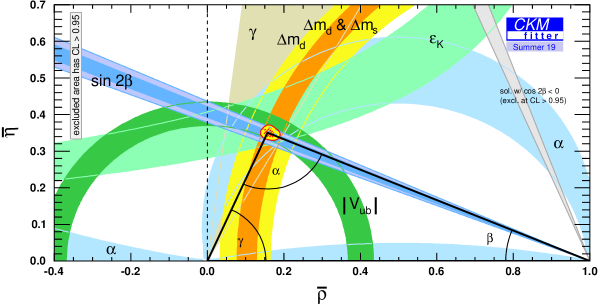
Figure 6: Experimental constraints on the SM unitarity triangle [111].

We have already determined the sides of the unitarity triangle in Eqs. (64) and (87), through two ${\cal CP}$-conserving observables: $|\mathbf{V}_{\!ub}/\mathbf{V}_{\!cb}|$ and $B^{0}_{d,s}$ mixing. This gives the circular rings shown in Fig. 6, centered at the vertices $(0,0)$ and $(1,0)$. Their overlap at $\eta\not=0$ establishes that ${\cal CP}$ is violated (assuming unitarity). More direct constraints on the parameter $\eta$ can be obtained from ${\cal CP}$-violating observables, which provide sensitivity to the angles of the unitarity triangle ($\alpha+\beta+\gamma=\pi$):

$$\alpha\equiv\arg{\left[-{\mathbf{V}^{\phantom{*}}_{\!td}\mathbf{V}^{*}_{\!tb}\over\mathbf{V}^{\phantom{*}}_{\!ud}\mathbf{V}^{*}_{\!ub}}\right]}\,,\qquad\quad\beta\equiv\arg{\left[-{\mathbf{V}^{\phantom{*}}_{\!cd}\mathbf{V}^{*}_{\!cb}\over\mathbf{V}^{\phantom{*}}_{\!td}\mathbf{V}^{*}_{\!tb}}\right]}\,,\qquad\quad\gamma\equiv\arg{\left[-{\mathbf{V}^{\phantom{*}}_{\!ud}\mathbf{V}^{*}_{\!ub}\over\mathbf{V}^{\phantom{*}}_{\!cd}\mathbf{V}^{*}_{\!cb}}\right]}\,.$$ (92)

6.1 Indirect and direct ${\cal CP}$ violation in the kaon system

Any observable ${\cal CP}$-violation effect is generated by the interference between different amplitudes contributing to the same physical transition. This interference can occur either through meson-antimeson mixing or via final-state interactions, or by a combination of both effects.

The flavour-specific decays $K^{0}\to\pi^{-}\ell^{+}\nu_{\ell}$ and $\bar{K}^{0}\to\pi^{+}\ell^{-}\bar{\nu}_{\ell}$ provide a way to measure the departure of the $K^{0}$–$\bar{K}^{0}$ mixing parameter $|p/q|$ from unity. In the SM, the decay amplitudes satisfy $|A(\bar{K}^{0}\to\pi^{+}\ell^{-}\bar{\nu}_{\ell})|=|A(K^{0}\to\pi^{-}\ell^{+}\nu_{\ell})|$; therefore ($\ell=e,\mu$),

$$A_{L}\,\equiv\,{\Gamma(K_{L}\to\pi^{-}\ell^{+}\nu_{\ell})-\Gamma(K_{L}\to\pi^{+}\ell^{-}\bar{\nu}_{\ell})\over\Gamma(K_{L}\to\pi^{-}\ell^{+}\nu_{\ell})+\Gamma(K_{L}\to\pi^{+}\ell^{-}\bar{\nu}_{\ell})}\,=\,{|p|^{2}-|q|^{2}\over|p|^{2}+|q|^{2}}\,=\,{2\,\mathrm{Re}\,(\bar{\varepsilon}^{\phantom{{}^{\prime}}}_{K})\over(1+|\bar{\varepsilon}^{\phantom{{}^{\prime}}}_{K}|^{2})}\,.$$ (93)

The experimental measurement [9], $A_{L}=(3.32\pm 0.06)\cdot 10^{-3}$, implies

$$\mathrm{Re}\,(\bar{\varepsilon}^{\phantom{{}^{\prime}}}_{K})\,=\,(1.66\pm 0.03)\cdot 10^{-3}\,,$$ (94)

which establishes the presence of indirect ${\cal CP}$ violation generated by the mixing amplitude.

If the flavour of the decaying meson $P$ is known, any observed difference between the decay rate $\Gamma(P\to f)$ and its ${\cal CP}$ conjugate $\Gamma(\bar{P}\to\bar{f})$ would indicate that ${\cal CP}$ is directly violated in the decay amplitude. One could study, for instance, ${\cal CP}$ asymmetries in decays such as $K^{\pm}\to\pi^{\pm}\pi^{0}$ where the pion charges identify the kaon flavour; however, no positive signals have been found in charged kaon decays. Since at least two interfering contributions are needed, let us write the decay amplitudes as

$$A[P\to f]\,=\,M_{1}\,e^{i\phi_{1}}\,e^{i\delta_{1}}\,+\,M_{2}\,e^{i\phi_{2}}\,e^{i\delta_{2}}\,,\qquad\;A[\bar{P}\to\bar{f}]\,=\,M_{1}\,e^{-i\phi_{1}}e^{i\delta_{1}}\,+\,M_{2}\,e^{-i\phi_{2}}e^{i\delta_{2}}\,,$$ (95)

where $\phi_{i}$ denote weak phases, $\delta_{i}$ strong final-state interaction phases and $M_{i}$ the moduli of the matrix elements. Notice that the weak phase gets reversed under ${\cal CP}$, while the strong one remains of course invariant. The rate asymmetry is given by

$$\mathcal{A}_{P\to f}^{{\cal CP}}\,\equiv\,{\Gamma[P\to f]-\Gamma[\bar{P}\to\bar{f}]\over\Gamma[P\to f]+\Gamma[\bar{P}\to\bar{f}]}\;=\;{-2M_{1}M_{2}\,\sin{(\phi_{1}-\phi_{2})}\,\sin{(\delta_{1}-\delta_{2})}\over|M_{1}|^{2}+|M_{2}|^{2}+2M_{1}M_{2}\,\cos{(\phi_{1}-\phi_{2})}\,\cos{(\delta_{1}-\delta_{2})}}\,.$$ (96)

Thus, to generate a direct ${\cal CP}$ asymmetry one needs: 1) at least two interfering amplitudes, which should be of comparable size in order to get a sizeable asymmetry; 2) two different weak phases [$\sin{(\phi_{1}-\phi_{2})}\not=0$],  and  3) two different strong phases [$\sin{(\delta_{1}-\delta_{2})}\not=0$].

Direct ${\cal CP}$ violation has been searched for in decays of neutral kaons, where $K^{0}$–$\bar{K}^{0}$ mixing is also involved. Thus, both direct and indirect ${\cal CP}$ violation need to be taken into account simultaneously. A ${\cal CP}$-violation signal is provided by the ratios:

$$\eta_{+-}\,\equiv\,{A(K_{L}\to\pi^{+}\pi^{-})\over A(K_{S}\to\pi^{+}\pi^{-})}\,=\,\varepsilon_{K}^{\phantom{{}^{\prime}}}+\varepsilon_{K}^{\prime}\,,\qquad\qquad\eta_{00}\,\equiv\,{A(K_{L}\to\pi^{0}\pi^{0})\over A(K_{S}\to\pi^{0}\pi^{0})}\,=\,\varepsilon_{K}^{\phantom{{}^{\prime}}}-2\varepsilon_{K}^{\prime}\,.$$ (97)

The dominant effect from ${\cal CP}$ violation in $K^{0}$–$\bar{K}^{0}$ mixing is contained in $\varepsilon_{K}^{\phantom{{}^{\prime}}}$, while $\varepsilon_{K}^{\prime}$ accounts for direct ${\cal CP}$ violation in the decay amplitudes [42]:

$$\varepsilon_{K}^{\phantom{{}^{\prime}}}=\bar{\varepsilon}_{K}^{\phantom{{}^{\prime}}}+i\xi_{0}\,,\qquad\varepsilon_{K}^{\prime}={i\over\sqrt{2}}\,\omega\,(\xi_{2}-\xi_{0})\,,\qquad\omega\equiv{\mathrm{Re}\,(A_{2})\over\mathrm{Re}\,(A_{0})}\,e^{i(\delta_{2}-\delta_{0})}\,,\qquad\xi_{I}\equiv{\mathrm{Im}\,(A_{I})\over\mathrm{Re}\,(A_{I})}\,.$$ (98)

$A_{I}$ are the transition amplitudes into two pions with isospin $I=0,2$ (these are the only two values allowed by Bose symmetry for the final $2\pi$ state) and $\delta_{I}$ their corresponding strong phase shifts. Although $\varepsilon_{K}^{\prime}$ is strongly suppressed by the small ratio $|\omega|\approx 1/22$, a non-zero value has been established through very accurate measurements, demonstrating the existence of direct ${\cal CP}$ violation in K decays [112, 113, 114, 115]:

$$\mathrm{Re}\left(\varepsilon_{K}^{\prime}/\varepsilon_{K}^{\phantom{{}^{\prime}}}\right)=\frac{1}{3}\left(1-\left|\frac{\eta_{{}_{00}}}{\eta_{{}_{+-}}}\right|\right)=\,(16.6\pm 2.3)\cdot 10^{-4}\,.$$ (99)

In the SM the necessary weak phases are generated through the gluonic and electroweak penguin diagrams shown in Fig. 7, involving virtual up-type quarks of the three generations in the loop. These short-distance contributions are known to NLO in the strong coupling [116, 117]. However, the theoretical prediction involves a delicate balance between the two isospin amplitudes and is sensitive to long-distance and isospin-violating effects. Using chiral perturbation theory techniques, one finds $\mathrm{Re}\left(\varepsilon_{K}^{\prime}/\varepsilon_{K}^{\phantom{{}^{\prime}}}\right)=(14\pm 5)\cdot 10^{-4}$ [118, 119, 120, 121, 122], in agreement with (99) but with a large uncertainty.

Figure 7: $\Delta S=1$ penguin diagrams.

Since $\mathrm{Re}\left(\varepsilon_{K}^{\prime}/\varepsilon_{K}^{\phantom{{}^{\prime}}}\right)\ll 1$, the ratios $\eta_{{}_{+-}}$ and $\eta_{{}_{00}}$ provide a measurement of $\varepsilon_{K}^{\phantom{{}^{\prime}}}=|\varepsilon_{K}^{\phantom{{}^{\prime}}}|\,\mbox{\rm e}^{i\phi_{\varepsilon}}$ [9]:

$$|\varepsilon_{K}^{\phantom{{}^{\prime}}}|\,=\,\frac{1}{3}\left(2|\eta_{{}_{+-}}|+|\eta_{{}_{00}}|\right)\,=\,(2.228\pm 0.011)\cdot 10^{-3},\qquad\qquad\phi_{\varepsilon}\,=\,(43.52\pm 0.05)^{\circ}\,,$$ (100)

in perfect agreement with the semileptonic asymmetry $A_{L}$. In the SM $\varepsilon_{K}^{\phantom{{}^{\prime}}}$ receives short-distance contributions from box diagrams involving virtual top and charm quarks, which are proportional to

$$\varepsilon_{K}^{\phantom{{}^{\prime}}}\,\propto\,\sum_{i,j=c,t}\,\eta_{ij}\;\mathrm{Im}\!\left[\mathbf{V}_{\!id}^{\phantom{*}}\mathbf{V}_{\!is}^{*}\mathbf{V}_{\!jd}^{\phantom{*}}\mathbf{V}_{\!js}^{*}\right]\,S(r_{i},r_{j})\;\propto\;A^{2}\lambda^{6}\bar{\eta}\,\left\{\eta_{tt}\,A^{2}\lambda^{4}(1-\bar{\rho})+P_{c}\right\}\,.$$ (101)

The first term shows the CKM dependence of the dominant top contribution, $P_{c}$ accounts for the charm corrections [124] and the short-distance QCD corrections $\eta_{ij}$ are known to NLO [107, 108, 125]. The measured value of $|\varepsilon_{K}^{\phantom{{}^{\prime}}}|$ determines an hyperbolic constraint in the $(\bar{\rho},\bar{\eta})$ plane, shown in Fig. 6, taking into account the theoretical uncertainty in the hadronic matrix element of the $\Delta S=2$ operator [39].

6.2 ${\cal CP}$ asymmetries in B decays

The semileptonic decays  $B_{q}^{0}\to X^{-}\ell^{+}\nu_{\ell}$  and  $\bar{B}^{0}_{q}\to X^{+}\ell^{-}\bar{\nu}_{\ell}$  ($q=d,s$) provide the most direct way to measure the amount of ${\cal CP}$ violation in the $B^{0}$–$\bar{B}^{0}$ mixing matrix, through

$$a_{\mathrm{sl}}^{q} \equiv \frac{\Gamma(\bar{B}^{0}_{q}\to X^{-}\ell^{+}\nu_{\ell})-\Gamma(B^{0}_{q}\to X^{+}\ell^{-}\bar{\nu}_{\ell})}{\Gamma(\bar{B}^{0}_{q}\to X^{-}\ell^{+}\nu_{\ell})+\Gamma(B^{0}_{q}\to X^{+}\ell^{-}\bar{\nu}_{\ell})}\;=\;{|p|^{4}-|q|^{4}\over|p|^{4}+|q|^{4}}\;\approx\,4\;\mathrm{Re}\,(\bar{\varepsilon}_{B_{q}^{0}})$$ (102)

$$\approx \frac{|\Gamma_{12}|}{|M_{12}|}\,\sin{\phi_{q}}\;\approx\;\frac{|\Delta\Gamma_{B^{0}_{q}}|}{|\Delta M_{B^{0}_{q}}|}\,\tan{\phi_{q}}\,.$$

This asymmetry is expected to be tiny because $|\Gamma_{12}/M_{12}|\sim m_{b}^{2}/m_{t}^{2}\ll 1$. Moreover, there is an additional GIM suppression in the relative mixing phase $\phi_{q}\equiv\arg{\left(-M_{12}/\Gamma_{12}\right)}\sim(m_{c}^{2}-m_{u}^{2})/m_{b}^{2}$, implying a value of $|q/p|$ very close to 1. Therefore, $a_{\mathrm{sl}}^{q}$ could be very sensitive to new sources of ${\cal CP}$ violation beyond the SM, contributing to $\phi_{q}$. The present measurements give [9, 46]

$$\mathrm{Re}(\bar{\varepsilon}_{B_{d}^{0}})\,=\,(-0.5\pm 0.4)\cdot 10^{-3}\,,\qquad\qquad\mathrm{Re}(\bar{\varepsilon}_{B_{s}^{0}})\,=\,(-0.15\pm 0.70)\cdot 10^{-3}\,.$$ (103)

The large $B^{0}$–$\bar{B}^{0}$ mixing provides a different way to generate the required ${\cal CP}$-violating interference. There are quite a few nonleptonic final states which are reachable both from a $B^{0}$ and a $\bar{B}^{0}$. For these flavour non-specific decays the $B^{0}$ (or $\bar{B}^{0}$) can decay directly to the given final state $f$, or do it after the meson has been changed to its antiparticle via the mixing process; there are two different amplitudes, $A(B^{0}\to f)$ and $A(B^{0}\to\bar{B}^{0}\to f)$, corresponding to two possible decay paths. ${\cal CP}$-violating effects can then result from the interference of these two contributions.

The time-dependent decay probabilities for the decay of a neutral $B$ meson created at the time $t_{0}=0$ as a pure $B^{0}$ ($\bar{B}^{0}$) into the final state $f$  ($\bar{f}\equiv{\cal CP}\,f$) are:

$$\Gamma[B^{0}(t)\to f] \!\!\propto \!\!{1\over 2}\,e^{-\Gamma_{B^{0}}t}\,\left(|A_{f}|^{2}+|\bar{A}_{f}|^{2}\right)\,\left\{1+C_{f}\,\cos{(\Delta M_{B^{0}}t)}-S_{f}\,\sin{(\Delta M_{B^{0}}t)}\right\}\,,$$

$$\Gamma[\bar{B}^{0}(t)\to\bar{f}] \!\!\propto \!\!{1\over 2}\,e^{-\Gamma_{B^{0}}t}\,\left(|\bar{A}_{\bar{f}}|^{2}+|A_{\bar{f}}|^{2}\right)\,\left\{1-C_{\bar{f}}\,\cos{(\Delta M_{B^{0}}t)}+S_{\bar{f}}\,\sin{(\Delta M_{B^{0}}t)}\right\}\,,\quad$$ (104)

where the tiny $\Delta\Gamma_{B^{0}}$ corrections have been neglected and we have introduced the notation

$$A_{f}\equiv A[B^{0}\to f]\,,\qquad\qquad\bar{A}_{f}\equiv-A[\bar{B}^{0}\to f]\,,\qquad\qquad\bar{\rho}_{f}\equiv\bar{A}_{f}/A_{f}\,,$$

$$A_{\bar{f}}\equiv A[B^{0}\to\bar{f}]\,,\qquad\qquad\bar{A}_{\bar{f}}\equiv-A[\bar{B}^{0}\to\bar{f}]\,,\qquad\qquad\rho_{\bar{f}}\equiv A_{\bar{f}}/\bar{A}_{\bar{f}}\,,$$ (105)

$$C_{f}\equiv\frac{1-|\bar{\rho}_{f}|^{2}}{1+|\bar{\rho}_{f}|^{2}}\,,\qquad\quad S_{f}\equiv\frac{2\,\mathrm{Im}\left({q\over p}\,\bar{\rho}_{f}\right)}{1+|\bar{\rho}_{f}|^{2}}\,,\qquad\quad C_{\bar{f}}\equiv-\frac{1-|\rho_{\bar{f}}|^{2}}{1+|\rho_{\bar{f}}|^{2}}\,,\qquad\quad S_{\bar{f}}\equiv\frac{-2\,\mathrm{Im}\left({p\over q}\,\rho_{\bar{f}}\right)}{1+|\rho_{\bar{f}}|^{2}}\,.$$

${\cal CP}$ invariance demands the probabilities of ${\cal CP}$-conjugate processes to be identical. Thus, ${\cal CP}$ conservation requires $A_{f}=\bar{A}_{\bar{f}}$, $A_{\bar{f}}=\bar{A}_{f}$, $\bar{\rho}_{f}=\rho_{\bar{f}}$ and $\mathrm{Im}({q\over p}\,\bar{\rho}_{f})=\mathrm{Im}({p\over q}\,\rho_{\bar{f}})$, $C_{f}=-C_{\bar{f}}$ and $S_{f}=-S_{\bar{f}}$. Violation of any of the first three equalities would be a signal of direct ${\cal CP}$ violation. The fourth equality tests ${\cal CP}$ violation generated by the interference of the direct decay $B^{0}\to f$ and the mixing-induced decay $B^{0}\to\bar{B}^{0}\to f$.

For $B^{0}$ mesons

$$\left.{q\over p}\right|_{B^{0}_{q}}\;\approx\;\sqrt{{M_{12}^{*}\over M_{12}}}\;\approx\;{\mathbf{V}_{\!\!tb}^{*}\mathbf{V}_{\!\!tq}^{\phantom{*}}\over\mathbf{V}_{\!\!tb}^{\phantom{*}}\mathbf{V}_{\!\!tq}^{*}}\;\equiv\;e^{-2i\phi^{M}_{q}}\,,$$ (106)

where $\phi^{M}_{d}=\beta+{\cal O}(\lambda^{4})$ and $\phi^{M}_{s}=-\beta_{s}+{\cal O}(\lambda^{6})$. The angle $\beta$ is defined in Eq. (92), while $\beta_{s}\equiv\arg{\left[-\left(\mathbf{V}^{\phantom{*}}_{\!ts}\mathbf{V}^{*}_{\!tb}\right)/\left(\mathbf{V}^{\phantom{*}}_{\!cs}\mathbf{V}^{*}_{\!cb}\right)\right]}=\lambda^{2}\eta+{\cal O}(\lambda^{4})$ is the equivalent angle in the $B^{0}_{s}$ unitarity triangle, which is predicted to be tiny. Therefore, the mixing ratio $q/p$ is given by a known weak phase.

An obvious example of final states $f$ which can be reached both from the $B^{0}$ and the $\bar{B}^{0}$ are ${\cal CP}$ eigenstates; states such that $\bar{f}=\zeta_{f}f$  ($\zeta_{f}=\pm 1$). In this case, $A_{\bar{f}}=\zeta_{f}A_{f}$, $\bar{A}_{\bar{f}}=\zeta_{f}\bar{A}_{f}$, $\rho_{\bar{f}}=1/\bar{\rho}_{f}$, $C_{\bar{f}}=C_{f}$ and $S_{\bar{f}}=S_{f}$. A non-zero value of $C_{f}$ or $S_{f}$ signals then ${\cal CP}$ violation. The ratios $\bar{\rho}_{f}$ and $\rho_{\bar{f}}$ depend in general on the underlying strong dynamics. However, for ${\cal CP}$ self-conjugate final states, all dependence on the strong interaction disappears if only one weak amplitude contributes to the $B^{0}\to f$ and $\bar{B}^{0}\to f$ transitions [126, 127]. In this case, we can write the decay amplitude as $A_{f}=Me^{i\phi^{D}}\!e^{i\delta_{s}}$, with $M=M^{*}$ and $\phi^{D}$ and $\delta_{s}$ weak and strong phases. The ratios $\bar{\rho}_{f}$ and $\rho_{\bar{f}}$ are then given by

$$\rho_{\bar{f}}\,=\,\bar{\rho}_{f}^{*}\,=\,\zeta_{f}\,e^{2i\phi^{D}}\,.$$ (107)

The modulus $M$ and the unwanted strong phase cancel out completely from these two ratios; $\rho_{\bar{f}}$ and $\bar{\rho}_{f}$ simplify to a single weak phase, associated with the underlying weak quark transition. Since $|\rho_{\bar{f}}|=|\bar{\rho}_{f}|=1$, the time-dependent decay probabilities become much simpler. In particular, $C_{f}=0$ and there is no longer any dependence on  $\cos{(\Delta M_{B^{0}}t)}$. Moreover, the coefficients of the sinusoidal terms are then fully known in terms of CKM mixing angles only: $S_{f}=S_{\bar{f}}=-\zeta_{f}\sin{[2(\phi^{M}_{q}+\phi^{D})]}\equiv-\zeta_{f}\sin{(2\Phi)}$. In this ideal case, the time-dependent ${\cal CP}$-violating decay asymmetry

$${\cal A}^{{\cal CP}}_{\bar{B}^{0}\to\bar{f}}\,\equiv\,{\Gamma[\bar{B}^{0}(t)\to\bar{f}]-\Gamma[B^{0}(t)\to f]\over\Gamma[\bar{B}^{0}(t)\to\bar{f}]+\Gamma[B^{0}(t)\to f]}\;=\;-\zeta_{f}\sin{(2\Phi)}\,\sin{(\Delta M_{B^{0}}t)}$$ (108)

provides a direct and clean measurement of the CKM parameters [128].

When several decay amplitudes with different phases contribute, $|\bar{\rho}_{f}|\not=1$ and the interference term will depend both on CKM parameters and on the strong dynamics embodied in $\bar{\rho}_{f}$. The leading contributions to $\bar{b}\to\bar{q}^{\prime}q^{\prime}\bar{q}$ are either the tree-level $W$ exchange or penguin topologies generated by gluon ($\gamma$, $Z$) exchange. Although of higher order in the strong (electroweak) coupling, penguin amplitudes are logarithmically enhanced by the virtual $W$ loop and are potentially competitive. Table 3 contains the CKM factors associated with the two topologies for different $B$ decay modes into ${\cal CP}$ eigenstates.

Table 3: CKM factors and relevant angle $\Phi$ for some $B$ decays into ${\cal CP}$ eigenstates.

Decay	Tree-level CKM	Penguin CKM	Exclusive channels	$\Phi$
$\bar{b}\to\bar{c}c\bar{s}$	$A\lambda^{2}$	$-A\lambda^{2}$	$B^{0}_{d}\to J/\psi\,K_{S},J/\psi\,K_{L}$	$\beta$
			$B^{0}_{s}\to D_{s}^{+}D_{s}^{-},J/\psi\,\phi$	$-\beta_{s}$
$\bar{b}\to\bar{s}s\bar{s}$		$-A\lambda^{2}$	$B^{0}_{d}\to K_{S}\phi,K_{L}\phi$	$\beta$
			$B^{0}_{s}\to\phi\phi$	$-\beta_{s}$
$\bar{b}\to\bar{d}d\bar{s}$		$-A\lambda^{2}$	$B^{0}_{s}\to K_{S}K_{S},K_{L}K_{L}$	$-\beta_{s}$
$\bar{b}\to\bar{c}c\bar{d}$	$-A\lambda^{3}$	$A\lambda^{3}(1-\rho-i\eta)$	$B^{0}_{d}\to D^{+}D^{-},J/\psi\,\pi^{0}$	$\approx\beta$
			$B^{0}_{s}\to J/\psi\,K_{S},J/\psi\,K_{L}$	$\approx-\beta_{s}$
$\bar{b}\to\bar{u}u\bar{d}$	$A\lambda^{3}(\rho+i\eta)$	$A\lambda^{3}(1-\rho-i\eta)$	$B^{0}_{d}\to\pi^{+}\pi^{-},\rho^{0}\pi^{0},\omega\pi^{0}$	$\approx\beta+\gamma$
			$B^{0}_{s}\to\rho^{0}K_{S,L},\omega K_{S,L},\pi^{0}K_{S,L}$	$\not=\gamma-\beta_{s}$
$\bar{b}\to\bar{s}s\bar{d}$		$A\lambda^{3}(1-\rho-i\eta)$	$B^{0}_{d}\to K_{S}K_{S},K_{L}K_{L},\phi\pi^{0}$	0
			$B^{0}_{s}\to K_{S}\phi,K_{L}\phi$	$-\beta-\beta_{s}$

The gold-plated decay mode is $B^{0}_{d}\to J/\psi\,K_{S}$. In addition of having a clean experimental signature, the two topologies have the same (zero) weak phase. The ${\cal CP}$ asymmetry provides then a clean measurement of the mixing angle $\beta$, without strong-interaction uncertainties. Fig. 8 shows the Belle measurement [129] of time-dependent $\bar{b}\to c\bar{c}\bar{s}$ asymmetries for ${\cal CP}$-odd ($B^{0}_{d}\to J/\psi\,K_{S}$, $B^{0}_{d}\to\psi^{\prime}K_{S}$, $B^{0}_{d}\to\chi_{c1}K_{S}$) and ${\cal CP}$-even ($B^{0}_{d}\to J/\psi\,K_{L}$) final states. A very nice oscillation is manifest, with opposite signs for the two different choices of $\zeta_{f}=\pm 1$. Including the information obtained from other $\bar{b}\to c\bar{c}\bar{s}$ decays, one gets the world average [46]:

$$\sin{(2\beta)}=0.699\pm 0.017\,.$$ (109)

Fitting an additional $\cos{(\Delta M_{B^{0}}t)}$ term in the measured asymmetries results in $C_{f}=-0.005\pm 0.015$ [46], confirming the expected null result. An independent measurement of $\sin{2\beta}$ can be obtained from $\bar{b}\to s\bar{s}\bar{s}$ and $\bar{b}\to d\bar{d}\bar{s}$ decays, which only receive penguin contributions and, therefore, could be more sensitive to new-physics corrections in the loop diagram. These modes give  $\sin{(2\beta)}=0.648\pm 0.038$ [46], in good agreement with (109).

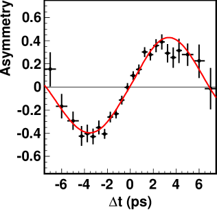
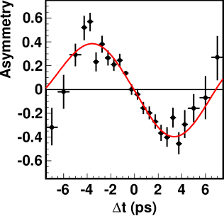
Figure 8: Time-dependent asymmetries for ${\cal CP}$-odd ($B^{0}_{d}\to J/\psi\,K_{S}$, $B^{0}_{d}\to\psi^{\prime}K_{S}$, $B^{0}_{d}\to\chi_{c1}K_{S}$; $\zeta_{f}=-1$; left) and ${\cal CP}$-even ($B^{0}_{d}\to J/\psi\,K_{L}$; $\zeta_{f}=+1$; right) final states, measured by Belle [129].

Eq. (109) determines the angle $\beta$ up to a four-fold ambiguity: $\beta$, $\frac{\pi}{2}-\beta$, $\pi+\beta$ and $\frac{3\pi}{2}-\beta$. The solution $\beta=(22.2\pm 0.7)^{\circ}$ is in remarkable agreement with the other phenomenological constraints on the unitarity triangle in Fig. 6. The ambiguity has been resolved through a time-dependent analysis of the Dalitz plot distribution in $B^{0}_{d}\to D^{(*)}h^{0}$ decays ($h^{0}=\pi^{0},\eta,\omega$), showing that $\cos{(2\beta)}=0.91\pm 0.25$ and $\beta=(22.5\pm 4.6)^{\circ}$[130]. This proves that $\cos{(2\beta)}$ is positive with a $3.7\,\sigma$ significance, while the multifold solution $\frac{\pi}{2}-\beta=(67.8\pm 0.7)^{\circ}$ is excluded at the $7.3\,\sigma$ level.

A determination of $\beta+\gamma=\pi-\alpha$ can be obtained from $\bar{b}\to\bar{u}u\bar{d}$ decays, such as $B^{0}_{d}\to\pi\pi$ or $B^{0}_{d}\to\rho\rho$. However, the penguin contamination that carries a different weak phase can be sizeable. The time-dependent asymmetry in $B^{0}_{d}\to\pi^{+}\pi^{-}$ shows indeed a non-zero value for the $\cos{(\Delta M_{B^{0}}t)}$ term, $C_{f}=-0.32\pm 0.04$ [46], providing evidence of direct ${\cal CP}$ violation and indicating the presence of an additional decay amplitude; therefore, $S_{f}=-0.63\pm 0.04\not=\sin{2\alpha}$. One could still extract useful information on $\alpha$ (up to 16 mirror solutions), using the isospin relations among the $B^{0}_{d}\to\pi^{+}\pi^{-}$, $B^{0}_{d}\to\pi^{0}\pi^{0}$ and $B^{+}\to\pi^{+}\pi^{0}$ amplitudes and their ${\cal CP}$ conjugates [131]; however, only a loose constraint is obtained, given the limited experimental precision on $B^{0}_{d}\to\pi^{0}\pi^{0}$. Much stronger constraints are obtained from $B^{0}_{d}\to\rho^{+}\rho^{-},\rho^{0}\rho^{0}$ because one can use the additional polarization information of two vectors in the final state to resolve the different contributions and, moreover, the small branching fraction $\mathrm{Br}(B^{0}_{d}\to\rho^{0}\rho^{0})=(9.6\pm 1.5)\cdot 10^{-7}$ [9] implies a very small penguin contribution. Additional information can be obtained from $B^{0}_{d},\bar{B}^{0}_{d}\to\rho^{\pm}\pi^{\mp},a_{1}^{\pm}\pi^{\mp}$, although the final states are not ${\cal CP}$ eigenstates. Combining all pieces of information results in [46]

$$\alpha\,=\,(84.9\,{}^{+\,5.1}_{-\,4.5})^{\circ}\,.$$ (110)

The angle $\gamma$ cannot be determined in $\bar{b}\to u\bar{u}\bar{d}$ decays such as $B_{s}^{0}\to\rho^{0}K_{S}$ because the colour factors in the hadronic matrix element enhance the penguin amplitude with respect to the tree-level contribution. Instead, $\gamma$ can be measured through the tree-level decays $B\to D^{(*)}K^{(*)}$ ($\bar{b}\to\bar{u}c\bar{s}$) and $B\to\bar{D}^{(*)}K^{(*)}$ ($\bar{b}\to\bar{c}u\bar{s}$), using final states accessible in both $D^{(*)0}$ and $\bar{D}^{(*)0}$ decays and playing with the interference of both amplitudes [132, 133, 134]. The sensitivity can be optimized with Dalitz-plot analyses of the $D^{0},\bar{D}^{0}$ decay products. The extensive experimental studies performed so far result in [46]

$$\gamma\,=\,(71.1\,{}^{+\,4.6}_{-\,5.3})^{\circ}\,.$$ (111)

Another ambiguous solution with $\gamma\leftrightarrow\gamma+\pi$ also exists.

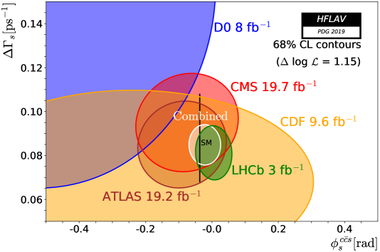
Figure 9: 68% CL regions in $\Delta\Gamma_{B^{0}_{s}}$ and $\phi_{s}^{c\bar{c}s}$, extracted from $\,\bar{b}\to\bar{c}c\bar{s}$ $\,{\cal CP}$ asymmetries of $B^{0}_{s}$ mesons [46]. The vertical black line shows the SM prediction [135, 136, 137].

Mixing-induced ${\cal CP}$ violation has been also searched for in the decays of $B^{0}_{s}$ and $\bar{B}^{0}_{s}$ mesons into $J/\psi\,\phi,\psi(2\mathrm{S})\phi,J/\psi\,K^{+}K^{-},J/\psi\,\pi^{+}\pi^{-}$ and $D_{s}^{+}D_{s}^{-}$. From the corresponding time-dependent ${\cal CP}$ asymmetries, one extracts correlated constraints on $\Delta\Gamma_{s}$ and the weak phase $\phi_{s}^{c\bar{c}s}\equiv 2\Phi_{s}^{c\bar{c}s}\approx 2\phi^{M}_{s}\approx-2\beta_{s}$ in Eq. (108), which are shown in Fig. 9. They lead to [46]

$$\beta_{s}\;=\;(0.60\pm 0.89)^{\circ}\,,$$ (112)

in good agreement with the SM prediction $\beta_{s}\approx\eta\lambda^{2}\approx 1^{\circ}$.

6.3 Global fit of the unitarity triangle

The CKM parameters can be more accurately determined through a global fit to all available measurements, imposing the unitarity constraints and taking properly into account the theoretical uncertainties. The global fit shown in Fig. 6 uses frequentist statistics and gives [111]

$$\lambda\,=\,0.22484\,{}^{+\,0.00025}_{-\,0.00006}\,,\qquad A\,=\,0.824\,{}^{+\,0.006}_{-\,0.015}\,,\qquad\bar{\rho}\,=\,0.157\,{}^{+\,0.010}_{-\,0.006}\,,\qquad\bar{\eta}\,=\,0.350\,{}^{+\,0.008}_{-\,0.007}\,.$$ (113)

This implies ${\cal J}=(3.06\,{}^{+\,0.07}_{-\,0.08})\cdot 10^{-5}$, $\alpha=(91.7\,{}^{+\,1.7}_{-\,1.1})^{\circ}$, $\beta=(22.6\,{}^{+\,0.5}_{-\,0.4})^{\circ}$ and $\gamma=(65.8\,{}^{+\,0.9}_{-\,1.3})^{\circ}$. Similar results are obtained by the UTfit group [138], using instead a Bayesian approach and a slightly different treatment of theoretical uncertainties.

6.4 Direct ${\cal CP}$ violation in $B$ decays

The big data samples accumulated at the $B$ factories and the collider experiments have established the presence of direct ${\cal CP}$ violation in several decays of $B$ mesons. The most significative signals are [9, 46]

$${\cal A}^{{\cal CP}}_{\bar{B}^{0}_{d}\to K^{-}\pi^{+}}=-0.083\pm 0.004\,,\qquad{\cal A}^{{\cal CP}}_{\bar{B}^{0}_{d}\to\bar{K}^{*0}\eta}=0.19\pm 0.05\,,\qquad{\cal A}^{{\cal CP}}_{\bar{B}^{0}_{d}\to K^{*-}\pi^{+}}=-0.27\pm 0.04\,,$$

$$C_{B^{0}_{d}\to\pi^{+}\pi^{-}}=-0.32\pm 0.04\,,\qquad\;\gamma_{B\to D^{(*)}K^{(*)}}=(71.1\,{}^{+\,4.6}_{-\,5.3})^{\circ}\,,\qquad\;{\cal A}^{{\cal CP}}_{\bar{B}^{0}_{s}\to K^{+}\pi^{-}}=0.221\pm 0.015\,,$$

$${\cal A}^{{\cal CP}}_{B^{-}\to K^{-}\rho^{0}}=0.37\pm 0.10\,,\qquad{\cal A}^{{\cal CP}}_{B^{-}\to K^{-}\eta}=-0.37\pm 0.08\,,\qquad{\cal A}^{{\cal CP}}_{B^{-}\to\pi^{-}\pi^{+}\pi^{-}}=0.057\pm 0.013\,,$$

$${\cal A}^{{\cal CP}}_{B^{-}\to K^{-}K^{+}K^{-}}=-0.033\pm 0.008\,,\qquad\qquad\qquad{\cal A}^{{\cal CP}}_{B^{-}\to K^{-}K^{+}\pi^{-}}=-0.122\pm 0.021\,.$$

$${\cal A}^{{\cal CP}}_{B^{-}\to K^{-}f_{2}(1270)}=-0.68\,{}^{+\,0.19}_{-\,0.17}\,,\qquad\qquad\qquad{\cal A}^{{\cal CP}}_{B^{-}\to\pi^{-}f_{2}(1270)}=0.40\pm 0.06\,,$$ (114)

Another prominent observation of direct ${\cal CP}$ violation has been done recently in charm decays [139]:

$${\cal A}^{\mathrm{direct}\;{\cal CP}}_{D^{0}\to K^{-}K^{+}}-{\cal A}^{\mathrm{direct}\;{\cal CP}}_{D^{0}\to\pi^{-}\pi^{+}}\,=\,(-15.7\pm 2.9)\cdot 10^{-4}\,,$$ (115)

where the small contribution from $D^{0}$–$\bar{D}^{0}$ mixing has been subtracted, using the measured difference of reconstructed mean decay times of the two modes. Unfortunately, owing to the unavoidable presence of strong phases, a real theoretical understanding of the corresponding SM predictions is still lacking. Progress in this direction is needed to perform meaningful tests of the CKM mechanism of ${\cal CP}$ violation and pin down any possible effects from new physics beyond the SM framework.

7 Rare decays

Complementary and very valuable information can be obtained from rare decays that in the SM are strongly suppressed by the GIM mechanism. These processes are then sensitive to new-physics contributions with a different flavour structure. Well-known examples are the $\bar{K}^{0}\to\mu^{+}\mu^{-}$ decay modes [9, 140],

$$\mathrm{Br}(K_{L}\to\mu^{+}\mu^{-})\,=\,(6.84\pm 0.11)\cdot 10^{-9}\,,\qquad\qquad\mathrm{Br}(K_{S}\to\mu^{+}\mu^{-})\,<\,2.1\cdot 10^{-10}\quad(90\%\>\mathrm{CL})\,,$$ (116)

which tightly constrain any hypothetical flavour-changing ($s\to d$) tree-level coupling of the $Z$ boson. In the SM, these decays receive short-distance contributions from the penguin and box diagrams displayed in Fig. 10. Owing to the unitarity of the CKM matrix, the resulting amplitude vanishes for equal up-type quark masses, which entails a heavy suppression:

$${\cal M}\,\propto\,\sum_{i=u,c,t}\mathbf{V}_{\!is}\mathbf{V}_{\!id}^{*}\;F(m_{i}^{2}/M_{W}^{2})\,=\,\mathbf{V}_{\!cs}\mathbf{V}_{\!cd}^{*}\;\tilde{F}(m_{c}^{2}/M_{W}^{2})+\mathbf{V}_{\!ts}\mathbf{V}_{\!td}^{*}\;\tilde{F}(m_{t}^{2}/M_{W}^{2})\,,$$ (117)

where $F(x)$ is a loop function and  $\tilde{F}(x)\equiv F(x)-F(0)$. In addition to the loop factor $g^{4}/(16\pi^{2})$, the charm contribution carries a mass suppression $\lambda m_{c}^{2}/M_{W}^{2}$, while the top term is proportional to $\lambda^{5}A^{2}(1-\rho+i\eta)\,m_{t}^{2}/M_{W}^{2}$. The large top mass compensates the strong Cabibbo suppression so that the top contribution is finally larger than the charm one. However, the total short-distance contribution to the $K_{L}$ decay, $\mathrm{Br}(K_{L}\to\mu^{+}\mu^{-})_{\rm\scriptstyle sd}=(0.79\pm 0.12)\cdot 10^{-9}$ [141, 124], is nearly one order of magnitude below the experimental measurement (116), while $\mathrm{Br}(K_{S}\to\mu^{+}\mu^{-})_{\rm\scriptstyle sd}\approx 1.7\cdot 10^{-13}$ [42].

The decays $K_{L}\to\mu^{+}\mu^{-}$ and $K_{S}\to\mu^{+}\mu^{-}$ are actually dominated by long-distance contributions, through  $K_{L}\to\pi^{0},\eta,\eta^{\prime}\to\gamma\gamma\to\mu^{+}\mu^{-}$  and  $K_{S}\to\pi^{+}\pi^{-}\to\gamma\gamma\to\mu^{+}\mu^{-}$. The absorptive component from two on-shell intermediate photons nearly saturates the measured $\mathrm{Br}(K_{L}\to\mu^{+}\mu^{-})$ [142], while the $K_{S}$ decay rate is predicted to be $\mathrm{Br}(K_{S}\to\mu^{+}\mu^{-})=5.1\cdot 10^{-12}$ [42, 143]. These decays can be rigorously analised with chiral perturbation theory techniques [42], but the strong suppression of their short-distance contributions does not make possible to extract useful information on the CKM parameters. Nevertheless, it is possible to predict the longitudinal polarization $P_{L}$ of either muon in the $K_{L}$ decay, a ${\cal CP}$-violating observable which in the SM is dominated by indirect ${\cal CP}$ violation from $K^{0}$–$\bar{K}^{0}$ mixing: $|P_{L}|=(2.6\pm 0.4)\cdot 10^{-3}$ [143].

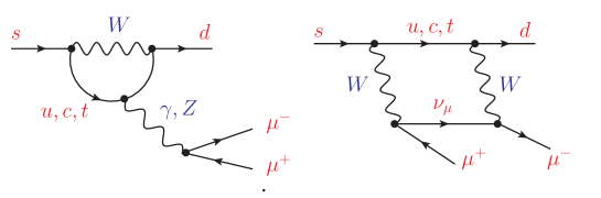
Figure 10: Short-distance penguin (left) and box (right) SM contributions to $\bar{K}^{0}\to\mu^{+}\mu^{-}$.

Other interesting kaon decay modes such as $K^{0}\to\gamma\gamma$, $K\to\pi\gamma\gamma$ and $K\to\pi\ell^{+}\ell^{-}$ are also governed by long-distance physics [42, 144]. Of particular interest is the decay $K_{L}\to\pi^{0}e^{+}e^{-}$, since it is sensitive to new sources of ${\cal CP}$ violation. At lowest order in $\alpha$ the decay proceeds through $K_{2}^{0}\to\pi^{0}\gamma^{*}$ that violates ${\cal CP}$, while the ${\cal CP}$-conserving contribution through $K_{L}^{0}\to\pi^{0}\gamma^{*}\gamma^{*}$ is suppressed by an additional power of $\alpha$ and it is found to be below $10^{-12}$ [42]. The $K_{L}\to\pi^{0}e^{+}e^{-}$ transition is then dominated by the ${\cal O}(\alpha)$ ${\cal CP}$-violating contributions [144], both from $K^{0}$–$\bar{K}^{0}$ mixing and direct ${\cal CP}$ violation. The estimated rate $\mathrm{Br}(K_{L}\to\pi^{0}e^{+}e^{-})=(3.1\pm 0.9)\cdot 10^{-11}$ [42, 145, 146] is only a factor ten smaller than the present (90% CL) upper bound of $2.8\cdot 10^{-10}$ [147] and should be reachable in the near future.

The decays $K^{\pm}\to\pi^{\pm}\nu\bar{\nu}$ and $K_{L}\to\pi^{0}\nu\bar{\nu}$ provide a more direct access to CKM information because long-distance effects play a negligible role. The decay amplitudes are dominated by $Z$-penguin and $W$-box loop diagrams of the type shown in Fig. 10 (replacing the final muons by neutrinos), and are proportional to the hadronic $K\pi$ matrix element of the $\Delta S=1$ vector current, which (assuming isospin symmetry) is extracted from $K\to\pi\ell\nu_{\ell}$ decays. The small long-distance and isospin-violating corrections can be estimated with chiral perturbation theory. The neutral decay is ${\cal CP}$ violating and proceeds almost entirely through direct ${\cal CP}$ violation (via interference with mixing). Taking the CKM inputs from other observables, the predicted SM rates are [148, 149, 150]:

$$\mathrm{Br}(K^{+}\to\pi^{+}\nu\bar{\nu})_{\mathrm{th}}=(8.5\pm 0.6)\cdot 10^{-11}\,,\qquad\qquad\mathrm{Br}(K_{L}\to\pi^{0}\nu\bar{\nu})_{\mathrm{th}}=(2.9\pm 0.3)\cdot 10^{-11}\,.$$ (118)

The uncertainties are largely parametrical, due to CKM input, the charm and top masses and $\alpha_{s}(M_{Z})$. On the experimental side, the current upper bounds on the charged [151] and neutral [152] modes are

$$\mathrm{Br}(K^{+}\to\pi^{+}\nu\bar{\nu})<1.85\cdot 10^{-10}\,,\qquad\qquad\mathrm{Br}(K_{L}\to\pi^{0}\nu\bar{\nu})<3.0\cdot 10^{-9}\quad(90\%\,{\rm CL}).$$ (119)

The ongoing CERN NA62 experiment aims to reach ${\cal O}(100)$ $K^{+}\to\pi^{+}\nu\bar{\nu}$ events (assuming SM rates), while increased sensitivities on the $K_{L}\to\pi^{0}\nu\bar{\nu}$ mode are expected to be achieved by the KOTO experiment at J-PARC. These experiments will start to seriously probe the new-physics potential of these decays.

The inclusive decay $\bar{B}\to X_{s}\gamma$ provides another powerful test of the SM flavour structure at the quantum loop level. It proceeds through a $b\to s\gamma$ penguin diagram with an on-shell photon. The present experimental world average, $\mathrm{Br}(\bar{B}\to X_{s}\gamma)_{E_{\gamma}\geq 1.6~{}\mathrm{GeV}}=(3.32\pm 0.15)\cdot 10^{-4}$ [46], agrees very well with the SM theoretical prediction, $\mathrm{Br}(\bar{B}\to X_{s}\gamma)_{E_{\gamma}\geq 1.6~{}\mathrm{GeV}}^{\mathrm{th}}=(3.40\pm 0.17)\cdot 10^{-4}$ [153, 154, 155], obtained at the next-to-next-to-leading order.

The LHC experiments have recently reached the SM sensitivity for the $B_{d}^{0}$ and $B_{s}^{0}$ decays into $\mu^{+}\mu^{-}$ pairs [156, 157, 158]. The current world averages [9],

$$\overline{\mathrm{Br}}(B^{0}_{d}\to\mu^{+}\mu^{-})\,=\,(1.4\,{}^{+\,1.6}_{-\,1.4})\cdot 10^{-10}\,,\qquad\qquad\overline{\mathrm{Br}}(B_{s}^{0}\to\mu^{+}\mu^{-})\,=\,(3.0\pm 0.4)\cdot 10^{-9}\,,$$ (120)

agree with the SM predictions $\overline{\mathrm{Br}}(B_{d}^{0}\to\mu^{+}\mu^{-})=(1.06\pm 0.09)\cdot 10^{-10}$ and $\overline{\mathrm{Br}}(B_{s}^{0}\to\mu^{+}\mu^{-})=(3.65\pm 0.23)\cdot 10^{-9}$ [160]. Other interesting FCNC decays with $B$ mesons are $\bar{B}\to K^{(*)}l^{+}l^{-}$ and $\bar{B}\to K^{(*)}\nu\bar{\nu}$ [86].

8 Flavour constraints on new physics

The CKM matrix provides a very successful description of flavour phenomena, as it is clearly exhibited in the unitarity test of Fig. 6, showing how very different observables converge into a single choice of CKM parameters. This is a quite robust and impressive result. One can perform separate tests with different subsets of measurements, according to their ${\cal CP}$-conserving or ${\cal CP}$-violating nature, or splitting them into tree-level and loop-induced processes. In all cases, one finally gets a closed triangle and similar values for the fitted CKM entries [111, 138]. However, the SM mechanism of flavour mixing and ${\cal CP}$ violation is conceptually quite unsatisfactory because it does not provide any dynamical understanding of the numerical values of fermion masses, and mixings. We completely ignore the reasons why the fermion spectrum contains such a hierarchy of different masses, spanning many orders of magnitude, and which fundamental dynamics is behind the existence of three flavour generations and their observed mixing structure.

The phenomenological success of the SM puts severe constraints on possible scenarios of new physics. The absence of any clear signals of new phenomena in the LHC searches is pushing the hypothetical new-physics scale at higher energies, above the TeV. The low-energy implications of new dynamics beyond the SM can then be analysed in terms of an effective Lagrangian, containing only the known SM fields:

$${\cal L}_{\rm\scriptstyle eff}\,=\,L_{\rm\scriptstyle SM}\,+\,\sum_{d>4}\sum_{k}\,\frac{c_{k}^{(d)}}{\Lambda_{\rm\scriptstyle NP}^{d-4}}\;O_{k}^{(d)}\,.$$ (121)

The effective Lagrangian is organised as an expansion in terms of dimension-$d$ operators $O_{k}^{(d)}$, invariant under the SM gauge group, suppressed by the corresponding powers of the new-physics scale $\Lambda_{\rm\scriptstyle NP}$. The dimensionless couplings $c_{k}^{(d)}$ encode information on the underlying dynamics. The lowest-order term in this dimensional expansion is the SM Lagrangian that contains all allowed operators of dimension 4.

At low energies, the terms with lower dimensions dominate the physical transition amplitudes. There is only one operator with $d=5$ (up to Hermitian conjugation and flavour assignments), which violates lepton number by two units and is then related with the possible existence of neutrino Majorana masses [161]. Taking $m_{\nu}\;\lower 3.0pt\hbox{$\buildrel>\over{\sim}$}\;0.05$ eV, one estimates a very large lepton-number-violating scale $\Lambda_{\rm\scriptstyle NP}/c^{(5)}\;\lower 3.0pt\hbox{$\buildrel<\over{\sim}$}\;10^{15}$ GeV [17]. Assuming lepton-number conservation, the first signals of new phenomena should be associated with $d=6$ operators.

One can easily analyse the possible impact of $\Delta F=2$ ($F=S,C,B$) four-quark operators ($d=6$), such as the SM left-left operator in Eq. (85) that induces a $\Delta B=2$ transition. Since the SM box diagram provides an excellent description of the data, hypothetical new-physics contributions can only be tolerated within the current uncertainties, which puts stringent upper bounds on the corresponding Wilson coefficients $\tilde{c}_{k}\equiv c_{k}^{(6)}/\Lambda_{\rm\scriptstyle NP}^{2}$. For instance, $\Delta M_{B^{0}_{d}}$ and $S_{J/\psi K_{S}}$ imply that the real (${\cal CP}$-conserving) and imaginary (${\cal CP}$-violating) parts of $\tilde{c}_{k}$ must be below $10^{-6}\;\mathrm{TeV}^{-2}$ for a $(\bar{b}_{L}\gamma^{\mu}d_{L})^{2}$ operator, and nearly one order of magnitude smaller ($10^{-7}$) for $(\bar{b}_{R}d_{L})(\bar{b}_{L}d_{R})$ [162]. Stronger bounds are obtained in the kaon system from $\Delta M_{K^{0}}$ and $\varepsilon_{K}$. For the $(\bar{s}_{L}\gamma^{\mu}d_{L})^{2}$ operator the real (imaginary) coefficient must be below $10^{-6}$ ($3\cdot 10^{-9}$), while the corresponding bounds for $(\bar{s}_{R}d_{L})(\bar{s}_{L}d_{R})$ are $7\cdot 10^{-9}$ ($3\cdot 10^{-11}$), in the same TeV^-2 units [162]. Taking the coefficients $c_{k}^{(6)}\sim{\cal O}(1)$, this would imply $\Lambda_{\rm\scriptstyle NP}>3\cdot 10^{3}$ TeV for $B^{0}_{d}$ and $\Lambda_{\rm\scriptstyle NP}>3\cdot 10^{5}$ TeV for $K^{0}$. Therefore, two relevant messages emerge from the data:

1. A generic flavour structure with coefficients $c_{k}^{(6)}\sim{\cal O}(1)$ is completely ruled out at the TeV scale.

2. New flavour-changing physics at $\Lambda_{\rm\scriptstyle NP}\sim 1$ TeV could only be possible if the corresponding Wilson coefficients $c_{k}^{(6)}$ inherit the strong SM suppressions generated by the GIM mechanism.

The last requirement can be satisfied by assuming that the up and down Yukawa matrices are the only sources of quark-flavour symmetry breaking (minimal flavour violation) [163, 164, 165]. In the absence of Yukawa interactions, the SM Lagrangian has a ${\cal G}\equiv U(3)_{L_{L}}\otimes U(3)_{Q_{L}}\otimes U(3)_{\ell_{R}}\otimes U(3)_{u_{R}}\otimes U(3)_{d_{R}}$ global flavour symmetry, because one can rotate arbitrarily in the 3-generation space each one of the five SM fermion components in Eq. (2). The Yukawa matrices are the only explicit breakings of this large symmetry group. Assuming that the new physics does not introduce any additional breakings of the flavour symmetry ${\cal G}$ (beyond insertions of Yukawa matrices), one can easily comply with the flavour bounds. Otherwise, flavour data provide very strong constraints on models with additional sources of flavour symmetry breaking and probe physics at energy scales not directly accessible at accelerators.

The subtle SM cancellations suppressing FCNC transitions could be easily destroyed in the presence of new physics contributions. To better appreciate the non-generic nature of the flavour structure, let us analyse the simplest extension of the SM scalar sector with a second Higgs doublet, which increases the number of quark Yukawas:

$${\cal L}_{Y}\,=\,-\sum_{a=1}^{2}\left\{\bar{Q}_{L}^{\prime}\,{\cal Y}^{(a)\raisebox{3.0pt}{$\scriptscriptstyle\prime$}}_{d}\phi_{a}\,d^{\prime}_{R}+\bar{Q}_{L}^{\prime}\,{\cal Y}^{(a)\raisebox{3.0pt}{$\scriptscriptstyle\prime$}}_{u}\phi^{c}_{a}\,u^{\prime}_{R}+\bar{L}^{\prime}_{L}\,{\cal Y}^{(a)\raisebox{3.0pt}{$\scriptscriptstyle\prime$}}_{\ell}\phi_{a}\,\ell^{\prime}_{R}\right\}\,+\,\mathrm{h.c.}\,,$$ (122)

where $\phi_{a}^{T}=(\phi_{a}^{(+)},\phi_{a}^{(0)})$ are the two scalar doublets, $\phi_{a}^{c}$ their ${\cal C}$-conjugate fields, and $Q^{\prime}_{L}$ and $L^{\prime}_{L}$ the left-handed quark and lepton doublets, respectively. All fermion fields are written as three-dimensional flavour vectors and ${\cal Y}^{(a)\raisebox{3.0pt}{$\scriptscriptstyle\prime$}}_{f}$ are $3\times 3$ complex matrices in flavour space. With an appropriate scalar potential, the neutral components of the scalar doublets acquire vacuum expectation values $\langle 0|\phi_{a}^{(0)}|0\rangle=v_{a}\,\mbox{\rm e}^{i\theta_{a}}$. It is convenient to make a $U(2)$ transformation in the space of scalar fields, $(\phi_{1},\phi_{2})\to(\Phi_{1},\Phi_{2})$, so that only the first doublet has a non-zero vacuum expectation value $v=(v_{1}^{2}+v_{2}^{2})^{1/2}$. $\Phi_{1}$ plays then the same role as the SM Higgs doublet, while $\Phi_{2}$ does not participate in the electroweak symmetry breaking. In this scalar basis the Yukawa interactions become more transparent:

$$\sum_{a=1}^{2}{\cal Y}^{(a)\raisebox{3.0pt}{$\scriptscriptstyle\prime$}}_{d,\ell}\,\phi_{a}\,=\,\sum_{a=1}^{2}Y^{(a)\raisebox{3.0pt}{$\scriptscriptstyle\prime$}}_{d,\ell}\,\Phi_{a}\,,\qquad\qquad\qquad\sum_{a=1}^{2}{\cal Y}^{(a)\raisebox{3.0pt}{$\scriptscriptstyle\prime$}}_{u}\,\phi^{c}_{a}\,=\,\sum_{a=1}^{2}Y^{(a)\raisebox{3.0pt}{$\scriptscriptstyle\prime$}}_{u}\,\Phi^{c}_{a}\,.$$ (123)

The fermion masses originate from the $\Phi_{1}$ couplings, because $\Phi_{1}$ is the only field acquiring a vacuum expectation value:

$$M_{f}^{\prime}\,=\,Y^{(1)\raisebox{3.0pt}{$\scriptscriptstyle\prime$}}_{f}\;\frac{v}{\sqrt{2}}\,.$$ (124)

The diagonalization of these fermion mass matrices proceeds in exactly the same way as in the SM, and defines the fermion mass eigenstates $d_{i}$, $u_{i}$, $\ell_{i}$, with diagonal mass matrices $M_{f}$, as described in Section 2. However, in general, one cannot diagonalize simultaneously all Yukawa matrices, in the fermion mass-eigenstate basis the matrices $Y_{f}^{(2)}$ remain non-diagonal, giving rise to dangerous flavour-changing transitions mediated by neutral scalars. The appearance of FCNC interactions represents a major phenomenological shortcoming, given the very strong experimental bounds on this type of phenomena.

To avoid this disaster, one needs to implement ad-hoc dynamical restrictions to guarantee the suppression of FCNC couplings at the required level. Unless the Yukawa couplings are very small or the scalar bosons very heavy, a specific flavour structure is required by the data. The unwanted non-diagonal neutral couplings can be eliminated requiring the alignment in flavour space of the Yukawa matrices [166]:

$$Y^{(2)}_{d,\ell}\,=\,\varsigma_{d,\ell}\,Y^{(1)}_{d,\ell}\,=\,\frac{\sqrt{2}}{v}\,\varsigma_{d,\ell}\,M_{d,\ell}\,,\qquad\qquad\qquad Y^{(2)}_{u}\,=\,\varsigma_{u}^{*}\,Y^{(1)}_{u}\,=\,\frac{\sqrt{2}}{v}\,\varsigma_{u}^{*}\,M_{u}\,,$$ (125)

with $\varsigma_{f}$ arbitrary complex proportionality parameters.

Flavour alignment constitutes a very simple implementation of minimal flavour violation. It results in a very specific dynamical structure, with all fermion-scalar interactions being proportional to the corresponding fermion masses. The Yukawas are fully characterized by the three complex alignment parameters $\varsigma_{f}$, which introduce new sources of ${\cal CP}$ violation. The aligned two-Higgs doublet model Lagrangian satisfies the flavour constraints [168, 169, 170, 171, 172, 173, 174, 175, 176, 177, 178], and leads to a rich collider phenomenology with five physical scalar bosons [179, 180, 181, 182, 183, 184, 185, 186]: $h$, $H$, $A$ and $H^{\pm}$.

9 Flavour anomalies

The experimental data exhibit a few deviations from the SM predictions [187]. For instance, Table 2 shows a $2.6\,\sigma$ violation of lepton universality in $|g_{\tau}/g_{\mu}|$ at the 1% level, from $W\to\ell\nu$ decays, that is difficult to reconcile with the precise 0.15% limits extracted from virtual $W^{\pm}$ transitions, shown also in the same table. In fact, it has been demonstrated that it is not possible to accommodate this deviation from universality with an effective Lagrangian and, therefore, such a signal could only be explained by the introduction of new light degrees of freedom that so far remain undetected [188]. Thus, the most plausible explanation is a small problem (statistical fluctuation or underestimated systematics) in the LEP-2 measurements that will remain unresolved until more precise high-statistics $W\to\ell\nu$ data samples become available.

Some years ago BaBar reported a non-zero ${\cal CP}$ asymmetry in $\tau^{\pm}\to\pi^{\pm}K_{S}\nu$ decays at the level of $3.6\cdot 10^{-3}$ [189], the same size than the SM expectation from $K^{0}$–$\bar{K}^{0}$ mixing [190, 191] but with the opposite sign, which represents a $2.8\,\sigma$ anomaly. So far, Belle has only reached a null result with a smaller $10^{-2}$ sensitivity and, therefore, has not been able to either confirm or refute the asymmetry. Nevertheless, on very general grounds, it has been shown that the BaBar signal is incompatible with other sets of data ($K^{0}$ and $D^{0}$ mixing, neutron electric dipole moment) [192].

Another small flavour anomaly was triggered by the unexpected large value of $\mathrm{Br}(B^{-}\to\tau^{-}\bar{\nu})$, found in 2006 by Belle [193] and later confirmed by BaBar [96], which implied values of $|\mathbf{V}_{\!ub}|$ higher than the ones measured in semileptonic decays or extracted from global CKM fits. While the BaBar results remain unchanged, the reanalysis of the full Belle data sample resulted in a sizeable $\sim 40\%$ reduction of the measured central value [97], eliminating the discrepancy with the SM but leaving a pending disagreement with the BaBar results.

In the last few years a series of anomalies have emerged in $b\to c\tau\nu$ and $b\to s\mu^{+}\mu^{-}$ transitions. Given the difficulty of the experimental analyses, the results should be taken with some caution and further studies with larger data sets are still necessary. Nevertheless, these anomalies exhibit a quite consistent pattern that makes them intriguing.

9.1 $b\to c\tau\nu$ decays

In 2012 the BaBar collaboration [194] observed an excess in $B\to D^{(*)}\tau\nu_{\tau}$ decays with respect to the SM predictions [195], indicating a violation of lepton-flavour universality at the 30% level. The measured observables are the ratios

$$R(D)\,\equiv\,\frac{\mathrm{Br}(B\to D\tau\nu)}{\mathrm{Br}(B\to D\ell\nu)}\,,\qquad\qquad\qquad R(D^{*})\,\equiv\,\frac{\mathrm{Br}(B\to D^{*}\tau\nu)}{\mathrm{Br}(B\to D^{*}\ell\nu)}\,,$$ (126)

with $\ell=e,\mu$, where many sources of experimental and theoretical errors cancel. The effect has been later confirmed by LHCb [196] ($D^{*}$ mode only) and Belle [197] (Fig. 11). Although the results of the last two experiments are slightly closer to the SM expected values, $R(D)=0.302\pm 0.004$ and $R(D^{*})=0.258\,{}^{+\,0.006}_{-\,0.005}$ [55, 58, 198, 199, 200, 201, 202], the resulting world averages [46]

$$R(D)\,=\,0.340\pm 0.027\pm 0.013\,,\qquad\qquad R(D^{*})\,=\,0.295\pm 0.011\pm 0.008\,,$$ (127)

deviate at the $3.2\,\sigma$ level (considering their correlation of $-0.38$) from the SM predictions, which is a very large effect for a tree-level SM transition.

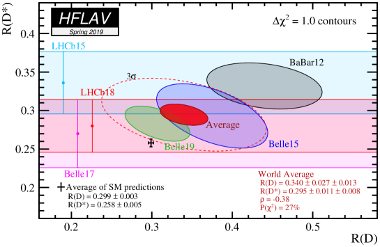
Figure 11: Measurements of $R(D)$ and $R(D^{*})$ and their average compared with the SM predictions. Filled contours correspond to $\Delta\chi^{2}=1$ (68% CL for the bands and 39% CL for the ellipses), while the dashed ellipse displays the $3\,\sigma$ region [46].

Different new-physics explanations of the anomaly have been put forward: new charged vector or scalar bosons, leptoquarks, right-handed neutrinos, etc. The normalized $q^{2}$ distributions measured by BaBar [194] and Belle [197] do not favour large deviations from the SM [203]. One must also take into account that the needed enhancement of the $b\to c\tau\nu$ transition is constrained by the cross-channel $b\bar{c}\to\tau\nu$. A conservative (more stringent) upper bound $\mathrm{Br}(B_{c}\to\tau\nu)<30\%$ (10%) can be extracted from the $B_{c}$ lifetime [203, 204] (LEP data [205]). A global fit to the data, using a generic low-energy effective Hamiltonian with four-fermion effective operators [201, 202], finds several viable possibilities. However, while the fitted results clearly indicate that new-physics contributions are needed (much lower $\chi^{2}$ than in the SM), they don’t show any strong preference for a particular Wilson coefficient. The simplest solution would be some new-physics contribution that only manifests in the Wilson coefficient of the SM operator $(\bar{c}_{L}\gamma^{\mu}b_{L})(\bar{\tau}_{L}\gamma_{\mu}\nu_{L})$. This would imply a universal enhancement of all $b\to c\tau\nu$ transitions, in agreement with the recent LHCb observation of the $B_{c}\to J/\psi\,\tau\nu$ decay [206],

$$R(J/\psi)\,\equiv\,\frac{\mathrm{Br}(B_{c}\to J/\psi\,\tau\nu)}{\mathrm{Br}(B_{c}\to J/\psi\,\ell\nu)}\,=\,0.71\pm 0.17\pm 0.18\,,$$ (128)

which is $2\,\sigma$ above the SM expected value  $R(J/\psi)\sim 0.25$–0.28 [207, 208, 209, 210]. Writing the four-fermion left-left operator in terms of $SU(2)_{L}\otimes U(1)_{Y}$ invariant operators at the electroweak scale, and imposing that the experimental bounds on $\mathrm{Br}(b\to s\nu\bar{\nu})$ are satisfied, this possibility would imply rather large rates in $b\to s\tau^{+}\tau^{-}$ transitions [211, 212, 213], but still safely below the current upper limits [214].

9.2 $b\to s\ell^{+}\ell^{-}$ decays

The rates of several $b\to s\mu^{+}\mu^{-}$ transitions have been found at LHCb to be consistently lower than their SM predictions: $B^{+}\to K^{+}\mu^{+}\mu^{-}$ [215, 216], $B^{+}\to K^{*+}\mu^{+}\mu^{-}$ [215], $B^{0}_{d}\to K^{0}\mu^{+}\mu^{-}$ [215], $B^{0}_{d}\to K^{*0}\mu^{+}\mu^{-}$ [217], $B_{s}^{0}\to\phi\mu^{+}\mu^{-}$ [218] and $\Lambda^{0}_{b}\rightarrow\Lambda\mu^{+}\mu^{-}$ [219]. The angular and invariant-mass distributions of the final products in $B\to K^{*}\mu^{+}\mu^{-}$ have been also studied by ATLAS [220], BaBar [221], Belle [222], CDF [223], CMS [224] and LHCb [217]. The rich variety of angular dependences in the four-body $K\pi\mu^{+}\mu^{-}$ final state allows one to disentangle different sources of dynamical contributions. Particular attention has been put in the so-called optimised observables $P^{\prime}_{i}(q^{2})$, where $q^{2}$ is the dilepton invariant-mass squared, which are specific combinations of angular observables that are free from form-factor uncertainties in the heavy quark-mass limit [225]. A sizeable discrepancy with the SM prediction [226, 227, 228], shown in Fig. 12, has been identified in two adjacent bins of the $P^{\prime}_{5}$ distribution, just below the $J/\Psi$ peak. Belle has also included $K^{*}e^{+}e^{-}$ final states in the analysis, but the results for this electron mode are compatible with the SM expectations [222].

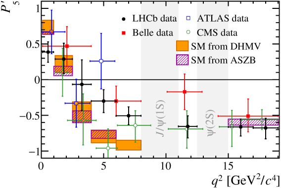
Figure 12: Comparison between the SM predictions for $P^{\prime}_{5}$ [226, 227, 228] and the experimental measurements [229].

The SM predictions for the previous observables suffer from hadronic uncertainties that are not easy to quantify. However, LHCb has also reported sizeable violations of lepton flavour universality, at the $2.1$-$2.6\,\sigma$ level, through the ratios [230]

$$R_{K^{*0}}\,\equiv\,\frac{\mathrm{Br}(B^{0}_{d}\to K^{*0}\mu^{+}\mu^{-})}{B^{0}_{d}\to K^{*0}e^{+}e^{-})}\,=\,\left\{\begin{array}[]{ccc}0.66\,{}^{+\,0.11}_{-\,0.07}\pm 0.03\,,&&q^{2}\in\,[0.045\,,\,1.1]\;\mathrm{GeV}^{2}\,,\\[5.0pt] 0.69\,{}^{+\,0.11}_{-\,0.07}\pm 0.05\,,&&q^{2}\in\,[1.1\,,\,6.0]\;\mathrm{GeV}^{2}\,,\end{array}\right.$$ (129)

and [231]

$$R_{K}\,\equiv\,\left.\frac{\mathrm{Br}(B^{+}\to K^{+}\mu^{+}\mu^{-})}{\mathrm{Br}(B^{+}\to K^{+}e^{+}e^{-})}\right|_{q^{2}\in\,[1.1\,,\,6.0]\;\mathrm{GeV}^{2}}\,=\,0.846\,{}^{+\,0.060}_{-\,0.054}\,{}^{+\,0.016}_{-\,0.014}\,.$$ (130)

These observables constitute a much cleaner probe of new physics because most theoretical uncertainties cancel out [232, 233, 234, 235]. In the SM, the only difference between the muon and electron channels is the lepton mass. The SM theoretical predictions, $R_{K}=1.00\pm 0.01_{\rm\scriptstyle QED}$, $R_{K^{*0}}[0.045,1.1]=0.906\pm 0.028_{\rm\scriptstyle th}$ and $R_{K^{*0}}[1.1,6]=1.00\pm 0.01_{\rm\scriptstyle QED}$ [236], deviate from these experimental measurements by $2.4\,\sigma$, $2.1\,\sigma$ and $2.6\,\sigma$, respectively. Owing to their larger uncertainties, the recent Belle measurements of $R_{K^{*}}$ [237] and $R_{K}$ [238] are compatible with the SM as well as with LHCb.

Global fits to the $b\to s\ell^{+}\ell^{-}$ data with an effective low-energy Lagrangian

$${\cal L}_{\rm\scriptstyle eff}\,=\,\frac{G_{F}}{\sqrt{2}}\,\mathbf{V}_{\!tb}\mathbf{V}_{\!ts}^{*}\,\frac{\alpha}{\pi}\;\sum_{i,\ell}\,C_{i,\ell}\,O_{i}^{\ell}$$ (131)

show a clear preference for new-physics contributions to the operators $O_{9}^{\ell}=(\bar{s}_{L}\gamma_{\mu}b_{L})(\bar{\ell}\gamma^{\mu}\ell)$ and $O_{10}^{\ell}=(\bar{s}_{L}\gamma_{\mu}b_{L})(\bar{\ell}\gamma^{\mu}\gamma_{5}\ell)$, with $\ell=\mu$ [239, 240, 241, 242, 243, 244, 245]. Although the different analyses tend to favour slightly different solutions, two main common scenarios stand out: either $\delta C_{9,\mu}^{\mathrm{NP}}\approx-0.98$ or $\delta C_{9,\mu}^{\mathrm{NP}}=-\delta C_{10,\mu}^{\mathrm{NP}}\approx-0.46$. Both constitute large shifts ($-24\%$ and $-11\%$, respectively) from the SM values: $C_{9,\mu}^{\mathrm{SM}}(\mu_{b})\approx 4.1$ and $C_{10,\mu}^{\mathrm{SM}}(\mu_{b})\approx-4.3$, at $\mu_{b}=4.8$ GeV. The first possibility is slightly preferred by the global analysis of all data, while the left-handed new-physics solution accommodates better the lepton-flavour-universality-violating observables [240].

The left-handed scenario is theoretically appealing because it can be easily generated through $SU(2)_{L}\otimes U(1)_{Y}$-invariant effective operators at the electroweak scale that, moreover, could also provide an explanation to the $b\to c\tau\nu$ anomaly. This possibility emerges naturally from the so-called $U_{1}$ vector leptoquark model [246], and can be tested experimentally, since it implies a $b\to s\tau^{+}\tau^{-}$ rate three orders of magnitude larger than the SM expectation [213]. For a recent review of theoretical models with a quite complete list of references, see Ref. [247].

10 Discussion

The flavour structure of the SM is one of the main pending questions in our understanding of weak interactions. Although we do not know the reasons of the observed family replication, we have learnt experimentally that the number of SM generations is just three (and no more). Therefore, we must study as precisely as possible the few existing flavours, to get some hints on the dynamics responsible for their observed structure.

In the SM all flavour dynamics originate in the fermion mass matrices, which determine the measurable masses and mixings. Thus, flavour is related through the Yukawa interactions with the scalar sector, the part of the SM Lagrangian that is more open to theoretical speculations. At present, we totally ignore the underlying dynamics responsible for the vastly different scales exhibited by the fermion spectrum and the particular values of the measured mixings. The SM Yukawa matrices are just a bunch of arbitrary parameters to be fitted to data, which is conceptually unsatisfactory.

The SM incorporates a mechanism to generate ${\cal CP}$ violation, through the single phase naturally occurring in the CKM matrix. This mechanism, deeply rooted into the unitarity structure of $\mathbf{V}$, implies very specific requirements for ${\cal CP}$ violation to show up. The CKM matrix has been thoroughly investigated in dedicated experiments and a large number of ${\cal CP}$-violating processes have been studied in detail. The flavour data seem to fit into the SM framework, confirming that the fermion mass matrices are the dominant source of flavour-mixing phenomena. However, a fundamental explanation of the flavour dynamics is still lacking.

At present, a few flavour anomalies have been identified in $b\to c\tau\nu$ and $b\to s\mu^{+}\mu^{-}$ transitions. Whether they truly represent the first signals of new phenomena, or just result from statistical fluctuations and/or underestimated systematics remains to be understood. New experimental input from LHC and Belle-II should soon clarify the situation. Very valuable information on the flavour dynamics is also expected from BESS-III and from several kaon (NA62, KOTO) and muon (MEG-II, Mu2e, Mu3e, COMET) experiments, complementing the high-energy searches for new phenomena at LHC. Unexpected surprises may well be discovered, probably giving hints of new physics at higher scales and offering clues to the problems of fermion mass generation, quark mixing and family replication.

Appendix A Conservation of the vector current

In the limit where all quark masses are equal, the QCD Lagrangian remains invariant under global $SU(N_{f})$ transformations of the quark fields in flavour space, where $N_{f}$ is the number of (equal-mass) quark flavours. This guarantees the conservation of the corresponding Noether currents  $V^{\mu}_{ij}=\bar{u}_{i}\gamma^{\mu}d_{j}$. In fact, using the QCD equations of motion, one immediately finds that

$$\partial_{\mu}V^{\mu}_{ij}\,\equiv\,\partial_{\mu}\left(\bar{u}_{i}\gamma^{\mu}d_{j}\right)\,=\,i\,\bigl{(}m_{u_{i}}-m_{d_{j}}\bigr{)}\,\bar{u}_{i}d_{j}\,,$$ (132)

which vanishes when $m_{u_{i}}=m_{d_{j}}$. In momentum space, this reads  $q_{\mu}V^{\mu}_{ij}={\cal O}(m_{u_{i}}-m_{d_{j}})$, with $q_{\mu}$ the corresponding momentum transfer.

Let us consider a $0^{-}(k)\to 0^{-}(k^{\prime})$ weak transition mediated by the vector current $V^{\mu}_{ij}$. The relevant hadronic matrix element is given in Eq. (39) and contains two form factors $f_{\pm}(q^{2})$. The conservation of the vector current implies that $f_{-}(q^{2})$ is identically zero when $m_{u_{i}}=m_{d_{j}}$. Therefore,

$$\langle P^{\prime}_{i}(k^{\prime})|V^{\mu}_{ij}(x)|P_{j}(k)\rangle\,=\,\mbox{\rm e}^{iq\cdot x}\;C_{PP^{\prime}}\;(k+k^{\prime})^{\mu}\;f_{+}(q^{2})\,.$$ (133)

We have made use of translation invariance to write  $V^{\mu}_{ij}(x)=\mbox{\rm e}^{iP\cdot x}\,V^{\mu}_{ij}(0)\,\mbox{\rm e}^{-iP\cdot x}$, with $P^{\mu}$ the four-momentum operator. This determines the dependence of the matrix element on the space-time coordinate, with $q^{\mu}=(k^{\prime}-k)^{\mu}$.

The conserved Noether charges

$${\cal N}_{ij}\,=\,\int d^{3}x\;V^{0}_{ij}(x)\,=\,\int d^{3}x\;u_{i}^{\dagger}(x)\,d_{j}(x)\,,$$ (134)

annihilate one quark $d_{j}$ and create instead one $u_{i}$ (or replace $\bar{u}_{i}$ by $\bar{d}_{j}$), transforming the meson $P$ into $P^{\prime}$ (up to a trivial Clebsh-Gordan factor $C_{PP^{\prime}}$ that, for light-quarks, takes the value $1/\sqrt{2}$ when $P^{\prime}$ is a $\pi^{0}$ and is 1 otherwise). Thus,

$$\langle P^{\prime}(k^{\prime})|{\cal N}_{ij}|P(k)\rangle\,=\,C_{PP^{\prime}}\;\langle P^{\prime}(k^{\prime})|P^{\prime}(k)\rangle\,=\,C_{PP^{\prime}}\;(2\pi)^{3}\;2k^{0}\;\delta^{(3)}(\vec{k}^{\prime}-\vec{k}\,)\,.$$ (135)

On the other side, inserting in this matrix element the explicit expression for ${\cal N}_{ij}$ in (134) and making use of (133),

$$\langle P^{\prime}(k^{\prime})|{\cal N}_{ij}|P(k)\rangle\,=\,\int d^{3}x\;\langle P^{\prime}(k^{\prime})|V^{0}_{ij}(x)|P(k)\rangle\,=\,C_{PP^{\prime}}\;(2\pi)^{3}\;2k^{0}\;\delta^{(3)}(\vec{q}\,)\;f_{+}(0)\,.$$ (136)

Comparing Eqs. (135) and (136), one finally obtains the result

$$f_{+}(0)\,=\,1\,.$$ (137)

Therefore, the flavour symmetry $SU(N_{f})$ determines the normalization of the form factor at $q^{2}=0$, when $m_{u_{i}}=m_{d_{j}}$. It is possible to prove that the deviations from 1 are of second order in the symmetry-breaking quark mass difference, $f_{+}(0)=1+{\cal O}[(m_{u_{i}}-m_{d_{j}})^{2}]$ [25].

References

- [1] S.L. Glashow, Nucl. Phys. 22 (1961) 579.
- [2] S. Weinberg, Phys. Rev. Lett. 19 (1967) 1264.
- [3] A. Salam, in Elementary Particle Theory, ed. N. Svartholm (Almquist and Wiksells, Stockholm, 1969), p. 367.
- [4] A. Pich, The Standard Model of Electroweak Interactions, Reports CERN-2006-003 and CERN-2007-005, ed. R. Fleischer, p. 1; arXiv:hep-ph/0502010, arXiv:0705.4264 [hep-ph].
- [5] A. Pich, Flavour Physics and CP Violation, Proceedings 6th CERN – Latin-American School of High-Energy Physics (CLASHEP 2011, Natal, Brazil, March 33 - April 5, 2011), Report CERN-2013-003, p.119, ed. C. Grojean, M. Mulders and M. Spiropulu, arXiv:1112.4094 [hep-ph].
- [6] N. Cabibbo, Phys. Rev. Lett. 10 (1963) 531.
- [7] M. Kobayashi and T. Maskawa, Prog. Theor. Phys. 42 (1973) 652.
- [8] S.L. Glashow, J. Iliopoulos and L. Maiani, Phys. Rev. D2 (1970) 1285.
- [9] M. Tanabashi et al. [Particle Data Group], Phys. Rev. D 98 (2018) no.3, 030001; and 2019 update at http://pdg.lbl.gov.
- [10] W.J. Marciano and A. Sirlin, Phys. Rev. Lett. 61 (1988) 1815.
- [11] T. van Ritbergen and R.G. Stuart, Phys. Rev. Lett. 82 (1999) 488; Nucl. Phys. B564 (2000) 343.
- [12] A. Pak and A. Czarnecki, Phys. Rev. Lett. 100 (2008) 241807.
- [13] MuLan Collaboration, Phys. Rev. D87 (2013) 052003.
- [14] E. Braaten, S. Narison and A. Pich, Nucl. Phys. B373 (1992) 581.
- [15] A. Pich and A. Rodríguez-Sánchez, Phys. Rev. D94 (2016) 034027.
- [16] A. Pich, EPJ Web Conf. 137 (2017) 01016.
- [17] A. Pich, Prog. Part. Nucl. Phys. 75 (2014) 41.
- [18] A. Pich, Flavourdynamics, arXiv:hep-ph/9601202.
- [19] J. C. Hardy and I. S. Towner, Phys. Rev. C91 (2015) 025501.
- [20] J. Hardy and I. Towner, arXiv:1807.01146 [nucl-ex].
- [21] W. J. Marciano and A. Sirlin, Phys. Rev. Lett. 96 (2006) 032002.
- [22] C. Seng, M. Gorchtein, H. H. Patel and M. J. Ramsey-Musolf, Phys. Rev. Lett. 121 (2018) 241804.
- [23] C. Seng, X. Feng, M. Gorchtein and L. Jin, arXiv:2003.11264 [hep-ph].
- [24] A. Czarnecki, W. J. Marciano and A. Sirlin, Phys. Rev. D100 (2019) 073008.
- [25] M. Ademollo and R. Gatto, Phys. Rev. Lett. 13 (1964) 264.
- [26] V. Cirigliano, M. Knecht, H. Neufeld and H. Pichl, Eur. Phys. J. C27 (2003) 255.
- [27] D. Pocanic et al., Phys. Rev. Lett. 93 (2004) 181803.
- [28] V. Cirigliano, M. Giannotti and H. Neufeld, JHEP 0811 (2008) 006.
- [29] A. Kastner and H. Neufeld, Eur. Phys. J. C57 (2008) 541.
- [30] M. Antonelli et al. [FlaviaNet Working Group on Kaon Decays], Eur. Phys. J. C69 (2010) 399.
- [31] M. Moulson, arXiv:1411.5252 [hep-ex].
- [32] R.E. Behrends and A. Sirlin, Phys. Rev. Lett. 4 (1960) 186.
- [33] H. Leutwyler and M. Roos, Z. Phys. C25 (1984) 91.
- [34] A. Bazavov et al., Phys. Rev. Lett. 112 (2014) 112001.
- [35] N. Carrasco et al., Phys. Rev. D93 (2016) 114512.
- [36] J. Bijnens and P. Talavera, Nucl. Phys. B669 (2003) 341.
- [37] M. Jamin, J.A. Oller and A. Pich, JHEP 0402 (2004) 047.
- [38] V. Cirigliano et al., JHEP 0504 (2005) 006.
- [39] S. Aoki et al. [Flavour Lattice Averaging Group], Eur. Phys. J. C80 (2020) 113.
- [40] W.J. Marciano, Phys. Rev. Lett. 93 (2004) 231803.
- [41] V. Cirigliano and H. Neufeld, Phys. Lett. B700 (2011) 7.
- [42] V. Cirigliano, G. Ecker, H. Neufeld, A. Pich and J. Portolés, Rev. Mod. Phys. 84 (2012) 399.
- [43] N. Cabibbo, E.C. Swallow and R. Winston, Annu. Rev. Nucl. Part. Sci. 53 (2003) 39; Phys. Rev. Lett. 92 (2004) 251803.
- [44] V. Mateu and A. Pich, JHEP 0510 (2005) 041.
- [45] E. Gámiz, M. Jamin, A. Pich, J. Prades and F. Schwab, Phys. Rev. Lett. 94 (2005) 011803; JHEP 0301 (2003) 060.
- [46] Y. S. Amhis et al. [HFLAV Collaboration], arXiv:1909.12524 [hep-ex]. https://hflav.web.cern.ch/.
- [47] N. Isgur and M. Wise, Phys. Lett. B232 (1989) 113; B237 (1990) 527.
- [48] B. Grinstein, Nucl. Phys. B339 (1990) 253.
- [49] E. Eichten and B. Hill, Phys. Lett. B234 (1990) 511.
- [50] H. Georgi, Phys. Lett. B240 (1990) 447.
- [51] M. Neubert, Phys. Lett. B264 (1991) 455.
- [52] M. Luke, Phys. Lett. B252 (1990) 447.
- [53] I. Caprini, L. Lellouch and M. Neubert, Nucl. Phys. B530 (1998) 153.
- [54] J. A. Bailey et al. [MILC Collaboration], Phys. Rev. D92 (2015) 034506.
- [55] D. Bigi and P. Gambino, Phys. Rev. D94 (2016) 094008.
- [56] D. Bigi, P. Gambino and S. Schacht, Phys. Lett. B769 (2017) 441; JHEP 1711 (2017) 061.
- [57] B. Grinstein and A. Kobach, Phys. Lett. B771 (2017) 359.
- [58] F. U. Bernlochner, Z. Ligeti, M. Papucci and D. J. Robinson, Phys. Rev. D95 (2017)115008 [Err: D97 (2018) 059902]; D96 (2017) 091503.
- [59] C. G. Boyd, B. Grinstein and R. F. Lebed, Phys. Rev. D56 (1997) 6895.
- [60] Belle Collaboration, arXiv:1702.01521 [hep-ex].
- [61] E. Waheed et al. [Belle], Phys. Rev. D100 (2019) 052007.
- [62] P. Gambino, M. Jung and S. Schacht, Phys. Lett. B795 (2019) 386.
- [63] BaBar Collaboration, Phys. Rev. Lett. 104 (2010) 011802.
- [64] Belle Collaboration, Phys. Rev. D93 (2016) 032006.
- [65] I.I.Y. Bigi et al., Phys. Rev. Lett. 71 (1993) 496; Phys. Lett. B323 (1994) 408.
- [66] A.V. Manohar and M.B. Wise, Phys. Rev. D49 (1994) 1310.
- [67] M. Gremm and A. Kapustin, Phys. Rev. D55 (1997) 6924.
- [68] D. Benson, I.I. Bigi, T. Mannel and N. Uraltsev, Nucl. Phys. B665 (2003) 367.
- [69] C.W. Bauer, Z. Ligeti, M. Luke, A.V. Manohar and M. Trott, Phys. Rev. D70 (2004) 094017.
- [70] P. Gambino and N. Uraltsev, Eur. Phys. J. C34 (2004) 181.
- [71] D. Benson, I.I. Bigi and N. Uraltsev, Nucl. Phys. B710 (2005) 371.
- [72] O. Buchmuller and H. Flacher, Phys. Rev. D73 (2006) 073008.
- [73] T. Mannel, S. Turczyk and N. Uraltsev, JHEP 1011 (2010) 109.
- [74] P. Gambino, JHEP 1109 (2011) 055.
- [75] A. Alberti, T. Ewerth, P. Gambino and S. Nandi, Nucl. Phys. B870 (2013) 16.
- [76] A. Alberti, P. Gambino and S. Nandi, JHEP 1401 (2014) 147.
- [77] T. Mannel, A. A. Pivovarov and D. Rosenthal, Phys. Rev. D92 (2015) 054025.
- [78] A. Alberti, P. Gambino, K. J. Healey and S. Nandi, Phys. Rev. Lett. 114 (2015) 061802.
- [79] P. Gambino, K. J. Healey and S. Turczyk, Phys. Lett. B763 (2016) 60.
- [80] P. Ball and R. Zwicky, Phys. Rev. D71 (2005) 014015.
- [81] G. Duplancic et al., JHEP 0804 (2008) 014.
- [82] A. Khodjamirian et al., Phys. Rev. D83 (2011) 094031.
- [83] A. Bharucha, JHEP 1205 (2012) 092.
- [84] J. A. Bailey et al. [Fermilab Lattice and MILC Collaborations], Phys. Rev. D92 (2015) 014024.
- [85] J. M. Flynn et al., Phys. Rev. D91 (2015) 074510.
- [86] M. Antonelli et al., Phys. Rept. 494 (2010) 197.
- [87] B.O. Lange et al., Phys. Rev. D72 (2005) 073006; Nucl. Phys. B699 (2004) 335.
- [88] J.R. Andersen and E. Gardi, JHEP 0601 (2006) 097.
- [89] P. Gambino, P. Giordano, G. Ossola and N. Uraltsev, JHEP 0710 (2007) 058.
- [90] U. Aglietti, F. Di Lodovico, G. Ferrera and G. Ricciardi, Eur. Phys. J. C59 (2009) 831.
- [91] C. Greub, M. Neubert and B. D. Pecjak, Eur. Phys. J. C65 (2010) 501.
- [92] G. Paz, JHEP 0906 (2009) 083.
- [93] Z. Ligeti et al., Phys. Rev. D82 (2010) 033003; D78 (2008) 114014; arXiv:1101.3310 [hep-ph].
- [94] P. Gambino and J.F. Kamenik, Nucl. Phys. B840 (2010) 424.
- [95] LHCb Collaboration, Nature Phys. 11 (2015) 743.
- [96] BaBar Collaboration, Phys. Rev. D77 (2008) 011107; D81 (2010) 051101; D88 (2013) 031102.
- [97] Belle Collaboration, Phys. Rev. Lett. 110 (2013) 131801. Phys. Rev. D92 (2015) 051102.
- [98] CMS Collaboration, Phys. Lett. B736 (2014) 33.
- [99] The ALEPH, CDF, D0, DELPHI, L3, OPAL, SLD Collaborations, the LEP Electroweak Working Group, the Tevatron Electroweak Working Group and the SLD Electroweak and Heavy Flavour Groups, arXiv:1012.2367 [hep-ex]; http://www.cern.ch/LEPEWWG/.
- [100] The ALEPH, DELPHI, L3, OPAL and SLD Collaborations, the LEP Electroweak Working Group and the SLD Electroweak and Heavy Flavour Groups, Phys. Rept. 427 (2006) 257.
- [101] L. Wolfenstein, Phys. Rev. Lett. 51 (1983) 1945.
- [102] A.J. Buras, M.E. Lautenbacher and G. Ostermaier, Phys. Rev. D50 (1994) 3433.
- [103] T. Inami and C.S. Lim, Progr. Theor. Phys. 65 (1981) 297.
- [104] M.K. Gaillard and B.W. Lee, Phys. Rev. D10 (1974) 897.
- [105] ARGUS Collaboration, Phys. Lett. B192 (1987) 245.
- [106] CDF Collaboration, Phys. Rev. Lett. 97 (2006) 242003.
- [107] A.J. Buras, M. Jamin and P.H. Weisz, Nucl. Phys. B347 (1990) 491.
- [108] S. Herrlich and U. Nierste, Nucl. Phys. B419 (1994) 292; B476 (1996) 27.
- [109] A. Pich and J. Prades, Phys. Lett. B346 (1995) 342.
- [110] C. Jarlskog, Phys. Rev. Lett. 55 (1985) 1039; Z. Phys. C29 (1985) 491.
- [111] CKMfitter Group, Eur. Phys. J. C41 (2005) 1; and 2019 update at http://ckmfitter.in2p3.fr/.
- [112] NA48 Collaboration, Phys. Lett. B544 (2002) 97; B465 (1999) 335; Eur. Phys. J. C22 (2001) 231.
- [113] KTeV Collaboration, Phys. Rev. D83 (2011) 092001; D67 (2003) 012005; Phys. Rev. Lett. 83 (1999) 22.
- [114] NA31 Collaboration, Phys. Lett. B317 (1993) 233; B206 (1988) 169.
- [115] E731 Collaboration, Phys. Rev. Lett. 70 (1993) 1203.
- [116] A.J. Buras, M. Jamin and M.E. Lautenbacher, Nucl. Phys. B408 (1993) 209; Phys. Lett. B389 (1996) 749.
- [117] M. Ciuchini et al., Phys. Lett. B301 (1993) 263; Z. Phys. C68 (1995) 239.
- [118] E. Pallante and A. Pich, Phys. Rev. Lett. 84 (2000) 2568; Nucl. Phys. B592 294.
- [119] E. Pallante, A. Pich and I. Scimemi, Nucl. Phys. B617 (2001) 441.
- [120] V. Cirigliano, A. Pich, G. Ecker and H. Neufeld, Phys. Rev. Lett. 91 (2003) 162001; Eur. Phys. J. C33 (2004) 369
- [121] H. Gisbert and A. Pich, Rept. Prog. Phys. 81 (2018) 076201.
- [122] V. Cirigliano, H. Gisbert, A. Pich and A. Rodríguez-Sánchez, JHEP 02 (2020) 032.
- [123] R. Abbott et al. [RBC and UKQCD Collaborations], arXiv:2004.09440 [hep-lat].
- [124] G. Buchalla, A. J. Buras and M. E. Lautenbacher, Rev. Mod. Phys. 68 (1996) 1125.
- [125] J. Brod and M. Gorbahn, Phys. Rev. D82 (2010) 094026.
- [126] A.B. Carter and A.I. Sanda, Phys. Rev. Lett. 45 (1980) 952; Phys. Rev. D23 (1981) 1567.
- [127] I.I. Bigi and A.I. Sanda, Nucl. Phys. B193 (1981) 85.
- [128] P. Krawczyk et al., Nucl. Phys. B307 (1988) 19.
- [129] Belle collaboration, Phys. Rev. Lett. 108 (2012) 171802.
- [130] BaBar and Belle Collaborations, Phys. Rev. Lett. 121 (2018) 261801; Phys. Rev. D98 (2018) 112012.
- [131] M. Gronau and D. London, Phys. Rev. Lett. 65 (1990) 3381.
- [132] M. Gronau and D. London, Phys. Lett. B253 (1991) 483.
- [133] M. Gronau and D. Wyler, Phys. Lett. B265 (1991) 172.
- [134] D. Atwood et al., Phys. Rev. Lett 78 (1997) 3257; Phys. Rev. D63 (2001) 036005.
- [135] A. Lenz and U. Nierste, JHEP 0706 (2007) 072.
- [136] M. Artuso, G. Borissov and A. Lenz, Rev. Mod. Phys. 88 (2016) 045002.
- [137] T. Jubb, M. Kirk, A. Lenz and G. Tetlalmatzi-Xolocotzi, Nucl. Phys. B915 (2017) 431.
- [138] UTfit Collaboration, JHEP 0507 (2005) 028; and 2018 update at http://www.utfit.org/UTfit/.
- [139] LHCb Collaboration, Phys. Rev. Lett. 122 (2019) 211803.
- [140] LHCb Collaboration, arXiv:2001.10354 [hep-ex].
- [141] M. Gorbahn and U. Haisch, Phys. Rev. Lett. 97 (2006) 122002.
- [142] D. Gomez Dumm and A. Pich, Phys. Rev. Lett. 80 (1998) 4633.
- [143] G. Ecker and A. Pich, Nucl. Phys. B366 (1991) 189.
- [144] G. Ecker, A. Pich and E. de Rafael, Nucl. Phys. B303 (1988) 665; B291 (1987) 692; Phys. Lett. B189 (1987) 363.
- [145] A. J. Buras, M. E. Lautenbacher, M. Misiak and M. Munz, Nucl. Phys. B423 (1994) 349.
- [146] G. Buchalla, G. D’Ambrosio and G. Isidori, Nucl. Phys. B672 (2003) 387.
- [147] KTeV Collaboration, Phys. Rev. Lett. 93 (2004) 021805.
- [148] A. J. Buras, M. Gorbahn, U. Haisch and U. Nierste, Phys. Rev. Lett. 95 (2005) 261805; JHEP 0611 (2006) 002 [Err: 1211 (2012) 167].
- [149] J. Brod, M. Gorbahn and E. Stamou, Phys. Rev. D83 (2011) 034030.
- [150] M. Gorbahn, talk at Kaon 2019, Perugia (Italy), September 10th, 2019.
- [151] NA62 Collaboration, G. Ruggiero, talk at Kaon 2019, Perugia (Italy), September 10th, 2019.
- [152] KOTO Collaboration, Phys. Rev. Lett. 122 (2019) 021802.
- [153] M. Misiak et al., Phys. Rev. Lett. 114 (2015) 221801.
- [154] M. Czakon et al., JHEP 1504 (2015) 168.
- [155] M. Misiak, A. Rehman and M. Steinhauser, arXiv:2002.01548 [hep-ph].
- [156] CMS and LHCb Collaborations, Nature 522 (2015) 68.
- [157] LHCb Collaboration, Phys. Rev. Lett. 118 (2017) 191801.
- [158] ATLAS Collaboration, JHEP 04 (2019) 098.
- [159] K. De Bruyn et al., Phys. Rev. Lett. 109 (2012) 041801.
- [160] C. Bobeth et al., Phys. Rev. Lett. 112 (2014) 101801.
- [161] S. Weinberg, Phys. Rev. Lett. 43 (1979) 1566.
- [162] G. Isidori, Y. Nir and G. Perez, Ann. Rev. Nucl. Part. Sci. 60 (2010) 355.
- [163] L. J. Hall and L. Randall, Phys. Rev. Lett. 65 (1990) 2939.
- [164] R. S. Chivukula and H. Georgi, Phys. Lett. B188 (1987) 99.
- [165] G. D’Ambrosio, G. F. Giudice, G. Isidori and A. Strumia, Nucl. Phys. B645 (2002) 155.
- [166] A. Pich and P. Tuzón, Phys. Rev. D80 (2009) 091702.
- [167] A. Peñuelas and A. Pich, JHEP 84 (2017).
- [168] M. Jung, A. Pich and P. Tuzón, JHEP 1011 (2010) 003; Phys. Rev. D83 (2011) 074011.
- [169] M. Jung, X. Q. Li and A. Pich, JHEP 1210 (2012) 063.
- [170] M. Jung and A. Pich, JHEP 1404 (2014) 076.
- [171] X. Q. Li, J. Lu and A. Pich, JHEP 1406 (2014) 022.
- [172] V. Ilisie, JHEP 1504 (2015) 077.
- [173] A. Cherchiglia, P. Kneschke, D. Stöckinger and H. Stöckinger-Kim, JHEP 1701 (2017) 007.
- [174] Q. Chang, P. F. Li and X. Q. Li, Eur. Phys. J. C75 (2015) 594.
- [175] Q. Y. Hu, X. Q. Li and Y. D. Yang, Eur. Phys. J. C77 (2017) 190; C77 (2017) 228.
- [176] N. Cho, X. Q. Li, F. Su and X. Zhang, Adv. High Energy Phys. 2017 (2017) 2863647.
- [177] T. Han, S. K. Kang and J. Sayre, JHEP 1602 (2016) 097.
- [178] T. Enomoto and R. Watanabe, JHEP 1605 (2016) 002.
- [179] A. Celis, V. Ilisie and A. Pich, JHEP 1307 (2013) 053; 1312 (2013) 095.
- [180] G. Abbas, A. Celis, X. Q. Li, J. Lu and A. Pich, JHEP 1506 (2015) 005.
- [181] V. Ilisie and A. Pich, JHEP 1409 (2014) 089.
- [182] W. Altmannshofer, S. Gori and G. D. Kribs, Phys. Rev. D86 (2012) 115009.
- [183] Y. Bai, V. Barger, L. L. Everett and G. Shaughnessy, Phys. Rev. D87 (2013) 115013.
- [184] L. Duarte, G. A. González-Sprinberg and J. Vidal, JHEP 1311 (2013) 114.
- [185] C. Ayala, G. A. González-Sprinberg, R. Martinez and J. Vidal, JHEP 1703 (2017) 128.
- [186] L. Wang and X. F. Han, JHEP 1404 (2014) 128.
- [187] A. Pich, PoS LHCP2019 (2019) 078.
- [188] A. Filipuzzi, J. Portolés and M. González-Alonso, Phys. Rev. D85 (2012) 116010.
- [189] BaBar Collaboration, Phys. Rev. D85 (2012) 031102 [Err: D85 (2012) 099904].
- [190] I. I. Bigi and A. I. Sanda, Phys. Lett. B625 (2005) 47.
- [191] Y. Grossman and Y. Nir, JHEP 1204 (2012) 002.
- [192] V. Cirigliano, A. Crivellin and M. Hoferichter, Phys. Rev. Lett. 120 (2018) 141803.
- [193] Belle Collaboration, Phys. Rev. Lett. 97 (2006) 251802; Phys. Rev. D82 (2010) 071101.
- [194] BaBar Collaboration, Phys. Rev. Lett. 109 (2012) 101802; Phys. Rev. D88 (2013) 072012.
- [195] S. Fajfer, J. F. Kamenik and I. Nisandzic, Phys Rev. D85 (2012) 094025.
- [196] LHCb Collaboration, Phys. Rev. Lett. 115 (2015) 111803 [Err: 115 (2015) 159901]; 120 (2018) 171802; Phys. Rev. D97 (2018) 072013.
- [197] Belle Collaboration, Phys. Rev. D92 (2015) 072014; D94 (2016) 072007; D97 (2018) 012004; Phys. Rev. Lett. 118 (2017) 211801; arXiv:1904.08794 [hep-ex].
- [198] D. Bigi, P. Gambino and S. Schacht, JHEP 11 (2017) 061.
- [199] S. Jaiswal, S. Nandi and S. K. Patra, JHEP 12 (2017) 060.
- [200] M. Jung and D. M. Straub, JHEP 01 (2019) 009.
- [201] C. Murgui, A. Peñuelas, M. Jung and A. Pich, JHEP 09 (2019) 103.
- [202] R. Mandal, C. Murgui, A. Peñuelas and A. Pich, arXiv:2004.06726 [hep-ph].
- [203] A. Celis, M. Jung, X. Li and A. Pich, Phys. Lett. B771 (2017) 168; JHEP 1301 (2013) 054.
- [204] R. Alonso, B. Grinstein and J. Martin Camalich, Phys. Rev. Lett. 118 (2017) 081802.
- [205] A. Akeroyd and C. Chen, Phys. Rev. D96 (2017) 075011.
- [206] LHCb Collaboration, Phys. Rev. Lett. 120 (2018) 121801.
- [207] A. Y. Anisimov, I. M. Narodetsky, C. Semay and B. Silvestre-Brac, Phys. Lett. B452 (1999) 129.
- [208] V. V. Kiselev, hep-ph/0211021.
- [209] M. A. Ivanov, J. G. Korner and P. Santorelli, Phys. Rev. D73 (2006) 054024.
- [210] E. Hernandez, J. Nieves and J. M. Verde-Velasco, Phys. Rev. D74 (2006) 074008.
- [211] R. Alonso, B. Grinstein and J. Martin Camalich, JHEP 1510 (2015) 184.
- [212] A. Crivellin, D. Müller and T. Ota, JHEP 1709 (2017) 040.
- [213] B. Capdevila et al., Phys. Rev. Lett. 120 (2018) 181802.
- [214] C. Bobeth and U. Haisch, Acta Phys. Polon. B44 (2013) 127.
- [215] LHCb Collaboration, JHEP 1406 (2014) 133.
- [216] LHCb Collaboration, JHEP 1302 (2013) 105.
- [217] LHCb Collaboration, JHEP 1611 (2016) 047 [Err: 1704 (2017) 142]; 1602 (2016) 104; 1308 (2013) 131; Phys. Rev. Lett. 111 (2013) 191801.
- [218] LHCb Collaboration, JHEP 1509 (2015) 179; 1307 (2013) 084.
- [219] LHCb Collaboration, JHEP 1506 (2015) 115; Phys. Lett. B725 (2013) 25.
- [220] ATLAS Collaboration, JHEP 10 (2018) 047.
- [221] BaBar Collaboration, Phys. Rev. D93 (2016) 052015.
- [222] Belle Collaboration, Phys. Rev. Lett. 118 (2017) 111801; 103 (2009) 171801; arXiv:1604.04042 [hep-ex].
- [223] CDF Collaboration, Phys. Rev. Lett. 108 (2012) 081807.
- [224] CMS Collaboration, Phys. Lett. B781 (2018) 517; Phys. Lett. B753 (2016) 424.
- [225] S. Descotes-Genon, J. Matias, M. Ramon and J. Virto, JHEP 1301 (2013) 048.
- [226] S. Descotes-Genon, L. Hofer, J. Matias and J. Virto, JHEP 1412 (2014) 125.
- [227] W. Altmannshofer and D. M. Straub, Eur. Phys. J. C75 (2015) 382.
- [228] A. Bharucha, D. M. Straub and R. Zwicky, JHEP 1608 (2016) 098.
- [229] F. Dettori [LHCb Collaboration], arXiv:1805.05073 [hep-ex].
- [230] LHCb Collaboration, JHEP 1708 (2017) 055.
- [231] LHCb Collaboration, Phys. Rev. Lett. 122 (2019) 191801.
- [232] C. Bobeth, G. Hiller, D. van Dyk and C. Wacker, JHEP 1201 (2012) 107.
- [233] G. Hiller and F. Kruger, Phys. Rev. D69 (2004) 074020.
- [234] C. Bobeth, G. Hiller and G. Piranishvili, JHEP 0712 (2007) 040.
- [235] HPQCD Collaboration, Phys. Rev. Lett. 111 (2013) 162002 [Err: 112 (2014) 149902].
- [236] M. Bordone, G. Isidori and A. Pattori, Eur. Phys. J. C76 (2016) 440.
- [237] Belle Collaboration, arXiv:1904.02440 [hep-ex].
- [238] Belle Collaboration, arXiv:1908.01848 [hep-ex].
- [239] J. Aebischer et al., Eur. Phys. J. C80 (2020) 252.
- [240] M. Algueró et al., Eur. Phys. J. C79 (2019) 714.
- [241] M. Ciuchini et al., Eur. Phys. J. C79 (2019) 719.
- [242] A. Datta, J. Kumar and D. London, Phys. Lett. B797 (2019) 134858.
- [243] K. Kowalska, D. Kumar and E. M. Sessolo, Eur. Phys. J. C79 (2019) 840.
- [244] A. Arbey et al., Phys. Rev. D100 (2019) 015045.
- [245] A. K. Alok, A. Dighe, S. Gangal and D. Kumar, JHEP 06 (2019) 089.
- [246] A. Angelescu, D. Bečirević, D. Faroughy and O. Sumensari, JHEP 10 (2018) 183.
- [247] S. Bifani, S. Descotes-Genon, A. Romero Vidal and M. Schune, J. Phys. G46 (2019) 023001.