An Empirical Bayes Approach for Distributed Estimation of Spatial Fields

Abstract

In this paper we consider a network of spatially distributed sensors which collect measurement samples of a spatial field, and aim at estimating in a distributed way (without any central coordinator) the entire field by suitably fusing all network data. We propose a general probabilistic model that can handle both partial knowledge of the physics generating the spatial field as well as a purely data-driven inference. Specifically, we adopt an Empirical Bayes approach in which the spatial field is modeled as a Gaussian Process, whose mean function is described by means of parametrized equations. We characterize the Empirical Bayes estimator when nodes are heterogeneous, i.e., perform a different number of measurements. Moreover, by exploiting the sparsity of both the covariance and the (parametrized) mean function of the Gaussian Process, we are able to design a distributed spatial field estimator. We corroborate the theoretical results with two numerical simulations: a stationary temperature field estimation in which the field is described by a partial differential (heat) equation, and a data driven inference in which the mean is parametrized by a cubic spline.

I Introduction

The presence of ubiquitous portable devices makes available a massive amount of spatially distributed measurements of several quantities, which can be used to estimate spatial fields of interest. While single measurements at each node can be inaccurate, fusion of data from multiple nodes gives the possibility to have a much more reliable estimate of the field. In order to avoid collecting and processing all data in a single computing unit, distributed estimation methods play an important role. Indeed, through this new computation paradigm, devices can improve their local measurement of the field and predict nearby values.

There are two main batches of literature related to the set-up investigated in this paper, namely Gaussian Process Regression and Kriging. Gaussian Process Regression has received significant attention in Artificial Intelligence and Machine Learning [1]. In a distributed context, efficient Gaussian Process Regression is discussed in [2, 3], while [4] presents a Bayesian approach for (distributed) spatio-temporal regression. Kriging interpolation techniques have been widely investigated in geostatistics [5], [6]. In this context, one of the first references on distributed estimation of a spatial field is [7], which formulates the estimation of a spatio-temporal field via Bayesian Universal Kriging. Reference [8] presents adaptive interpolation schemes for time-varying field estimation. In [9] distributed estimators are proposed for regression problems in sensor networks. In [10] a receding horizon approach is considered for estimation of spatially distributed systems modeled through an advection-diffusion Partial Differential Equation (PDE). A similar PDE is considered in [11] where the optimal sensor location problem is investigated for pollution monitoring. In [12] an environmental estimation method is developed. Finally, distributed estimation of a spatial field has application in cooperative control as highlighted in [13, 14, 15].

The contribution of the paper is twofold. First, we propose a probabilistic model for a network estimation set-up in which sensors take (possibly multiple) measurements of a spatial field and aim at cooperatively estimating the overall field by optimally fusing all data. Specifically, we propose an Empirical Bayesian framework in which the spatial field is modeled as a Gaussian Process having known covariance and, differently from existing works, non-zero mean depending on some hyperparameters that are estimated from the all measurements. In particular, the mean of the process is a parametric function that might encode some (deterministic) physical law modeling the expected behavior of the spatial field. This probabilistic model extends the one introduced in [16, 17] where the prior distribution did not depend on the spatial displacement of the nodes. Second, we design a distributed estimator of the spatial field relying on a Maximum Likelihood (ML) estimator of the hyperparameters and a local Maximum A Posteriori (MAP) estimator. We show how the ML estimator can be obtained by solving a structured optimization problem amenable to distributed computation. In particular, the optimization problem has a partitioned structure which calls for more efficient distributed optimization algorithms.

The paper is organized as follows. In Section II we present the spatial field estimation set-up. In Section III we introduce the proposed probabilistic model and give two example scenarios. In Section IV we derive the distributed estimator and, finally, in Section V we provide numerical simulations to show the performance of the distributed estimator applied to the two examples in Section III. .

II Spatial Field Estimation Set-up

We consider a network of $N$ spatially distributed sensors with local computation and communication capabilities. Nodes communicate according to a communication graph $\mathcal{G}^{\texttt{cmm}}=(\{1,\dots,N\},\mathcal{E}^{\texttt{cmm}})$. Each sensor has the possibility to perform multiple measurements of an external quantity at the point where it is located as represented in Fig. 1. The goal for the network is to suitably fuse the spatially distributed measurements in order to estimate the spatial field. Formally, each sensor $i=1,\dots,N$:

• is at a measurement (or training) point $s_{i}\in P\subset\mathbb{R}^{d}$;

• makes $L_{i}$ observations $x^{\ell}_{i}\in X\subset\mathbb{R}$, $\ell=1,\dots,L_{i}$.

Each observation $x^{\ell}_{i}$ is obtained as:

$$x^{\ell}_{i}=\theta(s_{i})+\epsilon_{i}^{\ell},$$ (1)

where all $\epsilon_{i}^{\ell}$ are i.i.d. (noise) random variables with Gaussian distribution $\mathcal{N}(0,\sigma^{2})$, while $\theta:P\mapsto X$ is an unknown vector valued function.

The unknown function $\theta(\cdot)$ represents a spatial field that sensors sample through noisy observations at the measurement points $s_{i}$, with $\epsilon_{i}^{\ell}$ being the measurement noise.

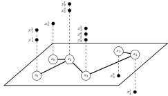
Figure 1: Example of graph $\mathcal{G}^{\texttt{cmm}}$ and its related observations $\bm{\mathrm{x}}$.

For notational purpose, we introduce the following shorthands:

$$\begin{split}\bm{x}_{i}&=(x_{i}^{1},\dots,x_{i}^{L_{i}})^{\top},\quad\\ \theta_{i}&=\theta(s_{i}),\end{split}\quad\begin{split}\bm{\mathrm{x}}&=(\bm{x}_{1}^{\top},\dots,\bm{x}_{N}^{\top})^{\top},\\ \bm{\theta}&=(\theta_{1},\dots,\theta_{N})^{\top}.\end{split}$$

From the observation model (1) and the assumption that noises are i.i.d. Gaussian variables, it follows that

$$p(\bm{\mathrm{x}}|\bm{\theta}) =\prod_{i=1}^{N}p(\bm{x}_{i}|\theta_{i})=\prod_{i=1}^{N}\prod_{\ell=1}^{L_{i}}p(x_{i}^{\ell}|\theta_{i}),$$ (2a)

$$p(x_{i}^{\ell}|\theta_{i}) \sim\mathcal{N}(\theta_{i},\sigma^{2}).$$ (2b)

Given the observations $\bm{\mathrm{x}}$ and the graph $\mathcal{G}^{\texttt{cmm}}$, our goal is to design a distributed algorithm allowing nodes to estimate the value of the spatial field $\theta(\cdot)$ in a set of regression (or testing) points $s^{R}_{1},\dots,s^{R}_{M}\in P$.

It is worth noticing that the regression points can either coincide or not with the measurement points. In the first case, a node $i$ in the network is trying to improve its local estimate of $\theta(s_{i})$, while in the second one it wants to interpolate the field in a neighboring point where measurements are missing. In the following we will show how a single node can take advantage of all other measurements in the network by exchanging information only with neighboring nodes.

III Empirical Bayes Framework

In this section we introduce a probabilistic model allowing nodes, especially the ones with few measurements, to have a better estimate of the spatial field at their measurement points or in neighboring areas.

III-A Probabilistic Model

We adopt a Bayesian model in which the spatial field $\theta(\cdot)$ is a Gaussian Process with mean function $\mu(\cdot)$ and covariance function $K(\cdot,\cdot)$, denoted by

$$\theta(\cdot) \sim\mathcal{GP}(\mu(\cdot),K(\cdot,\cdot)).$$ (3)

For the covariance function $K(\cdot,\cdot)$, known kernel functions can be used as customary. As for the mean function $\mu(\cdot)$, different from existing works where it is assumed to be null, we consider a more general parametric model which is meant to capture some prior knowledge. Since it is not realistic to assume the model (hyper)parameters to be known by nodes in the network, we propose an approach, based on the Empirical Bayes paradigm, in which hyperparameters will be estimated from the data through Maximum Likelihood (ML). As we will show through two example scenarios, this framework can model both a set-up in which prior knowledge encodes some (deterministic) physical law (but with unknown values of the physical parameters), and a data-driven inference scenario in which an interpolating function is used.

Formally, we introduce an interaction graph, $\mathcal{G}^{\texttt{int}}=(\{1,\dots,N\},\mathcal{E}^{\texttt{int}})$, induced by the Gaussian Process. We denote $\mathcal{N}_{i}^{\texttt{int}}=\{j:(i,j)\in\mathcal{E}^{\texttt{int}}\}$ the set of neighbors of node $i$ in the interaction graph. Consistently, we let $\bm{s}_{\mathcal{N}_{i}^{\texttt{int}}}=\big{[}s_{j}\big{]}_{j\in\mathcal{N}_{i}^{\texttt{int}}}$ be the vector of measurement points which are neighbors of point $s_{i}$, and $\bm{\mu}_{\mathcal{N}_{i}^{\texttt{int}}}=\big{[}\mu(s_{j})\big{]}_{j\in\mathcal{N}_{i}^{\texttt{int}}}$ the vector of values of $\mu(\cdot)$ at those points.

We, thus, assume that

$$K(s_{i},s_{j})\neq 0\iff(i,j)\in\mathcal{E}^{\texttt{int}},$$ (4)

and that $\mu(\cdot)$ is the (unique) solution of the following parametrized system of equations, termed spatial dynamics:

$$F_{i}(\bm{s}_{\mathcal{N}_{i}^{\texttt{int}}},\bm{\mu}_{\mathcal{N}_{i}^{\texttt{int}}};\bm{\gamma})=0,\qquad i=1,\dots,N,$$ (5)

where the functions $F_{i}(\cdot,\cdot;\bm{\gamma})$ are known, while $\bm{\gamma}\in\Gamma$ is the unknown hyperparameter vector.

We point out that $\bm{\theta}$ is the vector of parameters of $\bm{\mathrm{x}}$, and $\bm{\gamma}$ is the parameter of $\bm{\theta}$, and thus the name hyperparameter.

III-B Examples of application scenarios

Here, we present two scenarios that highlight the flexibility of the proposed probabilistic framework. In the first one, we consider a set-up in which physical knowledge of the spatial field is available through a partial differential equation that can be discretized at the measurement points. In the second one, we show how interpolating curves can be used when there is no physical knowledge of the phenomenon.

III-B1 Temperature Dynamics

We consider a scenario in which sensors want to estimate the temperature in a given environment. In this case, the mean function $\mu(\cdot)$ of the spatial field $\theta(\cdot)$ is expected to obey the following Heat Equation parametrized by $\bm{\gamma}$:

$$\sum_{\ell=1}^{d}\!\partial^{2}_{\ell\ell}\mu(s,t)-\partial_{t}\mu(s,t)=w(s,t;\bm{\gamma}),$$

where $(s,t)\!\in\!P\!\times[0,T)$, $\partial_{\ell}$ is the partial derivative with respect to the $\ell$-th component of $s$, and $\partial_{t}$ is the partial derivative with respect to time $t$. The function $w(\cdot;\bm{\gamma})$ is also known as the heat source.

If one considers a thermostatic (equilibrium) condition, the Heat Equation turns out to be the so called Poisson Equation:

$$\sum_{\ell=1}^{d}\partial^{2}_{\ell\ell}\mu(s)=w(s;\bm{\gamma}),\quad s\in P\subset\mathbb{R}^{d}.$$

Now, in order to guarantee the uniqueness of $\mu(\cdot)$, we specify the boundary condition. For the sake of clarity, we consider the 1-dimensional case in which we want to monitor the temperature in a bar $P=[s_{1},s_{N}]$. As a consequence, $\mu(\cdot)$ is uniquely determined by the following Cauchy Problem

$$\begin{cases}\mu^{\prime\prime}(s)=w(s;\bm{\gamma}),&\quad s\in(s_{1},s_{N}),\\ \hskip 2.0pt\mu(s_{1})=w_{1},\\ \mu(s_{N})=w_{N}.\end{cases}$$

Then, the Poisson Equation can be discretized at the measurement points $s_{1},\dots,s_{N}$, by using a suitable approximation rule as, e.g.,

$$\mu(s_{i})^{\prime\prime}\approx\frac{\mu(s_{i+1})-2\mu(s_{i})+\mu(s_{i-1})}{\epsilon^{2}},\quad i=2,\dots,N-1,$$

where we have assumed, for simplicity, that the measurement points are uniformly spaced, i.e., $\epsilon\!=\!s_{i+1}-s_{i}$ for all $i\!=\!1,\dots,N-1$. By plugging in the boundary conditions, the discretized system turns out to be

$$\begin{bmatrix}1&&&&\\ 1&-2&1&&\\ &\ddots&\ddots&\ddots&\\ &&1&-2&1\\ &&&&1\end{bmatrix}\begin{bmatrix}\mu(s_{1})\\ \mu(s_{2})\\ \vdots\\ \mu(s_{N-1})\\ \mu(s_{N})\end{bmatrix}=\begin{bmatrix}w_{1}\\ \epsilon^{2}w(s_{2};\bm{\gamma})\\ \vdots\\ \epsilon^{2}w(s_{N-1};\bm{\gamma})\\ w_{N}\end{bmatrix},$$

which has the sparsity of (5) once we set

$$\mathcal{N}_{i}^{\texttt{int}} =\begin{cases}\{i\},&\text{for }i\in\{1,N\},\\ \{i-1,i,i+1\}&\text{otherwise},\end{cases}$$

and

$$F_{i}(\bm{s} {}_{\mathcal{N}_{i}^{\texttt{int}}},\bm{\mu}_{\mathcal{N}_{i}^{\texttt{int}}};\bm{\gamma})=$$

$$\begin{cases}\mu(s_{i})-u_{i},&\text{for }i\in\{1,N\},\\ \frac{\mu(s_{i+1})-2\mu(s_{i})+\mu(s_{i-1})}{\epsilon^{2}}-u(s_{i};\bm{\gamma})&\text{otherwise.}\end{cases}$$

We point out that, as depicted in Fig. 2, the discretization process may induce a set of neighbors, call it $\mathcal{N}_{i}^{\mu}$, while the covariance function may correlate with a broader set of agents, call it $\mathcal{N}_{i}^{K}\supset\mathcal{N}_{i}^{\mu}$. Clearly, we can set $\mathcal{N}_{i}^{\texttt{int}}=\mathcal{N}_{i}^{K}$.

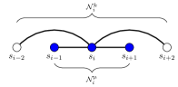
Figure 2: Neighborhoods of agent $i$ induced by the covariance function $K(\cdot,\cdot)$ and by the mean function $\mu(\cdot)$, denoted by $\mathcal{N}_{i}^{k}$ and $\mathcal{N}_{i}^{\mu}$ respectively.

III-B2 Interpolating Dynamics

Here we consider a data-driven inference scenario in which the shape of the mean $\mu(\cdot)$ is described by

$$\mu(s)=\mathcal{I}(s;\bm{\gamma}),\quad s\in P,$$

where $\mathcal{I}(s;\bm{\gamma})$ is an interpolation function (e.g., a cubic spline) of the points $\{(s_{i},\gamma_{i})\}_{i}$, parametrized by $\bm{\gamma}=(\gamma_{1},\dots,\gamma_{N})^{\top}\in\mathbb{R}^{N}$. This gives the possibility to fit the observations even if there is no information about the physics of the problem.

IV Distributed Empirical Bayes Estimator

In this section we develop our distributed estimation approach following the Empirical Bayes framework introduced in the previous section. Specifically, we derive the Maximum Likelihood (ML) estimator of the hyperparameter and the Maximum A Posteriori (MAP) estimator of the spatial field. Then, we show how to recast the ML problem into an equivalent optimization problem with a partitioned structure that is amenable to distributed computation. Finally, we provide a local procedure allowing each node to compute the MAP estimator of the field at its location or to perform a regression at nearby points.

We start by introducing some useful notation:

$$\begin{split}\mu_{i}&=\mu(s_{i}),\\ \mu^{R}_{m}&=\mu(s^{R}_{m}),\end{split}\qquad\begin{split}\bm{\mu}&=(\mu_{1},\dots,\mu_{N})^{\top},\\ \bm{\mu}^{R}&=(\mu^{R}_{1},\dots,\mu^{R}_{M})^{\top}.\end{split}$$

When needed, we highlight the dependence of $\bm{\mu}$ and $\bm{\mu}^{R}$ on $\bm{\gamma}$ (from (5)) by writing $\bm{\mu}_{\bm{\gamma}}$ and $\bm{\mu}^{R}_{\bm{\gamma}}$ respectively. Moreover, we define the matrices $K_{ss}\in\mathbb{R}^{N\!\times\!N}$ with entries $[K_{ss}]_{ij}\!=K(s_{i},s_{j})$, $K_{s^{R}s}\in\mathbb{R}^{M\!\times\!N}$ with entries $[K_{s^{R}s}]_{mi}\!=K(s^{R}_{m},s_{i})$, and consistently $K_{ss^{R}}$ and $K_{s^{R}s^{R}}$. We also introduce

$$\overline{x}_{i}=\frac{1}{L_{i}}\sum_{\ell=1}^{L_{i}}x_{i}^{\ell},\qquad \overline{\bm{\mathrm{x}}}=(\overline{x}_{1},\dots,\overline{x}_{N})^{\top}.$$

Finally,

$$[D]_{ij}=\delta_{ij} \frac{\sigma^{2}}{L_{i}}\in\mathbb{R}^{N\times N},$$

where $\delta_{ij}$ is the Kronecker delta (i.e., $\delta_{ij}=1$ for $i=j$ and $\delta_{ij}=0$ otherwise).

IV-A Distributed ML Estimator

The ML hyperparameter estimator is given by

$$\bm{\gamma}_{\textnormal{ML}}=\operatorname*{argmax}_{\bm{\gamma}\in\Gamma}p(\bm{\mathrm{x}};\bm{\gamma}).$$ (6)

We are now ready to state the first result characterizing the structure of optimization problem (6).

Theorem IV.1

The ML hyperparameter estimator $\bm{\gamma}_{\textnormal{ML}}$ in (6) can be equivalently obtained by solving the following minimization problem

$$\min_{\bm{\gamma}\in\Gamma}\;(\bm{\mu}_{\bm{\gamma}}-\overline{\bm{\mathrm{x}}})^{\top}(K_{ss}+D)^{-1}(\bm{\mu}_{\bm{\gamma}}-\overline{\bm{\mathrm{x}}}).$$ (7)

$\square$

The proof will be provided in a forthcoming document.

Next, we introduce the distributed formulation of the optimization problem (6). We start by observing that the most important consequence of (4) is that matrix $K_{ss}$ has the same sparsity as graph $\mathcal{G}^{\texttt{int}}$ and so does $K_{ss}+D$. However, looking at equation (7), we notice that $(K_{ss}+D)^{-1}$ is not necessarily a sparse matrix. In order to preserve the sparsity for a distributed computation, we then introduce a new optimization variable $\bm{z}$, so that $\bm{\gamma}_{\textnormal{ML}}$ can be computed by solving the following optimization problem:

$$\begin{split}\min_{\bm{\gamma}\in\Gamma,\bm{z}\in\mathbb{R}^{N}}\quad&\bm{z}^{\top}(K_{ss}+D)\bm{z},\\ \operatorname*{subj.to}\quad&(K_{ss}+D)\bm{z}=\bm{\mu}_{\bm{\gamma}}-\overline{\bm{\mathrm{x}}}.\end{split}$$ (8)

At this point, making explicit the relationship between $\bm{\mu}$ and $\bm{\gamma}$ due to (5), we can write (8) as

$$\begin{split}\min_{\bm{\gamma}\in\Gamma,\bm{z},\bm{\mu}\in\mathbb{R}^{N}}\quad&\bm{z}^{\top}(K_{ss}+D)\bm{z},\\ \operatorname*{subj.to}\quad&(K_{ss}+D)\bm{z}=\bm{\mu}-\overline{\bm{\mathrm{x}}},\\ \quad&F_{i}(\bm{s}_{\mathcal{N}_{i}^{\texttt{int}}},\bm{\mu}_{\mathcal{N}_{i}^{\texttt{int}}};\bm{\gamma})=0,\quad i=1,\dots,N.\end{split}$$ (9)

Defining the functions

$$f_{i}(\bm{z}_{\mathcal{N}_{i}^{\texttt{int}}}) =\frac{\sigma^{2}}{L_{i}}z_{i}^{2}+\sum_{j\in\mathcal{N}_{i}^{\texttt{int}}}z_{i}K(s_{i},s_{j})z_{j},\quad i=1,\dots,N,$$

$$g_{i}(\bm{z}_{\mathcal{N}_{i}^{\texttt{int}}}) =\frac{\sigma^{2}}{L_{i}}z_{i}+\overline{x}_{i}+\sum_{j\in\mathcal{N}_{i}^{\texttt{int}}}K(s_{i},s_{j})z_{j},\quad i=1,\dots,N.$$

we can rewrite (9) as

$$\begin{split}\min_{\bm{\gamma}\in\Gamma,\bm{z},\bm{\mu}\in\mathbb{R}^{N}}\;\,&\sum_{i=1}^{N}f_{i}(\bm{z}_{\mathcal{N}_{i}^{\texttt{int}}}),\\ \operatorname*{subj.to}\;\,&g_{i}(\bm{z}_{\mathcal{N}_{i}^{\texttt{int}}})=\mu_{i},\\ \;\,&F_{i}(\bm{s}_{\mathcal{N}_{i}^{\texttt{int}}},\bm{\mu}_{\mathcal{N}_{i}^{\texttt{int}}};\bm{\gamma})=0,\;i=1,\dots,N.\end{split}$$ (10)

which is a formulation of problem (7) amenable to distributed solution.

Due to this formulation, the solution $(\bm{\gamma}_{\textnormal{ML}},\bm{z}_{\bm{\gamma}_{\textnormal{ML}}},\bm{\mu}_{\bm{\gamma}_{\textnormal{ML}}})$ of (9) can be computed by solving an optimization problem that has a separable cost (i.e., the sum of $N$ local costs). Available distributed optimization algorithms can be adopted to this aim, e.g., [18], [19], [20]. The special sparsity of cost function and constraints could be exploited by using techniques as the one proposed in [21].

Remark IV.2

A special case is the one in which we have

$$F_{i}(\bm{s}_{\mathcal{N}_{i}^{\texttt{int}}},\bm{\mu}_{\mathcal{N}_{i}^{\texttt{int}}};\bm{\gamma})=F_{i}(\bm{s}_{\mathcal{N}_{i}^{\texttt{int}}},\mu_{i};\bm{\gamma}),\quad i=1,\dots,N.$$

In this case, if we define the functions

$$G_{i}(\bm{z}_{\mathcal{N}_{i}^{\texttt{int}}};\bm{\gamma})=F_{i}(\bm{s}_{\mathcal{N}_{i}^{\texttt{int}}},g_{i}(\bm{z}_{\mathcal{N}_{i}^{\texttt{int}}});\bm{\gamma}),\qquad i=1,\dots,N,$$

$\bm{\gamma}_{\textnormal{ML}}$ can be computed by solving the optimization problem:

$$\begin{split}\min_{\bm{\gamma}\in\Gamma,\bm{z}\in\mathbb{R}^{N}}\quad&\sum_{i=1}^{N}f_{i}(\bm{z}_{\mathcal{N}_{i}^{\texttt{int}}}),\\ \operatorname*{subj.to}\quad&G_{i}(\bm{z}_{\mathcal{N}_{i}^{\texttt{int}}};\bm{\gamma})=0,\quad i=1,\dots,N,\end{split}$$ (11)

which has a simpler structure that can be exploited to speed up the calculation. Moreover, when $\mu(\cdot)$ is an explicit function of $\bm{\gamma}$, i.e., $\mu(\cdot)=\mu(\cdot;\bm{\gamma})$, the constraints in (11) simplify as $G_{i}(\bm{z}_{\mathcal{N}_{i}^{\texttt{int}}};\bm{\gamma})=g_{i}(\bm{z}_{\mathcal{N}_{i}^{\texttt{int}}})-\mu(s_{i};\bm{\gamma})$. $\square$

The vector $\bm{\mu}_{\bm{\gamma}_{\textnormal{ML}}}$ gives the evaluation of the Gaussian Process mean $\mu(\cdot)$ in the measurement points. Once a value of $\bm{\gamma}_{\textnormal{ML}}$ is available, computing nodes located at the measurement points may interpolate $\mu(\cdot)$ at regression points $s^{R}_{m}$ in their spatial proximity, i.e., $\big{[}\bm{\mu}^{R}_{\bm{\gamma}_{\textnormal{ML}}}]_{m}$, as follows.

• If $\mu(\cdot)$ satisfies a (discretized) partial differential equation parametrized by $\bm{\gamma}$, then $\big{[}\bm{\mu}^{R}_{\bm{\gamma}_{\textnormal{ML}}}]_{m}$ can be obtained by integrating the differential equation with hyperparameter $\bm{\gamma}_{\textnormal{ML}}$ and suitable boundary conditions based on neighboring points in the interaction graph.

• If $\mu(\cdot)$ is an explicit function of $\bm{\gamma}$, then $\big{[}\bm{\mu}^{R}_{\bm{\gamma}_{\textnormal{ML}}}]_{m}$ can be obtained by $\big{[}\bm{\mu}^{R}_{\bm{\gamma}_{\textnormal{ML}}}]_{m}=\mu(s^{R}_{m};\bm{\gamma}_{\textnormal{ML}})$.

• Alternatively, an interpolation can be performed by using the set of neighboring points.

IV-B Local MAP Estimator

In this subsection we show how a node can locally compute the MAP estimator $\bm{\theta}^{R}_{\textnormal{MAP}}$. Defining $\theta^{R}_{i}=\theta(s^{R}_{i})$ and $\bm{\theta}^{R}=(\theta^{R}_{1},\dots,\theta^{R}_{M})^{\top}$, the MAP estimator in the regression points is given by

$$\bm{\theta}^{R}_{\textnormal{MAP}}=\operatorname*{argmax}_{\bm{\theta}^{R}\in X^{M}\subset\mathbb{R}^{M}}p(\bm{\theta}^{R}|\bm{\mathrm{x}};\bm{\gamma}_{\textnormal{ML}}).$$ (12)

Notice that, once a value for $\bm{\gamma}_{\textnormal{ML}}$ is available, the estimation proceeds similarly as in a purely Bayesian set-up, where the prior distribution is fully specified and given by $\mathcal{N}(\bm{\mu}^{R}_{\bm{\gamma}_{\textnormal{ML}}},K_{s^{R}s^{R}})$. Specifically, the case in which the prior is known and each sensor $i$ performs only one observation ($L_{i}=1$) has been widely investigated in the literature [1].

In our work we generalize this classical framework in two ways. First, we consider a heterogeneous network set-up in which nodes perform a different number of observations, so that even those with few observations take advantage of nodes with more observations (especially neighboring ones). Second, this MAP estimator exploits the ML estimation of the hyperparameters, thus “optimally” adapting the prior to all network data. In the next theorem we provide a closed form expression of the posterior distribution, and, based on that, we derive a formulation of the MAP estimator which can be computed by each node in the network in a decentralized way (i.e., by collecting data from neighboring nodes in the interaction graph).

Theorem IV.3

The posterior distribution $p(\bm{\theta}^{R}|\bm{\mathrm{x}};\bm{\gamma}_{\textnormal{ML}})$ is a multivariate Gaussian with mean $\bm{\mu}^{R}_{\bm{\gamma}_{\textnormal{ML}}}-K_{s^{R}s}\bm{z}_{\bm{\gamma}_{\textnormal{ML}}}$, where $\bm{z}_{\bm{\gamma}_{\textnormal{ML}}}$ is a solution of problem (10), and covariance matrix $K_{s^{R}s^{R}}-K_{s^{R}s}(K_{ss}+D)^{-1}K_{ss^{R}}$. Moreover, by defining $\mathcal{N}_{m}^{E}:=\{j:K(s^{R}_{m},s_{j})\neq 0\}$, the MAP estimator at $s^{R}_{m}$ is given by

$$\big{[}\bm{\theta}^{R}_{\textnormal{MAP}}\big{]}_{m} =\big{[}\bm{\mu}^{R}_{\bm{\gamma}_{\textnormal{ML}}}]_{m}-\sum_{j\in\mathcal{N}_{m}^{E}}K(s^{R}_{m},s_{j})\big{[}\bm{z}_{\bm{\gamma}_{\textnormal{ML}}}\big{]}_{j}. \square$$

The proof will be provided in a forthcoming document.

It is worth noting that if a regression point coincides with a measurement point, i.e., $s^{R}_{m}=s_{m}$, then $\mathcal{N}_{m}^{E}=\mathcal{N}_{i}^{\texttt{int}}$ and

$$\big{[}\bm{\theta}^{R}_{\textnormal{MAP}}\big{]}_{i}=\big{[}\bm{\mu}_{\bm{\gamma}_{\textnormal{ML}}}\big{]}_{i}-\sum_{j\in\mathcal{N}_{i}^{\texttt{int}}}\big{[}K_{ss}\big{]}_{ij}\big{[}\bm{z}_{\bm{\gamma}_{\textnormal{ML}}}\big{]}_{j}.$$

For a regression point $s^{R}_{m}$ that does not coincide with a measurement point, a computing node located at $s^{R}_{m}$, or equivalently one of the network nodes in the proximity, can obtain $\big{[}\bm{\mu}^{R}_{\bm{\gamma}_{\textnormal{ML}}}]_{m}$ through the interpolation procedure described in the previous subsection, and collect $\big{[}\bm{z}_{\bm{\gamma}_{\textnormal{ML}}}\big{]}_{j}$ from $j\in\mathcal{N}_{m}^{E}$. Notice that the sparsity of the kernel with respect to the entire space $P$ implies that $\mathcal{N}_{m}^{E}$ typically contains a limited number of nodes.

Generally speaking, Theorem IV.3 provides an efficient way to compute the MAP estimator at each point. In fact, if one used the standard formula of the posterior (see [1]) the MAP estimator would be $\bm{\mu}^{R}_{\bm{\gamma}_{\textnormal{ML}}}-K_{s^{R}q}(K_{qq}+\sigma^{2}I_{L})^{-1}(\bm{\mu}_{L}-\bm{\mathrm{x}})$ where $L=\sum_{i=1}^{N}L_{i}$, $q=(\underbrace{s_{1},\ldots,s_{1}}_{L_{1}},\ldots,\underbrace{s_{N},\ldots,s_{N}}_{L_{N}})^{\top}$ and $\bm{\mu}_{L}=(\underbrace{\mu(s_{1}),\ldots,\mu(s_{1})}_{L_{1}},\ldots,\underbrace{\mu(s_{N}),\ldots,\mu(s_{N})}_{L_{N}})^{\top}$, thus involving matrices of much larger size.

V Numerical Simulations

In this section we analyze the numerical results related to the two example scenarios introduced in Section III-B. We have used, in both cases, a kernel function known as Mahalanobis function (see [22]), which allows us to make $K_{ss}$ sparse. Moreover, we took as regression points a fine grained discretization of the (one dimensional) set $P$ to better visualize the regression in the entire spatial domain.

V-A Temperature Dynamics

For this numerical simulation, we have considered $N=10$ sensors uniformly spaced between $s_{1}=0$ and $s_{N}=2\pi/3$. The vector $\bm{\mathrm{x}}$ of observations has been generated according to the following Temperature dynamics,

$$\begin{cases}\mu^{\prime\prime}(s)=-A\omega^{2}\sin(\omega s+\phi),&\quad s\in(s_{1},s_{N}),\\ \hskip 2.0pt\mu(s_{1})=w_{1},\\ \mu(s_{N})=w_{N}.\end{cases}$$

where the right hand side of the first equation represents the heat source with $A=6$, $\omega=3$ and $\phi=3$, and the boundary conditions are $w_{1}=3$ and $w_{N}=0$.

This differential equation has a closed form solution $\theta(s)=A\sin(\omega s+\phi)+C_{1}s+C_{0}$, with

$$C_{1} :=\frac{w_{N}+A\sin(\omega s_{N}+\phi)-w_{1}-A\sin(\omega s_{1}+\phi)}{s_{N}-s_{1}},$$

$$C_{0} :=w_{1}-A\sin(\omega s_{1}+\phi)-C_{1}s_{1},$$

so that the $\ell$-th observation at $s_{i}$ is given by $x_{i}^{\ell}=\theta(s_{i})+\epsilon_{i}$.

In the estimation process we assume that the prior available information is the above family of Temperature dynamics with parameters $\bm{\gamma}=(A,\omega,\phi)^{\top}$ being the hyperparameters of our framework. Once $\bm{\gamma}_{\textnormal{ML}}$ has been obtained, $\bm{\mu}^{R}_{\bm{\gamma}_{\textnormal{ML}}}$ can be computed by integrating the Cauchy problem.

The result of the simulation is depicted in Fig. 3, where the estimated (process) prior mean in the regression points, $\bm{\mu}^{R}_{\bm{\gamma}_{\textnormal{ML}}}$, is depicted in blue, the posterior mean $\bm{\theta}^{R}_{\text{MAP}}$ is shown in green and the true field $\theta(\cdot)$ in red. Remarkably, both the $\bm{\mu}^{R}_{\bm{\gamma}_{\textnormal{ML}}}$ and $\bm{\theta}^{R}_{\text{MAP}}$ provide an accurate estimate of the spatial field $\theta(\cdot)$. As one would expect, at measurement points with a greater number of observations the local estimation is more accurate with a tighter confidence bound.

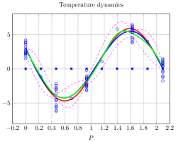
Figure 3: Temperature dynamics scenario: the measurement points $s_{i}$ are marked with a cross, while the observations $\bm{\mathrm{x}}$ with circles. The red line is the true mean function $\mu(\cdot)$, the blue line is $\bm{\mu}^{R}_{\bm{\gamma}_{\textnormal{ML}}}$ and the green line is the posterior mean $\bm{\theta}^{R}_{\text{MAP}}$. In magenta we represent the 95% confidence bound for the posterior mean.

V-B Interpolating Dynamics

In this case we have considered $N=12$ sensors spaced non-uniformly between $s_{1}=-15$ and $s_{N}=14$. The vector $\bm{\mathrm{x}}$ of observations has been generated according to a spatial field $\theta(\cdot)$ being a quadratic polynomial, i.e.,

$$\theta(s)=as^{2}+bs+c,$$ (13)

where we have chosen $a=0.1$, $b=0.1$ and $c=10$.

Differently from the previous numerical example, during the estimation process we have used as parametrized mean function (prior) an interpolating curve that does not match (13). In fact we have used the family of natural cubic splines. Specifically, we have taken $N=12$ measurement points $s_{1},\ldots,s_{12}$ clustered in five subregions. Then we have chosen as control points $c_{j}$ of the spline one point for each cluster, namely $c_{1}=s_{1}$, $c_{2}=s_{3}$, $c_{3}=s_{5}$, $c_{4}=s_{7}$ and $c_{5}=s_{12}$.

Specifically, the spline function is defined as

$$\mu(s)=\begin{cases}p_{1}(s),&\mbox{ if }s<c_{1},\\ p_{j}(s),&\mbox{ if }s\in[c_{j},c_{j+1}),\\ p_{N-1}(s),&\mbox{ if }s\geq c_{5},\end{cases}$$

where each cubic polynomial $p_{j}(\cdot)$ satisfies the following conditions:

$$\begin{cases}p_{j}(c_{j})=\gamma_{j},\quad p_{j}(c_{j+1})=\gamma_{j+1},&j=1,\dots,4,\\ p_{j-1}^{\prime}(c_{j})=p_{j}^{\prime}(c_{j}),&j=2,\dots,4,\\ p_{j-1}^{\prime\prime}(c_{j})=p_{j}^{\prime\prime}(c_{j}),&j=2,\dots,4\\ p_{1}^{\prime\prime}(c_{1})=0,\quad p_{4}^{\prime\prime}(c_{5})=0,\end{cases}$$

with $\bm{\gamma}=(\gamma_{1},\ldots,\gamma_{5})^{T}$.

The result of the simulation is depicted in Fig. 4. As in the previous example, the estimate is more accurate in those points with an higher number of observations. Moreover, we can appreciate the capability of the Interpolating dynamics of fitting the spatial field $\theta(\cdot)$ near the measurement points.

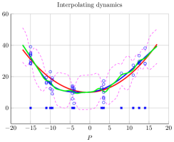
Figure 4: Interpolating dynamics scenario: the measurament points $s_{i}$ are labeled with a cross, while the observations $\bm{\mathrm{x}}$ are marked with circles. The red line is the true mean function $\mu(\cdot)$, the blue line is $\bm{\mu}^{R}_{\bm{\gamma}_{\textnormal{ML}}}$ and the green line is the posterior mean $\bm{\theta}^{R}_{\text{MAP}}$. In magenta we represent the 95% confidence interval relative to the posterior mean.

VI Conclusions

In this paper we have proposed a novel probabilistic framework for distributed estimation of a spatial field in large-scale sensor networks, wherein each node performs multiple, local measurements. The proposed set-up is based on an Empirical Bayes approach in which the spatial field is modeled as a Gaussian Process with known covariance and unknown, but parametrized, mean. Specifically, we suppose that the mean function at the measurement points satisfies a set of equations (encoding some prior knowledge of the mean shape) parametrized by the unknown hyperparameters. The Empirical Bayes estimation procedure consists of two parts: the computation of the ML estimate of the hyperparameters, and the computation of the MAP estimate of the field into regression points. In particular, we have shown that multiple observations improve the estimation accuracy by reducing the posterior variance, and we have also provided a sparse formulation of the ML optimization problem, which is amenable to distributed solution. Thus, each sensor optimally fuses information from the network in a distributed way thus improving its own MAP estimate of the field. Numerical simulations for the proposed scheme have been presented for two example scenarios. In the first one, the temperature field in a thermostatic bar is estimated by using the Heat Equation as a prior knowledge for the mean. In the second one, interpolating curves have been used in a data-driven inference scenario with no physical knowledge of the field.

References

• [1] C. E. Rasmussen and C. K. Williams, Gaussian processes for machine learning.   MIT press Cambridge, 2006, vol. 1.
• [2] A. Carron, M. Todescato, R. Carli, L. Schenato, and G. Pillonetto, “Machine learning meets Kalman filtering,” in IEEE 55th Conference on Decision and Control (CDC), 2016, pp. 4594–4599.
• [3] M. Todescato, A. Dalla Libera, R. Carli, G. Pillonetto, and L. Schenato, “Distributed Kalman filtering for time-space Gaussian processes,” IFAC Proceedings Volumes, 2017.
• [4] Y. Xu, J. Choi, S. Dass, and T. Maiti, “Bayesian prediction and adaptive sampling algorithms for mobile sensor networks,” in IEEE American Control Conference (ACC), 2011, pp. 4195–4200.
• [5] N. Cressie, Statistics for spatial data.   John Wiley & Sons, 2015.
• [6] M. L. Stein, Interpolation of spatial data: some theory for Kriging.   Springer Science & Business Media, 2012.
• [7] J. Cortés, “Distributed kriged Kalman filter for spatial estimation,” IEEE Transactions on Automatic Control, vol. 54, no. 12, pp. 2816–2827, 2009.
• [8] S. Martinez, “Distributed interpolation schemes for field estimation by mobile sensor networks,” IEEE Transactions on Control Systems Technology, vol. 18, no. 2, pp. 491–500, 2010.
• [9] D. Varagnolo, G. Pillonetto, and L. Schenato, “Distributed parametric and nonparametric regression with on-line performance bounds computation,” Automatica, vol. 48, no. 10, pp. 2468–2481, 2012.
• [10] A. Kozma, J. Andersson, C. Savorgnan, and M. Diehl, “Distributed multiple shooting for optimal control of large interconnected systems,” IFAC Proceedings Volumes, vol. 45, no. 15, pp. 143–147, 2012.
• [11] D. Georges, “Optimal sensor location and mobile sensor crowd modeling for environmental monitoring,” IFAC Proceedings Volumes, 2017.
• [12] M. L. Elwin, R. A. Freeman, and K. M. Lynch, “Environmental estimation with distributed finite element agents,” in IEEE 55th Conference on Decision and Control (CDC), 2016, pp. 5918–5924.
• [13] R. Graham and J. Cortés, “Spatial statistics and distributed estimation by robotic sensor networks,” in IEEE American Control Conference (ACC), 2010, pp. 2422–2427.
• [14] J. Le Ny and G. J. Pappas, “On trajectory optimization for active sensing in Gaussian process models,” in 48th IEEE Conference on Decision and Control held jointly with the 28th Chinese Control Conference. CDC/CCC, 2009, pp. 6286–6292.
• [15] B. M. Bell and G. Pillonetto, “A distributed Kalman smoother,” IFAC Proceedings Volumes, vol. 42, no. 20, pp. 132–137, 2009.
• [16] A. Coluccia and G. Notarstefano, “Distributed estimation of binary event probabilities via hierarchical Bayes and dual decomposition,” in IEEE 52nd Conference on Decision and Control (CDC), 2013, pp. 6753–6758.
• [17] A. Coluccia and G. Notarstefano, “A Bayesian framework for distributed estimation of arrival rates in asynchronous networks,” IEEE Transactions on Signal Processing, vol. 64, no. 15, pp. 3984–3996, 2016.
• [18] R. Carli, G. Notarstefano, L. Schenato, and D. Varagnolo, “Analysis of Newton-Raphson consensus for multi-agent convex optimization under asynchronous and lossy communications,” in 54th IEEE Conference on Decision and Control, 2015, pp. 418–424.
• [19] A. Nedić and A. Olshevsky, “Distributed optimization over time-varying directed graphs,” IEEE Transactions on Automatic Control, vol. 60, no. 3, pp. 601–615, 2015.
• [20] Y. Sun, G. Scutari, and D. Palomar, “Distributed nonconvex multiagent optimization over time-varying networks,” in IEEE 50th Asilomar Conference on Signals, Systems and Computers, 2016, pp. 788–794.
• [21] R. Carli and G. Notarstefano, “Distributed partition-based optimization via dual decomposition,” in IEEE 52nd Conference on Decision and Control (CDC), 2013, pp. 2979–2984.
• [22] A. Melkumyan and F. Ramos, “A sparse covariance function for exact Gaussian process inference in large datasets,” in 21st international jont conference on Artifical intelligence.   Morgan Kaufmann Publishers Inc., 2009, pp. 1936–1942.