Separation of conditions as a prerequisite for quantum theory

Abstract

We introduce the notion of “separation of conditions” meaning that a description of statistical data obtained from experiments, performed under a set of different conditions, allows for a decomposition such that each partial description depends on mutually exclusive subsets of these conditions. Descriptions that allow a separation of conditions are shown to entail the basic mathematical framework of quantum theory. The Stern-Gerlach and the Einstein-Podolsky-Rosen-Bohm experiment with three, respectively nine possible outcomes are used to illustrate how the separation of conditions can be used to construct their quantum theoretical descriptions. It is shown that the mathematical structure of separated descriptions implies that, under certain restrictions, the time evolution of the data can be described by the von Neumann/Schrödinger equation.

I Introduction

Most of us heavily rely on our visual system to perform tasks in daily life. The ability of our visual system to rapidly and effortlessly decompose a visual scene into separate objects and categorize them according to their functionality considerably enhances the chance of survival of the individual. The example of the visual system is just one of the many instances in which our cognitive system constantly performs separations “on the fly”. In daily life, we hardly notice that our brains are performing these separations, suggesting that the basic processes involved are, as a result of evolution, hardwired into our brains. Therefore, it is not a surprise that in many forms of cognitive activity, also in the most abstract modes of human reasoning, separation into parts plays an important role.

There is a large variety problems in mathematics and physics for which separation into parts is of great value. For instance, separation of variables is a very powerful method for solving (partial) differential equations. Describing the harmonic vibrations in solids in terms of normal modes (phonons) instead of using the displacements of the atoms and their momenta is much more effective for understanding their properties. Analyzing a signal in terms of Fourier components is a standard method for decomposing the signal into a sum of signals that each have a simple description. Similarly, computing the principal components of a correlation matrix yields a description of the data that, in many cases, is considerably simpler than the description of the data themselves.

The ubiquity of separation in cognitive processes suggests that it may be an important guiding principle for developing useful descriptions of the phenomena that we observe. In this paper, this guiding principle is used for the analysis and representation of data, as expressed by the statement

The separation of conditions (SOC), when applied to data produced by experiments performed under several different sets of conditions (e.g. $\{(a,b),(a^{\prime},b^{\prime})\}$), reduces the complexity of describing the collective of these experiments by decomposing the description of the whole into descriptions of several parts which depend on mutually exclusive, proper subsets (e.g. $\{(a),(a^{\prime})\}$ and $\{(b),(b^{\prime})\}$) of the conditions only.

It is important to recognize that SOC operates on a much more primitive level than e.g. the principle of stationary action which is central in modern theoretical physics. SOC serves as the foundation for a chain of reasoning whereas the principle of stationary action refers to a general variational method that has numerous applications across a wide field. The latter principle is used to derive equations of motion from a postulated functional called “action” whereas SOC is used by our cognitive system for a variety of functions.

It is remarkable that the evolution of our physical worldview goes hand in hand with evolution of the main mathematical tools of theoretical physics. Classical mechanics is based on the concept of materials points and enforces the use of ordinary differential equations Newton (1999). According to Arnold Arnold (1990), the main achievement and the main idea of Newton can be formulated in one sentence: “It is useful to solve (ordinary) differential equations”. The Faraday-Maxwell revolution of 19th century placed the concept of field in the center of theoretical physics, the corresponding mathematical apparatus being partial differential equations Einstein and Infeld (1967). Both the concepts of materials points and fields (e.g. water waves) relate directly to our daily experience Weyl (1994). In contrast, in quantum theory, “states” of a system are vectors in a Hilbert space, “observables” are Hermitian operators, and the mathematical apparatus is linear algebra and functional analysis von Neumann (1955). None of these concepts directly relates to elements of an experiment. Numerous works on “interpretation of quantum theory” – for a brief or concise overview of popular interpretations see Ref. Weinberg, 2003 or Ref. Rauch and Werner, 2015, respectively – offer tens, hundreds of ways how to interpret the symbols of this language; much less is known about its origin. Why is it that such abstract concepts play the central role in our description of microscopic phenomena? In this paper, we present an attempt to clarify this issue based on a careful analysis of ways to organize information (represented by “experimental data”) and of ways to operate with it.

The view adopted in this paper is that the primary goal of a theoretical model should be to provide concise descriptions of the available data which constitute the objective information (i.e., free of personal judgment), about the phenomena under scrutiny. In addition, it is desirable to construct such descriptions using mathematics that is as simple as possible. Due to the general, non-mathematical nature of SOC, it is impossible to deduce or derive, in the mathematical sense, the basic postulates of quantum theory from SOC only: one has to inject into the mathematical framework that is constructed on the basis of SOC, additional knowledge about the specific conditions under which the experiments are being performed. In this paper, we adopt the traditional approach of theoretical physics by assuming that the phenomena under scrutiny allow for a continuum space-time description. In other words, the additional assumption that we will use (implicitly) is that, in mathematical terms, the symmetries of the space-time continuum apply. Furthermore, as discussed later in this paper, quantum theory is not the only theory consistent with SOC, a statement which we will symbolically denote as

$$\mathrm{SOC}\models\mathrm{QT},$$ (1)

meaning that models in $\mathrm{SOC}$ entail models of $\mathrm{QT}$. However, the application of SOC yields a framework that is specific enough such that the language of operators and state vectors appears in a natural manner, consistent with our experience that experiments count individual events. Phrased more concisely, we show that quantum theory is a model for the specific class of data (of frequencies of events) to which SOC applies.

I.1 Quantum physics experiments

Consider a typical scattering experiment in which a crystal is targeted by neutrons produced by a nuclear reactor. Obviously, a description of the experiment as a whole is much too complicated to be useful. Therefore, we simplify matters. First, we leave out the description of the whole nuclear reactor as a neutron source and imagine a fictitious source preparing neutrons with well-defined momenta. Next, we assume that we know how to model the interaction of the neutrons with the atoms of the crystals. The measurement itself consists of detecting, one-by-one, the neutrons that leave the crystal in various directions. Finally, interpreting the counts of the neutrons scattered by the crystal in terms of the neutron-crystal interaction model allows us to make inferences about the lattice or magnetic structure of the crystal.

From this rough sketch of the neutron scattering experiment, it is clear that SOC has been used before any attempt is made to describe the experiment by a mathematical model. SOC seems to be an (implicit) assumption of all physical theories that have been invented. In particular, standard introductions of the quantum formalism assume – and do so often implicitly – that a model of the experiment can be decomposed into a preparation stage and a measurement stage, before the first postulate is introduced, see e.g. Ref. Ballentine (2003).

A characteristic feature of quantum physics experiments such as the neutron scattering experiment sketched earlier is the uncertainty in behavior of the individual neutrons. In essence, single events are regarded as irreproducible. Moreover, because the observed counts are the basis for making inferences about the interaction model, these inferences may be subject to additional uncertainties, in addition to those due to the uncertainties on the incoming neutrons. If single events are not reproducible, we may have (but not necessarily have) the situation that in the long run, the relative frequencies of the different detection events approach reproducible numbers. The latter means that upon repetition of the whole experiment, i.e. by collecting the data of many detection events, deviations of the new relative frequencies from the previous ones are within the statistical errors, e.g. they satisfy the law of large numbers Barlow (1989); Grimmet and Stirzaker (2001).

Results of laboratory experiments are always subject to uncertainties. In the theoretical description of these results we may choose to ignore these uncertainties, for good reason as in Newtonian mechanics, or not, as in quantum theory. The latter has no means by which to calculate the outcome of an individual event, a feature it shares with Kolmogorov’s probability theory Kolmogorov (1956); Grimmet and Stirzaker (2001). Not being able to deduce from a theory the very existence of the individual events that we observe is at the heart of the difficulties of understanding what the theory is about and what it describes.

I.2 Quantum theory

Quantum theory is probably the most obscure and impenetrable subject of all current scientific theories. Text books on quantum theory usually start with a brief historical account of the experiments that were crucial for the development of the theory to make plausible the postulates which define the mathematical framework Bohm (1951); Feynman et al. (1965); Ballentine (1970); Khrennikov (2009); Ballentine (2003). Subsequent efforts then go into mastering linear algebra in Hilbert space, solving partial differential equations, and other abstract mathematical tools. The tendency to focus on the elegant mathematical formalism von Neumann (1955), which, unfortunately, is far more detached from everyday experience than for instance Newtonian mechanics or electrodynamics, promotes the “shut-up-and-calculate” approach Ralston (2017). Hermitian operators, wave functions, and Hilbert spaces are conceptual, mental constructs which have no tangible counterpart in the world as we experience it through our senses. The mathematical results that are derived from the postulates of a theoretical model are only theorems within the axiomatic framework of that theoretical model. Theoretical physics uses axiomatic frameworks which have a rich mathematical structure, allowing the proof of theorems. For instance, the Banach-Tarsky paradox Banach and Tarski (1924) has no counterpart in the world that humans experience. Taking the mathematical description for real is like opening bottles that contain very exotic and sometimes magical substances. In other words, relating theorems derived within a mathematical axiomatic formalism to observable reality is not a trivial matter.

In quantum theory, the mapping from what occurs in Hilbert space to what is taking place in the laboratory is further convoluted by the fact that quantum theory lacks the means to account for the fact that a single measurement has a definite outcome Bohm (1951); Feynman et al. (1965); Ballentine (2003). That is, quantum theory cannot describe the fact that humans register individual events although it does a wonderful job to describe, under appropriate conditions, the frequencies with which these events occur. The conundrum of not being able to deduce from the theory that each measurement yields a definite outcome Allahverdyan et al. (2017) manifests itself in the number of different quantum-theory interpretations that exist today.

It may be of interest to mention here that the formalism of quantum theory finds applications in fields of science that are not even remotely related to the physics experiments which cannot be described by classical physics Khrennikov (2010). This begs the question “Why is the quantum formalism also useful in these non-quantum applications?”.

I.3 Application of SOC

In this paper, we explore a route, based on SOC, to construct the quantum theoretical description without running into the conundrum mentioned earlier. We start from the empirical fact that the result of a measurement yields a definite outcome. We review several different, simple ways to represent the moments of the relative frequencies of the different outcomes. It then follows that the mathematical structure underlying quantum theory is the simplest of many equivalent representations that allows the description of the experiment to be decomposed into a description of a preparation stage and a measurement stage (an implicit assumption in the formulation of quantum theory Ballentine (2003)).

It is obvious that this way of thinking is opposite to the more traditional, deductive reasoning which assumes an underlying ontology Bohm (1952); de la Peña and Cetto (1996); ’t Hooft (1997); de la Peña and Cetto (2005); ’t Hooft (2007) or starts from various, different sets of axioms Landé (1974); Frieden (1989); Vstovsky (1995); Reginatto (1998); Hardy (2001); Luo (2002); Frieden (2004); Bub (2007); Caves et al. (2007); Palge and Konrad (2008); Khrennikov (2009); Kapsa et al. (2010); Chiribella et al. (2011); Masanes and Müller (2011); Brukner (2011); Skála et al. (2011); Kapsa and Skála (2011); Oreshkov et al. (2012); Santamato and De Martini (2012); Klein (2010); Flego et al. (2012); Kapustin (2013); Fuchs and Schack (2013); Holik et al. (2014), the individual event being the last (but apparently unreachable) element in the chain of thoughts. This is also evident from the fact that in our construction there is no need to even mention the concept of probability, simply because the mathematical structure directly follows from a rearrangement of the data (counts of events) and the application of SOC. For a different approach based on rearranging data, see Ref. Ralston, 2013.

Another approach which reverses the chain of thought, i.e. starts from the notion of an individual event, uses the algebra of logical inference (LI), a mathematical framework for rational reasoning in the presence of uncertainty Cox (1946, 1961); Tribus (1999); Smith and Erickson (1989); Jaynes (2003). Applying LI to reproducible and robust experiments yields a description in terms of a seemingly complicated nonlinear global optimization problem, the solutions of which can be shown to be equivalent to the extrema of a quadratic form. For instance, for one particular scenario of collecting data, we recover the (time-dependent) Schrödinger equation De Raedt et al. (2014, 2016). Similary, for two other scenarios, LI yields the Pauli or Klein-Gordon equations, respectively, all without invoking concepts quantum theory De Raedt et al. (2015a); Donker et al. (2016).

The SOC approach only yields the basic mathematical framework, in essence only the postulates that appear in the statistical (ensemble) interpretation of quantum theory Ballentine (1970, 2003) (see below), knowledge about the specific physical problem has to be supplied in terms of symmetries, the correspondence principle etc., as in conventional quantum theory. In contrast, the LI approach starts from the notion of reproducible and robust frequencies of events, uses the requirement that in the absence of uncertainty classical Hamiltonian mechanics is recovered, and allows us to derive, in a strict mathematical sense, e.g. the Schrödinger equation of the hydrogen atom. So far, all equations derived on the basis of LI describe quantum systems in a pure state only De Raedt et al. (2013, 2014, 2015a, 2015b, 2016); Donker et al. (2016). Whether the LI approach can be extended to cover quantum systems in a mixed state is an open problem.

Recently, we have given simple examples, one of them in the context of the EPRB experiment, showing that LI can describe realizable data sets which do not allow for a quantum theoretical description De Raedt et al. (2018). Therefore, symbolically we have

$$\mathrm{LI}\models\mathrm{QT}^{\ast}.$$ (2)

where $\mathrm{QT}^{\ast}$ denotes the class of quantum systems characterized by pure states. On the other hand, the SOC approach contains the results of the LI approach, such that

$$\mathrm{SOC}\models\mathrm{LI}\models\mathrm{QT}^{\ast}\quad\mathrm{and}\quad\mathrm{SOC}\models\mathrm{QT}.$$ (3)

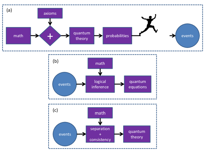
Figure 1: (Color online) Diagram illustrating the different chains of thought. (a) Traditional method to formulate quantum theory; (b) logical inference approach for deriving basic equations of quantum theory; (c) the approach explored in this paper. In contrast to the traditional method, which lacks the means to predict the individual, observable event, the other two approaches put the event at the core of reasoning. In (a) and (c) the box “quantum theory” refers to the mathematical framework, defined by postulates P1 and P2.

As already mentioned, this paper takes the notion of an individual event as the starting point but does not require the experiment to be reproducible nor to be robust. The only requirement is that the data gathered in one run is completely described by the relative frequencies of the different kinds of detection events, a number of which, in any laboratory experiment, is always finite. We show that SOC and consistency, combined with a simple reorganization of the observed data and some standard assumptions (e.g. symmetries of the space-time continuum ), are sufficient to construct the mathematical framework of quantum theory for a finite number of different outcomes. By consistency we mean that the description of a particular part is independent of the experiment or context in which the part is used.

A graphical representation of the traditional, the logical inference, and the SOC approach to introduce the formalism of quantum-theory is shown in Fig. 1. As far as we know, all interpretations of quantum theory are based on the same expressions for expectation values of dynamical variables such as position, energy etc. The difference between interpretations appears in the way the theoretical description deals with the measurement problem, i.e. “explains” that each measurement yields a definite outcome. The statistical (ensemble) interpretation of quantum theory is silent about this aspect. Copenhagen-like interpretations postulate the elusive wave function collapse to “explain” the existence of events.

Independent of the interpretation that one prefers, there is the crucial fact, almost never mentioned, that a genuine probabilistic theory does not entail a procedure or process by which elementary events can actually be produced. The existence of a set of elementary events is assumed, and probability theory is then built on this assumption Kolmogorov (1956). Ways to produce events according to a specified probability distribution would be (1) call Tyche to produce events without undiscoverable cause, i.e. appeal to magic, or (2) use an algorithm to let a computer generate events. Obviously, the latter is deterministic, pseudo-random in nature, does not produce random events in the strict mathematical sense, and is “outside” probability theory.

The two other approaches, graphically represented in Fig. 1(b,c), do not suffer from the problem of not being able to generate events. Indeed, in both the logical inference and the SOC approach, the event is the key element on which the whole theoretical structure is built. There is no need to have a procedure to generate events according to a specified probability distribution. Instead, this distribution is constructed from the frequencies of the events (and additional pieces of knowledge, depending on the case at hand).

Instead of discussing the application of SOC to quantum physics experiments in its most general form, we choose the more instructive route by demonstrating its application to two simple, but non-trivial experiments which have been instrumental in the development of quantum theory. The mathematical framework that emerges from applying SOC generalizes in an almost trivial manner. Following Feynman Feynman et al. (1965), we use the Stern-Gerlach (SG) experiment to illustrate how its quantum theoretical description directly emerges from a representation of the observed data in terms of independent, separate descriptions of the source and the SG magnet. We explicitly show that SOC in combination with the requirement of consistency and the use of symmetries of the space-time continuum suffice to recover the quantum theoretical description of a spin one ($S=1$) system. As a further illustration, we consider the Einstein-Podolsky-Rosen-Bohm experiment (EPRB) and show how also in this case the quantum theoretical description derives from a representation of the observed data in terms of independent, separate descriptions of the source and SG magnets. This example also demonstrates how to extend the approach to many-body problems. The work presented in this paper extends and generalizes our earlier work De Raedt et al. (2015b, 2016) on the spin-1/2 case.

I.4 Preview of the main result

In general terms, the main result of this paper can be summarized as follows. The mathematical structure of the following two postulates (or equivalent formulations of them)

P1. To each dynamical variable R (physical concept) there corresponds a linear operator $R$ (mathematical object), and the possible values of the dynamical variable are the eigenvalues of the operator Ballentine (2003).

and

P2. To each state there corresponds a unique state operator. The average value of a dynamical variable R, represented by the operator $R$, in the virtual ensemble of events that may result from a preparation procedure for the state, represented by the operator $\rho$, is $\langle R\rangle=\mathbf{Tr\;}\rho R/\mathbf{Tr\;}\rho$ Ballentine (2003).

which form the basis for the statistical (ensemble) interpretation of quantum theory Ballentine (1970, 2003) and suffice for all practical “shut-up-and-calculate” applications of quantum theory, directly follow from the application of SOC and a simple rearrangement of the data for the frequencies of the observed events. Note that neither quantum theory nor SOC yield the expressions of $\rho$ or $R$. Obviously, these expressions depend on the details of the experiment. Application of SOC to data gathered in quantum physics experiments provides an answer to the riddle “Where does the quantum formalism come from and why is it useful in non-quantum applications?”.

I.5 Structure of the paper

The paper is organized as follows. In Sec. II, we sketch the experimental setup of the double SG experiment that we use as the primary example to illustrate the application of SOC to data obtained by performing experiments under different conditions. Section III discusses the kind of data that are generated by this experiment and their characterization in terms of moments. In Sec. IV, we introduce SOC using the SG experiment with three different outcomes as an example and show that matrix algebra allows for the description to be separated in the sense of SOC. Explicit expressions for the description of the measurement stage are given in Secs. V and VI. The application to the double SG experiment, given in Sec. VII, completes the construction and also shows how the basic structure of the quantum formalism emerges from SOC. In Sec. VIII, we work out in detail a specific example of the double SG experiment and show that quantum theory restricts the functional dependence of the observed frequencies on the SG magnet parameters to those dependences for which separation is possible. Section IX discusses the most general description of the particle source and also the measurements that are required to fully characterize this source. Application of SOC enforces a representation of the data in terms of matrices, suggesting that there may be a relation to Heisenberg’s matrix mechanics Heisenberg (1925). In Sec. X, we scrutinize this relation and argue that if there is one, it is very weak. Section XI explores the conditions under which the time evolution of data that allows for a separated description can be described by the von Neumann/Schrödinger equation. Using the EPRB experiment as the simplest, nontrivial example, we demonstrate in Sec. XII how the tensor-product structure of quantum many-body physics naturally emerges from the application of SOC. In Sec. XIII, we discuss the general features of the SOC construction of the quantum formalism and its relation to the commonly accepted postulates of quantum theory. Our conclusions are given in Sec. XIV.

II Double Stern-Gerlach experiment

The SG experiment Gerlach and Stern (1922, 1924); Bohm (1951); Feynman et al. (1965) involves sending particles through an inhomogeneous magnetic field and observing their deflection. A source emits particles such as atoms Gerlach and Stern (1922, 1924), neutrons Sherwood et al. (1954); Hamelin et al. (1975), electrons Batelaan et al. (1997), or atomic clusters Diaz-Bachs et al. (2018). Particles are sent one-by-one through a SG magnet, the salient feature of which is that it generates an inhomogeneous magnetic field, along a direction characterized by the unit vector $\mathbf{a}$. The interaction of this field with magnetic moment of the particles changes the momentum of the latter. As a result, the particle beam is split into in $2S+1$ spatially well-separated directions which are determined by the unit vector $\mathbf{a}$, an experimental fact Gerlach and Stern (1922); Sherwood et al. (1954); Hamelin et al. (1975); Diaz-Bachs et al. (2018). This experimental fact is regarded as direct evidence for the quantized magnetic moment Gerlach and Stern (1922); Bohm (1951); Feynman et al. (1965). The latter is proportional to the “spin” of the particle and is assigned a magnitude $S$.

Assume that it is already established by experiments that there is a magnetic but no electric field between the poles of a SG magnet and that it is known, also from experiments, that the particles under scrutiny do not carry electrical charge. Then, if these particles pass through the SG magnet and show a deflection that is absent when the magnetic field is zero, it makes sense to assign the attribute “magnetic” to these particles. The observed deflection can be attributed to the interaction between the magnetic field inside the SG magnet and the assigned magnetic quality of the particles.

We now wish to go a step further and assign to the particles a definite magnetic moment, characterized by a direction and size, a necessary step if we want to speak about quantized magnetic moments.

In general, a consistent assignment of a particle property is a two-step process. First, we employ a filter to select particles. Then, using a second identical filter, we verify that all the particles pass that second filter. In the case at hand, this procedure amounts to performing a double SG experiment Bohm (1951); Feynman et al. (1965) such as the one sketched in Fig. 2. Only if the direction of the magnetic moment is “preserved” during repeated probing, it makes sense to attribute to the particle, a definite direction of magnetization.

We do not know of any laboratory realization of a double SG experiment but, following Feynman Feynman et al. (1965), we use this thought experiment to construct the theoretical description which, in contrast to Feynman’s approach, does not build on postulates of quantum theory. Also following Feynman Feynman et al. (1965), we focus on the case of particles which, in quantum parlance, are said to have spin $S=1$. Generalization to other values of the spin is straightforward Feynman et al. (1965). We emphasize that our choice to illustrate the main ideas by using experiments with three outcomes per SG magnet is only for the sake of balance between generality and simplicity. Our treatment readily generalizes to experiments with any number of different outcomes.

Following standard practice in developing theoretical models, we assume that the experiment is “perfect” in the sense that all SG magnets are identical, their inhomogeneous magnetic fields are constant for the duration of the experiment, each particle leaving the source is detected by one and only one of the nine detectors, and so forth.

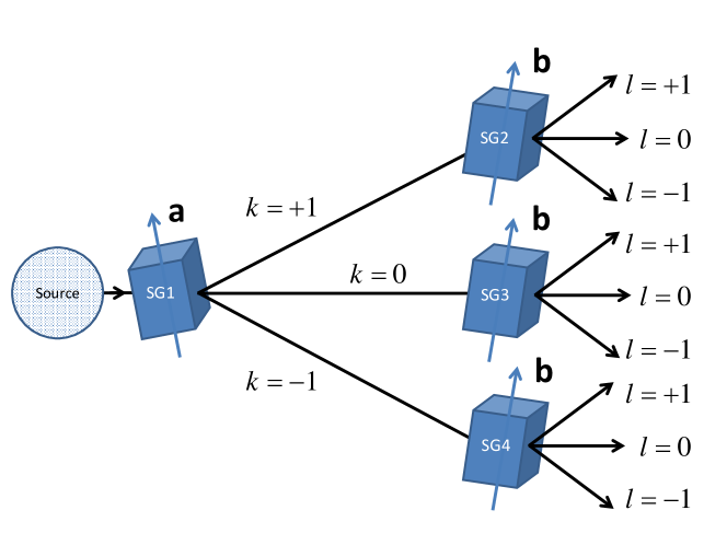
Figure 2: (Color online) Layout of the double Stern-Gerlach experiment that we consider in this paper. Electrically neutral, magnetic particles leave the source one-by-one and pass through the inhomogeneous magnetic field, characterized by the same unit vector $\mathbf{a}$, created by the Stern-Gerlach magnet SG1. Particles leave SG1 in one of the three beams labeled by $k=+1,0,-1$. The direction of these beams depends on the unit vector $\mathbf{a}$. Particles then travel to either SG2, SG3, or SG4, all three of them characterized by the same unit vector $\mathbf{b}$. Particles leave SG2, SG3, or SG4 in one of the three beams labeled by $l=+1,0,-1$. Finally, each particle is registered by one and only one detector (detectors not shown) labeled by $(k,l)$.

III Data generated by the experiment

As is clear from Fig. 2, for each particle leaving the source, one and only one detector, labeled by $(k,l)$, will fire. It may be tempting to say that the detected particle traveled along the beams labeled by $k$ and $l$ but as a matter of fact, on the basis of the available data, i.e. $(k,l)$, no such assignment can be made. On the other hand, for the purposes of this paper, it does no harm to imagine and it also simplifies the writing to say that the particle followed a particular path, but to know this for sure, we would have to add detectors in the beams between the SG1 and second layer of SG magnet.

We start by considering the experiment in which the second layer (SG2, SG3, SG4) is absent and detectors are placed in the beams labeled by $k$. We denote the counts of detector clicks recorded after $N$ particles have left the source by

$${\cal K}=\big{\{}k_{n}\;|\;k_{n}\in\{+1,0,-1\}\;;\;n=1,\ldots,N\big{\}}.$$ (4)

The relative frequency with which particles travel along the path $k$ is given by

$$f(k|\mathbf{a},P,N)=\frac{1}{N}\sum_{n=1}^{N}\delta_{k,k_{n}}.$$ (5)

We introduce the notation $|\mathbf{a},P,N)$ to indicate that the $N$ data items have been collected during a period in which $\mathbf{a}$ and the properties of the particles, represented by the symbol $P$, are assumed to be constant.

Similarly, for the double SG experiment, repeating the experiment with $N$ particles yields the data set

$${\cal D}=\big{\{}(k_{n},l_{n})\;|\;k_{n},l_{n}\in\{+1,0,-1\}\;;\;n=1,\ldots,N\big{\}},$$ (6)

and the relative frequency with which particles travel along the paths $(k,l)$ is given by

$$f(k,l|\mathbf{a},\mathbf{b},P,N)=\frac{1}{N}\sum_{n=1}^{N}\delta_{k,k_{n}}\delta_{l,l_{n}}.$$ (7)

In Eq. (7), $|\mathbf{a},\mathbf{b},P,N)$ indicates that the $N$ data items have been collected during a period in which $\mathbf{a}$ and $\mathbf{b}$ and the properties of the particles, represented by the symbol $P$ are assumed to be constant. Regarding the meaning of $P$, it is important to note that properties of the particles under scrutiny can only be assigned a-posteriori on the basis of experimental data.

Obviously, relative frequencies do not contain information about correlations between events, if any were present. Therefore, in general, a full characterization of data in the set ${\cal D}$ (${\cal K}$) requires more than just the knowledge of the relative frequencies $f(k,l|\mathbf{a},\mathbf{b},P,N)$ ($f(k|\mathbf{a},P,N)$).

In this paper, we only analyze the simplest case by discarding all knowledge about the events that is not contained in the relative frequencies.

For later use, we write $f(k|\mathbf{a},P,N)$ in terms of its moments defined by

$$m_{p}(\mathbf{a},P,N)=\langle k^{p}\rangle_{\mathbf{a}}=\frac{1}{N}\sum_{n=1}^{N}k_{n}^{p}=\sum_{k=+1,0,-1}k^{p}f(k|\mathbf{a},P,N)\quad,\quad p=0,1,2,$$ (8)

where, by construction, the zero’th moment is $m_{0}=1$ and $\langle X\rangle_{\mathbf{a}}$ denotes the average of $X$ with respect to the relative frequencies $f(k|\mathbf{a},P,N)$. The explicit expression of $f(k|\mathbf{a},P,N)$ in terms of its moments $m_{0}$, $m_{1}$ and $m_{2}$ can be found by solving the corresponding linear set of equations. We have

$$f(k|\mathbf{a},P,N) = 1-m_{2}(\mathbf{a},P,N)+\frac{m_{1}(\mathbf{a},P,N)}{2}k+\frac{3m_{2}(\mathbf{a},P,N)-2}{2}k^{2},$$ (9)

which is consistent with Eq. (8).

According to the boxed text above, in this paper we take the viewpoint that data in ${\cal K}$ is completely described by two relative frequencies, e.g. $f(-1|\mathbf{a},P,N)$ and $f(0|\mathbf{a},P,N)$, and the normalization $f(-1|\mathbf{a},P,N)+f(0|\mathbf{a},P,N)+f(+1|\mathbf{a},P,N)=1$ or, equivalently, by the moments $m_{0}=1$, $m_{1}(\mathbf{a},P,N)$, $m_{2}(\mathbf{a},P,N)$, and Eq. (9). Similarly, the data in ${\cal D}$ is completely described by the moments $\langle k^{p}l^{q}\rangle_{\mathbf{a}}$ for $p,q=0,1,2$.

IV Application of SOC

Given the description of the data ${\cal K}$ in terms of relative frequencies $f(k|\mathbf{a},P,N)$, we ask ourselves whether it is possible to apply the general idea of separation to the SG experiment and construct a description of the whole in terms of descriptions of the various components of the experiment, in the case at hand the particle source and the SG magnet. That such a separation can be made was already shown for the spin-1/2 SG and Bell-type experiments De Raedt et al. (2015b, 2016). In this paper, we show that this approach extends to higher spin and leads to the same conclusion De Raedt et al. (2015b, 2016), namely that a separation is possible if we write the same data in matrix rather than in vector form.

We begin by focusing on the first stage of the double SG experiment depicted in Fig. 2 and do some innocent-looking rewriting. Let us organize the observations $(+1,0,-1)$ and the relative frequencies into vectors $\mathbf{k}=(+1,0,-1)^{T}$ and $\mathbf{f}=(f(+1|\mathbf{a},P,N),f(0|\mathbf{a},P,N),f(-1|\mathbf{a},P,N))^{T}$, respectively. We have

$$\langle 1\rangle_{\mathbf{a}} = (1,1,1)\cdot\mathbf{f}=\mathbf{Tr\;}(1,1,1)\cdot\mathbf{f}=\mathbf{Tr\;}\mathbf{f}\cdot(1,1,1)=\mathbf{Tr\;}\left(\begin{array}[]{ccc}f(+1|\mathbf{a},P,N)&0&0\\ 0&f(0|\mathbf{a},P,N)&0\\ 0&0&f(-1|\mathbf{a},P,N)\\ \end{array}\right),$$ (13)

$$\langle k\rangle_{\mathbf{a}} = \mathbf{k}^{T}\cdot\mathbf{f}=\mathbf{Tr\;}\mathbf{k}^{T}\cdot\mathbf{f}=\mathbf{Tr\;}\mathbf{f}\cdot\mathbf{k}^{T}=\mathbf{Tr\;}\left(\begin{array}[]{ccc}f(+1|\mathbf{a},P,N)&0&0\\ 0&0&0\\ 0&0&-f(-1|\mathbf{a},P,N)\\ \end{array}\right),$$ (17)

where $\mathbf{Tr}\;\mathbf{A}$ denotes the trace of the matrix $\mathbf{A}$, i.e. the sum of all diagonal elements of $\mathbf{A}$, and we made use of the invariance of the trace under cyclic permutation of the matrices, i.e. $\mathbf{Tr}\;\mathbf{A}\mathbf{B}=\mathbf{Tr}\;\mathbf{B}\mathbf{A}$. Equations (13) and (17) express the normalization condition and the average of $k$ as the trace of the $3\times 3$ matrices $\mathbf{f}\cdot(1,1,1)$ and $\mathbf{f}\cdot\mathbf{k}^{T}$.

It is not possible to write down an expression similar to Eq. (17) that yields $\langle k^{2}\rangle_{\mathbf{a}}$ unless we introduce a new vector $\mathbf{k}^{(2)}=(+1,0,+1)^{T}$ and define $\langle k^{2}\rangle_{\mathbf{a}}=\mathbf{Tr\;}\mathbf{f}\cdot(\mathbf{k}^{(2)})^{T}$. However, if we write the observations and relative frequencies as $3\times 3$ diagonal matrices

$$\mathbf{\widetilde{K}}=\left(\begin{array}[]{rrr}+1&\phantom{+}0&\phantom{+}0\\ \phantom{+}0&0&0\\ 0&0&-1\\ \end{array}\right)\quad\mathrm{and}\quad\mathbf{\widetilde{F}}({\mathbf{a}},P,N)=\left(\begin{array}[]{ccc}f(+1|\mathbf{a},P,N)&0&0\\ 0&f(0|\mathbf{a},P,N)&0\\ 0&0&f(-1|\mathbf{a},P,N)\\ \end{array}\right),$$ (24)

respectively, we have as a result of standard matrix algebra that

$$\langle k^{p}\rangle_{\mathbf{a}}=\mathbf{Tr\;}\mathbf{\widetilde{F}}({\mathbf{a}},P,N)\mathbf{\widetilde{K}}^{p}\quad,\quad p=0,1,2.$$ (25)

Thus, using representation Eq. (24), there is no need to introduce an object (such as $\mathbf{k}^{(2)}$) to represent $\langle k^{2}\rangle$. Note that a similar argument played a key role in Heisenberg’s construction of his matrix mechanics Heisenberg (1925).

Up to this point, rewriting Eq. (8) as Eqs. (24) and (25) does not seem to bring anything new. However, as we now show, by arranging numbers in matrices instead of vectors, it becomes possible to perform the desired separation in terms of a description of the source and the SG magnet De Raedt et al. (2015b, 2016). The key idea is to note that any pair of matrices $\mathbf{F}$ and $\mathbf{K}$ satisfying

$$\langle k^{p}\rangle_{\mathbf{a}}=\mathbf{Tr\;}\mathbf{F}\mathbf{K}^{p}\quad,\quad p=0,1,2,$$ (26)

is a valid and therefore potentially useful representation of the data set ${\cal K}$, see Eq. (9). As will become clear later on, it is not a coincidence that Eq. (26) resembles the expression of an expectation value of a system in a quantum state described by a density matrix.

From Eq. (26) it is clear that the only way to separate the description of the source from that of the SG magnet is to require that the former, i.e. $\mathbf{F}$, does not depend on the direction of the magnetic field ${\mathbf{a}}$ whereas the latter, i.e. $\mathbf{K}$, does. We make this explicit by writing $\mathbf{K}({\mathbf{a}})$ in the following and rewrite Eq. (26) as

$$\langle k^{p}\rangle=\mathbf{Tr\;}\mathbf{F}(P,N)\mathbf{K}^{p}({\mathbf{a}})\quad,\quad p=0,1,2,$$ (27)

where we dropped the subscript in $\langle.\rangle_{\mathbf{a}}$ to emphasize that $\langle.\rangle$ refers to averages with respect to the matrix $\mathbf{F}(P,N)$ which does not depend on ${\mathbf{a}}$.

The left-hand side of Eq. (27) is obtained by counting events and is, for each $p$, a rational number. Therefore, we should impose that $\mathbf{Tr\;}\mathbf{F}(P,N)\mathbf{K}^{p}({\mathbf{a}})$ is real-valued, but there is no such constraint on the matrices $\mathbf{F}(P,N)$ or $\mathbf{K}^{p}({\mathbf{a}})$. For $p=0$, this implies that $\mathbf{Tr\;}\mathbf{F}(P,N)=\mathbf{Tr\;}\mathbf{F}^{\dagger}(P,N)$ where, as usual, “^†” stands for Hermitian conjugate. This requirement is satisfied if $\mathbf{F}(P,N)$ is Hermitian but $\mathbf{F}^{\dagger}(P,N)=\mathbf{F}(P,N)+\mathbf{X}$ with $\mathbf{Tr\;}\mathbf{X}=0$ would be allowed too.

An obvious route to search for the pair $(\mathbf{F}(P,N),\mathbf{K}({\mathbf{a}}))$ is to use the property that the trace of a matrix does not change under a similarity transformation $\mathbf{R}$. Thus, looking for matrices $\mathbf{R}$ such that $\mathbf{F}(P,N)=\mathbf{R}\mathbf{\widetilde{F}}({\mathbf{R}})\mathbf{R}^{-1}$ and $\mathbf{K}({\mathbf{R}})=\mathbf{R}\mathbf{\widetilde{K}}\mathbf{R}^{-1}$ might seem a viable route to explore. However, limiting the search to similarity transformations is overly restrictive because it does not allow for transformations of the kind $\mathbf{\widetilde{F}}({\mathbf{R}})\mathbf{\widetilde{K}}^{p}=\mathbf{F}(P,N)\mathbf{K}^{p}({\mathbf{R}})+\mathbf{X}$ where $\mathbf{X}$ is a matrix of trace zero. In fact, for the spin-1/2 case, the transformation that produces the desired separation is of this type De Raedt et al. (2015b, 2016). In summary, the requirement that only the traces of the matrices should not change if we switch from representation Eq. (9) to Eq. (27) still leaves a lot of freedom in the choice of the representation.

We would like to emphasize that

1. Equations (24)–(27) are not postulated but are instead obtained by a simple rewriting of two sets of numbers as two square arrays instead of two linear lists and by noting that there is considerable flexibility in choosing the arrays. 2. There is, a-priori, no reason why $\langle k^{p}\rangle_{\mathbf{a}}$ for $p=1,2$ allows for a separation of the form Eq. (27). 3. In this particular example, SOC splits the compound condition $(\mathbf{a},P,N)$ into the conditions $(\mathbf{a})$ and $(P,N)$. 4. If SOC applies, the data gathered in the SG experiment (i.e. not the imagined data represented in terms of real numbers) can be expressed in the form Eq. (27) which has the mathematical structure of postulate P2 of quantum theory. 5. Up to this point in the paper, all variables take rational values only. Starting from Eq. (27) one cannot derive, in a strict mathematical sense, a theoretical framework that uses irrational, real, or complex numbers but, as is well-known from number theory, one can construct such a framework by an appropriate limiting process. In the sections that follow, we bypass such a construction by adopting the traditional viewpoint of theoretical physics that space-time is a continuum and use complex numbers for convenience.

V Explicit form of $\mathbf{K}({\mathbf{a}})$

Suppose that initially, the particles travel in the $x$-direction and that ${\mathbf{a}}$ is along the $z$-direction, both directions being fixed with respect to the laboratory frame of reference $(\mathbf{e}_{x},\mathbf{e}_{y},\mathbf{e}_{z})$. Then, the deflection of a particle that ends up in the $k=+1$ and $k=-1$ beam can be associated with the $+{\mathbf{e}}_{z}$ and $-{\mathbf{e}}_{z}$ direction, respectively. In other words, $\mathbf{K}({\mathbf{e}}_{z})$ is just the matrix $\mathbf{\widetilde{K}}$ given in Eq. (24). The expression of $\mathbf{K}({\mathbf{a}})$ is then readily found by performing the rotation that turns $\mathbf{e}_{z}$ into $\mathbf{a}$. This is most easily done by resorting to the standard theory of angular momentum and rotations in terms of spin-1 matrices. Note that we use these matrices to describe the effect of rotating $\mathbf{a}$ on the numbers $f(k|\mathbf{a},P,N)$ and that we do not postulate the existence of the spin of a particle. In our approach, the concept of “spin” may be viewed as the result of the interpretation of the mathematical symbols involved, not necessarily as a postulated, intrinsic property of the particle.

For spin 1, the three spin-1 matrices read Ballentine (2003)

$$S^{x}=\frac{1}{\sqrt{2}}\left(\begin{array}[]{rrr}\phantom{+}0&\phantom{+}1&\phantom{+}0\\ 1&0&1\\ 0&1&0\\ \end{array}\right)\quad,\quad S^{y}=\frac{1}{\sqrt{2}}\left(\begin{array}[]{rrr}0&-i&0\\ +i&0&-i\\ 0&+i&0\\ \end{array}\right)\quad,\quad S^{z}=\left(\begin{array}[]{rrr}+1&\phantom{+}0&0\\ 0&\phantom{+}0&0\\ 0&\phantom{+}0&-1\\ \end{array}\right),$$ (37)

and we immediately see that $\mathbf{\widetilde{K}}=S^{z}$. For completeness, appendix A gives a derivation of the well-known result that a rotation in 3D space which turns a unit vector $\mathbf{u}$ into a unit vector $\mathbf{w}$ corresponds to a rotation in spin-space that changes the projection of the spin on the direction $\mathbf{u}$ to the projection of the spin on the direction $\mathbf{w}$. Expressed in a formula, this means that

$$\mathbf{K}({\mathbf{a}}) = \mathbf{a}\cdot\mathbf{S},$$ (38)

from which it directly follows that $\mathbf{K}^{p}({\mathbf{a}})=(\mathbf{a}\cdot\mathbf{S})^{p}$ for $p=0,1,2$

VI Matrix representation for filters

The next step is consider only those particles which travel along a particular beam $k$ and to construct the corresponding matrices. As before, it is expedient to start with the case $\mathbf{a}=\mathbf{e}_{z}$. Replacing the moments in Eq. (9) by the powers of $S^{z}$ we have

$$\mathbf{M}_{k}(\mathbf{e}_{z}) = \leavevmode\hbox{\small 1\normalsize\kern-3.30002pt1}-(S^{z})^{2}+\frac{k}{2}S^{z}+\frac{k^{2}}{2}\big{[}3(S^{z})^{2}-2\leavevmode\hbox{\small 1\normalsize\kern-3.30002pt1}\big{]}$$ (56)

$$= \left(\begin{array}[]{ccc}\frac{k^{2}+k}{2}&0&0\\ 0&1-k^{2}&0\\ 0&0&\frac{k^{2}-k}{2}\\ \end{array}\right)=\left\{\begin{array}[]{l}\left(\begin{array}[]{ccc}1&0&0\\ 0&0&0\\ 0&0&0\\ \end{array}\right)\quad,\quad k=+1\\ \\ \left(\begin{array}[]{ccc}0&0&0\\ 0&1&0\\ 0&0&0\\ \end{array}\right)\quad,\quad k=0\\ \\ \left(\begin{array}[]{ccc}0&0&0\\ 0&0&0\\ 0&0&1\\ \end{array}\right)\quad,\quad k=-1\end{array}\right..$$

From Eq. (56), it follows by inspection that $\mathbf{M}_{k}(\mathbf{e}_{z})\mathbf{M}_{l}(\mathbf{e}_{z})=\delta_{k,l}\mathbf{M}_{k}(\mathbf{e}_{z})$, that is the $\mathbf{M}_{k}(\mathbf{e}_{z})$’s are the three mutually orthogonal projectors. In Appendix B, we give a general proof that for a non-degenerate Hermitian matrix $A$, the projectors onto the eigenspaces of $A$ can be obtained by expanding a function of the eigenvalues of $A$ in terms of its moments, and then symbolically replacing each moment by $A$.

As a result of rotating $\mathbf{e}_{z}$ to $\mathbf{a}$, $\mathbf{M}_{k}(\mathbf{e}_{z})$ changes into

$$\mathbf{M}_{k}(\mathbf{a}) = 1-(\mathbf{a}\cdot\mathbf{S})^{2}+\frac{k}{2}\mathbf{a}\cdot\mathbf{S}+\frac{k^{2}}{2}\big{[}3(\mathbf{a}\cdot\mathbf{S})^{2}-2\leavevmode\hbox{\small 1\normalsize\kern-3.30002pt1}\big{]}.$$ (57)

The matrices $\mathbf{M}_{k}(\mathbf{a})$ represent three mutually orthogonal projectors since Eq. (57) follows from Eq. (56) by a unitary transformation, implying in addition that $\mathbf{M}_{k}(\mathbf{a})$ is a Hermitian matrix and $\mathbf{Tr\;}\mathbf{M}_{k}(\mathbf{a})=1$. For later use, note that

$$\mathbf{a}\cdot\mathbf{S}=\mathbf{M}_{+1}(\mathbf{a})-\mathbf{M}_{-1}(\mathbf{a})\quad,\quad(\mathbf{a}\cdot\mathbf{S})^{2}=\mathbf{M}_{+1}(\mathbf{a})+\mathbf{M}_{-1}(\mathbf{a}).$$ (58)

VII Separating the description of the double SG experiment

Consistency with the original, non-separated description requires that we have

$$f(k|\mathbf{a},P,N)=\mathbf{Tr\;}\mathbf{F}(P,N)\mathbf{M}_{k}({\mathbf{a}})=\mathbf{Tr\;}\mathbf{M}_{k}({\mathbf{a}})\mathbf{F}(P,N)=\mathbf{Tr\;}\mathbf{M}_{k}({\mathbf{a}})\mathbf{F}(P,N)\mathbf{M}_{k}({\mathbf{a}}),$$ (59)

where we have used the invariance of the trace under cyclic permutation of the matrices and the fact that $\mathbf{M}_{k}(\mathbf{a})$ is a projector to write down three equivalent forms. Note that Born’s rule Born (1926) postulates Eq. (59) whereas in the approach taken in this paper, Eq. (59) is obtained by selecting, from the many different ways of representing the frequencies of events $f(k|\mathbf{a},P,N)$ and the averages computed from them, the one that yields a description which is separated in parts.

The next step is to extend the separated description of the SG experiment in terms of $\mathbf{F}(P,N)$ and $\mathbf{M}_{k}({\mathbf{a}})$ to the double SG experiment.

As all SG magnets are assumed to be identical, consistency demands that their description should be the same, that is the filtering property of SG2, SG3 and SG4 should be described by $\mathbf{M}_{l}({\mathbf{b}})$.

The question now is how to generalize Eq. (59) to yield $f(k,l|\mathbf{a},\mathbf{b},P,N)$. As $\mathbf{F}(P,N)$ completely characterizes the particles leaving the source and $\mathbf{M}_{k}({\mathbf{a}})$ determines the number of particles that exit SG1 through beam $k$, we could try to interpret the matrix product $\mathbf{M}_{k}({\mathbf{a}})\mathbf{F}(P,N)$ as a “new source” emitting particles along beam $k$ towards the second stage of SG magnets. For the sake of argument, let us interpret $\mathbf{M}_{k}({\mathbf{a}})\mathbf{F}(P,N)$ as representing the source $\mathbf{F}(P,N)$ emitting particles followed by beam selection through $\mathbf{M}_{k}({\mathbf{a}})$. Then, we would read $\mathbf{M}_{l}({\mathbf{b}})\mathbf{M}_{k}({\mathbf{a}})\mathbf{F}(P,N)$ as the source $\mathbf{F}(P,N)$ emitting particles, beam selection by $\mathbf{M}_{k}({\mathbf{a}})$, followed by beam selection through $\mathbf{M}_{l}({\mathbf{b}})$. Although this may sound reasonable, this interpretation leads to inconsistencies because the only thing that matters is the result that we obtain by calculating the trace of the matrix product. Indeed, as $\mathbf{Tr\;}\mathbf{M}_{l}({\mathbf{b}})\mathbf{M}_{k}({\mathbf{a}})\mathbf{F}(P,N)=\mathbf{Tr\;}\mathbf{M}_{k}({\mathbf{a}})\mathbf{F}(P,N)\mathbf{M}_{l}({\mathbf{b}})$ we would read the latter as “a source $\mathbf{M}_{l}({\mathbf{b}})$ emits particles, …”, which clearly makes no sense. Using this line of reasoning, it is not too difficult to convince oneself that the only expression that has a contradiction-free meaning is the last one of Eq. (59). In words, we say that the results of filtering by $\mathbf{M}_{k}({\mathbf{a}})$ is to produce a fictitious source in beam $k$ which is described by the matrix $\mathbf{M}_{k}({\mathbf{a}})\mathbf{F}(P,N)\mathbf{M}_{k}({\mathbf{a}})$. The latter is also the only form which satisfies the requirement that the matrix describing the source must be Hermitian (see Section 9). Consistency with the earlier expression then requires that

$$f(k,l|\mathbf{a},\mathbf{b},P,N)=\mathbf{Tr\;}\mathbf{M}_{l}({\mathbf{b}})\mathbf{M}_{k}({\mathbf{a}})\mathbf{F}(P,N)\mathbf{M}_{k}({\mathbf{a}})\mathbf{M}_{l}({\mathbf{b}}).$$ (60)

A direct consequence of Eq. (60) is that

$$f(k|\mathbf{a},P,N) = \sum_{l=+1,0,-1}f(k,l|\mathbf{a},\mathbf{b},P,N),$$ (61)

which expresses the fact that in the double SG experiment, the frequencies of outcomes after the first SG magnet (SG1) are a function of $\mathbf{a}$ only, a direct consequence of the application of SOC.

Although Eq. (60) can be simplified to $f(k,l|\mathbf{a},\mathbf{b},P,N)=\mathbf{Tr\;}\mathbf{M}_{l}({\mathbf{b}})\mathbf{M}_{k}({\mathbf{a}})\mathbf{F}(P,N)\mathbf{M}_{k}({\mathbf{a}})$, Eqs. (59) and Eq. (60) make it clear how the approach generalizes to three, four, … layers of SG magnets.

If we interpret $\mathbf{F}(P,N)$ as the $3\times 3$ density matrix $\rho$ which characterizes the state of a quantum system, then Eqs. (59) and (60) are exactly the same as those postulated in quantum theory Ballentine (2003).

VIII Illustrative example

Up to this point, the magnetic properties of particles before they interact with the first SG magnet, represented by the symbol $P$, did not play any role (apart from the assumption that the magnetic field affects the particles). As an example we consider the case in which $P$ corresponds to the matrix

$$\mathbf{F}(P,N)=\frac{1}{3}\left(\begin{array}[]{ccc}1&0&0\\ 0&1&0\\ 0&0&1\\ \end{array}\right),$$ (65)

and ask ourselves what we can learn about the magnetic properties of the particles by performing the double SG experiment.

Performing the matrix multiplications and calculating traces yields

$$f(k|\mathbf{a},P,N) = \mathbf{Tr\;}\mathbf{M}_{k}({\mathbf{a}})\mathbf{F}(P,N)\mathbf{M}_{k}({\mathbf{a}})=\frac{1}{3},$$

$$\langle k^{p}\rangle = \mathbf{Tr\;}\mathbf{F}(P,N)\mathbf{K}^{p}({\mathbf{a}})=\mathbf{Tr\;}\mathbf{F}(P,N)({\mathbf{a}}\cdot\mathbf{S})^{p}$$ (72)

$$= \left\{\begin{array}[]{l}\mathbf{Tr\;}\mathbf{F}(P,N)=1\quad,\quad p=0\\ \\ \mathbf{Tr\;}\mathbf{F}(P,N)(\mathbf{M}_{+1}(\mathbf{a})-\mathbf{M}_{-1}(\mathbf{a}))=0\quad,\quad p=1\\ \\ \mathbf{Tr\;}\mathbf{F}(P,N)(\mathbf{M}_{+1}(\mathbf{a})+\mathbf{M}_{-1}(\mathbf{a}))=\frac{2}{3}\quad,\quad p=2\\ \end{array}\right..$$

and

$$f(k,l|\mathbf{a},\mathbf{b},P,N) = \mathbf{Tr\;}\mathbf{M}_{l}({\mathbf{b}})\mathbf{M}_{k}({\mathbf{a}})\mathbf{F}(P,N)\mathbf{M}_{k}({\mathbf{a}})\mathbf{M}_{l}({\mathbf{b}})$$ (80)

$$= \left\{\begin{array}[]{l}\frac{1}{12}(1+\mathbf{a}\cdot\mathbf{b})^{2}\quad,\quad k=l=+1,-1\\ \\ \frac{1}{3}(\mathbf{a}\cdot\mathbf{b})^{2}\quad,\quad k=l=0\\ \\ \frac{1}{12}(1-\mathbf{a}\cdot\mathbf{b})^{2}\quad,\quad(k,l)=(+1,-1),(-1,+1)\\ \\ \frac{1}{6}(1-(\mathbf{a}\cdot\mathbf{b})^{2})\quad,\quad(k,l)=(+1,0),(-1,0),(0,+1),(0,-1)\\ \end{array}\right..$$

From Eqs. (72) it is clear that the description of the counts in beams $k=+1,0,-1$ does not depend on ${\mathbf{a}}$. In other words, the choice Eq. (65) of $\mathbf{F}(P,N)$ describes a situation that is invariant under rotations of $\mathbf{a}$. Similarly, Eq. (LABEL:sec2i2) shows that the dependence of the outcomes on the directions $\mathbf{a}$ and $\mathbf{b}$ of the respective magnetic fields only enters through the angle between the two vectors $\mathbf{a}$ and $\mathbf{b}$. On the other hand, there is a-priori no reason why $f(k,l|\mathbf{a},\mathbf{b},P,N)$ should depend on $\mathbf{a}\cdot\mathbf{b}$ only. The dependence on $\mathbf{a}\cdot\mathbf{b}$ is a direct consequence of the choice Eq. (65) of $\mathbf{F}(P,N)$ and the desire to separate the description into independent descriptions of parts. From Eq. (LABEL:sec2i2) it is clear that $p(k,l|\mathbf{a},\mathbf{a})=\delta_{k,l}/3$. Therefore, this model of the SG magnet functions as an ideal filtering device, meaning that it is possible to assign a definite magnetic moment to the particle.

The reasoning that led to the general form Eq. (60) and to the example Eq. (LABEL:sec2i2) does not predict but rather restricts the functional dependence of the frequencies $f(k,l|\mathbf{a},\mathbf{b},P,N)$ on $\mathbf{a}$ and $\mathbf{b}$. For instance, and only for the sake of argument, if we replace in Eq. (LABEL:sec2i2) $\mathbf{a}\cdot\mathbf{b}$ by $(\mathbf{a}\cdot\mathbf{b})^{4}$, the resulting expression for $f(k,l|\mathbf{a},\mathbf{b},P,N)$ are valid frequencies that might be realized in a (computer) experiment but do not admit a description in terms of quantum theory. Indeed, such expressions cannot be obtained from the quantum theoretical considerations because the projectors Eq. (57) are quadratic functions of $\mathbf{a}\cdot\mathbf{S}$ (or of $\mathbf{b}\cdot\mathbf{S}$). In other words, we have $\mathrm{SOC}\models\mathrm{QT}$. For an explicit example in the context of the EPRB experiment, see Ref. De Raedt et al. (2018).

We summarize these findings as follows:

1. There exist physically realizable processes (e.g. computer simulations) that produce data which do not allow for a separation of the form Eq. (27). 2. As explained above and demonstrated explicitly in Ref. De Raedt et al. (2018), there also exist physically realizable processes that produce data which allow for a separation of the form Eq. (27) but are outside the scope of what standard quantum theory can possibly describe. 3. Therefore, the quantum formalism describes a proper (strict) subset of a class of experiments for which SOC holds, i.e, $\mathrm{SOC}\models\mathrm{QT}$.

IX General description of the source

In Sec. VIII, we considered the special and also simple case in which the source is described by the matrix $\mathbf{F}(P,N)=\leavevmode\hbox{\small 1\normalsize\kern-3.30002pt1}/3$. The most general description of the magnetic properties of the particles before they enter the magnetic field maintained by the first SG magnet can be constructed as follows. First, we choose a complete basis for the linear space of $3\times 3$ matrices which is orthonormal with respect to the inner product $(A,B)\equiv\mathbf{Tr\;}A^{\dagger}B$. For instance, one possible choice is

$${\cal B} = \bigg{(}\mathbf{B}_{0},\ldots,\mathbf{B}_{8}\bigg{)}=\bigg{(}\frac{\leavevmode\hbox{\small 1\normalsize\kern-3.30002pt1}}{\sqrt{3}},\frac{S^{x}}{\sqrt{2}},\frac{S^{y}}{\sqrt{2}},\frac{S^{z}}{\sqrt{2}},-\sqrt{\frac{2}{3}}\leavevmode\hbox{\small 1\normalsize\kern-3.30002pt1}+\sqrt{\frac{3}{2}}(S^{x})^{2},-\sqrt{2}\leavevmode\hbox{\small 1\normalsize\kern-3.30002pt1}+\frac{(S^{x})^{2}}{\sqrt{2}}+\sqrt{2}(S^{z})^{2},$$ (82)

$$\hbox to85.35826pt{}\frac{S^{x}S^{y}+S^{y}S^{x}}{\sqrt{2}},\frac{S^{x}S^{z}+S^{z}S^{x}}{\sqrt{2}},\frac{S^{y}S^{z}+S^{z}S^{y}}{\sqrt{2}}\bigg{)},$$

is such a basis. We have $(B_{i},B_{j})=\delta_{i,j}$ for $i,j=0,\ldots,8$ and in addition, we have $\mathbf{Tr\;}\mathbf{B}_{0}=\sqrt{3}$ and $\mathbf{Tr\;}\mathbf{B}_{i}=0$ for $i=1,\ldots,8$.

With the help of this basis, we can write down the most general expression for $\mathbf{F}(P,N)$ as

$$\mathbf{F}(P,N) = \sum_{i=0}^{8}f_{i}\mathbf{B}_{i},$$ (83)

where the expansion coefficients $f_{i}$’s can, in principle, be arbitrary complex-valued numbers. Imposing the restriction that $\mathbf{Tr\;}\mathbf{F}(P,N)=1$ enforces $f_{0}=1/\sqrt{3}$. The other coefficients can only be determined from the observed data. Using expansion Eq. (83) we find

$$\langle k\rangle=\mathbf{Tr\;}\mathbf{F}(P,N)\;{\mathbf{a}}\cdot\mathbf{S}=\sqrt{2}(a_{x}f_{1}+a_{y}f_{2}+a_{z}f_{3}),$$ (84)

and

$$\langle k^{2}\rangle = \mathbf{Tr\;}\mathbf{F}(P,N)\;({\mathbf{a}}\cdot\mathbf{S})^{2}$$ (85)

$$= \frac{2}{\sqrt{3}}+\sqrt{\frac{2}{3}}f_{4}a_{x}^{2}-(\frac{f_{4}}{\sqrt{6}}+\frac{f_{5}}{\sqrt{2}})a_{y}^{2}-(\frac{f_{4}}{\sqrt{6}}-\frac{f_{5}}{\sqrt{2}})a_{z}^{2}+\sqrt{2}(a_{x}a_{y}f_{6}+a_{x}a_{z}f_{7}+a_{y}a_{z}f_{8}).$$

As Eqs. (84) and (85) are linear in the unknown $f_{i}$’s, the latter can be found by solving the two linear sets of equations obtained by repeating the experiment with five different values of ${\mathbf{a}}$. For each of these five values of ${\mathbf{a}}$, the experiment yields values of $\langle k\rangle$ and $\langle k^{2}\rangle$. Three of such values of $\langle k\rangle$ suffice to determine $f_{1}$, $f_{2}$, and $f_{3}$. The five values of $\langle k^{2}\rangle$ allow us to solve for $f_{4}$, $f_{5}$, $f_{6}$, $f_{7}$, and $f_{8}$. The left-hand-sides of Eqs. (84) and (85), being obtained by counting, are necessarily real-valued numbers. As Eqs. (84) and (85) hold for any choice of ${\mathbf{a}}$, it follows immediately that all the $f_{i}$’s must be real-valued numbers too. By choice, the basis vectors are Hermitian matrices. Therefore, requiring the description of the data to be separable automatically enforces the matrix $\mathbf{F}(P,N)$ to be Hermitian. Furthermore, $\mathbf{Tr\;}\mathbf{M}_{k}({\mathbf{a}})\mathbf{F}(P,N)\mathbf{M}_{k}({\mathbf{a}})$ corresponds to the counts in beam $k\in{\cal E}$ and must therefore be a non-negative number for all choices of ${\mathbf{a}}$. As $\mathbf{M}_{k}({\mathbf{a}})$ is a projector on the $k$th eigenstate $\widehat{\mathbf{a}}_{k}$ of ${\mathbf{a}}\cdot{\mathbf{S}}$, i.e. $\mathbf{M}_{k}({\mathbf{a}})=\widehat{\mathbf{a}}_{k}\widehat{\mathbf{a}}_{k}^{\mathrm{T}}$, we have $\mathbf{Tr\;}\mathbf{M}_{k}({\mathbf{a}})\mathbf{F}(P,N)\mathbf{M}_{k}({\mathbf{a}})=\mathbf{Tr\;}\widehat{\mathbf{a}}_{k}\widehat{\mathbf{a}}_{k}^{\mathrm{T}}\mathbf{F}(P,N)\widehat{\mathbf{a}}_{k}\widehat{\mathbf{a}}_{k}^{\mathrm{T}}=\widehat{\mathbf{a}}_{k}^{\mathrm{T}}\cdot\mathbf{F}(P,N)\cdot\widehat{\mathbf{a}}_{k}\geq 0$ for all unit vectors ${\mathbf{a}}$, implying that the matrix $\mathbf{F}(P,N)$ is positive semidefinite. Obviously, $\mathbf{F}(P,N)$ has all the properties of the density matrix $\rho$, which in quantum theory, is postulated to be the mathematical representation of the state of the system Ballentine (2003).

X Relation to Heisenberg matrix mechanics

From Sec. II, it is clear that the use of matrix algebra is key to construct, starting from the notion of individual events, the mathematical structure of quantum theory. Matrix algebra also played a key role in the early development of quantum theory von Neumann (1955); Weinberg (2003), so let us briefly review the essential elements of Heisenberg’s matrix mechanics Heisenberg (1925).

Consider a classical mechanical, one-particle system characterized by the Hamiltonian $H(p,q)$ where $p$ and $q$ are the momentum and position of the particle, respectively. According to Heisenberg’s recipe, we seek for some representation of $p$ and $q$ in terms of two matrices $\widehat{p}$ and $\widehat{q}$ such that $[\widehat{q},\widehat{p}]=i\hbar\leavevmode\hbox{\small 1\normalsize\kern-3.30002pt1}$ and that the matrix $H(\widehat{p},\widehat{q})$ becomes diagonal von Neumann (1955); Weinberg (2003). The diagonal elements of this matrix are the eigenvalues of the system and the matrix elements of $\widehat{q}$ can be used to compute transition rates between the eigenstates of the system von Neumann (1955); Weinberg (2003). In Heisenberg’s construction, the two-indexed objects (that is, the matrices) appear because of Heisenberg’s assumption that, rather than the atomic states themselves, only transitions between atomic states (that is, pairs of initial and final states) are observable. Note that the matrices $\widehat{p}$ and $\widehat{q}$ cannot be finite dimensional because that would be in conflict with the statement that the trace of the commutator of two finite-dimensional matrices is zero Shoda (1936); Albert and Muckenhoupt (1957).

As is well-known, Heisenberg’s matrix mechanics can be derived from Schrödinger’s wave mechanics Schrödinger (1926a); Weinberg (2003). Both approaches postulate a mathematical structure that leads to the desirable features such as discrete energy levels. On this level of description, there is no connection to individual detection events. This comes in through Born’s rule Born (1926) which postulates that the probability to observe a particle at a point $q$ is given by the modulus squared of the wave function at this point. The chain of reasoning in this case is the one depicted in Fig. 1(a) which conceptually is very different from Fig. 1(c). Therefore, except for the use of the machinery of matrix calculus itself, there is no direct relation between Heisenberg’s matrix mechanics and the approach pursued in this paper.

XI Parameter dependence

Next, we consider a source whose characteristics change as a function of a parameter $\lambda$. For each value $\lambda$ of interest, we detect $N$ particles and construct the data set ${\cal D}(\lambda)$, as explained in Sec. III. As before, from this data we compute $f(k,l|\mathbf{a},\mathbf{b},P,N,\lambda)$ and $f(k|\mathbf{a},P,N,\lambda)$. According to SOC, we have

$$\langle k^{p}\rangle_{\lambda}=\mathbf{Tr\;}\mathbf{F}(P,N,\lambda)\mathbf{K}^{p}({\mathbf{a}})\quad,\quad p=0,1,2,$$ (86)

where the notation $\langle k^{p}\rangle_{\lambda}$ is used to make explicit that the first and second moments depend on $\lambda$. From $\mathbf{Tr\;}\mathbf{F}(P,N,\lambda)=1$, it follows immediately that

$$\mathbf{Tr\;}\frac{\partial^{n}\mathbf{F}(P,N,\lambda)}{\partial\lambda^{n}}=0\quad,\quad n>0,$$ (87)

meaning that all the derivatives of $\mathbf{F}(P,N,\lambda)$ with respect to $\lambda$ are traceless matrices and it is understood that these derivatives are well-defined. As a traceless matrix is the commutator of two matrices Shoda (1936); Albert and Muckenhoupt (1957), we may write

$$\frac{\partial\mathbf{F}(P,N,\lambda)}{\partial\lambda}=[Y(\lambda),Z(\lambda)],$$ (88)

where $Y(\lambda)$ and $Z(\lambda)$ are matrices of the same dimension as $\mathbf{F}(P,N,\lambda)$.

On the other hand, $\mathbf{F}(P,N,\lambda)$ is a Hermitian (non-negative definite) matrix and can therefore be written as $\mathbf{F}(P,N,\lambda)=U^{\dagger}(\lambda)D(\lambda)U(\lambda)$ where $D(\lambda)$ are the non-negative eigenvalues of $\mathbf{F}(P,N,\lambda)$ and $U(\lambda)$ is the unitary transformation which diagonalizes $\mathbf{F}(P,N,\lambda)$ (here and in the remainder of this section, we write $U(\lambda)=U(P,N,\lambda)$, etc. in order to simplify the notation). Using $\partial\left(U^{\dagger}(\lambda)U(\lambda)\right)/\partial\lambda=\left(\partial U^{\dagger}(\lambda)/\partial\lambda\right)U(\lambda)+U^{\dagger}(\lambda)\left(\partial U(\lambda)/\partial\lambda\right)=0$, we have

$$\frac{\partial\mathbf{F}(P,N,\lambda)}{\partial\lambda}=\bigg{[}\mathbf{F}(P,N,\lambda),U^{\dagger}(\lambda)\frac{\partial U(\lambda)}{\partial\lambda}\bigg{]}+U^{\dagger}(\lambda)\frac{\partial D(\lambda)}{\partial\lambda}U(\lambda).$$ (89)

In the following, we examine the case where all the eigenvalues of $\mathbf{F}(P,N,\lambda)$ are independent of $\lambda$. In this case, $\partial D(\lambda)/\partial\lambda=0$, and comparing Eq. (88) and Eq. (89) shows that, up to irrelevant additive terms and factors, $Y(\lambda)=\mathbf{F}(P,N,\lambda)$ and $Z(\lambda)=U^{\dagger}(\lambda)(\partial U(\lambda)/\partial\lambda)$. As $Z^{\dagger}(\lambda)=-Z(\lambda)$ we may write $Z(\lambda)\equiv iH(\lambda)$ where $H(\lambda)$ is a Hermitian matrix. From Eq. (88) it then follows that

$$\frac{\partial\mathbf{F}(P,N,\lambda)}{\partial\lambda}=i[\mathbf{F}(P,N,\lambda),H(\lambda)].$$ (90)

The formal solution of Eq. (90) reads

$$\mathbf{F}(P,N,\lambda)=V(\lambda)\mathbf{F}(P,N,0)V^{\dagger}(\lambda),$$ (91)

where the unitary matrix $V(\lambda)$ is the solution of

$$i\frac{\partial V(\lambda)}{\partial\lambda}=H(\lambda)V(\lambda)\quad,\quad V(0)=\leavevmode\hbox{\small 1\normalsize\kern-3.30002pt1},$$ (92)

which has the structure of the time-dependent Schrödinger equation. In other words, if we restrict ourselves to the class of data for which the eigenvalues of $\mathbf{F}(P,N,\lambda)$ do not depend on $\lambda$, the parameter dependence of $\mathbf{F}(P,N,\lambda)$ is determined by an equation that is reminiscent of the time-evolution equation of a closed quantum system (in general, the time-evolution of open quantum system cannot be described in terms of a unitary matrix Breuer and Petruccione (2002)). Clearly, the restriction to cases for which the eigenvalues of $\mathbf{F}(P,N,\lambda)$ do not depend on $\lambda$ is yet another indication that $\mathrm{SOC}\models\mathrm{QT}$.

Note that Eq. (91) is consistent with the assumption that SOC holds for all $\lambda$. Indeed, using Eq. (91) we have $\langle k^{p}\rangle_{\lambda}=\mathbf{Tr\;}\mathbf{F}(P,N,0)V^{\dagger}(\lambda)\mathbf{K}^{p}({\mathbf{a}})V(\lambda)$ for $p=0,1,2$, which has the form that we expect from the application of SOC. Whether there are more general solutions of Eqs. (88) and (89) that are compatible with SOC is an open question.

XI.1 von Neumann and Schrödinger equation

After proper identification of the symbols and introducing units of time and energy, Eq. (90) is nothing else but the von Neumann equation

$$i\hbar\frac{\partial\rho(t)}{\partial t}=[H(t),\rho(t)],$$ (93)

for the density matrix Breuer and Petruccione (2002). Note that adding to $H(t)$ the matrix $c(t)\leavevmode\hbox{\small 1\normalsize\kern-3.30002pt1}$, $c(t)$ being a complex number, does not change Eq. (93). Traditionally, the von Neumann Eq. (93) is obtained from the Schrödinger equation of a pure state after introducing the concept of a weighted mixture of pure states von Neumann (1955); Breuer and Petruccione (2002); Ballentine (2003). Conversely, the Schrödinger equation follows from the von Neumann Eq. (93) if we assume that $\rho(t)$ takes the form of a pure state $|\Psi(t)\rangle$, i.e. $\rho(t)=|\Psi(t)\rangle\langle\Psi(t)|$. In this case, Eq. (93) reads

$$i\hbar\frac{\partial|\Psi(t)\rangle}{\partial t}\langle\Psi(t)|+i\hbar|\Psi(t)\rangle\frac{\partial\langle\Psi(t)|}{\partial t}=H(t)|\Psi(t)\rangle\langle\Psi(t)|-|\Psi(t)\rangle\langle\Psi(t)|H(t),$$ (94)

which is (up to an irrelevant phase-shift matrix $\exp(ic(t)\leavevmode\hbox{\small 1\normalsize\kern-3.30002pt1})$) equivalent to the time-dependent Schrödinger equation

$$i\hbar\frac{\partial}{\partial t}|\Psi(t)\rangle=H(t)|\Psi(t)\rangle.$$ (95)

From Eq. (95), it follows that the matrix $H(t)$, playing the role of the time-dependent Hamiltonian, is the generator of infinitesimal time displacements of a vector $|\Psi(t)\rangle$. Returning to the specific example of the SG experiment with three different outcomes, this matrix takes the general form

$$H(t) = \sum_{i=1}^{8}h_{i}(t)\mathbf{B}_{i},$$ (96)

where the eight expansion coefficients $h_{i}(t)$ are real numbers the $\mathbf{B}_{i}$’s are defined by Eq. (82), and we have dropped the term with $\mathbf{B}_{0}=\leavevmode\hbox{\small 1\normalsize\kern-3.30002pt1}/\sqrt{3}$ because adding such a term to $H(t)$ does not change Eq. (93). We repeat that our treatment trivially generalizes to experiments with any number of different outcomes.

It may be worthwhile to mention here that many applications of quantum physics to e.g. condensed matter problems de facto start from a representation such as Eq. (96). For instance, the description of electron paramagnetic resonance spectra usually starts from a single-spin Hamiltonian such as Eq. (96) that contains Zeeman terms, the interaction with the crystal field (for $S>1/2$) and other interactions of the magnetic moment with its environment Abragam and Bleeney (1970). In practice, the parameters which specify the strength of the various contributions to the Hamiltonian are obtained by fitting the model to experimental data.

Originally, the Schrödinger equation for a particle in a potential was formulated in continuum space Schrödinger (1926b). In contrast, the construction of the quantum theoretical framework presented in this paper builds on data that is represented by a finite number of different kinds of events (e.g. $k=-1,0,1$), i.e. by finite-dimensional matrices. The transition from the finite-dimensional to the infinite-dimensional (continuum) case is very nicely and extensively explained in the Feynman lectures Feynman et al. (1965), and will therefore not be repeated here.

Historically, classical Hamiltonian mechanics served as the starting point for formulating the corresponding quantum mechanical problem, see e.g. our discussion of Heisenberg’s matrix mechanics Heisenberg (1925) and Schrödinger’s first derivation of his equation Schrödinger (1926b). However, for particles moving in continuum space, the symmetries of space-time very much determine the form of the Hamiltonian in terms of the operators that correspond to momentum, angular momentum, potentials etc. Jordan (1969); Ballentine (2003); Weinberg (2003), without recourse to classical mechanics. Therefore, completing the present construction with the part giving physical content to the description is not a real issue.

In summary, we have shown that a description of the time-dependent data set ${\cal D}(t)$ does not require us to postulate Eqs. (93) or (95). We emphasize that in both the time-dependent and time-independent case, we have $\mathrm{SOC}\models\mathrm{QT}$, i.e., SOC allows for equations that are not compatible with quantum theory. However, much if not all of the machinery of quantum theory for a single particle follows from SOC, a straightforward application of matrix algebra, and the symmetries of the space-time continuum. There is no need to introduce postulates about “wave functions”, “observables”, “quantization rules”, “Born’s rule”, and the like.

It remains to be shown how the same ideas extend to the case that the data consists of tuples $(k_{1},k_{2},\ldots)$ instead of a single item $k$. This problem is the subject of the next section where we show, by means of a concrete example of a two-particle problem, how the direct-product structure of vector spaces and matrices emerges from application of SOC in a most natural manner.

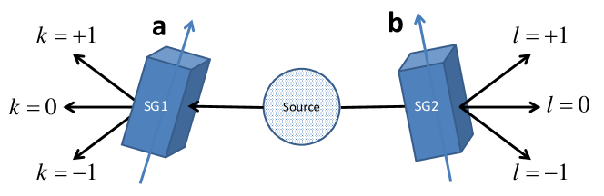
Figure 3: (Color online) Layout of the EPRB thought experiment with pairs of magnetic particles. The inhomogeneous magnetic field created by Stern-Gerlach magnet SG1 (SG2) is characterized by the unit vector $\mathbf{a}$ ($\mathbf{b}$). A particle passing through SG1 (SG2) appears in one of the beams labeled by $k=+1,0,-1$ ($l=+1,0,-1$).

XII Einstein-Podolsky-Rosen-Bohm experiment

This section is not meant to contribute to the Einstein-Bohr debate Hess (2015), related to a Gedanken-experiment suggested by Einstein-Podolsky-Rosen Einstein et al. (1935) and modified by Bohm Bohm (1951). Its purpose is to demonstrate how the quantum theoretical description follows from the application of SOC, the requirement of consistency with the description of the single- and double SG experiment developed above, and space-time continuum symmetries, without resorting to one of the postulates of quantum theory. Most importantly, this section shows, by means of the simplest example of a two-particle system, how the direct-product-of-Hilbert-spaces structure, which is characteristic for many-body quantum theory, emerges from the application of SOC.

The layout and data gathering procedure of the EPRB thought experiment that we consider is illustrated by Fig. 3. The experiment produces a data set

$${\cal D}=\big{\{}(k_{n},l_{n})\;|\;k_{n},l_{n}\in{+1,0,-1}\;;\;n=1,\ldots,N\big{\}}.$$ (97)

for each pair of settings $(\mathbf{a},\mathbf{b})$. From this data set we can compute the relative frequency of an event $(k,l)$

$$f(k,l|\mathbf{a},\mathbf{b},P,N) = \frac{1}{N}\sum_{n=1}^{N}\delta_{k,k_{n}}\delta_{l,l_{n}}.$$ (98)

The notation used and the structure are the same as before, see Eq. (7). However, the meaning of $k$ and $l$ are quite different from that in Sec. III because $k$ and $l$ refer to the detection of two particles, not of one. Therefore, we cannot proceed in a sequential manner by considering only one SG magnet and add the second one later.

As in Sec. III, we only consider the simplest case where we discard all knowledge about the events that is not contained in $f(k,l|\mathbf{a},\mathbf{b},P,N)$. Here and in the remainder of this section, the symbol $P$ indicates a conditional dependence on the properties of both particles.

Adopting the same reasoning as for the SG experiment, it follows that we cannot separate the description of the EPRB data in different parts if we stick to a representation in terms of vectors. Therefore, we simply repeat the steps that led to the matrix representation in Eq. (27) and start by writing the observations and relative frequencies as $9\times 9$ diagonal matrices

$$\left(\mathbf{\widetilde{K}}_{1}\right)_{[k,l],[k,l]}=k\quad,\quad\left(\mathbf{\widetilde{K}}_{2}\right)_{[k,l],[k,l]}=l\quad\mathrm{and}\quad\left(\mathbf{\widetilde{F}}(\mathbf{a},\mathbf{b},P,N)\right)_{[k,l],[k,l]}=f(k,l|\mathbf{a},\mathbf{b},P,N)\quad,\quad(k,l)\in{\cal E}^{2},$$ (99)

where we have introduced the notation $A_{[k,l],[k^{\prime},l^{\prime}]}=A_{i(k,l),i(k^{\prime},l^{\prime})}$ for the matrix elements of $A$ and the function $i(k,l)=2-k+3(1-l)$ is only there to map $(k,l)\in{\cal E}^{2}$ onto the standard matrix indices which run from 1 to 9. The reason for introducing two different matrices $\mathbf{\widetilde{K}}_{1}$ and $\mathbf{\widetilde{K}}_{2}$ representing the observations is that in an EPRB experiment, it is obviously necessary to distinguish between detector clicks in the left (subscript 1) and right (subscript 2) wing of the experiment, see Fig. 3.

Separating the descriptions of the source and observation stations means that we search for $9\times 9$ matrices $\mathbf{F}(P,N)$, $\mathbf{K}_{1}({\mathbf{a}})$, and $\mathbf{K}_{2}({\mathbf{b}})$ such that

$$\langle k^{p}l^{q}\rangle=\mathbf{Tr\;}\widetilde{\mathbf{F}}(P,N,\mathbf{a},\mathbf{b})\widetilde{\mathbf{K}}_{1}^{p}\widetilde{\mathbf{K}}_{2}^{q}=\mathbf{Tr\;}\mathbf{F}(P,N){\mathbf{K}}_{1}^{p}(\mathbf{a}){\mathbf{K}}_{2}^{q}(\mathbf{b})\quad,\quad p,q=0,1,2.$$ (100)

Consistency of the description with the one of the (double) SG experiments dictates that if $q=0$ ($p=0$), we must have

$$\mathbf{K}_{1}(\mathbf{a})=(\mathbf{a}\cdot\mathbf{S}_{1})\otimes\leavevmode\hbox{\small 1\normalsize\kern-3.30002pt1}\quad,\quad\mathbf{K}_{2}(\mathbf{b})=\leavevmode\hbox{\small 1\normalsize\kern-3.30002pt1}\otimes(\mathbf{b}\cdot\mathbf{S}_{2}),$$ (101)

where $\otimes$ denotes the Kronecker product and 11 is the $3\times 3$ unit matrix. Similarly, the expressions for the projections are given by

$$f(k,l|\mathbf{a},\mathbf{b},P,N)=\mathbf{Tr\;}{\mathbf{M}}_{l}^{(2)}(\mathbf{b}){\mathbf{M}}_{k}^{(1)}(\mathbf{a})\mathbf{F}(P,N){\mathbf{M}}_{k}^{(1)}(\mathbf{a}){\mathbf{M}}_{l}^{(2)}(\mathbf{b})=\mathbf{Tr\;}\mathbf{F}(P,N){\mathbf{M}}_{k}^{(1)}(\mathbf{a}){\mathbf{M}}_{l}^{(2)}(\mathbf{b}),$$ (102)

where

$${\mathbf{M}}_{k}^{(1)}(\mathbf{a})={\mathbf{M}}_{k}(\mathbf{a})\otimes\leavevmode\hbox{\small 1\normalsize\kern-3.30002pt1}\quad\hbox{and}\quad{\mathbf{M}}_{l}^{(2)}(\mathbf{b})=\leavevmode\hbox{\small 1\normalsize\kern-3.30002pt1}\otimes{\mathbf{M}}_{l}(\mathbf{b}).$$ (103)

In Sec. IX, we gave a proof that the matrix $\mathbf{F}(P,N)$ describing the source of the SG experiment is positive semidefinite. Using the same reasoning, it follows that $\mathbf{F}(P,N)$ appearing in Eq. (102) is positive semidefinite as well.

With the help of the basis in Eq. (82), we can write down the most general expression of $\mathbf{F}(P,N)$ as

$$\mathbf{F}(P,N) = \sum_{i,j=0}^{8}f_{i,j}\mathbf{B}_{i}\otimes\mathbf{B}_{j},$$ (104)

where the expansion coefficients $f_{i,j}=f^{\ast}_{j,i}$ can, in principle, be determined from the data Eq. (102), obtained by making experiments with several different choices of $(\mathbf{a},\mathbf{b})$. However, in practice, the experimental procedure to determine the 80 real numbers entering Eq. (104) is quite cumbersome. In contrast, given a specific expression for $\mathbf{F}(P,N)$, it is straightforward to compute the moments $\langle k^{p}l^{q}\rangle$. For instance, if we choose

$$\mathbf{F}(P,N)=\frac{1}{3}\left(\begin{array}[]{rrrrrrrrr}\phantom{-}0&\phantom{-}0&\phantom{-}0&\phantom{-}0&\phantom{-}0&\phantom{-}0&\phantom{-}0&\phantom{-}0&\phantom{-}0\\ \phantom{-}0&\phantom{-}0&\phantom{-}0&\phantom{-}0&\phantom{-}0&\phantom{-}0&\phantom{-}0&\phantom{-}0&\phantom{-}0\\ \phantom{-}0&\phantom{-}0&\phantom{-}1&\phantom{-}0&-1&\phantom{-}0&\phantom{-}1&\phantom{-}0&\phantom{-}0\\ \phantom{-}0&\phantom{-}0&\phantom{-}0&\phantom{-}0&\phantom{-}0&\phantom{-}0&\phantom{-}0&\phantom{-}0&\phantom{-}0\\ \phantom{-}0&\phantom{-}0&-1&\phantom{-}0&\phantom{-}1&\phantom{-}0&-1&\phantom{-}0&\phantom{-}0\\ \phantom{-}0&\phantom{-}0&\phantom{-}0&\phantom{-}0&\phantom{-}0&\phantom{-}0&\phantom{-}0&\phantom{-}0&\phantom{-}0\\ \phantom{-}0&\phantom{-}0&\phantom{-}1&\phantom{-}0&-1&\phantom{-}0&\phantom{-}1&\phantom{-}0&\phantom{-}0\\ \phantom{-}0&\phantom{-}0&\phantom{-}0&\phantom{-}0&\phantom{-}0&\phantom{-}0&\phantom{-}0&\phantom{-}0&\phantom{-}0\\ \phantom{-}0&\phantom{-}0&\phantom{-}0&\phantom{-}0&\phantom{-}0&\phantom{-}0&\phantom{-}0&\phantom{-}0&\phantom{-}0\\ \end{array}\right),$$ (114)

which, in quantum theory language, represents the pure state $|\Psi\rangle=\left(|-1,1\rangle-|0,0\rangle+|+1,-1\rangle\rangle\right)/\sqrt{3}$ with total spin zero, we obtain

$$\langle k\rangle = \mathbf{Tr\;}\mathbf{F}(P,N)\;(\mathbf{a}\cdot\mathbf{S}_{1})=\langle\mathbf{a}\cdot\mathbf{S_{1}}\rangle=0,$$

$$\langle l\rangle = \mathbf{Tr\;}\mathbf{F}(P,N)\;(\mathbf{b}\cdot\mathbf{S}_{2})=\langle\mathbf{b}\cdot\mathbf{S_{2}}\rangle=0,$$

$$\langle kl\rangle = \mathbf{Tr\;}\mathbf{F}(P,N)\;(\mathbf{a}\cdot\mathbf{S}_{1})\;(\mathbf{b}\cdot\mathbf{S}_{2})=\langle\mathbf{a}\cdot\mathbf{S_{1}}\;\mathbf{b}\cdot\mathbf{S_{2}}\rangle=-\frac{2}{3}\;\mathbf{a}\cdot\mathbf{b},$$

$$\langle k^{2}l\rangle = \mathbf{Tr\;}\mathbf{F}(P,N)\;(\mathbf{a}\cdot\mathbf{S_{1}})^{2}\;(\mathbf{b}\cdot\mathbf{S_{2}})=\langle(\mathbf{a}\cdot\mathbf{S_{1}})^{2}\;(\mathbf{b}\cdot\mathbf{S_{2}})\rangle=0,$$

$$\langle kl^{2}\rangle = \mathbf{Tr\;}\mathbf{F}(P,N)\;(\mathbf{a}\cdot\mathbf{S_{1}})\;(\mathbf{b}\cdot\mathbf{S_{2}})^{2}=\langle(\mathbf{a}\cdot\mathbf{S_{1}})\;(\mathbf{b}\cdot\mathbf{S_{2}})^{2}\rangle=0,$$

$$\langle k^{2}l^{2}\rangle = \mathbf{Tr\;}\mathbf{F}(P,N)\;(\mathbf{a}\cdot\mathbf{S_{1}})^{2}\;(\mathbf{b}\cdot\mathbf{S_{2}})^{2}=\langle(\mathbf{a}\cdot\mathbf{S_{1}})^{2}\;(\mathbf{b}\cdot\mathbf{S_{2}})^{2}\rangle=\frac{1}{3}\left(1+(\mathbf{a}\cdot\mathbf{b})^{2}\right).$$ (115)

From Eq. (115) it is clear that all the moments are invariant for arbitrary rotations of the laboratory reference frame, i.e. the matrix Eq. (114) describes a source which emits particles with properties that, upon measurement, do not change if we rotate the source.

XIII Discussion

Quantum theory allows us to describe situations in which we are unable to predict each individual event but are able to represent the collection of such events by relative frequencies only. In contrast, the key of our construction of the quantum formalism is to start from the notion of individual events. Therefore, by construction, this formulation of quantum theory is free of the usual interpretational issues related to the meaning of the density matrix/wave function and other mathematical tools, such as probability theory. In our treatment, the events are the “real thing” and the wave function only serves as a mathematical vehicle to represent the observed frequencies.

Our construction of the mathematical framework that forms the basis of quantum theory starts with the consistent application of the general and natural idea of separating descriptions in parts and of a simple rewriting of the representation of the frequencies of observed events. For concreteness, we presented an explicit construction of the quantum theoretical description for the case of the SG and EPRB experiment with three possible outcomes per particle. There is nothing in our explicit treatments that prevents generalizations to an arbitrary number of outcomes per particle and an arbitrary number of particles.

Therefore, it may be useful to discuss the relation between the various steps in our explicit construction and the commonly accepted axiomatic formulation of quantum theory. The latter is well documented von Neumann (1955); Ballentine (2003); Weinberg (2003); Khrennikov (2009). For the purpose of discussing the relation with the construction given in this paper, the formulation given in Ref. Ballentine (2003) is most convenient. We list each of them together with a reference to the point in this paper where they appear.

1. To each dynamical variable R (physical concept) there corresponds a linear operator $R$ (mathematical object), and the possible values of the dynamical variable are the eigenvalues of the operator Ballentine (2003).

   Physical concepts ultimately relate to sense impressions. As a metaphor for these impressions, we use the different outcomes of a (double) SG or EPRB experiment. The elementary mathematical objects are the projection operators $\mathbf{M}_{k}(\mathbf{e}_{z})$, see Sec. VI. More complicated mathematical objects can be constructed by appropriate linear combinations of these projection operators, exactly as in quantum theory.

2. To each state there corresponds a unique state operator. The average value of a dynamical variable R, represented by the operator $R$, in the virtual ensemble of events that may result from a preparation procedure for the state, represented by the operator $\rho$, is $\langle R\rangle=\mathbf{Tr\;}\rho R/\mathbf{Tr\;}\rho$ Ballentine (2003).

   The unique state operator, denoted by the matrix $\mathbf{F}(P,N)$ appears after separating the description of the data set into a description of the particle(s) and SG magnet(s). In Sec. IX, we show that the usual properties ($\mathbf{Tr\;}\mathbf{F}(P,N)=1$ and $\mathbf{F}(P,N)$ non-negative definite) follow from the fact that the numbers of events are non-negative numbers. The expression of the average value of a dynamical variable R follows directly from the requirement that the description separates, see Sec. IV. There is no need to consider a virtual ensemble of events.

Our derivation of the von Neumann equation and Schrödinger equation, see Sec. XI.1, builds on the theorem that the trace of a matrix is zero if and only if the matrix can be written as a commutator Shoda (1936); Albert and Muckenhoupt (1957) and the condition that the eigenvalues of $\mathbf{F}(P,N,\lambda)$ are independent of $\lambda$. SOC applied to the relative frequencies of events and elementary use of matrix algebra, together with standard assumptions about the space-time continuum, are sufficient to construct the mathematical framework of quantum theory. But even with these additional assumptions, we have $\mathrm{SOC}\models\mathrm{QT}$.

XIV Conclusion

We have explored a route to construct the mathematical framework of quantum theory without relying on the accepted set of quantum physics postulates. The Stern-Gerlach and EPRB experiment, both key to the development of quantum theory, have been used to demonstrate that the basic postulates of the quantum formalism follow from describing the number of particles in the outgoing beams in terms of separate descriptions of the individual components that make up the experiment. The SOC approach readily handles any value of the number of outcomes. The Schrödinger and the von Neumann equation, two equations governing the time evolution of quantum systems, are shown to model time-dependent data, the description of which can be separated in parts.

The general message of this paper may be summarized as follows. The idea that the description of a quantum physics experiment can be decomposed in descriptions of independent parts (e.g. preparation and measurement stage) is not only an implicit assumption in standard formulations of quantum theory but is, as we show in this paper, already sufficient to expose its basic mathematical structure embodied in Eq. (27) and generalizations thereof.

However, SOC itself does not suffice to derive, for each individual experiment, the concrete, explicit descriptions that we know from quantum theory. To this end, SOC has to be supplemented with standard assumptions about the symmetries of the space-time continuum and, as in the case of the time-dependent Schrödinger equation, with other assumptions as well. In other words, SOC can be used to describe experiments performed under different but separable conditions which may or may not be describable by the quantum formalism. In any case, the SOC-based construction of the quantum formalism explains the success of quantum theory as a tool to describe the statistics of a vast amount of (quantum or non-quantum) experiments for which we have no means to predict individual events.

Finally, we believe that the approach of introducing the quantum theoretical framework pursued in this paper may contribute to its demystification because there (i) is no need to motivate the postulates P1 and P2. and (ii) it is void of the usual postulates/interpretations regarding “wave functions”, “observables”, “quantization rules”, “Born’s rule”, “probabilities”, and the like.

Appendix A A. Rotation of the SG magnet

According to Rodrigues’ formula, rotating a unit vector $\mathbf{u}$ about the axis of rotation $\bm{\alpha}$ (with $\|\bm{\alpha}\|=1$) by an angle $\phi$ yields the vector

$$\mathbf{v}=\mathbf{u}\cos\phi+(\bm{\alpha}\times\mathbf{u})\sin\phi+(\bm{\alpha}\cdot\mathbf{u})\bm{\alpha}(1-\cos\phi)=\mathbf{u}+(\bm{\alpha}\times\mathbf{u})\sin\phi+\bm{\alpha}\times(\bm{\alpha}\times\mathbf{u})(1-\cos\phi).$$ (116)

Conversely, if $\mathbf{u}$ and $\mathbf{w}$ are unit vectors, setting

$$\bm{\alpha}=\frac{\mathbf{u}\times\mathbf{w}}{\|\mathbf{u}\times\mathbf{w}\|}=\frac{1}{\sin\phi}\mathbf{u}\times\mathbf{w}\quad,\quad\cos\phi=\mathbf{u}\cdot\mathbf{w},$$ (117)

defines the rotation about the unit vector $\bm{\alpha}$ by the angle $\phi$ which changes $\mathbf{u}$ into $\mathbf{w}$.

We now ask what happens to the projection of the spin matrices $\mathbf{S}$ on the unit vector $\mathbf{u}$ if we perform the same rotation in spin-space as the one that changes $\mathbf{u}$ into $\mathbf{w}$. To answer this question, we introduce the operator

$$g(\phi)\equiv e^{-i\,\phi\bm{\alpha}\cdot\mathbf{S}}\;\mathbf{u}\cdot\mathbf{S}\;e^{+i\,\phi\bm{\alpha}\cdot\mathbf{S}},$$ (118)

and using the commutation relations of the angular momentum (spin) operators $[S^{x},S^{y}]=iS^{z}$, $[S^{z},S^{x}]=iS^{y}$, and $[S^{y},S^{z}]=iS^{z}$ we find

$$\frac{\partial g(\phi)}{\partial\phi} = e^{-i\,\phi\bm{\alpha}\cdot\mathbf{S}}\;(\bm{\alpha}\times\mathbf{u})\cdot\mathbf{S}\;e^{+i\,\phi\bm{\alpha}\cdot\mathbf{S}},$$ (119)

$$\frac{\partial^{2}g(\phi)}{\partial\phi^{2}} = e^{-i\,\phi\bm{\alpha}\cdot\mathbf{S}}\;\bm{\alpha}\times(\bm{\alpha}\times\mathbf{u})\cdot\mathbf{S}\;e^{+i\,\phi\bm{\alpha}\cdot\mathbf{S}}=e^{-i\,\phi\bm{\alpha}\cdot\mathbf{S}}\;(\bm{\alpha}\cdot\mathbf{u})\bm{\alpha}\cdot\mathbf{S}\;e^{+i\,\phi\bm{\alpha}\cdot\mathbf{S}}-e^{-i\,\phi\bm{\alpha}\cdot\mathbf{S}}\;\mathbf{u}\cdot\mathbf{S}\;e^{+i\,\phi\bm{\alpha}\cdot\mathbf{S}}$$ (120)

$$= -g(\phi)+(\bm{\alpha}\cdot\mathbf{u})e^{-i\,\phi\bm{\alpha}\cdot\mathbf{S}}\;\bm{\alpha}\cdot\mathbf{S}\;e^{+i\,\phi\bm{\alpha}\cdot\mathbf{S}}=-g(\phi)+(\bm{\alpha}\cdot\mathbf{u})\bm{\alpha}\cdot\mathbf{S}.$$

Integrating the second-order differential equation Eq. (120) yields

$$g(\phi) = g(0)\cos\phi+g^{\prime}(0)\sin\phi+(\bm{\alpha}\cdot\mathbf{u})\bm{\alpha}\cdot\mathbf{S}(1-\cos\phi)$$ (121)

$$= \mathbf{u}\cdot\mathbf{S}\cos\phi+(\bm{\alpha}\times\mathbf{u})\cdot\mathbf{S}\sin\phi+(\bm{\alpha}\cdot\mathbf{u})\bm{\alpha}\cdot\mathbf{S}(1-\cos\phi)$$

$$= \left[\mathbf{u}\cos\phi+(\bm{\alpha}\times\mathbf{u})\sin\phi+(\bm{\alpha}\cdot\mathbf{u})\bm{\alpha}(1-\cos\phi)\right]\cdot\mathbf{S}=\mathbf{w}\cdot\mathbf{S}.$$

In other words, we have shown that a rotation in 3D space that changes a unit vector $\mathbf{u}$ into a unit vector $\mathbf{w}$ corresponds to a rotation in spin-space that changes the projection of the spin on the direction $\mathbf{u}$ to the projection of the spin on the direction $\mathbf{w}$ according to

$$\mathbf{w}\cdot\mathbf{S}=e^{-i\,\phi\bm{\alpha}\cdot\mathbf{S}}\;\mathbf{u}\cdot\mathbf{S}\;e^{+i\,\phi\bm{\alpha}\cdot\mathbf{S}}.$$ (122)

Appendix B B. Projection operators and moment expansions

We give a general proof that explicit expressions for the projectors onto the eigenspaces of a non-degenerate Hermitian matrix $A$ can be obtained by expanding an arbitrary function of the eigenvalues of $A$ in terms of its moments, and then symbolically replacing the $p$th moment by the pth power of $A$.

Let $A$ be a $N\times N$ Hermitian matrix with non-degenerate eigenvalues $\lambda_{1},\ldots,\lambda_{N}$ and corresponding eigenvectors $v_{1},\ldots,v_{N}$. The matrix

$$P_{i}(A) = \prod_{j\not=i}\frac{A-\leavevmode\hbox{\small 1\normalsize\kern-3.30002pt1}\lambda_{j}}{\lambda_{i}-\lambda_{j}}=P_{i}^{\dagger}(A),$$ (123)

satisfies $P_{i}(A)v_{k}=\delta_{i,k}v_{k}$ and $P_{j}(A)P_{i}(A)v_{k}=\delta_{i,k}\delta_{j,k}v_{k}$ and is therefore a projector on the one-dimensional space defined by the eigenvector $v_{k}$. Formally expanding the product in Eq. (123), we obtain

$$P_{i}(A) = \sum_{n=1}^{N}b_{i,n}A^{n-1}.$$ (124)

From the same formal expansion of the real-valued function defined by

$$g_{i}(\lambda) = \prod_{j\not=i}\frac{\lambda-\leavevmode\hbox{\small 1\normalsize\kern-3.30002pt1}\lambda_{j}}{\lambda_{i}-\lambda_{j}}=\sum_{n=1}^{N}b_{i,n}\lambda^{n-1},$$ (125)

it follows that

$$g_{i}(\lambda_{k}) = \delta_{i,k}=\sum_{n=1}^{N}b_{i,n}\lambda_{k}^{n-1}.$$ (126)

Introducing the Vandermonde matrix $V_{k,n}=\lambda_{k}^{n-1}$, Eq. (126) reads $bV^{\mathrm{T}}=\leavevmode\hbox{\small 1\normalsize\kern-3.30002pt1}$ or, equivalently, $b=\left(V^{\mathrm{T}}\right)^{-1}$ where the assumption that the eigenvalues are non-degenerate guarantees that the inverse of $V^{\mathrm{T}}$ exists. Therefore we may write Eq. (124) as

$$P_{i}(A) = \sum_{n=1}^{N}\left(V^{\mathrm{T}}\right)^{-1}_{i,n}A^{n-1}.$$ (127)

On the other hand, the moments $m_{p}$ of the function $f(\lambda_{1}),\ldots,f(\lambda_{N})$ are defined as

$$m_{p} = \sum_{j=1}^{N}f(\lambda_{j})\lambda_{j}^{p-1}=\sum_{j=1}^{N}f(\lambda_{j})V_{j,p}$$

$$M = V^{\mathrm{T}}F,$$ (128)

where $M=(m_{1},\ldots,m_{N})^{\mathrm{T}}$ and $F=(f(\lambda_{1}),\ldots,f(\lambda_{N}))^{\mathrm{T}}$. From Eq. (128) it follows directly that

$$F = \left(V^{\mathrm{T}}\right)^{-1}M$$

$$f(\lambda_{i}) = \sum_{p=1}^{N}\left(V^{\mathrm{T}}\right)^{-1}_{i,p}m_{p-1}.$$ (129)

Replacing the symbol $m_{p-1}$ in Eq. (129) by $A^{p-1}$, the right-hand-side of Eq. (129) becomes identical to the right-hand-side of Eq. (127), which proves the statement made in the beginning of this section.

References

- Newton (1999) I. Newton, The Principia. The Mathematical Principles of Natural Philosophy (Univ. of California Press, Berkeley, CA, 1999).
- Arnold (1990) V. I Arnold, Huygens and Barrow, Newton and Hooke: Pioneers in Mathematical Analysis and Catastrophe Theory from Evolvements to Quasicrystals (Birkh user, Basel, 1990).
- Einstein and Infeld (1967) A. Einstein and L. Infeld, The Evolution of Physics (Simon and Schuster, New York, 1967).
- Weyl (1994) H. Weyl, The Continuum: A Critical Examination of the Foundation of Analysis (Dover, Toronto, 1994).
- von Neumann (1955) J. von Neumann, Mathematical Foundations of Quantum Mechanics (Princeton University Press, Princeton, 1955).
- Weinberg (2003) S. Weinberg, Lectures on Quantum Mechanics (Cambridge University Press, Cambridge, UK, 2003).
- Rauch and Werner (2015) H. Rauch and S. A. Werner, Neutron Interferometry: Lessons in Experimental Quantum Mechanics, Wave-Particle Duality, and Entanglement (Oxford, London, 2015).
- Ballentine (2003) L. E. Ballentine, Quantum Mechanics: A Modern Development (World Scientific, Singapore, 2003).
- Barlow (1989) R. Barlow, Statistics. A Guide to the Use of Statistical Methods in the Physical Sciences (Wiley, Chichester, UK, 1989).
- Grimmet and Stirzaker (2001) G. R. Grimmet and D. R. Stirzaker, Probability and Random Processes (Clarendon Press, Oxford, 2001).
- Kolmogorov (1956) A.N. Kolmogorov, Foundations of the Theory of Probability (Chelsea Publishing Co., New York, 1956).
- Bohm (1951) D. Bohm, Quantum Theory (Prentice-Hall, New York, 1951).
- Feynman et al. (1965) R. P. Feynman, R. B. Leighton, and M. Sands, The Feynman Lectures on Physics, Vol. 3 (Addison-Wesley, Reading MA, 1965).
- Ballentine (1970) L. E. Ballentine, “The Statistical Interpretation of Quantum Mechanics,” Rev. Mod. Phys. 42, 358 – 381 (1970).
- Khrennikov (2009) A. Yu. Khrennikov, Contextual Approach to Quantum Formalism (Springer, Berlin, 2009).
- Ralston (2017) J.P. Ralston, How to Understand Quantum Mechanics (Morgan and Claypool Publishers, San Rafael, CA, 2017).
- Banach and Tarski (1924) S. Banach and A. Tarski, “Sur la décomposition des ensembles de points en parties respectivement congruentes,” Fundamenta Mathematicae 6, 244 – 277 (1924).
- Allahverdyan et al. (2017) Armen E. Allahverdyan, Roger Balian, and Theo M. Nieuwenhuizen, “A sub-ensemble theory of ideal quantum measurement processes,” Annals of Physics 376, 324 – 352 (2017).
- Khrennikov (2010) A.Y. Khrennikov, Ubiquitous Quantum Structure: From Psychology to Finance (Springer, Berlin Heidelberg, 2010).
- Bohm (1952) D. Bohm, “A Suggested Interpretation of the Quantum Theory in Terms of “Hidden” Variables. I,” Phys. Rev. 85, 166 – 179 (1952).
- de la Peña and Cetto (1996) L. de la Peña and A. M. Cetto, The Quantum Dice: An Introduction to Stochastic Electrodynamics (Kluwer, Dordrecht, 1996).
- ’t Hooft (1997) G. ’t Hooft, “Quantum mechanical behaviour in a deterministic model,” Found. Phys. Lett. 10, 105 – 111 (1997).
- de la Peña and Cetto (2005) L. de la Peña and A. M. Cetto, “Contribution from stochastic electrodynamics to the understanding of quantum mechanics,” (2005), arXiv: 0501011.
- ’t Hooft (2007) G. ’t Hooft, “The mathematical basis for deterministic quantum mechanics,” in Beyond the Quantum, edited by T. M. Nieuwenhuizen, B. Mehmani, V. S̆pic̆ka, M. J. Aghdami, and A. Yu Khrennikov (World Scientific, Singapore, 2007) pp. 3 – 19.
- Landé (1974) A. Landé, “Albert Einstein and the quantum riddle,” Am. J. Phys. 42, 459 – 464 (1974).
- Frieden (1989) B. R. Frieden, “Fisher information as the basis for the Schrödinger wave equation,” Am. J. Phys. 57, 1004 – 1008 (1989).
- Vstovsky (1995) G. V. Vstovsky, “Interpretation of the extreme physical information principle in terms of shift information,” Phys. Rev. E 51, 975 – 979 (1995).
- Reginatto (1998) M. Reginatto, “Derivation of the equations of nonrelativistic quantum mechanics using the principle of minimum Fisher information,” Phys. Rev. A 58, 1775 – 1778 (1998).
- Hardy (2001) L. Hardy, “Quantum theory from five reasonable axioms,” (2001), arXiv/quant-ph/0101012.
- Luo (2002) S. Luo, “Fisher information, kinetic energy and uncertainty relations,” J. Phys. A: Math. Gen. 35, 5181 – 5187 (2002).
- Frieden (2004) B. R. Frieden, Science from Fisher Information: A unification (Cambridge University Press, Cambridge, 2004).
- Bub (2007) J. Bub, “Quantum probabilities as degrees of belief,” Studies in History and Philosophy of Science Part B: Studies in History and Philosophy of Modern Physics 38, 232 – 254 (2007).
- Caves et al. (2007) C. M. Caves, C. A. Fuchs, and R. Schack, “Subjective probability and quantum certainty,” Studies in History and Philosophy of Science Part B: Studies in History and Philosophy of Modern Physics 38, 255 – 274 (2007).
- Palge and Konrad (2008) V. Palge and T. Konrad, “A remark on Fuchs’ Bayesian interpretation of quantum mechanics,” Studies in History and Philosophy of Science Part B: Studies in History and Philosophy of Modern Physics 39, 273 – 287 (2008).
- Kapsa et al. (2010) V. Kapsa, L. Skála, and J. Chen, “From probabilities to mathematical structure of quantum mechanics,” Physica E 42, 293 – 297 (2010).
- Chiribella et al. (2011) G. Chiribella, G. M. D’Ariano, and P. Perinotti, “Informational derivation of quantum theory,” Phys. Rev. A 84, 012311 (2011).
- Masanes and Müller (2011) L. Masanes and M. P. Müller, “A derivation of quantum theory from physical requirements,” New J. Phys. 13, 063001 (2011).
- Brukner (2011) Č. Brukner, “Questioning the rules of the game,” Physics 4, 55 (2011).
- Skála et al. (2011) L. Skála, J. Ĉízêk, and V. Kapsa, “Quantum Mechanics as applied mathematical statistics,” Ann. Phys. 326, 1174 – 1188 (2011).
- Kapsa and Skála (2011) V. Kapsa and L. Skála, “Quantum Mechanics, Probabilities and Mathematical Statistics,” J. Comput. Theor. Nanosci. 8, 998 – 1005 (2011).
- Oreshkov et al. (2012) O. Oreshkov, F. Costa, and Č. Brukner, “Quantum correlations with no causal order,” Nat. Comm. 3, 1 – 8 (2012).
- Santamato and De Martini (2012) E. Santamato and F. De Martini, “Solving the Quantum Nonlocality Enigma by Weyl’s Conformal Geometrodynamics,” (2012), arXiv/quant-ph/1203.0033.
- Klein (2010) U. Klein, “The statistical origins of quantum mechanics,” Physics Research International 2010, 808424 (2010).
- Flego et al. (2012) S. P. Flego, A. Plastino, and A. R. Plastino, “Fisher information and quantum mechanics,” Int. Res. J. Pure & Appl. Chem. 2, 25 – 54 (2012).
- Kapustin (2013) A. Kapustin, “Is quantum mechanics exact?” J. Math. Phys 54, 062017 (2013).
- Fuchs and Schack (2013) C. A. Fuchs and R. Schack, “Quantum-Bayesian Coherence,” Rev. Mod. Phys. 85, 1693 – 1715 (2013).
- Holik et al. (2014) F. Holik, M. Sáenz, and A. Plastino, “A discussion on the origin of quantum probabilities,” Ann. Phys. 340, 293 – 310 (2014).
- Ralston (2013) J. P. Ralston, “Emergent mechanics, quantum and un-quantum,” Proc. SPIE 8832, 88320W1–25 (2013).
- Cox (1946) R. T. Cox, “Probability, Frequency and Reasonable Expectation,” Am. J. Phys. 14, 1 – 13 (1946).
- Cox (1961) R. T. Cox, The Algebra of Probable Inference (Johns Hopkins University Press, Baltimore, 1961).
- Tribus (1999) M. Tribus, Rational Descriptions, Decisions and Designs (Expira Press, Stockholm, 1999).
- Smith and Erickson (1989) C. R. Smith and G. Erickson, “From Rationality and consistency to Bayesian probability,” in Maximum Entropy and Bayesian Methods, edited by J. Skilling (Kluwer Academic Publishers, Dordrecht, 1989) pp. 29 – 44.
- Jaynes (2003) E. T. Jaynes, Probability Theory: The Logic of Science (Cambridge University Press, Cambridge, 2003).
- De Raedt et al. (2014) H. De Raedt, M. I. Katsnelson, and K. Michielsen, “Quantum theory as the most robust description of reproducible experiments,” Ann. Phys. 347, 45 – 73 (2014).
- De Raedt et al. (2016) H. De Raedt, M. I. Katsnelson, and K. Michielsen, “Quantum theory as plausible reasoning applied to data obtained by robust experiments,” Phil. Trans. R. Soc. A 374, 20150233 (2016).
- De Raedt et al. (2015a) H. De Raedt, M. I. Katsnelson, H. C. Donker, and K. Michielsen, “Quantum theory as a description of robust experiments: derivation of the Pauli equation,” Ann. Phys. 359, 166 – 186 (2015a).
- Donker et al. (2016) H.C. Donker, M.I. Katsnelson, H. De Raedt, and K. Michielsen, “Logical inference approach to relativistic quantum mechanics: Derivation of the Klein-Gordon equation,” Ann. Phys 372, 74 – 82 (2016).
- De Raedt et al. (2013) H. De Raedt, M. I. Katsnelson, and K. Michielsen, “Quantum theory as the most robust description of reproducible experiments: application to a rigid linear rotator,” Proc. SPIE 8832, 883212–1–11 (2013).
- De Raedt et al. (2015b) H. De Raedt, M. I. Katsnelson, H. C. Donker, and K. Michielsen, “Quantum theory as a description of robust experiments: Application to Stern-Gerlach and Einstein-Podolsky-Rosen-Bohm experiments,” Proc. SPIE 9570, 95700–1–14 (2015b).
- De Raedt et al. (2018) H. De Raedt, M. I. Katsnelson, and K. Michielsen, “Logical inference derivation of the quantum theoretical description of Stern-Gerlach and Einstein-Podolsky-Rosen-Bohm experiments,” Ann. Phys. 396, 96 – 118 (2018).
- Heisenberg (1925) W. Heisenberg, “Über quantentheoretische Umdeutung kinematischer und mechanischer Beziehungen,” Z. Phys. 33, 879 – 893 (1925).
- Gerlach and Stern (1922) W. Gerlach and O. Stern, “Der experimentelle Nachweis der Richtungsquantelung im Magnetfeld,” Z. Phys. 9, 349 – 352 (1922).
- Gerlach and Stern (1924) W. Gerlach and O. Stern, “Über die Richtungsquantelung im Magnetfeld,” Ann. Phys. 74, 673 – 699 (1924).
- Sherwood et al. (1954) J. E. Sherwood, T. K. Stephenson, and S. Bernstein, “Stern-Gerlach experiment on polarized neutrons,” Phys. Rev. 96, 1546 – 1548 (1954).
- Hamelin et al. (1975) B. Hamelin, N. Xiromeritis, and P. Liaud, “Calcul, montage et experimentation d’un nouveau type d’aimant de “Stern et Gerlach comme polariseur ou analyseur de polarisation des neutrons,” Nucl. Instrum. Methods 125, 79 – 84 (1975).
- Batelaan et al. (1997) H. Batelaan, T. J. Gay, and J. J. Schwendiman, “Stern-Gerlach effect for electron beams,” Phys. Rev. Lett. 79, 4517 – 4521 (1997).
- Diaz-Bachs et al. (2018) A. Diaz-Bachs, M. I. Katsnelson, and A. Kirilyuk, “Kramers degeneracy and relaxation in vanadium, niobium and tantalum clusters,” New J. Phys. 20, 043042 (2018).
- Born (1926) M. Born, “Zur Quantenmechanik der Stoßvorgänge,” Z. Phys. 37, 863 – 867 (1926).
- Shoda (1936) K. Shoda, “Einige Sätze über Matrizen,” Jap. J. Math. 13, 361–365 (1936).
- Albert and Muckenhoupt (1957) A. A. Albert and B. Muckenhoupt, “On matrices of trace zeros,” Michigan Math. J. , 1–3 (1957).
- Schrödinger (1926a) E. Schrödinger, “Über das Verhältnis der Heisenberg-Born-Jordanischen Quantenmechanik zu der meinen,” Ann. Phys. (Berlin) 79, 734 – 756 (1926a).
- Breuer and Petruccione (2002) H.-P. Breuer and F. Petruccione, The Theory of Open Quantum Systems (Oxford University Press, Oxford, 2002).
- Abragam and Bleeney (1970) A. Abragam and B. Bleeney, Electron Paramagnetic Resonance of Transition Ions (Clarendon Press, Oxford, 1970).
- Schrödinger (1926b) E. Schrödinger, “Quantisierung als Eigenwertproblem (Erste Mitteilung),” Ann. Phys. (Berlin) 384, 361 – 376 (1926b).
- Jordan (1969) T.F. Jordan, Linear Operators for Quantum Mechanics (Wiley, New York, 1969).
- Hess (2015) K. Hess, Einstein Was Right! (Pan Stanford Publishing, Singapore, 2015).
- Einstein et al. (1935) A. Einstein, A. Podolsky, and N. Rosen, “Can quantum-mechanical description of physical reality be considered complete?” Phys. Rev. 47, 777 – 780 (1935).