Learning over Multitask Graphs –
Part I: Stability Analysis

Abstract

This paper formulates a multitask optimization problem where agents in the network have individual objectives to meet, or individual parameter vectors to estimate, subject to a smoothness condition over the graph. The smoothness condition softens the transition in the tasks among adjacent nodes and allows incorporating information about the graph structure into the solution of the inference problem. A diffusion strategy is devised that responds to streaming data and employs stochastic approximations in place of actual gradient vectors, which are generally unavailable. The approach relies on minimizing a global cost consisting of the aggregate sum of individual costs regularized by a term that promotes smoothness. We show in this Part I of the work, under conditions on the step-size parameter, that the adaptive strategy induces a contraction mapping and leads to small estimation errors on the order of the small step-size. The results in the accompanying Part II will reveal explicitly the influence of the network topology and the regularization strength on the network performance and will provide insights into the design of effective multitask strategies for distributed inference over networks.

I Introduction

Distributed inference allows a collection of interconnected agents to perform parameter estimation tasks from streaming data by relying solely on local computations and interactions with immediate neighbors. Most prior literature focuses on single-task problems, where agents with separable objective functions need to agree on a common parameter vector corresponding to the minimizer of an aggregate sum of individual costs [2, 3, 4, 5, 6, 7, 8, 9, 10, 11]. Many network applications require more complex models and flexible algorithms than single-task implementations since their agents may need to estimate and track multiple objectives simultaneously [12, 13, 14, 15, 16, 17, 18, 19, 20, 21, 22]. Networks of this kind are referred to as multitask networks. Although agents may generally have distinct though related tasks to perform, they may still be able to capitalize on inductive transfer between them to improve their performance.

Based on the type of prior information that may be available about how the tasks are related to each other, multitask learning algorithms can be derived by translating the prior information into constraints on the parameter vectors to be inferred [12, 13, 14, 15, 16, 17, 18, 19, 20, 21, 22]. For example, in [18, 19, 20], distributed strategies are developed under the assumption that the parameter vectors across the agents overlap partially. A more general scenario is considered in [21] where it is assumed that the tasks across the agents are locally coupled through linear equality constraints. In [22], the parameter space is decomposed into two orthogonal subspaces, with one of the subspaces being common to all agents. There is yet another useful way to model relationships among tasks, namely, to formulate optimization problems with appropriate regularization terms encoding these relationships [13, 14, 15, 16, 17]. For example, the strategy developed in [13] adds squared $\ell_{2}$-norm co-regularizers to the mean-square-error criterion to promote task similarities, while the strategy in [14] adds $\ell_{1}$-norm co-regularizers to promote piece-wise constant transitions.

In this paper, and the accompanying Part II [23], we consider multitask inference problems where each agent in the network seeks to minimize an individual cost expressed as the expectation of some loss function. The minimizers of the individual costs are assumed to vary smoothly on the topology captured by the graph Laplacian matrix. The smoothness property softens the transition in the tasks among adjacent nodes and allows incorporating information about the graph structure into the solution of the inference problem. In order to exploit the smoothness prior, we formulate the inference problem as the minimization of the aggregate sum of individual costs regularized by a term promoting smoothness, known as the graph-Laplacian regularizer [24, 25]. A diffusion strategy is devised that responds to streaming data and employs stochastic approximations in place of actual gradient vectors, which are generally unavailable. We show in this Part I of the work, under conditions on the step-size learning parameter $\mu$, that the adaptive strategy induces a contraction mapping and that despite gradient noise, it is able to converge in the mean-square-error sense within $O(\mu)$ from the solution of the regularized problem, for sufficiently small $\mu$. The analysis in the current part also reveals how the regularization strength $\eta$ can steer the convergence point of the network toward many modes starting from the non-cooperative mode where each agent converges to the minimizer of its individual cost and ending with the single-task mode where all agents converge to a common parameter vector corresponding to the minimizer of the aggregate sum of individual costs. We shall also derive in Part II [23] a closed-form expression for the steady-state network mean-square-error relative to the minimizer of the regularized cost. This closed form expression will reveal explicitly the influence of the regularization strength, network topology, gradient noise, and data characteristics, on the network performance. Additionally, a closed-form expression for the steady-state network mean-square-error relative to the minimizers of the individual costs will be also derived in Part II [23]. This expression will provide insights into the design of effective multitask strategies for distributed inference over networks.

There have been many works in the literature studying distributed multitask adaptive strategies and their convergence behavior. Nevertheless, with few exceptions [20], most of these works focus on mean-square-error costs. This paper, and the accompanying Part II [23], generalize distributed multitask inference over networks and applies it to a wide class of individual costs. Furthermore, previous works in this domain tend to show the benefit of multitask learning empirically by simulations. Following some careful and demanding analysis, we establish in Part II [23], which builds on the results of this Part I, a useful expression for the network steady-state performance. This expression provides insights into the learning behavior of multitask networks and clarifies how multitask distributed learning may improve the network performance.

Notation. All vectors are column vectors. Random quantities are denoted in boldface. Matrices are denoted in capital letters while vectors and scalars are denoted in lower-case letters. The operator $\preceq$ denotes an element-wise inequality; i.e., $a\preceq b$ implies that each entry of the vector $a$ is less than or equal to the corresponding entry of $b$. The symbol $\text{diag}\{\cdot\}$ forms a matrix from block arguments by placing each block immediately below and to the right of its predecessor. The operator $\text{col}\{\cdot\}$ stacks the column vector entries on top of each other. The symbol $\otimes$ denotes the Kronecker product.

II Distributed inference under smoothness priors

II-A Problem formulation and adaptive strategy

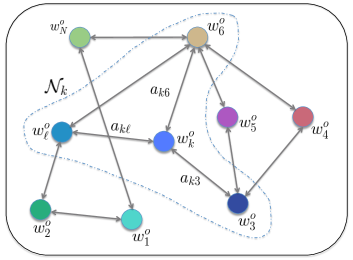
Figure 1: Agents linked by an edge can share information. The weight $a_{k\ell}$ over an edge reflects the strength of the relation between $w^{o}_{k}$ at node $k$ and $w^{o}_{\ell}$ at node $\ell$.

We refer to Fig. 1 and consider a connected network (or graph) $\mathcal{G}=\{\mathcal{N},\mathcal{E},A\}$, where $\mathcal{N}$ is a set of $N$ agents (nodes), $\mathcal{E}$ is a set of edges connecting agents with particular relations, and $A$ is a symmetric, weighted adjacency matrix. If there is an edge connecting agents $k$ and $\ell$, then $[A]_{k\ell}=a_{k\ell}>0$ reflects the strength of the relation between $k$ and $\ell$; otherwise, $[A]_{k\ell}=0$. We introduce the graph Laplacian $L$, which is a differential operator defined as $L=D-A$, where the degree matrix $D$ is a diagonal matrix with $k$-th entry $[D]_{kk}=\sum_{\ell=1}^{N}a_{k\ell}$. Since $L$ is symmetric positive semi-definite, it possesses a complete set of orthonormal eigenvectors. We denote them by $\{v_{1},\ldots,v_{N}\}$. For convenience, we order the set of real, non-negative eigenvalues of $L$ as $0=\lambda_{1}<\lambda_{2}\leq\ldots\leq\lambda_{N}=\lambda_{\max}(L)$, where, since the network is connected, there is only one zero eigenvalue with corresponding eigenvector $v_{1}=\frac{1}{\sqrt{N}}\mathds{1}_{N}$ [26]. Thus, the Laplacian can be decomposed as:

$$L=V\Lambda V^{\top},$$ (1)

where $\Lambda=\text{diag}\{\lambda_{1},\ldots,\lambda_{N}\}$ and $V=[v_{1},\ldots,v_{N}]$.

Let $w_{k}\in\mathbb{R}^{M}$ denote some parameter vector at agent $k$ and let ${\scriptstyle\mathcal{W}}=\text{col}\{w_{1},\ldots,w_{N}\}$ denote the collection of parameter vectors from across the network. We associate with each agent $k$ a risk function $J_{k}(w_{k}):\mathbb{R}^{M}\rightarrow\mathbb{R}$ assumed to be strongly convex. In most learning and adaptation problems, the risk function is expressed as the expectation of a loss function $Q_{k}(\cdot)$ and is written as $J_{k}(w_{k})=\mathbb{E}\,Q_{k}(w_{k};\boldsymbol{x}_{k})$, where $\boldsymbol{x}_{k}$ denotes the random data. The expectation is computed over the distribution of this data. We denote the unique minimizer of $J_{k}(w_{k})$ by $w^{o}_{k}$. We introduce a common assumption on the risks $\{J_{k}(w_{k})\}$. This condition is applicable to many situations of interest (see, e.g., [7, 10]).

Assumption 1.

(Strong convexity) It is assumed that the individual costs $J_{k}(w_{k})$ are each twice differentiable and strongly convex such that the Hessian matrix function $H_{k}(w_{k})=\nabla^{2}_{w_{k}}J_{k}(w_{k})$ is uniformly bounded from below and above, say, as:

$$0<\lambda_{k,\min}I_{M}\leq H_{k}(w_{k})\leq\lambda_{k,\max}I_{M},$$ (2)

where $\lambda_{k,\min}>0$ for $k=1,\ldots,N$. ∎

In many situations, there is prior information available about ${\scriptstyle\mathcal{W}}^{o}=\text{col}\{w_{1}^{o},\ldots,w_{N}^{o}\}$. In the current work, the prior belief we want to enforce is that the target signal ${\scriptstyle\mathcal{W}}^{o}$ is smooth with respect to the underlying weighted graph. References [13, 14, 15] provide variations for such problems for the special case of mean-square-error costs. Here we treat general convex costs. Let $\mathcal{L}=L\otimes I_{M}$. The smoothness of ${\scriptstyle\mathcal{W}}$ can be measured in terms of a quadratic form of the graph Laplacian [24, 25, 27]:

$$S({\scriptstyle\mathcal{W}})={\scriptstyle\mathcal{W}}^{\top}\mathcal{L}{\scriptstyle\mathcal{W}}=\frac{1}{2}\sum_{k=1}^{N}\sum_{\ell\in\mathcal{N}_{k}}a_{k\ell}\|w_{k}-w_{\ell}\|^{2},$$ (3)

where $\mathcal{N}_{k}$ is the set of neighbors of $k$, i.e., the set of nodes connected to agent $k$ by an edge. Figure 1 provides an illustration. The smaller $S({\scriptstyle\mathcal{W}})$ is, the smoother the signal ${\scriptstyle\mathcal{W}}$ on the graph is. Intuitively, given that the weights are non-negative, $S({\scriptstyle\mathcal{W}})$ shows that ${\scriptstyle\mathcal{W}}$ is considered to be smooth if nodes with a large $a_{k\ell}$ on the edge connecting them have similar weight values $\{w_{k},w_{\ell}\}$. Our objective is to devise and study a strategy that solves the following regularized problem:

$${\scriptstyle\mathcal{W}}^{o}_{\eta}=\arg\min_{{\scriptstyle\mathcal{W}}}J^{\text{glob}}({\scriptstyle\mathcal{W}})=\sum_{k=1}^{N}J_{k}(w_{k})+\frac{\eta}{2}\,{\scriptstyle\mathcal{W}}^{\top}\mathcal{L}{\scriptstyle\mathcal{W}},$$ (4)

in a distributed manner where each agent is interested in estimating the $k$-th sub-vector of ${\scriptstyle\mathcal{W}}^{o}_{\eta}=\text{col}\{w_{1,\eta}^{o},\ldots,w_{N,\eta}^{o}\}$. The tuning parameter $\eta\geq 0$ controls the trade-off between the two components of the objective function. Reference [1] provides a theoretical motivation for the optimization framework where it is shown that, under a Gaussian Markov random field assumption, solving problem (4) is equivalent to finding a maximum a posteriori (MAP) estimate for $\boldsymbol{{\scriptstyle\mathcal{W}}}$. We are particularly interested in solving the problem in the stochastic setting when the distribution of the data $\boldsymbol{x}_{k}$ in $J_{k}(w_{k})=\mathbb{E}\,Q_{k}(w_{k};\boldsymbol{x}_{k})$ is generally unknown. This means that the risks $J_{k}(w_{k})$ and their gradients $\nabla_{w_{k}}J_{k}(w_{k})$ are unknown. As such, approximate gradient vectors need to be employed. A common construction in stochastic approximation theory is to employ the following approximation at iteration $i$:

$$\widehat{\nabla_{w_{k}}J_{k}}(w_{k})=\nabla_{w_{k}}Q_{k}(w_{k};\boldsymbol{x}_{k,i}),$$ (5)

where $\boldsymbol{x}_{k,i}$ represents the data observed at iteration $i$. The difference between the true gradient and its approximation is called the gradient noise $\boldsymbol{s}_{k,i}(\cdot)$:

$$\boldsymbol{s}_{k,i}(w)\triangleq\nabla_{w_{k}}J_{k}(w)-\widehat{\nabla_{w_{k}}J_{k}}(w).$$ (6)

Each agent can employ a stochastic gradient descent update to estimate $w^{o}_{k,\eta}$:

$$\boldsymbol{w}_{k,i}=\boldsymbol{w}_{k,i-1}-\mu\widehat{\nabla_{w_{k}}J_{k}}(\boldsymbol{w}_{k,i-1})-\mu\eta\sum_{\ell\in\mathcal{N}_{k}}a_{k\ell}(\boldsymbol{w}_{k,i-1}-\boldsymbol{w}_{\ell,i-1}),$$ (7)

where $\mu>0$ is a small step-size parameter. In this implementation, each agent $k$ collects from its neighbors the estimates $\boldsymbol{w}_{\ell,i-1}$, and performs a stochastic-gradient descent update on:

$$\bar{J}_{k,i-1}(w_{k})\triangleq J_{k}(w_{k})+\frac{\eta}{2}\sum_{\ell\in\mathcal{N}_{k}}a_{k\ell}\|w_{k}-\boldsymbol{w}_{\ell,i-1}\|^{2}.$$ (8)

By introducing an auxiliary variable $\boldsymbol{\psi}_{k,i}$, strategy (7) can be implemented in an incremental manner:

$$\left\{\begin{array}[]{lr}\boldsymbol{\psi}_{k,i}=\boldsymbol{w}_{k,i-1}-\mu\widehat{\nabla_{w_{k}}J_{k}}(\boldsymbol{w}_{k,i-1})\\ \boldsymbol{w}_{k,i}=\boldsymbol{\psi}_{k,i}-\mu\eta\displaystyle\sum_{\ell\in\mathcal{N}_{k}}a_{k\ell}(\boldsymbol{\psi}_{k,i}-\boldsymbol{\psi}_{\ell,i}),\end{array}\right.$$ (9)

where we replaced $(\boldsymbol{w}_{k,i-1}-\boldsymbol{w}_{\ell,i-1})$ in the second step by the difference $(\boldsymbol{\psi}_{k,i}-\boldsymbol{\psi}_{\ell,i})$ since we expect $\boldsymbol{\psi}_{k,i}$ to be an improved estimate compared to $\boldsymbol{w}_{k,i-1}$. Note that if we introduce the coefficients:

$$c_{k\ell}=\left\{\begin{array}[]{ll}1-\mu\eta\displaystyle\sum_{\ell\in\mathcal{N}_{k}}a_{k\ell},&k=\ell\\ \mu\eta a_{k\ell},&\ell\in\mathcal{N}_{k}\setminus\{k\}\\ 0,&\ell\notin\mathcal{N}_{k}\end{array}\right.$$ (10)

then recursion (9) can be written in the diffusion form[6, 7, 8, 9, 10]:

$$\left\{\begin{array}[]{lr}\boldsymbol{\psi}_{k,i}=\boldsymbol{w}_{k,i-1}-\mu\widehat{\nabla_{w_{k}}J_{k}}(\boldsymbol{w}_{k,i-1})\\ \boldsymbol{w}_{k,i}=\displaystyle\sum_{\ell\in\mathcal{N}_{k}}c_{k\ell}\boldsymbol{\psi}_{\ell,i},\end{array}\right.$$ (11)

where the second step is a combination step. If we collect the scalars $\{c_{k\ell}\}$ into the matrix $C=[c_{k\ell}]$, then the entries of $C$ are non-negative for small enough $\mu$ and its columns and rows add up to one, i.e., $C$ is a doubly-stochastic matrix. We shall continue with form (9) because the second step in (9) makes the dependence on $\eta$ explicit. We will show later that by varying the value of $\eta$ we can make the algorithm behave in different ways from fully non-cooperative to fully single-task with many other modes in between.

II-B Summary of main results

Before delving into the study of the learning capabilities of (9) and its performance limits, we summarize in this section, for the benefit of the reader, the main conclusions of this Part I, and its accompanying Part II [23]. One key insight that will follow from the detailed analysis in this Part I is that the smoothing parameter $\eta$ can be regarded as an effective tuning parameter that controls the nature of the learning process. The value of $\eta$ can vary from $\eta=0$ to $\eta\rightarrow\infty$. We will show that at one end, when $\eta=0$, the learning algorithm reduces to a non-cooperative mode of operation where each agent acts individually and estimates its own local model, $w^{o}_{k}$. On the other hand, when $\eta\rightarrow\infty$, the learning algorithm moves to a single-mode of operation where all agents cooperate to estimate a single parameter (namely, the Pareto solution of the aggregate cost function). For any values of $\eta$ in the range $0<\eta<\infty$, the network behaves in a multitask mode where agents seek their individual models while at the same time ensuring that these models satisfy certain smoothness and closeness conditions dictated by the value of $\eta$. We are not only interested in a qualitative description of the network behavior. Instead, we would like to characterize these models in a quantitative manner by deriving expressions that allow us to predict performance as a function of $\eta$ and, therefore, fine tune the network to operate in different scenarios.

To begin with, recall that the objective of the multitask strategy (9) is to exploit similarities among neighboring agents in an attempt to improve the overall network performance in approaching the collection of individual minimizer ${{\scriptstyle\mathcal{W}}}^{o}$ by means of local communications. In light of the fact that algorithm (9) has been derived as an (incremental) gradient descent recursion for the regularized cost (4), whose minimizer ${\scriptstyle\mathcal{W}}_{\eta}^{o}$ is in general different from ${\scriptstyle\mathcal{W}}^{o}$, the limiting point of algorithm (9) will therefore be generally different from ${\scriptstyle\mathcal{W}}^{o}$, the actual objective of the multitask learning problem. This mismatch is the “cost” of enforcing smoothness. The analysis in the paper will reveal that the mismatch is a function of the similarity between the individual minimizers $\{w_{k}^{o}\}$, of second-order properties of the individual costs, of the network topology captured by $L$, and of the regularization strength $\eta$. In particular, future expression (31) will allow us to understand the interplay between these quantities which is important for the design of effective multitask strategies. The key conclusion will be that, while the bias (difference between ${\scriptstyle\mathcal{W}}_{\eta}^{o}$ and ${\scriptstyle\mathcal{W}}^{o}$) will in general increase as the regularization strength $\eta$ increases, the size of this increase is determined by the smoothness of ${\scriptstyle\mathcal{W}}^{o}$ which is in turn function of the network topology captured by $L$. The more similar the tasks at neighboring agents are, the smaller the bias will be. This result, while intuitive, is reassuring, as it implies that as long as ${\scriptstyle\mathcal{W}}^{o}$ is sufficiently smooth, the bias induced by regularization will remain small, even for moderate regularization strengths $\eta$.

The analysis also quantifies the benefit of cooperation, namely, the objective of improving the mean-square deviation around the limiting point of the algorithm. This analysis is challenging due to coupling among agents, and the multi-task nature of the learning process (where agents have individual targets but need to meet certain smoothness and closeness conditions with their neighbors). Section III in this Part I and Sections III and IV in Part II [23], and the supporting appendices, are devoted to carrying out this analysis in depth leading, for example to Theorem 1 in Part II [23]. This theorem gives expressions for the mean-square-deviation (MSD) relative to ${\scriptstyle\mathcal{W}}_{\eta}^{o}$. The expressions reveal the effect of the step-size parameter $\mu$, regularization strength $\eta$, network topology, and data characteristics (captured by the smoothness profile, second-order properties of the costs, and second-order moments of the gradient noise) on the size of the steady-state mean-square-error performance. The results established in Theorem 1 and expression (82) in Part II [23] provide tools for characterizing the performance of multitask strategies in some great detail.

To illustrate the power of these results, consider a connected network where each agent is subjected to streaming data. The goal at each agent is to estimate a local parameter vector $w^{o}_{k}$ from the observed data by minimizing a cost of the form $J_{k}(w_{k})=\mathbb{E}\,Q_{k}(w_{k};\boldsymbol{x}_{k})$, where $\boldsymbol{x}_{k}$ denotes the random data. Consider network applications where the minimizers at neighboring agents tend to be similar [13, 25]. Although each agent is interested in estimating its own task $w^{o}_{k}$, cooperating neighboring agents can still benefit from their interactions because of this closeness. Given the graph Laplacian and data characteristics, one problem of interest would be to determine the optimal cooperation rule, i.e., the value of $\eta$ that minimizes the network mean-square-error performance. Future expression (82) in Part II [23] can be used to solve this problem since it allows us to predict the network MSD relative to ${\scriptstyle\mathcal{W}}^{o}$. By using expression (82) in Part II [23], for example, we will be able to construct curves of the form shown in Fig. 2, which illustrate how performance is dependent on the smoothness parameter $\eta$ and how the nature of the limiting solution varies as a function of this parameter. As it can be seen from this figure, $\eta=4$ gives the best network steady-state mean-square performance. Note that $\eta=0$ corresponds to the non-cooperative scenario and that a large $\eta$ induces a large bias in the estimation. In the sequel we will show that as $\eta$ varies from $\eta=0$ to $\eta\rightarrow\infty$, the network behavior moves from the non-cooperative mode of operation (where agents act independently) to the single-task mode of operation (where all agents focus on estimating a single parameter). For values of $\eta$ in between, the network can operate in any of a multitude of multitask modes (where agents estimate their own local parameters under smoothness conditions to allow for some similarity between adjacent nodes). These limits are indicated in Fig. 2.

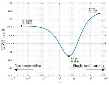
Figure 2: Network steady-state MSD relative to a smooth signal ${\scriptstyle\mathcal{W}}^{o}$ as a function of the regularization strength $\eta\in[0,350]$ at $\mu=0.005$.

Finally, we would like to mention that one of the main tools used in the analysis in this work, and its accompanying Part II [23], is the linear transformation relative to the eigenspace of the graph Laplacian $L$ from [6], which is also known as the graph Fourier transform [25, 28, 29]. Under some conditions on the data and costs profile, we show in Section VI-A in Part II [23] how the diffusion type algorithm (9) exhibits a low-pass graph filter behavior. Such filters are commonly used to reduce the network noise profile when the signal to be estimated is smooth with respect to the underlying topology [25, 30, 31, 32]. Interestingly, the theoretical results established in this Part I, and its accompanying Part II [23], reveal the reasons for performance improvements under localized cooperation.

II-C Network limit point and regularization strength

Before examining the behavior and performance of strategy (9) with respect to the limiting point ${\scriptstyle\mathcal{W}}^{o}_{\eta}$ in (4), we discuss the influence of $\eta$ on ${\scriptstyle\mathcal{W}}^{o}_{\eta}$. When $\eta=0$, we have from (4) that ${\scriptstyle\mathcal{W}}^{o}_{\eta}={\scriptstyle\mathcal{W}}^{o}$ and strategy (9) reduces to the single-agent mode of operation or the non-cooperative solution where each agent minimizes $J_{k}(w_{k})$ locally without cooperation. When $\eta\rightarrow\infty$, we have from (4) that ${\scriptstyle\mathcal{W}}^{o}_{\eta}=\mathds{1}_{N}\otimes w^{\star}$ where

$$w^{\star}\triangleq\arg\min_{w}\sum_{k=1}^{N}J_{k}(w),$$ (12)

and we are in the single-task mode of operation where all agents seek to estimate a common parameter vector $w^{\star}$ corresponding to the minimizer of the aggregate sum of individual costs [7, 6, 8, 9, 10]. In order to study more closely the influence of (finite) $\eta>0$ on the network output ${\scriptstyle\mathcal{W}}^{o}_{\eta}$, we examine the influence of $\eta$ on the transformed vector:

$$\overline{{\scriptstyle\mathcal{W}}}^{o}_{\eta}\triangleq(V^{\top}\otimes I_{M}){\scriptstyle\mathcal{W}}^{o}_{\eta}=\text{col}\left\{{\overline{w}^{o}_{m,\eta}}\right\}_{m=1}^{N},$$ (13)

with the $m$-th sub-vector $\overline{w}^{o}_{m,\eta}$ denoting the spectral content of ${\scriptstyle\mathcal{W}}^{o}_{\eta}$ at the $m$-th eigenvalue $\lambda_{m}$ of the Laplacian:

$${\overline{w}^{o}_{m,\eta}}=(v_{m}^{\top}\otimes I_{M})\overline{{\scriptstyle\mathcal{W}}}^{o}_{\eta}.$$ (14)

From (1), the quadratic regularization term $S({\scriptstyle\mathcal{W}})$ in (3) can be written as:

$$S({\scriptstyle\mathcal{W}})={\scriptstyle\mathcal{W}}^{\top}\mathcal{L}{\scriptstyle\mathcal{W}}=\sum_{m=1}^{N}\lambda_{m}\|{\overline{w}_{m}}\|^{2}=\sum_{m=2}^{N}\lambda_{m}\|{\overline{w}_{m}}\|^{2},$$ (15)

where ${\overline{w}_{m}}=(v_{m}^{\top}\otimes I_{M}){\scriptstyle\mathcal{W}}$ and where we used the fact that $\lambda_{1}=0$. Intuitively, given that $\lambda_{m}>0$ for $m=2,\ldots,N$, the above expression shows that ${\scriptstyle\mathcal{W}}$ is considered to be smooth if $\|{\overline{w}_{m}}\|^{2}$ corresponding to large $\lambda_{m}$ is small. As a result, for a fixed $\lambda_{m}>0$, and as the regularization strength $\eta>0$ in (4) increases, one would expect $\|{\overline{w}^{o}_{m,\eta}}\|^{2}$ to decrease. Similarly, for a fixed $\eta\geq 0$, and as $\lambda_{m}>0$ increases, one would expect $\|{\overline{w}^{o}_{m,\eta}}\|^{2}$ to decrease as well. However, as we will see in the sequel, this behavior does not always hold. We show in Section VI-A in Part II [23] that this is valid when the Hessian matrix function $H_{k}(w_{k})\triangleq\nabla^{2}_{w_{k}}J_{k}(w_{k})$ is independent of $w_{k}$, i.e., the cost $J_{k}(w_{k})$ is quadratic in $w_{k}$ and is uniform across the network. For more general scenarios, this is not necessarily the case. What is useful to note, however, is that as $\eta$ moves from $0$ towards $\infty$, a variety of solution points ${\scriptstyle\mathcal{W}}^{o}_{\eta}$ can occur ranging from the non-cooperative to the single-task solution at both extremes.

From the optimality condition of (4), we have:

$$\text{col}\left\{\nabla_{w_{k}}J_{k}(w_{k,\eta}^{o})\right\}_{k=1}^{N}=-\eta\mathcal{L}{\scriptstyle\mathcal{W}}^{o}_{\eta},$$ (16)

Using the mean value theorem [33, pp. 24], we can write:

$$\nabla_{w_{k}}J_{k}(w_{k,\eta}^{o})-{\underbrace{\nabla_{w_{k}}J_{k}(w_{k}^{o})}_{=0}}=H^{o}_{k,\eta}(w_{k,\eta}^{o}-w_{k}^{o}),$$ (17)

where

$$H^{o}_{k,\eta}\triangleq\int_{0}^{1}\nabla^{2}_{w_{k}}J_{k}(w_{k}^{o}+t(w_{k,\eta}^{o}-w_{k}^{o}))dt.$$ (18)

Let $\mathcal{H}^{o}_{\eta}\triangleq\text{diag}\left\{H^{o}_{k,\eta}\right\}_{k=1}^{N}$. Relation (16) can then be rewritten more compactly as:

$${\scriptstyle\mathcal{W}}^{o}_{\eta}=\left(\mathcal{H}^{o}_{\eta}+\eta\mathcal{L}\right)^{-1}\mathcal{H}^{o}_{\eta}{\scriptstyle\mathcal{W}}^{o}.$$ (19)

Note that the inverse in (19) exists for all $\eta\geq 0$ since the matrix $\mathcal{L}$ is positive semi-definite and, under Assumption 1, the matrix $\mathcal{H}_{\eta}^{o}$ is positive definite. Pre-multiplying both sides of the above relation by $(V\otimes I_{M})^{\top}$ gives:

$$\overline{{\scriptstyle\mathcal{W}}}^{o}_{\eta}=(\overline{\mathcal{H}}_{\eta}^{o}+\eta\mathcal{J})^{-1}\overline{\mathcal{H}}^{o}_{\eta}\overline{{\scriptstyle\mathcal{W}}}^{o},$$ (20)

where $\overline{{\scriptstyle\mathcal{W}}}^{o}_{\eta}$ is defined in (13), $\overline{{\scriptstyle\mathcal{W}}}^{o}\triangleq\mathcal{V}^{\top}{\scriptstyle\mathcal{W}}^{o}$, $\mathcal{V}\triangleq V\otimes I_{M}$, and

$$\mathcal{J} \triangleq\Lambda\otimes I_{M},$$ (21)

$$\overline{\mathcal{H}}^{o}_{\eta} \triangleq\mathcal{V}^{\top}\mathcal{H}^{o}_{\eta}\mathcal{V}.$$ (22)

Since $L$ has a single eigenvalue at zero, $\Lambda$ and $V$ can be partitioned as follows:

$$\Lambda=\text{diag}\{0,\Lambda_{o}\},~{}~{}V=[v_{1},V_{R}],~{}~{}\text{and}~{}~{}V^{\top}=\text{col}\{v^{\top}_{1},V_{R}^{\top}\},.$$ (23)

Lemma 1.

(Limiting point) Under Assumption 1, it can be shown that $\overline{{\scriptstyle\mathcal{W}}}^{o}_{\eta}$ given by (20) satisfies:

$$\overline{{\scriptstyle\mathcal{W}}}^{o}_{\eta}=\left[\begin{array}[]{lc}I_{M}&\mathcal{Q}_{11}^{-1}\mathcal{Q}_{12}\left(I_{M(N-1)}-\mathcal{K}\right)\\ 0&\mathcal{K}\end{array}\right]\left[\begin{array}[]{lr}{\overline{w}^{o}_{1}}\\ \left[\overline{{\scriptstyle\mathcal{W}}}^{o}\right]_{2:N}\end{array}\right],$$ (24)

where ${\overline{w}^{o}_{1}}=(v_{1}^{\top}\otimes I_{M}){\scriptstyle\mathcal{W}}^{o}$, $\left[\overline{{\scriptstyle\mathcal{W}}}^{o}\right]_{2:N}=(V_{R}^{\top}\otimes I_{M}){\scriptstyle\mathcal{W}}^{o}$ and

$$\mathcal{Q}_{11} \triangleq(v_{1}^{\top}\otimes I_{M})\mathcal{H}^{o}_{\eta}(v_{1}\otimes I_{M})=\frac{1}{N}\sum_{k=1}^{N}H^{o}_{k,\eta},$$ (25)

$$\mathcal{Q}_{12} \triangleq(v_{1}^{\top}\otimes I_{M})\mathcal{H}^{o}_{\eta}(V_{R}\otimes I_{M}),$$ (26)

$$\mathcal{Q}_{22} \triangleq(V_{R}^{\top}\otimes I_{M})\mathcal{H}^{o}_{\eta}(V_{R}\otimes I_{M})+\eta\Lambda_{o}\otimes I_{M},$$ (27)

$$\mathcal{G} \triangleq(\mathcal{Q}_{22}-\mathcal{Q}_{12}^{\top}\mathcal{Q}_{11}^{-1}\mathcal{Q}_{12})^{-1},$$ (28)

$$\mathcal{K} \triangleq I_{M(N-1)}-\eta\,\mathcal{G}\left(\Lambda_{o}\otimes I_{M}\right)$$ (29)

Proof.

See Appendix A where we also show that:

$$\|\mathcal{K}\|\leq\left(\max_{1\leq k\leq N}\lambda_{k,\max}\right)\left(\eta\lambda_{2}(L)+\min_{1\leq k\leq N}\lambda_{k,\min}\right)^{-1}=\frac{O(1)}{(O(1)+O(\eta))}.$$ (30)

∎

Consider the difference between ${\scriptstyle\mathcal{W}}^{o}_{\eta}$ and ${\scriptstyle\mathcal{W}}^{o}$. It turns out that the smoother ${\scriptstyle\mathcal{W}}^{o}$ is, the smaller $\|{\scriptstyle\mathcal{W}}^{o}-{\scriptstyle\mathcal{W}}^{o}_{\eta}\|$ will be. To see this, let us subtract $\overline{{\scriptstyle\mathcal{W}}}^{o}$ from both sides of equation (24). We obtain:

$$\overline{{\scriptstyle\mathcal{W}}}^{o}_{\eta}-\overline{{\scriptstyle\mathcal{W}}}^{o}=\left[\begin{array}[]{c}\mathcal{Q}_{11}^{-1}\mathcal{Q}_{12}\left(I_{M(N-1)}-\mathcal{K}\right)\\ \mathcal{K}-I_{M(N-1)}\end{array}\right]\left[\overline{{\scriptstyle\mathcal{W}}}^{o}\right]_{2:N}.$$ (31)

The difference $\overline{{\scriptstyle\mathcal{W}}}^{o}_{\eta}-\overline{{\scriptstyle\mathcal{W}}}^{o}$ depends on $\left[\overline{{\scriptstyle\mathcal{W}}}^{o}\right]_{2:N}$. Thus, from (15) and (31), we conclude that the smoother ${\scriptstyle\mathcal{W}}^{o}$ is, the smaller $\|{\scriptstyle\mathcal{W}}^{o}_{\eta}-{\scriptstyle\mathcal{W}}^{o}\|=\|\overline{{\scriptstyle\mathcal{W}}}^{o}_{\eta}-\overline{{\scriptstyle\mathcal{W}}}^{o}\|$ will be.

Lemma 1 will be useful in the sequel to establish Theorem 1 and to provide a low-pass graph filter interpretation for the uniform Hessian matrices scenario considered in Section VI-A in Part II [23].

III Network stability

We examine the behavior of algorithm (9) under Assumption 2 on the gradient noise processes $\{\boldsymbol{s}_{k,i}(\cdot)\}$ defined in (6). As explained in [7, 10], these conditions are automatically satisfied in many situations of interest in learning and adaptation. Condition (32) essentially states that the gradient vector approximation should be unbiased conditioned on the past data, which is a reasonable condition to require. Condition (33) states that the second-order moment of the gradient noise process should get smaller for better estimates, since it is bounded by the squared norm of the iterate. Condition (34) states that the gradient noises across the agents are uncorrelated.

Assumption 2.

(Gradient noise process) The gradient noise process defined in (6) satisfies for any $\boldsymbol{w}\in\boldsymbol{\cal{F}}_{i-1}$ and for all $k,\ell=1,2,\ldots,N$:

$$\mathbb{E}[\boldsymbol{s}_{k,i}(\boldsymbol{w})|\boldsymbol{\cal{F}}_{i-1}] =0,$$ (32)

$$\mathbb{E}[\|\boldsymbol{s}_{k,i}(\boldsymbol{w})\|^{2}|\boldsymbol{\cal{F}}_{i-1}] \leq\beta^{2}_{k}\|\boldsymbol{w}\|^{2}+\sigma^{2}_{s,k},$$ (33)

$$\mathbb{E}[\boldsymbol{s}_{k,i}(\boldsymbol{w})\boldsymbol{s}_{\ell,i}^{\top}(\boldsymbol{w})|\boldsymbol{\cal{F}}_{i-1}] =0,\quad k\neq\ell,$$ (34)

for some $\beta^{2}_{k}\geq 0$, $\sigma^{2}_{s,k}\geq 0$, and where $\boldsymbol{\cal{F}}_{i-1}$ denotes the filtration generated by the random processes $\{\boldsymbol{w}_{\ell,j}\}$ for all $\ell=1,\ldots,N$ and $j\leq i-1$. ∎

In this section, we analyze how well the multitask strategy (9) approaches the optimal solution ${\scriptstyle\mathcal{W}}^{o}_{\eta}$ of the regularized cost (4). We examine this performance in terms of the mean-square-error measure, $\mathbb{E}\|w^{o}_{k,\eta}-\boldsymbol{w}_{k,i}\|^{2}$, the fourth-order moment, $\mathbb{E}\|w^{o}_{k,\eta}-\boldsymbol{w}_{k,i}\|^{4}$, and the mean-error process, $\mathbb{E}(w^{o}_{k,\eta}-\boldsymbol{w}_{k,i})$. To establish mean-square error stability, we extend the energy analysis framework of [6] to handle multitask distributed optimization. Then, following a similar line of reasoning as in [7, Chapter 9], we establish the stability of the first and fourth-order moments, which is necessary to arrive at an expression for the steady-state performance in Part II [23].

Let us introduce the network block vector $\boldsymbol{{\scriptstyle\mathcal{W}}}_{i}=\text{col}\{\boldsymbol{w}_{1,i},\ldots,\boldsymbol{w}_{N,i}\}$. At each iteration, we can view (9) as a mapping from $\boldsymbol{{\scriptstyle\mathcal{W}}}_{i-1}$ to $\boldsymbol{{\scriptstyle\mathcal{W}}}_{i}$:

$$\boxed{\boldsymbol{{\scriptstyle\mathcal{W}}}_{i}=\left(I_{MN}-\mu\eta\mathcal{L}\right)\left(\boldsymbol{{\scriptstyle\mathcal{W}}}_{i-1}-\mu\,\text{col}\left\{\widehat{\nabla_{w_{k}}J_{k}}(\boldsymbol{w}_{k,i-1})\right\}_{k=1}^{N}\right)}$$ (35)

We introduce the following condition on the combination matrix $(I_{MN}-\mu\eta\mathcal{L})$, which is necessary for studying the performance of (9). It can be easily verified that this requirement is always met by selecting $\mu$ and $\eta$ to satisfy the bounds (36)–(37).

Assumption 3.

(Combination matrix) The symmetric combination matrix $\left(I_{MN}-\mu\eta\mathcal{L}\right)$ has nonnegative entries and its spectral radius is equal to one. Since $L$ has an eigenvalue at zero, these conditions are satisfied when the step-size $\mu>0$ and the regularization strength $\eta\geq 0$ satisfy:

$$0\leq\mu\eta\leq\frac{2}{\lambda_{\max}(L)},$$ (36)

$$0\leq\mu\eta\leq\min_{1\leq k\leq N}\left\{\frac{1}{\sum_{\ell=1}^{N}a_{k\ell}}\right\},$$ (37)

where condition (36) ensures stability and condition (37) ensures non-negative entries. ∎

III-A Stability of Second-Order Error Moment

We first show that algorithm (9), in the absence of gradient noise, converges and has a unique fixed-point. Then, we analyze the distance between this point and the vectors $w^{o}_{k,\eta}$ and $\boldsymbol{w}_{k,i}$ in the mean-square-sense.

III-A1 Existence and uniqueness of fixed-point

Without gradient noise, relation (35) reduces to:

$${\scriptstyle\mathcal{W}}_{i}=\left(I_{MN}-\mu\eta\mathcal{L}\right)\left({\scriptstyle\mathcal{W}}_{i-1}-\mu\,\text{col}\left\{\nabla_{w_{k}}J_{k}(w_{k,i-1})\right\}_{k=1}^{N}\right).$$ (38)

Let ${\scriptstyle\mathcal{X}}\triangleq\text{col}\{x_{1},\ldots,x_{N}\}$ denote an $N\times 1$ block vector, where $x_{k}$ is $M\times 1$. The mapping (38) is equivalent to the deterministic mapping ${\scriptstyle\mathcal{X}}\rightarrow{\scriptstyle\mathcal{Y}}$ defined as:

$${\scriptstyle\mathcal{Y}}=\left(I_{MN}-\mu\eta\mathcal{L}\right)\left({\scriptstyle\mathcal{X}}-\mu\,\text{col}\left\{\nabla_{w_{k}}J_{k}(x_{k})\right\}_{k=1}^{N}\right).$$ (39)

Lemma 2.

(Contractive mapping) Under Assumption 1 and condition (36), the deterministic mapping defined in (39) satisfies:

$$\|{\scriptstyle\mathcal{Y}}^{1}-{\scriptstyle\mathcal{Y}}^{2}\|\leq\gamma\|{\scriptstyle\mathcal{X}}^{1}-{\scriptstyle\mathcal{X}}^{2}\|,$$ (40)

with $\gamma\triangleq\max_{1\leq k\leq N}\{\gamma_{k}\}$ where:

$$\gamma_{k}\triangleq\max\{|1-\mu\lambda_{k,\min}|,|1-\mu\lambda_{k,\max}|\}.$$ (41)

This mapping is contractive when $\mu$ satisfies:

$$0<\mu<\min_{1\leq k\leq N}\left\{\frac{2}{\lambda_{k,\max}}\right\}.$$ (42)

Proof.

See Appendix B. ∎

It then follows from Banach’s fixed point theorem [34, pp. 299–303] that iteration (38) converges to a unique fixed point ${\scriptstyle\mathcal{W}}_{\infty}=\lim_{i\rightarrow\infty}{\scriptstyle\mathcal{W}}_{i}=\text{col}\{w_{1,\infty},\ldots,w_{N,\infty}\}$ at an exponential rate given by $\gamma$. Observe that this fixed point is not ${\scriptstyle\mathcal{W}}^{o}_{\eta}$. Since we wish to study $\limsup_{i\rightarrow\infty}\mathbb{E}\|{\scriptstyle\mathcal{W}}^{o}_{\eta}-\boldsymbol{{\scriptstyle\mathcal{W}}}_{i}\|^{2}$, which can be decomposed as:

$$\limsup_{i\rightarrow\infty}\mathbb{E}\|{\scriptstyle\mathcal{W}}^{o}_{\eta}-\boldsymbol{{\scriptstyle\mathcal{W}}}_{i}\|^{2} =\limsup_{i\rightarrow\infty}\mathbb{E}\|{\scriptstyle\mathcal{W}}^{o}_{\eta}-{\scriptstyle\mathcal{W}}_{\infty}+{\scriptstyle\mathcal{W}}_{\infty}-\boldsymbol{{\scriptstyle\mathcal{W}}}_{i}\|^{2}$$

$$\leq 2\|{\scriptstyle\mathcal{W}}^{o}_{\eta}-{\scriptstyle\mathcal{W}}_{\infty}\|^{2}+2\limsup_{i\rightarrow\infty}\mathbb{E}\|{\scriptstyle\mathcal{W}}_{\infty}-\boldsymbol{{\scriptstyle\mathcal{W}}}_{i}\|^{2},$$ (43)

we shall first asses the size of $\|{\scriptstyle\mathcal{W}}^{o}_{\eta}-{\scriptstyle\mathcal{W}}_{\infty}\|^{2}$ and then examine the quantity $\limsup_{i\rightarrow\infty}\mathbb{E}\|{\scriptstyle\mathcal{W}}_{\infty}-\boldsymbol{{\scriptstyle\mathcal{W}}}_{i}\|^{2}$.

III-A2 Fixed point bias analysis

Now we analyze how far this fixed point ${\scriptstyle\mathcal{W}}_{\infty}$ is from the desired solution ${\scriptstyle\mathcal{W}}^{o}_{\eta}$ when the step-size $\mu$ is small. We carry out the analysis in two steps. First, we derive an expression for $\widetilde{\scriptstyle\mathcal{W}}_{\infty}\triangleq{\scriptstyle\mathcal{W}}^{o}_{\eta}-{\scriptstyle\mathcal{W}}_{\infty}$ and then we asses its size. Since ${\scriptstyle\mathcal{W}}_{\infty}$ is the fixed point of (38), we have at convergence:

$$\boxed{{\scriptstyle\mathcal{W}}_{\infty}=\left(I_{MN}-\mu\eta\mathcal{L}\right)\left({\scriptstyle\mathcal{W}}_{\infty}-\mu\,\text{col}\left\{\nabla_{w_{k}}J_{k}(w_{k,\infty})\right\}_{k=1}^{N}\right)}$$ (44)

Let $\widetilde{w}_{k,\infty}\triangleq w^{o}_{k,\eta}-w_{k,\infty}$. Using the mean-value theorem [33, pp. 24],[7, Appendix D], we can write:

$$\nabla_{w_{k}}J_{k}(w_{k,\infty})=\nabla_{w_{k}}J_{k}(w_{k,\eta}^{o})-H_{k,\infty}\widetilde{w}_{k,\infty},$$ (45)

where

$$H_{k,\infty}\triangleq\int_{0}^{1}\nabla^{2}_{w_{k}}J_{k}(w^{o}_{k,\eta}-t\widetilde{w}_{k,\infty})dt.$$ (46)

Subtracting the vector $(I_{MN}-\mu\eta\mathcal{L}){\scriptstyle\mathcal{W}}^{o}_{\eta}$ from both sides of (44) and using relation (45), we obtain:

$$\widetilde{\scriptstyle\mathcal{W}}_{\infty}=(I_{MN}-\mu\eta\mathcal{L})(I_{MN}-\mu\mathcal{H}_{\infty})\widetilde{\scriptstyle\mathcal{W}}_{\infty}+\mu\eta\mathcal{L}{\scriptstyle\mathcal{W}}^{o}_{\eta}+\mu(I_{MN}-\mu\eta\mathcal{L})\text{col}\left\{\nabla_{w_{k}}J_{k}(w_{k,\eta}^{o})\right\}_{k=1}^{N},$$ (47)

where $\mathcal{H}_{\infty}\triangleq\text{diag}\{H_{1,\infty},\ldots,H_{N,\infty}\}$. From (16), recursion (47) can be written alternatively as:

$$\widetilde{\scriptstyle\mathcal{W}}_{\infty}=(I_{MN}-\mu\eta\mathcal{L})(I_{MN}-\mu\mathcal{H}_{\infty})\widetilde{\scriptstyle\mathcal{W}}_{\infty}+\mu^{2}\eta^{2}\mathcal{L}^{2}{\scriptstyle\mathcal{W}}^{o}_{\eta},$$ (48)

so that:

$$\boxed{\widetilde{\scriptstyle\mathcal{W}}_{\infty}=\mu^{2}\eta^{2}\left[I_{MN}-(I_{MN}-\mu\eta\mathcal{L})(I_{MN}-\mu\mathcal{H}_{\infty})\right]^{-1}\mathcal{L}^{2}{\scriptstyle\mathcal{W}}^{o}_{\eta}}$$ (49)

The inverse exists when $(I_{MN}-\mu\eta\mathcal{L})(I_{MN}-\mu\mathcal{H}_{\infty})$ is stable, i.e., its spectral radius is less than one. Since the spectral radius of a matrix is upper bounded by any of its induced norms, we have:

$$\rho((I_{MN}-\mu\eta\mathcal{L})(I_{MN}-\mu\mathcal{H}_{\infty}))\leq\|I_{MN}-\mu\eta\mathcal{L}\|\|I_{MN}-\mu\mathcal{H}_{\infty}\|,$$ (50)

in terms of the $2-$induced norm. Under condition (36) and since $\lambda_{1}(L)=0$, we have $\|I_{MN}-\mu\eta\mathcal{L}\|=1$. From Assumption 1, we have:

$$(1-\mu\lambda_{k,\max})I_{M}\leq I_{M}-\mu H_{k,\infty}\leq(1-\mu\lambda_{k,\min})I_{M},$$ (51)

so that $\|I_{MN}-\mu\mathcal{H}_{\infty}\|_{2}\leq\max_{1\leq k\leq N}\gamma_{k}$ with $\gamma_{k}$ given in (41). We conclude that when (36) and (42) are satisfied, the inverse exists.

From (49), we observe that $\widetilde{\scriptstyle\mathcal{W}}_{\infty}$ is zero in two cases: i) when $\eta=0$; ii) when $w^{o}_{k}=w^{o}$ $\forall k$, i.e., ${\scriptstyle\mathcal{W}}^{o}=\mathds{1}_{N}\otimes w^{o}$. In the second case, consider (24) and observe that $\overline{w}^{o}_{1}=\sqrt{N}w^{o}$, $\left[\overline{{\scriptstyle\mathcal{W}}}^{o}\right]_{2:N}=0$, and $\overline{{\scriptstyle\mathcal{W}}}^{o}_{\eta}=\text{col}\{\overline{w}^{o}_{1},0\}$. Thus, ${\scriptstyle\mathcal{W}}^{o}_{\eta}=(V\otimes I_{M})\overline{{\scriptstyle\mathcal{W}}}^{o}_{\eta}=(v_{1}\otimes I_{M})\overline{w}^{o}_{1}=\mathds{1}_{N}\otimes w^{o}$ and $\mathcal{L}{\scriptstyle\mathcal{W}}^{o}_{\eta}=\mathcal{L}(\mathds{1}_{N}\otimes w^{o})=0$.

Theorem 1.

(Fixed point bias size) Under Assumption 1 and for small $\mu$ satisfying conditions (36) and (42), the steady-state bias $\widetilde{\scriptstyle\mathcal{W}}_{\infty}={\scriptstyle\mathcal{W}}^{o}_{\eta}-{\scriptstyle\mathcal{W}}_{\infty}$ of the mapping (38) satisfies:

$${\mu\lim_{\mu\rightarrow 0}\left(\frac{1}{\mu}\|{\scriptstyle\mathcal{W}}^{o}_{\eta}-{\scriptstyle\mathcal{W}}_{\infty}\|\right)\leq\mu\frac{O(\eta^{2})}{(O(1)+O(\eta))^{2}}.}$$ (52)

Proof.

See Appendix C. ∎

III-A3 Evolution of the stochastic recursion

We now examine how close the stochastic algorithm (9) approaches ${\scriptstyle\mathcal{W}}^{o}_{\eta}$. First, we introduce the mean-square perturbation vector (MSP) at time $i$ relative to ${\scriptstyle\mathcal{W}}_{\infty}$:

$$\text{MSP}_{i}\triangleq\text{col}\left\{\mathbb{E}\|w_{k,\infty}-\boldsymbol{w}_{k,i}\|^{2}\right\}_{k=1}^{N}.$$ (53)

The $k$-th entry of $\text{MSP}_{i}$ characterizes how far away the estimate $\boldsymbol{w}_{k,i}$ at agent $k$ and time $i$ is from $w_{k,\infty}$.

Theorem 2.

(Network mean-square-error stability) Under Assumptions 1, 2, and 3, the MSP at time $i$ can be recursively bounded as:

$$\emph{MSP}_{i}\preceq(I_{N}-\mu\eta L)\,G\,\emph{MSP}_{i-1}+\mu^{2}(I_{N}-\mu\eta L)b,$$ (54)

where:

$$G \triangleq{\emph{\text{diag}}}\left\{\gamma_{k}^{2}+3\mu^{2}\beta^{2}_{k}\right\}_{k=1}^{N},$$ (55)

$$b \triangleq{\emph{\text{col}}}\left\{\sigma^{2}_{s,k}+3\beta_{k}^{2}\|w^{o}_{k,\eta}\|^{2}+3\beta_{k}^{2}\|w^{o}_{k,\eta}-w_{k,\infty}\|^{2}\right\}_{k=1}^{N}.$$ (56)

A sufficient condition for the stability of the above recursion is:

$$0<\mu<\min_{1\leq k\leq N}{\left\{\min\left\{\frac{2\lambda_{k,\min}}{\lambda_{k,\min}^{2}+3\beta_{k}^{2}},\frac{2\lambda_{k,\max}}{\lambda_{k,\max}^{2}+3\beta_{k}^{2}}\right\}\right\}}.$$ (57)

It follows that

$$\|\limsup_{i\rightarrow\infty}{\emph{MSP}}_{i}\|_{\infty}=O(\mu),$$ (58)

and

$$\limsup_{i\rightarrow\infty}\mathbb{E}\|{\scriptstyle\mathcal{W}}^{o}_{\eta}-\boldsymbol{{\scriptstyle\mathcal{W}}}_{i}\|^{2}=O(\mu)+\frac{O(\mu^{2}\eta^{4})}{(O(1)+O(\eta))^{4}}=O(\mu).$$ (59)

Proof.

See Appendix D. With regards to (59) note first that for fixed $\eta$, we have $O(\mu)+O(\mu^{2})=O(\mu)$. When $\eta$ and $\mu$ are coupled ($\eta=\mu^{-\epsilon}$), we obtain:

$$O(\mu)+\frac{O(\mu^{2-4\epsilon})}{O(1)+O(\mu^{-4\epsilon})}.$$

For $\epsilon<0$, $O(1)$ dominates $O(\mu^{-4\epsilon})$ in the denominator and we obtain $O(\mu)+O(\mu^{2-4\epsilon})=O(\mu)$. For $\epsilon>0$, $O(\mu^{-4\epsilon})$ dominates $O(1)$ in the denominator and we obtain $O(\mu)+O(\mu^{2})=O(\mu)$.

∎

III-B Stability of Fourth-Order Error Moment

The results so far establish that the iterates $\boldsymbol{w}_{k,i}$ converge to a small $O(\mu)-$ neighborhood around the regularized solution $w^{o}_{k,\eta}$. We can be more precise and determine the size of this neighborhood, i.e., assess the size of the constant multiplying $\mu$ in the $O(\mu)-$term. To do so, we shall derive in Part II [23] an accurate first-order expression for the mean-square error (59); the expression will be accurate to first-order in $\mu$. This expression will be useful because it will allow us to highlight several features of the limiting point of the network as a function of the parameter $\eta$.

To arrive at the desired expression, we first need to introduce a long-term approximation model and assess how close it is to the actual model. We then derive the performance for the long-term model and use this closeness to transform this result into an accurate expression for the performance of the original learning algorithm. When this argument is concluded we arrive at the desired performance expression, which we then use to comment on the behavior of the algorithm in a more informed manner. To derive the long-term model, we shall follow the approach developed in [7]. The first step is to establish the asymptotic stability of the fourth-order moment of the error vector, $\mathbb{E}\|{\scriptstyle\mathcal{W}}_{\eta}^{o}-\boldsymbol{{\scriptstyle\mathcal{W}}}_{i}\|^{4}$. This property is needed to justify the validity of the long-term approximate model that will be introduced in Part II [23].

To establish the fourth-order stability, we replace condition (33) on the gradient noise process by the following condition on its fourth order moment:

$$\mathbb{E}\left[\|\boldsymbol{s}_{k,i}(\boldsymbol{w}_{k})\|^{4}|\boldsymbol{\cal{F}}_{i-1}\right]\leq\overline{\beta}_{k}^{4}\|\boldsymbol{w}_{k}\|^{4}+\overline{\sigma}_{s,k}^{4},$$ (60)

for some $\overline{\beta}_{k}^{4}\geq 0$, and $\overline{\sigma}_{s,k}^{4}\geq 0$. As explained in [7], condition (60) implies (33) and, likewise, condition (60) holds for important cases of interest.

Exploiting the convexity of the norm functions $\|x\|^{4}$ and $\|x\|^{2}$ and using Jensen’s inequality, we can write:

$$\mathbb{E}\|{\scriptstyle\mathcal{W}}_{\eta}^{o}-\boldsymbol{{\scriptstyle\mathcal{W}}}_{i}\|^{4}\leq 8\|{\scriptstyle\mathcal{W}}_{\eta}^{o}-{\scriptstyle\mathcal{W}}_{\infty}\|^{4}+8\mathbb{E}\|{\scriptstyle\mathcal{W}}_{\infty}-\boldsymbol{{\scriptstyle\mathcal{W}}}_{i}\|^{4},$$ (61)

and

$$\begin{split}\mathbb{E}\|{\scriptstyle\mathcal{W}}_{\infty}-\boldsymbol{{\scriptstyle\mathcal{W}}}_{i}\|^{4}=\mathbb{E}\left(\|{\scriptstyle\mathcal{W}}_{\infty}-\boldsymbol{{\scriptstyle\mathcal{W}}}_{i}\|^{2}\right)^{2}=\mathbb{E}\left(\sum_{k=1}^{N}\|w_{k,\infty}-\boldsymbol{w}_{k,i}\|^{2}\right)^{2}&=N^{2}\mathbb{E}\left(\sum_{k=1}^{N}\frac{1}{N}\|w_{k,\infty}-\boldsymbol{w}_{k,i}\|^{2}\right)^{2}\\ &\leq N\sum_{k=1}^{N}\mathbb{E}\|w_{k,\infty}-\boldsymbol{w}_{k,i}\|^{4}.\end{split}$$ (62)

Let us introduce the mean-fourth perturbation vector at time $i$ relative to ${\scriptstyle\mathcal{W}}_{\infty}$:

$$\text{MFP}_{i}\triangleq\text{col}\left\{\mathbb{E}\|w_{k,\infty}-\boldsymbol{w}_{k,i}\|^{4}\right\}_{k=1}^{N}.$$ (63)

Theorem 3.

(Fourth-order error moment stability) Under Assumptions 1, 2, 3, and condition (60), the MFP at time $i$ can be recursively bounded as:

$$\emph{MFP}_{i}\preceq(I_{N}-\mu\eta L)G^{\prime}\emph{MFP}_{i-1}+\mu^{2}(I_{N}-\mu\eta L)B\emph{MSP}_{i-1}+\mu^{4}(I_{N}-\mu\eta L)b^{\prime},$$ (64)

where

$$G^{\prime} \triangleq\emph{\text{diag}}\left\{\gamma_{k}^{4}+24\mu^{2}\gamma_{k}^{2}\beta_{k}^{2}+81\mu^{4}\overline{\beta}_{k}^{4}\right\}_{k=1}^{N},$$ (65)

$$B \triangleq 8\gamma_{k}^{2}\emph{\text{diag}}\left\{\sigma^{2}_{s,k}+3\beta_{k}^{2}\|w^{o}_{k,\eta}\|^{2}+3\beta_{k}^{2}\|w^{o}_{k,\eta}-w_{k,\infty}\|^{2}\right\}_{k=1}^{N},$$ (66)

$$b^{\prime} \triangleq\emph{\text{col}}\left\{3\overline{\sigma}^{4}_{s,k}+81\overline{\beta}_{k}^{4}\|w^{o}_{k,\eta}\|^{4}+81\overline{\beta}_{k}^{4}\|w^{o}_{k,\eta}-w_{k,\infty}\|^{4}\right\}_{k=1}^{N}.$$ (67)

A sufficiently small $\mu$ ensures the stability of the above recursion. It follows that

$$\|\limsup_{i\rightarrow\infty}{\emph{MFP}}_{i}\|_{\infty}=O(\mu^{2}),$$ (68)

and

$$\limsup_{i\rightarrow\infty}\mathbb{E}\|{\scriptstyle\mathcal{W}}^{o}_{\eta}-\boldsymbol{{\scriptstyle\mathcal{W}}}_{i}\|^{4}=O(\mu^{2})+\frac{O(\mu^{4}\eta^{8})}{(O(1)+O(\eta))^{8}}=O(\mu^{2}).$$ (69)

Proof.

See Appendix E. ∎

III-C Stability of First-order Error Moment

We next need to examine the evolution of the mean-error vector $\mathbb{E}({\scriptstyle\mathcal{W}}_{\eta}^{o}-\boldsymbol{{\scriptstyle\mathcal{W}}}_{i})$. To establish the mean-stability, we need to introduce a smoothness condition on the Hessian matrices of the individual costs. This smoothness condition will be adopted in the next Part II [23] when we study the long term behavior of the network.

Assumption 4.

(Smoothness condition on individual cost functions). It is assumed that each $J_{k}(w_{k})$ satisfies a smoothness condition close to $w^{o}_{k,\eta}$, in that the corresponding Hessian matrix is Lipchitz continuous in the proximity of $w^{o}_{k,\eta}$ with some parameter $\kappa_{d}\geq 0$, i.e.,

$$\|\nabla^{2}_{w_{k}}J_{k}(w^{o}_{k,\eta}+\Delta w_{k})-\nabla^{2}_{w_{k}}J_{k}(w^{o}_{k,\eta})\|\leq\kappa_{d}\|\Delta w_{k}\|,$$ (70)

for small perturbations $\|\Delta w_{k}\|\leq\epsilon$. ∎

From the triangle inequality, we have:

$$\|\mathbb{E}({\scriptstyle\mathcal{W}}_{\eta}^{o}-\boldsymbol{{\scriptstyle\mathcal{W}}}_{i})\|\leq\|{\scriptstyle\mathcal{W}}_{\eta}^{o}-{\scriptstyle\mathcal{W}}_{\infty}\|+\|\mathbb{E}({\scriptstyle\mathcal{W}}_{\infty}-\boldsymbol{{\scriptstyle\mathcal{W}}}_{i})\|.$$ (71)

Let us introduce the square-mean perturbation (SMP) vector at time $i$ relative to ${\scriptstyle\mathcal{W}}_{\infty}$:

$$\text{SMP}_{i}\triangleq\text{col}\left\{\|\mathbb{E}(w_{k,\infty}-\boldsymbol{w}_{k,i})\|^{2}\right\}_{k=1}^{N}.$$ (72)

Theorem 4.

(First-order error moment stability) Under Assumptions 1, 2, 3, and 4, the SMP at time $i$ can be recursively bounded as:

$$\emph{SMP}_{i}\preceq(I_{N}-\mu\eta L)G^{\prime\prime}\emph{SMP}_{i-1}+\mu^{2}(I_{N}-\mu\eta L)(I_{N}-G^{\prime\prime})^{-1}B^{\prime}\emph{MSP}_{i-1}+\mu^{2}\frac{1}{2}(\kappa^{\prime}_{d})^{2}(I_{N}-\mu\eta L)(I_{N}-G^{\prime\prime})^{-1}\emph{MFP}_{i-1}.$$ (73)

where

$$G^{\prime\prime} \triangleq\emph{\text{diag}}\left\{\gamma_{k}\right\}_{k=1}^{N},$$ (74)

$$B^{\prime} \triangleq 2(\kappa^{\prime}_{d})^{2}\emph{\text{diag}}\left\{\|w^{o}_{k,\eta}-w_{k,\infty}\|^{2}\right\}_{k=1}^{N},$$ (75)

with $\kappa^{\prime}_{d}=\max\{\kappa_{d},\frac{\lambda_{k,\max}-\lambda_{k,\min}}{\epsilon}\}$. Under condition (60), a sufficiently small $\mu$ ensures the stability of the above recursion. It follows that

$$\|\limsup_{i\rightarrow\infty}{\emph{SMP}}_{i}\|_{\infty}=O(\mu^{2}),$$ (76)

and that

$$\limsup_{i\rightarrow\infty}\|\mathbb{E}({\scriptstyle\mathcal{W}}^{o}_{\eta}-\boldsymbol{{\scriptstyle\mathcal{W}}}_{i})\|=O(\mu)+\frac{O(\mu\eta^{2})}{(O(1)+O(\eta))^{2}}.$$ (77)

Proof.

See Appendix F. ∎

We have established so far the stability of the mean-error process, $\mathbb{E}({\scriptstyle\mathcal{W}}^{o}_{\eta}-\boldsymbol{{\scriptstyle\mathcal{W}}}_{i})$, the mean-square-error $\mathbb{E}\|{\scriptstyle\mathcal{W}}^{o}_{\eta}-\boldsymbol{{\scriptstyle\mathcal{W}}}_{i}\|^{2}$, and the fourth order moment $\mathbb{E}\|{\scriptstyle\mathcal{W}}^{o}_{\eta}-\boldsymbol{{\scriptstyle\mathcal{W}}}_{i}\|^{4}$. Building on these results, we will derive in Part II [23] closed form expressions for the steady-state performance of algorithm (9). Section VI in Part II [23] will provide illustration for the theoretical results in this part (Theorems 1, 2, and 4), and its accompanying Part II.

IV Simulation results with real dataset

In this section, we test algorithm (9) on a weather dataset corresponding to a collection of daily measurements (mean temperature, mean dew point, mean visibility, mean wind speed, maximum sustained wind speed, and rain or snow occurrence) taken from 2004 to 2017 at $N=139$ weather stations located around the continental United States [35]. We construct a representation graph $\mathcal{G}=(\mathcal{N},\mathcal{E},A)$ for the stations using geographical distances between sensors. Each sensor corresponds to a node $k$ and is connected to $|\mathcal{N}_{k}|$ neighbor nodes with undirected edges weighted according to $a_{k\ell}=\frac{1}{2}(p_{k\ell}+p_{\ell k})$ with [30]:

$$p_{k\ell}=\frac{e^{-d^{2}_{k\ell}}}{\sqrt{\sum_{m\in\mathcal{N}_{k,0}}e^{-d^{2}_{km}}\sum_{n\in\mathcal{N}_{\ell,0}}e^{-d^{2}_{\ell n}}}},\quad\ell\in\mathcal{N}_{k,0},$$ (78)

where $\mathcal{N}_{k,0}$ is the set of $4$-nearest neighbors of node $k$ and $d_{k\ell}$ denotes the geodesical distance between the $k$-th and $\ell$-sensors – see Fig. 3 (left). Let $h_{k,i}\in\mathbb{R}^{M}$ denote the feature vector at sensor $k$ and day $i$ composed of $M=5$ entries corresponding to the mean temperature, mean dew point, mean visibility, mean wind speed, and maximum sustained wind speed reported at day $i$ at sensor $k$. Let $\gamma_{k}(i)$ denote a binary variable associated with the occurrence of rain (or snow) at node $k$ and day $i$, i.e, $\gamma_{k}(i)=1$ if rain (or snow) occurred and $\gamma_{k}(i)=-1$ otherwise. We would like to construct a classifier that allows us to predict whether it will rain (or snow) or not based on the knowledge of the feature vector $h_{k,i}$. In principle, each station could use an individual logistic regression machine [7, 36, 37], that seeks a vector $w^{o}_{k}$, such that $\widehat{\boldsymbol{\gamma}}_{k}(i)=\text{sign}(\boldsymbol{h}_{k,i}^{\top}w^{o}_{k})$ and

$$w^{o}_{k}\triangleq\arg\min_{w_{k}}\mathbb{E}\ln\left(1+e^{-\boldsymbol{\gamma}_{k}(i)\boldsymbol{h}_{k,i}^{\top}w_{k}}\right)+\rho\|w_{k}\|^{2}.$$ (79)

In this application, however, it is expected that the decision rules $\{w^{o}_{k}\}$ at neighboring stations will be similar. In the experiment, the dataset is split into a training set used to learn the decision rule $w^{o}_{k}$, and a test set from which $\widehat{\boldsymbol{\gamma}}_{k}(i)$ are generated for performance evaluation. The first dataset comprises daily weather data recorded at the stations in the interval $2004-2012$ (a total number of $D_{a}=3288$ days) and the training set contains data recorded in the interval $2012-2017$ (a total number of $D_{t}=1826$ days). We set $\mu=3\cdot 10^{-4}$ and $\rho=10^{-5}$. We generate the first iterate $w_{k,0}$ from the Gaussian distribution $\mathcal{N}(0,I_{M})$ and we run strategy (9) over the training set ($i=1,\ldots,D_{a}$) for different values of $\eta$. For each value of $\eta$, we report in Table I the prediction error over the test set defined as:

$$\frac{1}{N}\sum_{k=1}^{N}\frac{1}{D_{t}}\sum_{i=1}^{D_{t}=1826}\mathbb{I}[\text{sign}(\boldsymbol{h}_{k,i}^{\top}\widehat{w}_{k,\infty})\neq\gamma_{k}(i)],$$ (80)

where $N=139$ is the number of nodes, $\widehat{w}_{k,\infty}$ is the average of the last 200 iterates generated by the algorithm at agent $k$, and $\mathbb{I}[x]$ is the indicator function at $x$, namely, $\mathbb{I}[x]=1$ if $x$ is true and 0 otherwise. Table I shows that through cooperation, the agents improve performance. This is due to the fact that the non-cooperative solution ($\eta=0$) may suffer from a slow convergence rate [1, Section V-B] in which case some nodes may not be able to converge in the finite dataset scenario. By increasing $\eta$, the convergence rate improves. However, a large value of $\eta$ (such as $\eta=\mu^{-1}$) yields a deterioration in the accuracy since in this case all agents converge approximately to the same classifier. By setting $\eta=45$, we obtain the smallest prediction error. We show in Fig. 3 (right) the results of the prediction on July 30, 2015 across the US for $\eta=45$.

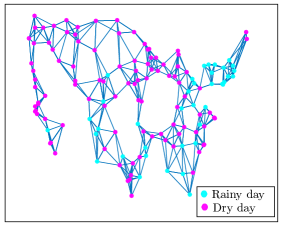
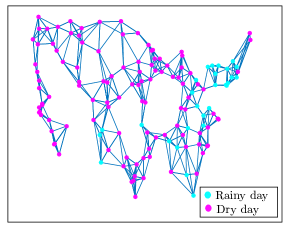
Figure 3: (Left) Occurrence of rain reported by 139 weather stations across the US on July 30, 2015. (Right) Prediction of rain occurrence from weather data based on logistic regression and multitask learning.

TABLE I: Rain prediction error (80) in weather sensor networks for different values of regularization strength $\eta$.

	$\eta=0$	$\eta=10$	$\eta=45$	$\eta=100$	$\eta=1000$	$\eta=\mu^{-1}$
prediction error	0.309	0.232	0.225	0.226	0.228	0.232

V Conclusion

In this work, we considered multitask inference problems where agents in the network have individual parameter vectors to estimate subject to a smoothness condition over the graph. Based on diffusion adaptation, we proposed a strategy that allows the network to minimize a global cost consisting of the aggregate sum of the individual costs regularized by a term promoting smoothness. We showed that, for small step-size parameter, the network is able to approach the minimizer of the regularized problem to arbitrarily good accuracy levels. Furthermore, we showed how the regularization strength can steer the convergence point of the network toward many modes starting from the non-cooperative mode and ending with the single-task mode.

Appendix A Proof of Lemma 1

Consider the matrix inversion identity [38]:

$$(A+BCD)^{-1}=A^{-1}-A^{-1}B(C^{-1}+DA^{-1}B)^{-1}DA^{-1},$$ (81)

which allows us to write:

$$(U+W)^{-1}U=I-U^{-1}(I+WU^{-1})^{-1}W=I-(U+W)^{-1}W,$$ (82)

for any invertible matrix $U$. Using (82), we write (20) alternatively as:

$$\overline{{\scriptstyle\mathcal{W}}}^{o}_{\eta}=\left(I-\eta\left(\overline{\mathcal{H}}_{\eta}^{o}+\eta\mathcal{J}\right)^{-1}\mathcal{J}\right)\overline{{\scriptstyle\mathcal{W}}}^{o}.$$ (83)

Let

$$\mathcal{Q}\triangleq\overline{\mathcal{H}}^{o}_{\eta}+\eta\mathcal{J}.$$ (84)

Using the definitions (21) and (22), we can partition $\mathcal{Q}$ into blocks:

$$\mathcal{Q}=\left[\begin{array}[]{cc}\mathcal{Q}_{11}&\mathcal{Q}_{12}\\ \mathcal{Q}_{12}^{\top}&\mathcal{Q}_{22}\end{array}\right],$$ (85)

with $Q_{11}$, $\mathcal{Q}_{12}$, and $\mathcal{Q}_{22}$ defined in (25), (26), and (27), respectively. Since $v_{1}=\frac{1}{\sqrt{N}}\mathds{1}_{N}$, we have $\mathcal{Q}_{11}=\frac{1}{N}\sum_{k=1}^{N}H^{o}_{k,\eta}$ which is positive definite from Assumption 1. Observe that $\mathcal{Q}$ is invertible since it is similar to $\mathcal{H}^{o}_{\eta}+\eta\mathcal{L}$ which is positive definite under Assumption 1. Now, by applying the block inversion formula to $\mathcal{Q}$, we obtain:

$$\mathcal{Q}^{-1} =(\overline{\mathcal{H}}^{o}_{\eta}+\eta\mathcal{J})^{-1}$$

$$=\left[\begin{array}[]{cc}\mathcal{Q}_{11}^{-1}+\mathcal{Q}_{11}^{-1}\mathcal{Q}_{12}\mathcal{G}\mathcal{Q}_{12}^{\top}\mathcal{Q}_{11}^{-1}&-\mathcal{Q}_{11}^{-1}\mathcal{Q}_{12}\mathcal{G}\\ -\mathcal{G}\mathcal{Q}_{12}^{\top}\mathcal{Q}_{11}^{-1}&\mathcal{G}\end{array}\right],$$ (88)

where

$$\mathcal{G}\triangleq(\mathcal{Q}_{22}-\mathcal{Q}_{12}^{\top}\mathcal{Q}_{11}^{-1}\mathcal{Q}_{12})^{-1}.$$ (89)

Replacing (A) into (83) and using (21), we arrive at:

$$\overline{{\scriptstyle\mathcal{W}}}^{o}_{\eta}=\left[\begin{array}[]{cc}I_{M}&\eta\mathcal{Q}_{11}^{-1}\mathcal{Q}_{12}\mathcal{G}\left(\Lambda_{o}\otimes I_{M}\right)\\ 0&I_{M(N-1)}-\eta\,\mathcal{G}\left(\Lambda_{o}\otimes I_{M}\right)\end{array}\right]\overline{{\scriptstyle\mathcal{W}}}^{o}.$$ (90)

Using definition (29) into (90), we conclude (24).

Now, we establish (30). Let us first introduce the matrix $\mathcal{G}^{\prime}$:

$$\mathcal{G}^{\prime}\triangleq(V_{R}^{\top}\otimes I_{M})\mathcal{H}_{\eta}^{o}(V_{R}\otimes I_{M})-\mathcal{Q}_{12}^{\top}\mathcal{Q}_{11}^{-1}\mathcal{Q}_{12}.$$ (91)

Using the above definition and expressions (28) and (27), we can re-write the matrix $\mathcal{K}$ in (29) alternatively as:

$$\mathcal{K} ={I_{M(N-1)}-\eta\,((V_{R}^{\top}\otimes I_{M})\mathcal{H}^{o}_{\eta}(V_{R}\otimes I_{M})+\eta\Lambda_{o}\otimes I_{M}-\mathcal{Q}_{12}^{\top}\mathcal{Q}_{11}^{-1}\mathcal{Q}_{12})^{-1}\left(\Lambda_{o}\otimes I_{M}\right)}$$

$$={I_{M(N-1)}-\eta(\mathcal{G}^{\prime}+\eta\Lambda_{o}\otimes I_{M})^{-1}(\Lambda_{o}\otimes I_{M})}$$

$$\overset{\eqref{eq: matrix inversion U+V}}{=}(\mathcal{G}^{\prime}+\eta\Lambda_{o}\otimes I_{M})^{-1}\mathcal{G}^{\prime}.$$ (92)

The matrix $\mathcal{G}^{\prime}$ in (91) is the Schur complement of $\overline{\mathcal{H}}^{o}_{\eta}$ in (22) which can be partitioned as:

$$\overline{\mathcal{H}}^{o}_{\eta}=\left[\begin{array}[]{cc}\mathcal{Q}_{11}&\mathcal{Q}_{12}\\ \mathcal{Q}_{12}^{\top}&(V_{R}^{\top}\otimes I_{M})\mathcal{H}^{o}_{\eta}(V_{R}\otimes I_{M})\end{array}\right].$$ (93)

Thus, $\mathcal{G}^{\prime}$ is positive definite since it is the Schur complement of the positive definite matrix $\overline{\mathcal{H}}^{o}_{\eta}$ [39, pp. 651]. Since $\mathcal{G}^{\prime}$ is symmetric, from Weyl’s inequality [40, pp. 239] we have:

$$0<\eta\lambda_{2}(L)+\lambda_{\min}(\mathcal{G}^{\prime})\leq\lambda_{\min}(\mathcal{G}^{\prime}+\eta\Lambda_{o}\otimes I_{M})\leq\eta\lambda_{2}(L)+\lambda_{\max}(\mathcal{G}^{\prime}).$$ (94)

Furthermore, since $\mathcal{G}^{\prime}$ is the Schur complement of the positive definite matrix $\overline{\mathcal{H}}^{o}_{\eta}$, we have [41, Theorem 5]:

$$\lambda_{\min}(\mathcal{G}^{\prime})\geq\lambda_{\min}(\overline{\mathcal{H}}^{o}_{\eta})=\lambda_{\min}(\mathcal{H}^{o}_{\eta})\geq\min_{1\leq k\leq N}\lambda_{k,\min},$$ (95)

$$\lambda_{\max}(\mathcal{G}^{\prime})\leq\lambda_{\max}(\overline{\mathcal{H}}^{o}_{\eta})=\lambda_{\max}(\mathcal{H}^{o}_{\eta})\leq\max_{1\leq k\leq N}\lambda_{k,\max}.$$ (96)

Therefore, from (94) and (95), we get:

$$\lambda_{\min}(\mathcal{G}^{\prime}+\eta\Lambda_{o}\otimes I_{M})\geq\eta\lambda_{2}(L)+\min_{1\leq k\leq N}\lambda_{k,\min},$$ (97)

and

$$\lambda_{\max}((\mathcal{G}^{\prime}+\eta\Lambda_{o}\otimes I_{M})^{-1})=\frac{1}{\lambda_{\min}(\mathcal{G}^{\prime}+\eta\Lambda_{o}\otimes I_{M})}\leq\left(\eta\lambda_{2}(L)+\min_{1\leq k\leq N}\lambda_{k,\min}\right)^{-1}.$$ (98)

Since the $2-$induced norm of a positive definite matrix is equal to its maximum eigenvalue, we obtain:

$$\|(\mathcal{G}^{\prime}+\eta\Lambda_{o}\otimes I_{M})^{-1}\|\leq\left(\eta\lambda_{2}(L)+\min_{1\leq k\leq N}\lambda_{k,\min}\right)^{-1}.$$ (99)

From the sub-multiplicative property of the $2-$induced norm and from (92), (99), and (96), we obtain:

$$\|\mathcal{K}\|\leq\|(\mathcal{G}^{\prime}+\eta\Lambda_{o}\otimes I_{M})^{-1}\|\cdot\|\mathcal{G}^{\prime}\|\leq\left(\max_{1\leq k\leq N}\lambda_{k,\max}\right)\left(\eta\lambda_{2}(L)+\min_{1\leq k\leq N}\lambda_{k,\min}\right)^{-1}.$$ (100)

Appendix B Proof of Lemma 2

Given any two input vectors ${\scriptstyle\mathcal{X}}^{1}$ and ${\scriptstyle\mathcal{X}}^{2}$ with corresponding updated vectors ${\scriptstyle\mathcal{Y}}^{1}$ and ${\scriptstyle\mathcal{Y}}^{2}$, we have from (39):

$${\scriptstyle\mathcal{Y}}^{1}-{\scriptstyle\mathcal{Y}}^{2}=\left(I_{MN}-\mu\eta\mathcal{L}\right)\left({\scriptstyle\mathcal{X}}^{1}-{\scriptstyle\mathcal{X}}^{2}-\mu\,\text{col}\left\{\nabla_{w_{k}}J_{k}(x^{1}_{k})-\nabla_{w_{k}}J_{k}(x^{2}_{k})\right\}_{k=1}^{N}\right).$$ (101)

From the mean-value theorem [33, pp. 24], we have:

$$\nabla_{w_{k}}J_{k}(x^{1}_{k})-\nabla_{w_{k}}J_{k}(x^{2}_{k})=\left(\int_{0}^{1}\nabla^{2}_{w_{k}}J_{k}(x^{2}_{k}+t(x^{1}_{k}-x^{2}_{k}))dt\right)(x^{1}_{k}-x^{2}_{k}).$$ (102)

Using (102) into (101), and the sub-multiplicative property of the $2-$induced norm [7], we obtain:

$$\|{\scriptstyle\mathcal{Y}}^{1}-{\scriptstyle\mathcal{Y}}^{2}\|\leq\|I_{MN}-\mu\eta\mathcal{L}\|\|\mathcal{D}\|\|{\scriptstyle\mathcal{X}}^{1}-{\scriptstyle\mathcal{X}}^{2}\|,$$ (103)

where

$$\mathcal{D}\triangleq\text{diag}\left\{I_{M}-\mu\int_{0}^{1}\nabla^{2}_{w_{k}}J_{k}(x^{2}_{k}+t(x^{1}_{k}-x^{2}_{k}))dt\right\}_{k=1}^{N}.$$ (104)

We have

$$\|I_{MN}-\mu\eta\mathcal{L}\|=\|(I_{N}-\mu\eta L)\otimes I_{M}\|=\|I_{N}-\mu\eta L\|.$$ (105)

Let $\rho(\cdot)$ denote the spectral radius of its matrix argument. Since $L$ is symmetric, we have $\|I_{N}-\mu\eta L\|=\rho(I_{N}-\mu\eta L)$. Since $L$ has one eigenvalue at zero, $\rho(I_{N}-\mu\eta L)$ is guaranteed to be equal to 1 if $\mu\eta$ satisfies condition (36). For the block diagonal symmetric matrix $\mathcal{D}$ in (104), we have:

$$\|\mathcal{D}\|=\max_{1\leq k\leq N}\left\|I_{M}-\mu\int_{0}^{1}\nabla^{2}_{w_{k}}J_{k}(x^{2}_{k}+t(x^{1}_{k}-x^{2}_{k}))dt\right\|.$$ (106)

Due to Assumption 1, we have:

$$0<\lambda_{k,\min}I_{M}\leq\int_{0}^{1}\nabla^{2}_{w_{k}}J_{k}(x^{2}_{k}+t(x^{1}_{k}-x^{2}_{k}))dt\leq\lambda_{k,\max}I_{M}.$$ (107)

It follows that $\|\mathcal{D}\|\leq\gamma$ where $\gamma\triangleq\max_{1\leq k\leq N}\{\gamma_{k}\}$ and $\gamma_{k}$ is given in (41). It holds that $0<\gamma_{k}<1$ when $\mu$ is chosen according to (42). Combining the previous results, we arrive at:

$$\|{\scriptstyle\mathcal{Y}}^{1}-{\scriptstyle\mathcal{Y}}^{2}\|_{2}\leq\gamma\|{\scriptstyle\mathcal{X}}^{1}-{\scriptstyle\mathcal{X}}^{2}\|_{2},$$ (108)

for $\gamma<1$ when (36) and (42) are satisfied and, in this case, the deterministic mapping (39) is a contraction.

Appendix C Proof of Theorem 1

From (49), we obtain the following expression for $\widetilde{\scriptstyle\mathcal{W}}_{\infty}$:

$$\widetilde{\scriptstyle\mathcal{W}}_{\infty}=\mu\eta^{2}[\mathcal{H}_{\infty}+\eta\mathcal{L}-\mu\eta\mathcal{L}\mathcal{H}_{\infty}]^{-1}\mathcal{L}^{2}{\scriptstyle\mathcal{W}}^{o}_{\eta}.$$ (109)

Pre-multiplying both sides of (109) by $\mathcal{V}^{\top}=V^{\top}\otimes I_{M}$ gives:

$$\overline{{\scriptstyle\mathcal{W}}}_{\infty}=\mu\eta^{2}\left[\overline{\mathcal{H}}_{\infty}+\eta\mathcal{J}-\mu\eta\mathcal{J}\overline{\mathcal{H}}_{\infty}\right]^{-1}\mathcal{J}^{2}\,\overline{{\scriptstyle\mathcal{W}}}^{o}_{\eta},$$ (110)

where $\overline{{\scriptstyle\mathcal{W}}}_{\infty}\triangleq\mathcal{V}^{\top}\widetilde{\scriptstyle\mathcal{W}}_{\infty}$, $\overline{{\scriptstyle\mathcal{W}}}^{o}_{\eta}\triangleq\mathcal{V}^{\top}{\scriptstyle\mathcal{W}}^{o}_{\eta}$,

$$\overline{\mathcal{H}}_{\infty}\triangleq\mathcal{V}^{\top}\mathcal{H}_{\infty}\mathcal{V},$$ (111)

and $\mathcal{J}$ is given by (21).

In the following we show that $\overline{{\scriptstyle\mathcal{W}}}_{\infty}$ can be written as:

$$\overline{{\scriptstyle\mathcal{W}}}_{\infty}=\mu\eta^{2}\left[\begin{array}[]{c}-\mathcal{P}_{11}^{-1}\mathcal{P}_{12}\mathcal{T}\\ \mathcal{T}\end{array}\right](\Lambda_{o}^{2}\otimes I_{M})\mathcal{K}[\overline{{\scriptstyle\mathcal{W}}}^{o}]_{2:N},$$ (112)

where $\mathcal{K}$ is defined in (29) and:

$$\mathcal{T} \triangleq(\mathcal{P}_{22}-\mathcal{P}_{21}\mathcal{P}_{11}^{-1}\mathcal{P}_{12})^{-1},$$ (113)

$$\mathcal{P}_{11} \triangleq(v_{1}^{\top}\otimes I_{M})\mathcal{H}_{\infty}(v_{1}\otimes I_{M}){=\frac{1}{N}\sum_{k=1}^{N}H_{k,\infty}},$$ (114)

$$\mathcal{P}_{12} \triangleq(v_{1}^{\top}\otimes I_{M})\mathcal{H}_{\infty}(V_{R}\otimes I_{M}),$$ (115)

$$\mathcal{P}_{21} \triangleq((I_{N-1}-\mu\eta\Lambda_{o})\otimes I_{M})(V_{R}^{\top}\otimes I_{M})\mathcal{H}_{\infty}(v_{1}\otimes I_{M}),$$ (116)

$$\mathcal{P}_{22} \triangleq\eta\Lambda_{o}\otimes I_{M}+((I_{N-1}-\mu\eta\Lambda_{o})\otimes I_{M})(V_{R}^{\top}\otimes I_{M})\mathcal{H}_{\infty}(V_{R}\otimes I_{M}),$$ (117)

We introduce the following matrix, which appears in (110):

$$\mathcal{P}\triangleq(I_{MN}-\mu\eta\mathcal{J})\overline{\mathcal{H}}_{\infty}+\eta\mathcal{J}=\left[\begin{array}[]{cc}\mathcal{P}_{11}&\mathcal{P}_{12}\\ \mathcal{P}_{21}&\mathcal{P}_{22}\end{array}\right],$$ (118)

where the blocks $\{\mathcal{P}_{ij}\}$ are given by (114)–(117). Note that, under Assumption 1, $\mathcal{P}_{11}$ in (114) is invertible since it can be bounded as follows:

$$0<\frac{1}{N}\left(\sum_{k=1}^{N}\lambda_{k,\min}\right)I_{M}\leq\mathcal{P}_{11}\leq\frac{1}{N}\left(\sum_{k=1}^{N}\lambda_{k,\max}\right)I_{M}.$$ (119)

Applying the block inversion formula to $\mathcal{P}$, we obtain:

$$\mathcal{P}^{-1}=\left[\begin{array}[]{cc}\mathcal{P}_{11}^{-1}+\mathcal{P}_{11}^{-1}\mathcal{P}_{12}\mathcal{T}\mathcal{P}_{21}\mathcal{P}_{11}^{-1}&-\mathcal{P}_{11}^{-1}\mathcal{P}_{12}\mathcal{T}\\ -\mathcal{T}\mathcal{P}_{21}\mathcal{P}_{11}^{-1}&\mathcal{T}\end{array}\right],$$ (120)

with $\mathcal{T}$ defined in (113). Replacing (120) into (110), and using (21) and (24), we conclude (112).

Our goal now is to show that

$$\lim_{\mu\rightarrow 0}\frac{\|{\scriptstyle\mathcal{W}}^{o}_{\eta}-{\scriptstyle\mathcal{W}}_{\infty}\|}{\mu}=c,$$ (121)

for some constant $c$ that may depend on $\eta$ (the regularization strength), but not on $\mu$ (the step-size parameter). From (112), we have:

$$\lim_{\mu\rightarrow 0}\frac{\|{\scriptstyle\mathcal{W}}^{o}_{\eta}-{\scriptstyle\mathcal{W}}_{\infty}\|}{\mu}=\eta^{2}\lim_{\mu\rightarrow 0}\left\|\left[\begin{array}[]{c}-\mathcal{P}_{11}^{-1}\mathcal{P}_{12}\mathcal{T}\\ \mathcal{T}\end{array}\right](\Lambda_{o}^{2}\otimes I_{M})\mathcal{K}[\overline{{\scriptstyle\mathcal{W}}}^{o}]_{2:N}\right\|.$$ (122)

Since the Euclidean norm is continuous, we have $\lim_{\mu\rightarrow 0}\|g(\mu)\|=\|\lim_{\mu\rightarrow 0}g(\mu)\|$. In the following we show that

$$\eta^{4}\left\|\lim_{\mu\rightarrow 0}\mathcal{T}(\Lambda_{o}^{2}\otimes I_{M})\mathcal{K}[\overline{{\scriptstyle\mathcal{W}}}^{o}]_{2:N}\right\|^{2}\leq{O(\eta^{4})(O(1)+O(\eta))^{-4}},$$ (123)

and

$$\eta^{4}\left\|\lim_{\mu\rightarrow 0}\mathcal{P}_{11}^{-1}\mathcal{P}_{12}\mathcal{T}(\Lambda_{o}^{2}\otimes I_{M})\mathcal{K}[\overline{{\scriptstyle\mathcal{W}}}^{o}]_{2:N}\right\|^{2}\leq O(\eta^{4})(O(1)+O(\eta))^{-4}.$$ (124)

From (122), (123), and (124), we can conclude (52).

Let us first establish (123). We have:

$$\|\mathcal{T}(\Lambda_{o}^{2}\otimes I_{M})\mathcal{K}[\overline{{\scriptstyle\mathcal{W}}}^{o}]_{2:N}\|^{2}\leq\|\mathcal{T}\|^{2}\|\Lambda_{o}^{2}\|^{2}\|\mathcal{K}\|^{2}\|[\overline{{\scriptstyle\mathcal{W}}}^{o}]_{2:N}\|^{2}.$$ (125)

From (30), we have $\|\mathcal{K}\|^{2}\leq(O(1)+O(\eta))^{-2}$. For sufficiently small step-sizes, we have:

$$\lim_{\mu\rightarrow 0}\mathcal{P}_{21}=(V_{R}^{\top}\otimes I_{M})\mathcal{H}_{\infty}(v_{1}\otimes I_{M}),$$ (126)

$$\lim_{\mu\rightarrow 0}\mathcal{P}_{22}=\eta\Lambda_{o}\otimes I_{M}+(V_{R}^{\top}\otimes I_{M})\mathcal{H}_{\infty}(V_{R}\otimes I_{M}).$$ (127)

Following the same line of reasoning as in (91)–(99), we can show that, when $\mu\rightarrow 0$, we have:

$$\|\mathcal{T}\|^{2}\leq\left(\eta\lambda_{2}(L)+\min_{1\leq k\leq N}\lambda_{k,\min}\right)^{-2}=(O(1)+O(\eta))^{-2}.$$ (128)

Thus, we conclude (123).

Now, we establish (124). From (119), we have $\mathcal{P}_{11}=O(1)$ and $\|\mathcal{P}_{11}^{-1}\|^{2}=O(1)$. Similarly, we can conclude from (115) that $\|\mathcal{P}_{12}\|^{2}\leq O(1)$. Thus, using (123), we arrive at (124).

Appendix D Proof of Theorem 2

From (6), (35), and (44), we have:

$${\scriptstyle\mathcal{W}}_{\infty}-\boldsymbol{{\scriptstyle\mathcal{W}}}_{i}=(I_{MN}-\mu\eta\mathcal{L})\left({\scriptstyle\mathcal{W}}_{\infty}-\boldsymbol{{\scriptstyle\mathcal{W}}}_{i-1}-\mu\,\text{col}\left\{\nabla_{w_{k}}J_{k}(w_{k,\infty})-\nabla_{w_{k}}J_{k}(\boldsymbol{w}_{k,i-1})\right\}_{k=1}^{N}-\mu\,\text{col}\left\{\boldsymbol{s}_{k,i}(\boldsymbol{w}_{k,i-1})\right\}_{k=1}^{N}\right).$$ (129)

Using the mean-value theorem (102), the above relation can be written as:

$${\scriptstyle\mathcal{W}}_{\infty}-\boldsymbol{{\scriptstyle\mathcal{W}}}_{i}=(I_{MN}-\mu\eta\mathcal{L})\left((I_{MN}-\mu\boldsymbol{\cal{H}}_{i-1})({\scriptstyle\mathcal{W}}_{\infty}-\boldsymbol{{\scriptstyle\mathcal{W}}}_{i-1})-\mu\,\text{col}\{\boldsymbol{s}_{k,i}(\boldsymbol{w}_{k,i-1})\}_{k=1}^{N}\right),$$ (130)

where $\boldsymbol{\cal{H}}_{i-1}\triangleq\text{diag}\{\boldsymbol{H}_{1,i-1},\ldots,\boldsymbol{H}_{N,i-1}\}$ with:

$$\boldsymbol{H}_{k,i-1}\triangleq\int_{0}^{1}\nabla^{2}_{w_{k}}J_{k}(w_{k,\infty}-t(w_{k,\infty}-\boldsymbol{w}_{k,i-1}))dt$$ (131)

Let

$$\boldsymbol{\phi}_{i} \triangleq(I_{MN}-\mu\boldsymbol{\cal{H}}_{i-1})({\scriptstyle\mathcal{W}}_{\infty}-\boldsymbol{{\scriptstyle\mathcal{W}}}_{i-1})-\mu\,\text{col}\{\boldsymbol{s}_{k,i}(\boldsymbol{w}_{k,i-1})\}_{k=1}^{N}$$ (132)

$$C \triangleq I_{N}-\mu\eta L.$$ (133)

From the Laplacian matrix definition, it can be verified that the off-diagonal entries of the matrix $C$ are non-negative and that its diagonal entries are non-negative under condition (37). Furthermore, since we have $L\mathds{1}_{N}=0$, the entries on each row of $C$ will add up to one. Thus, applying Jensen’s inequality [39, pp. 77] to the convex function $\|\cdot\|^{2}$, we obtain from (130) and (132):

$$\mathbb{E}\|w_{k,\infty}-\boldsymbol{w}_{k,i}\|^{2}\leq\sum_{\ell=1}^{N}[C]_{k\ell}\mathbb{E}\|\boldsymbol{\phi}_{\ell,i}\|^{2},$$ (134)

where $\boldsymbol{\phi}_{k,i}$ is the $k$-th sub-vector of $\boldsymbol{\phi}_{i}$ given by:

$$\boldsymbol{\phi}_{k,i}=(I_{M}-\mu\boldsymbol{H}_{k,i-1})(w_{k,\infty}-\boldsymbol{w}_{k,i-1})-\mu\boldsymbol{s}_{k,i}(\boldsymbol{w}_{k,i-1}).$$ (135)

Squaring both sides of (135), conditioning on $\boldsymbol{\cal{F}}_{i-1}$, and taking expectations we obtain:

$$\begin{split}\mathbb{E}[\|\boldsymbol{\phi}_{k,i}\|^{2}|\boldsymbol{\cal{F}}_{i-1}]&=\|w_{k,\infty}-\boldsymbol{w}_{k,i-1}\|^{2}_{\boldsymbol{\Sigma}_{k,i-1}}+\mu^{2}\mathbb{E}[\|\boldsymbol{s}_{k,i}(\boldsymbol{w}_{k,i-1})\|^{2}|\boldsymbol{\cal{F}}_{i-1}].\end{split}$$ (136)

where $\boldsymbol{\Sigma}_{k,i-1}\triangleq(I_{M}-\mu\boldsymbol{H}_{k,i-1})^{2}$ and where the cross term is zero because of the zero-mean condition (32). Due to Assumption 1, $\boldsymbol{\Sigma}_{k,i-1}$ can be bounded as follows:

$$0<\boldsymbol{\Sigma}_{k,i-1}\leq\gamma_{k}^{2}I_{M},$$ (137)

where $\gamma_{k}$ is given by (41). From Assumption 2, $\mathbb{E}[\|\boldsymbol{s}_{k,i}(\boldsymbol{w}_{k,i-1})\|^{2}|\boldsymbol{\cal{F}}_{i-1}]$ can be bounded as follows:

$$\mathbb{E}[\|\boldsymbol{s}_{k,i}(\boldsymbol{w}_{k,i-1})\|^{2}|\boldsymbol{\cal{F}}_{i-1}] \leq\beta_{k}^{2}\|\boldsymbol{w}_{k,i-1}\|^{2}+\sigma^{2}_{s,k}$$

$$=\beta_{k}^{2}\|w^{o}_{k,\eta}-w_{k,\infty}+w_{k,\infty}-\boldsymbol{w}_{k,i-1}-w^{o}_{k,\eta}\|^{2}+\sigma^{2}_{s,k}$$

$$\leq 3\beta_{k}^{2}\|w^{o}_{k,\eta}-w_{k,\infty}\|^{2}+3\beta_{k}^{2}\|w_{k,\infty}-\boldsymbol{w}_{k,i-1}\|^{2}+3\beta_{k}^{2}\|w^{o}_{k,\eta}\|^{2}+\sigma^{2}_{s,k}.$$ (138)

Taking expectation again in (136), and using the bounds (137) and (138), we obtain:

$$\mathbb{E}\|\boldsymbol{\phi}_{k,i}\|^{2} =\mathbb{E}\|w_{k,\infty}-\boldsymbol{w}_{k,i-1}\|^{2}_{\boldsymbol{\Sigma}_{k,i-1}}+\mu^{2}\mathbb{E}\|\boldsymbol{s}_{k,i}(\boldsymbol{w}_{k,i-1})\|^{2}$$

$$\leq(\gamma_{k}^{2}+3\mu^{2}\beta^{2}_{k})\mathbb{E}\|w_{k,\infty}-\boldsymbol{w}_{k,i-1}\|^{2}+\mu^{2}\left(3\beta_{k}^{2}\|w^{o}_{k,\eta}-w_{k,\infty}\|^{2}+3\beta_{k}^{2}\|w^{o}_{k,\eta}\|^{2}+\sigma^{2}_{s,k}\right).$$ (139)

Now, combining (139) and (134), we obtain (54).

Iterating (54) starting from $i=1$, we get:

$$\text{MSP}_{i}\preceq(CG)^{i}\text{MSP}_{0}+\mu^{2}\sum_{j=0}^{i-1}(CG)^{j}Cb.$$ (140)

Under Assumption 3 and condition (57), the matrix $CG$ can be guaranteed to be stable. To see this, we upper bound the spectral radius as follows:

$$\rho(CG)\leq\|CG\|_{\infty}\leq\|C\|_{\infty}\|G\|_{\infty}=\|G\|_{\infty}=\max_{1\leq k\leq N}\gamma_{k}^{2}+3\mu^{2}\beta_{k}^{2},$$ (141)

where we used the fact that, under condition (37), the matrix $C$ is a right-stochastic matrix. We have:

$$\gamma_{k}^{2}+3\mu^{2}\beta_{k}^{2}=\max\{1-2\mu\lambda_{k,\min}+\mu^{2}\lambda_{k,\min}^{2}+3\mu^{2}\beta_{k}^{2},1-2\mu\lambda_{k,\max}+\mu^{2}\lambda_{k,\max}^{2}+3\mu^{2}\beta_{k}^{2}\},$$ (142)

which is guaranteed to be less than one when:

$$0<\mu<\min\left\{\frac{2\lambda_{k,\min}}{\lambda_{k,\min}^{2}+3\beta_{k}^{2}},\frac{2\lambda_{k,\max}}{\lambda_{k,\max}^{2}+3\beta_{k}^{2}}\right\}.$$ (143)

Then we conclude that the matrix $CG$ is stable under condition (57). In this case, we have:

$$\limsup_{i\rightarrow\infty}\text{MSP}_{i}\preceq\mu^{2}\sum_{j=0}^{\infty}(CG)^{j}Cb.$$ (144)

Using the submultiplicative property of the induced infinity norm, we obtain:

$$\begin{split}\|\limsup_{i\rightarrow\infty}\text{MSP}_{i}\|_{\infty}&\leq\mu^{2}\left\|\sum_{j=0}^{\infty}(CG)^{j}\right\|_{\infty}\|C\|_{\infty}\|b\|_{\infty}\\ &\leq\mu^{2}\sum_{j=0}^{\infty}\|(CG)^{j}\|_{\infty}\|b\|_{\infty},\\ &\leq\mu^{2}\sum_{j=0}^{\infty}\|C\|^{j}_{\infty}\|G\|_{\infty}^{j}\|b\|_{\infty}=\frac{\mu^{2}\|b\|_{\infty}}{1-\|G\|_{\infty}},\end{split}$$ (145)

where we used the fact that $\|C\|_{\infty}=1$ and where $\|G\|_{\infty}=\max_{1\leq k\leq N}\gamma_{k}^{2}+3\mu^{2}\beta_{k}^{2}$. From (142), we have:

$$\gamma_{k}^{2}+3\mu^{2}\beta_{k}^{2}=1-\mu\zeta_{k},$$ (146)

where

$$\zeta_{k}\triangleq\min\{2\lambda_{k,\min}-\mu\lambda_{k,\min}^{2}-3\mu\beta_{k}^{2},2\lambda_{k,\max}-\mu\lambda_{k,\max}^{2}-3\mu\beta_{k}^{2}\}.$$ (147)

Thus,

$$\|G\|_{\infty}=\max_{1\leq k\leq N}\{1-\mu\zeta_{k}\}=1-\mu\min_{1\leq k\leq N}\zeta_{k}.$$ (148)

Substituting into (145), we obtain:

$$\|\limsup_{i\rightarrow\infty}\text{MSP}_{i}\|_{\infty}\leq\frac{\mu\|b\|_{\infty}}{\min_{1\leq k\leq N}\zeta_{k}}.$$ (149)

For sufficiently small $\mu$, we have from (56) and Theorem 1 that $\|b\|=O(1)+O(\mu^{2}\eta^{4})(O(1)+O(\eta))^{-4}$. We conclude that $\|\limsup_{i\rightarrow\infty}\text{MSP}_{i}\|_{\infty}{\leq}O(\mu)$.

From (43), we have:

$$\limsup_{i\rightarrow\infty}\mathbb{E}\|{\scriptstyle\mathcal{W}}^{o}_{\eta}-\boldsymbol{{\scriptstyle\mathcal{W}}}_{i}\|^{2} \leq 2\|{\scriptstyle\mathcal{W}}^{o}_{\eta}-{\scriptstyle\mathcal{W}}_{\infty}\|^{2}+2\limsup_{i\rightarrow\infty}\mathds{1}_{N}^{\top}\cdot\text{MSP}_{i}$$ (150)

Therefore, from Theorem 1 and (58), we conclude (59).

Appendix E Proof of Theorem 3

Applying Jensen’s inequality [39, pp. 77] to the convex function $\|\cdot\|^{4}$, we obtain from (130) and (132):

$$\mathbb{E}\|w_{k,\infty}-\boldsymbol{w}_{k,i}\|^{4}\leq\sum_{\ell=1}^{N}[C]_{k\ell}\mathbb{E}\|\boldsymbol{\phi}_{\ell,i}\|^{4},$$ (151)

where $C$ and $\boldsymbol{\phi}_{k,i}$ are given by (133) and (135), respectively. Using the inequality [7, pp. 523]:

$$\|a+b\|^{4}\leq\|a\|^{4}+3\|b\|^{4}+8\|a\|^{2}\|b\|^{2}+4\|a\|^{2}(a^{\top}b),$$ (152)

we obtain from (135) under Assumption 2 on the gradient noise:

$$\begin{split}\mathbb{E}\|\boldsymbol{\phi}_{k,i}\|^{4}\leq&~{}\mathbb{E}\|(I_{M}-\mu\boldsymbol{H}_{k,i-1})(w_{k,\infty}-\boldsymbol{w}_{k,i-1})\|^{4}+3\mu^{4}\mathbb{E}\|\boldsymbol{s}_{k,i}(\boldsymbol{w}_{k,i-1})\|^{4}+\\ &\quad 8\mu^{2}\left(\mathbb{E}\|(I_{M}-\mu\boldsymbol{H}_{k,i-1})(w_{k,\infty}-\boldsymbol{w}_{k,i-1})\|^{2}\right)\left(\mathbb{E}\|\boldsymbol{s}_{k,i}(\boldsymbol{w}_{k,i-1})\|^{2}\right).\end{split}$$ (153)

From Assumption 1, the matrices $(I_{M}-\mu\boldsymbol{H}_{k,i-1})^{2}$ and $(I_{M}-\mu\boldsymbol{H}_{k,i-1})^{4}$ can be bounded as follows:

$$0<(I_{M}-\mu\boldsymbol{H}_{k,i-1})^{2}\leq\gamma_{k}^{2}I_{M},$$ (154)

$$0<(I_{M}-\mu\boldsymbol{H}_{k,i-1})^{4}\leq\gamma_{k}^{4}I_{M},$$ (155)

where $\gamma_{k}$ is given by (41). Thus, we obtain:

$$\mathbb{E}\|\boldsymbol{\phi}_{k,i}\|^{4}\leq\gamma_{k}^{4}\mathbb{E}\|w_{k,\infty}-\boldsymbol{w}_{k,i-1}\|^{4}+3\mu^{4}\mathbb{E}\|\boldsymbol{s}_{k,i}(\boldsymbol{w}_{k,i-1})\|^{4}+8\mu^{2}\gamma_{k}^{2}\left(\mathbb{E}\|w_{k,\infty}-\boldsymbol{w}_{k,i-1}\|^{2}\right)\left(\mathbb{E}\|\boldsymbol{s}_{k,i}(\boldsymbol{w}_{k,i-1})\|^{2}\right).$$ (156)

Under condition (60), we have:

$$\mathbb{E}\left[\|\boldsymbol{s}_{k,i}(\boldsymbol{w}_{k,i-1})\|^{4}|\boldsymbol{\cal{F}}_{i-1}\right] \leq\overline{\beta}_{k}^{4}\|\boldsymbol{w}_{k,i-1}\|^{4}+\overline{\sigma}^{4}_{s,k}$$

$$=\overline{\beta}_{k}^{4}\|w^{o}_{k,\eta}-w_{k,\infty}+w_{k,\infty}-\boldsymbol{w}_{k,i-1}-w^{o}_{k,\eta}\|^{4}+\overline{\sigma}^{4}_{s,k}$$

$$\leq 27\overline{\beta}_{k}^{4}\|w^{o}_{k,\eta}-w_{k,\infty}\|^{4}+27\overline{\beta}_{k}^{4}\|w_{k,\infty}-\boldsymbol{w}_{k,i-1}\|^{4}+27\overline{\beta}_{k}^{4}\|w^{o}_{k,\eta}\|^{4}+\overline{\sigma}^{4}_{s,k},$$ (157)

where we applied Jensen’s inequality to the function $\|\cdot\|^{4}$. Furthermore, from (138), the last term on the RHS of (156) can be bounded as follows:

$$\left(\mathbb{E}\|w_{k,\infty}-\boldsymbol{w}_{k,i-1}\|^{2}\right)\left(\mathbb{E}\|\boldsymbol{s}_{k,i}(\boldsymbol{w}_{k,i-1})\|^{2}\right)$$

$$\leq 3\beta_{k}^{2}\left(\mathbb{E}\|w_{k,\infty}-\boldsymbol{w}_{k,i-1}\|^{2}\right)^{2}+\left(3\beta_{k}^{2}\|w^{o}_{k,\eta}-w_{k,\infty}\|^{2}+3\beta_{k}^{2}\|w^{o}_{k,\eta}\|^{2}+\sigma^{2}_{s,k}\right)\mathbb{E}\|w_{k,\infty}-\boldsymbol{w}_{k,i-1}\|^{2}$$

$$\leq 3\beta_{k}^{2}\mathbb{E}\|w_{k,\infty}-\boldsymbol{w}_{k,i-1}\|^{4}+\left(3\beta_{k}^{2}\|w^{o}_{k,\eta}-w_{k,\infty}\|^{2}+3\beta_{k}^{2}\|w^{o}_{k,\eta}\|^{2}+\sigma^{2}_{s,k}\right)\mathbb{E}\|w_{k,\infty}-\boldsymbol{w}_{k,i-1}\|^{2},$$ (158)

where we used the fact that for any random variable $\boldsymbol{a}$, we have $(\mathbb{E}\boldsymbol{a})^{2}\leq\mathbb{E}\boldsymbol{a}^{2}$. Replacing (157) and (158) into (156), we obtain:

$$\begin{split}\mathbb{E}\|\boldsymbol{\phi}_{k,i}\|^{4}\leq&~{}(\gamma_{k}^{4}+81\mu^{4}\overline{\beta}_{k}^{4}+24\mu^{2}\gamma_{k}^{2}\beta_{k}^{2})\mathbb{E}\|w_{k,\infty}-\boldsymbol{w}_{k,i-1}\|^{4}+\\ &~{}8\mu^{2}\gamma_{k}^{2}(3\beta_{k}^{2}\|w^{o}_{k,\eta}-w_{k,\infty}\|^{2}+3\beta_{k}^{2}\|w^{o}_{k,\eta}\|^{2}+\sigma^{2}_{s,k})\mathbb{E}\|w_{k,\infty}-\boldsymbol{w}_{k,i-1}\|^{2}+\\ &~{}81\mu^{4}\overline{\beta}_{k}^{4}\|w^{o}_{k,\eta}-w_{k,\infty}\|^{4}+81\mu^{4}\overline{\beta}_{k}^{4}\|w^{o}_{k,\eta}\|^{4}+3\mu^{4}\overline{\sigma}^{4}_{s,k}.\end{split}$$ (159)

Now, combining (159) and (151), we arrive at (64).

Iterating (64) starting from $i=1$, we get:

$$\text{MFP}_{i}\preceq(CG^{\prime})^{i}\text{MFP}_{0}+\mu^{2}\sum_{j=0}^{i-1}(CG^{\prime})^{j}CB\text{MSP}_{i-1-j}+\mu^{4}\sum_{j=0}^{i-1}(CG^{\prime})^{j}Cb^{\prime}.$$ (160)

Under Assumption 3 and for sufficiently small $\mu$, the matrix $CG^{\prime}$ can be guaranteed to be stable. To see this, we upper bound its spectral radius as follows:

$$\rho(CG^{\prime})\leq\|CG^{\prime}\|_{\infty}\leq\|C\|_{\infty}\|G^{\prime}\|_{\infty}=\|G^{\prime}\|_{\infty},$$ (161)

since under condition (37), $C$ is a right-stochastic matrix. The $\infty-$norm of $G^{\prime}$ is given by:

$$\|G^{\prime}\|_{\infty} =\max_{1\leq k\leq N}\left\{\gamma_{k}^{4}+24\mu^{2}\gamma_{k}^{2}\beta_{k}^{2}+81\mu^{4}\overline{\beta}_{k}^{4}\right\}$$

$$=\max_{1\leq k\leq N}\big{\{}\max\{1-4\mu\lambda_{k,\min}+6\mu^{2}\lambda_{k,\min}^{2}-4\mu^{3}\lambda_{k,\min}^{3}+\mu^{4}\lambda_{k,\min}^{4}+24\mu^{2}\gamma_{k}^{2}\beta_{k}^{2}+81\mu^{4}\overline{\beta}_{k}^{4},$$

$$~{}\quad\qquad\qquad\qquad 1-4\mu\lambda_{k,\max}+6\mu^{2}\lambda_{k,\max}^{2}-4\mu^{3}\lambda_{k,\max}^{3}+\mu^{4}\lambda_{k,\max}^{4}+24\mu^{2}\gamma_{k}^{2}\beta_{k}^{2}+81\mu^{4}\overline{\beta}_{k}^{4}\}\big{\}}$$

$$=1-\mu\min_{1\leq k\leq N}\big{\{}\min\{4\lambda_{k,\min}-6\mu\lambda_{k,\min}^{2}+4\mu^{2}\lambda_{k,\min}^{3}-\mu^{3}\lambda_{k,\min}^{4}-24\mu\gamma_{k}^{2}\beta_{k}^{2}-81\mu^{3}\overline{\beta}_{k}^{4},$$

$$~{}\quad\qquad\qquad\qquad\qquad 4\lambda_{k,\max}-6\mu\lambda_{k,\max}^{2}+4\mu^{2}\lambda_{k,\max}^{3}-\mu^{3}\lambda_{k,\max}^{4}-24\mu\gamma_{k}^{2}\beta_{k}^{2}-81\mu^{3}\overline{\beta}_{k}^{4}\}\big{\}}.$$ (162)

A sufficiently small $\mu$ ensures $\|G^{\prime}\|_{\infty}<1$ and, thus, ensures the stability of $CG^{\prime}$.

We have established in Theorem 2 that, for small $\mu$, after sufficient iterations have passed, $\text{MSP}_{j}$ converges to a bounded region on the order of $\mu$. This implies that, there exists a $j_{o}$ large enough such that for all $j\geq j_{o}$ it holds that:

$$\|\text{MSP}_{j}\|_{\infty}\leq s_{\max}=O(\mu).$$ (163)

In this case, we have from (160):

$$\limsup_{i\rightarrow\infty}\text{MFP}_{i} \preceq\mu^{4}\sum_{j=0}^{\infty}(CG^{\prime})^{j}Cb^{\prime}+\mu^{2}\limsup_{i\rightarrow\infty}\sum_{j=0}^{i-1}(CG^{\prime})^{j}CB\text{MSP}_{i-1-j}$$

$$=\mu^{4}\sum_{j=0}^{\infty}(CG^{\prime})^{j}Cb^{\prime}+\mu^{2}\limsup_{i\rightarrow\infty}\sum_{j=0}^{i-1}(CG^{\prime})^{i-1-j}CB\text{MSP}_{j}$$

$$=\mu^{4}\sum_{j=0}^{\infty}(CG^{\prime})^{j}Cb^{\prime}+\mu^{2}\limsup_{i\rightarrow\infty}\left(\sum_{j=0}^{j_{o}}(CG^{\prime})^{i-1-j}CB\text{MSP}_{j}+\sum_{j=j_{o}+1}^{i-1}(CG^{\prime})^{i-1-j}CB\text{MSP}_{j}\right)$$

$$=\mu^{4}\sum_{j=0}^{\infty}(CG^{\prime})^{j}Cb^{\prime}+\mu^{2}\limsup_{i\rightarrow\infty}\left((CG^{\prime})^{i}\sum_{j=0}^{j_{o}}(CG^{\prime})^{-1-j}CB\text{MSP}_{j}+\sum_{j=j_{o}+1}^{i-1}(CG^{\prime})^{i-1-j}CB\text{MSP}_{j}\right)$$

$$=\mu^{4}\sum_{j=0}^{\infty}(CG^{\prime})^{j}Cb^{\prime}+\mu^{2}\limsup_{i\rightarrow\infty}\sum_{j=j_{o}+1}^{i-1}(CG^{\prime})^{i-1-j}CB\text{MSP}_{j}.$$ (164)

Using the submultiplicative and sub-additive properties of the induced infinity norm, we obtain:

$$\|\limsup_{i\rightarrow\infty}\text{MFP}_{i}\|_{\infty} \leq\mu^{4}\left\|\sum_{j=0}^{\infty}(CG^{\prime})^{j}\right\|_{\infty}\|b^{\prime}\|_{\infty}+\mu^{2}\limsup_{i\rightarrow\infty}\sum_{j=j_{o}+1}^{i-1}\|(CG^{\prime})^{i-1-j}CB\text{MSP}_{j}\|_{\infty}$$

$$\leq\mu^{4}\sum_{j=0}^{\infty}\|G^{\prime}\|_{\infty}^{j}\|b^{\prime}\|_{\infty}+\mu^{2}\limsup_{i\rightarrow\infty}\sum_{j=0}^{i-j_{o}-2}\|G^{\prime}\|_{\infty}^{j}\|B\|_{\infty}s_{\max}$$

$$=\mu^{4}\frac{\|b^{\prime}\|_{\infty}}{1-\|G^{\prime}\|_{\infty}}+\mu^{2}\frac{\|B\|_{\infty}s_{\max}}{1-\|G^{\prime}\|_{\infty}}$$ (165)

where in the second line we used (163) and where $\|G^{\prime}\|_{\infty}$ is given by (162). Since $\|b^{\prime}\|_{\infty}=O(1)$, $\|B\|_{\infty}=O(1)$, $s_{\max}=O(\mu)$, and $1-\|G^{\prime}\|_{\infty}=O(\mu)$, we conclude (68).

From (61) and (62), we have:

$$\limsup_{i\rightarrow\infty}\mathbb{E}\|{\scriptstyle\mathcal{W}}_{\eta}^{o}-\boldsymbol{{\scriptstyle\mathcal{W}}}_{i}\|^{4}\leq 8\|{\scriptstyle\mathcal{W}}_{\eta}^{o}-{\scriptstyle\mathcal{W}}_{\infty}\|^{4}+8N\limsup_{i\rightarrow\infty}\mathds{1}_{N}\cdot\text{MFP}_{i}.$$ (166)

Therefore, from Theorem 1 and (68), we conclude (69).

Appendix F Proof of Theorem 4

Conditioning both sides of (130), invoking the conditions on the gradient noise from Assumption 2, and computing the conditional expectations, we obtain:

$$\mathbb{E}[({\scriptstyle\mathcal{W}}_{\infty}-\boldsymbol{{\scriptstyle\mathcal{W}}}_{i})|\boldsymbol{\cal{F}}_{i-1}]=(I_{MN}-\mu\eta\mathcal{L})(I_{MN}-\mu\boldsymbol{\cal{H}}_{i-1})({\scriptstyle\mathcal{W}}_{\infty}-\boldsymbol{{\scriptstyle\mathcal{W}}}_{i-1}).$$ (167)

Taking expectations again, we arrive at:

$$\mathbb{E}({\scriptstyle\mathcal{W}}_{\infty}-\boldsymbol{{\scriptstyle\mathcal{W}}}_{i})=(I_{MN}-\mu\eta\mathcal{L})\mathbb{E}[(I_{MN}-\mu\boldsymbol{\cal{H}}_{i-1})({\scriptstyle\mathcal{W}}_{\infty}-\boldsymbol{{\scriptstyle\mathcal{W}}}_{i-1})].$$ (168)

Applying Jensen’s inequality [39, pp. 77] to the convex function $\|\cdot\|^{2}$, we obtain from the above relation:

$$\|\mathbb{E}(w_{k,\infty}-\boldsymbol{w}_{k,i})\|^{2}\leq\sum_{\ell=1}^{N}[C]_{k\ell}\left\|\mathbb{E}\left[(I_{M}-\mu\boldsymbol{H}_{\ell,i-1})(w_{\ell,\infty}-\boldsymbol{w}_{\ell,i-1})\right]\right\|^{2},$$ (169)

where $C$ and $\boldsymbol{H}_{k,i-1}$ are given by (133) and (131), respectively. Let

$$\widetilde{\boldsymbol{H}}_{k,i-1}\triangleq H_{k,\eta}-\boldsymbol{H}_{k,i-1},$$ (170)

where

$$H_{k,\eta}=\nabla_{w_{k}}^{2}J_{k}(w_{k,\eta}^{o}).$$ (171)

Then, we can write:

$$\mathbb{E}\left[(I_{M}-\mu\boldsymbol{H}_{k,i-1})(w_{k,\infty}-\boldsymbol{w}_{k,i-1})\right]=(I_{M}-\mu H_{k,\eta})\mathbb{E}(w_{k,\infty}-\boldsymbol{w}_{k,i-1})+\mu\boldsymbol{c}_{k,i-1},$$ (172)

in terms of a deterministic perturbation sequence defined by

$$\boldsymbol{c}_{k,i-1}\triangleq\mathbb{E}[\widetilde{\boldsymbol{H}}_{k,i-1}(w_{k,\infty}-\boldsymbol{w}_{k,i-1})].$$ (173)

By applying Jensen’s inequality to the convex function $\|\cdot\|^{2}$, we obtain:

$$\|\mathbb{E}(I_{M}-\mu\boldsymbol{H}_{k,i-1})(w_{k,\infty}-\boldsymbol{w}_{k,i-1})\|^{2}$$

$$=\|(I_{M}-\mu H_{k,\eta})\mathbb{E}(w_{k,\infty}-\boldsymbol{w}_{k,i-1})+\mu\boldsymbol{c}_{k,i-1}\|^{2}$$

$$=\left\|t\frac{1}{t}(I_{M}-\mu H_{k,\eta})\mathbb{E}(w_{k,\infty}-\boldsymbol{w}_{k,i-1})+\mu(1-t)\frac{1}{1-t}\boldsymbol{c}_{k,i-1}\right\|^{2}$$

$$\leq t\left\|\frac{1}{t}(I_{M}-\mu H_{k,\eta})\mathbb{E}(w_{k,\infty}-\boldsymbol{w}_{k,i-1})\right\|^{2}+\mu^{2}(1-t)\left\|\frac{1}{1-t}\boldsymbol{c}_{k,i-1}\right\|^{2}$$

$$=\frac{1}{t}\|(I_{M}-\mu H_{k,\eta})\mathbb{E}(w_{k,\infty}-\boldsymbol{w}_{k,i-1})\|^{2}+\mu^{2}\frac{1}{1-t}\|\boldsymbol{c}_{k,i-1}\|^{2},$$ (174)

for any arbitrary positive number $t\in(0,1)$. We select $t=\gamma_{k}$ where $\gamma_{k}$ is given by (41), which is guaranteed to be less than one under condition (42). From Assumption 1, we have $\|I_{M}-\mu H_{k,\eta}\|^{2}\leq\gamma^{2}_{k}$. Thus, we obtain:

$$\|\mathbb{E}(I_{M}-\mu\boldsymbol{H}_{k,i-1})(w_{k,\infty}-\boldsymbol{w}_{k,i-1})\|^{2}\leq\gamma_{k}\|\mathbb{E}(w_{k,\infty}-\boldsymbol{w}_{k,i-1})\|^{2}+\mu^{2}\frac{1}{1-\gamma_{k}}\|\boldsymbol{c}_{k,i-1}\|^{2}.$$ (175)

As shown in [7, Appendix E], the Hessian of a twice differentiable strongly convex function $J_{k}(w_{k})$ satisfying Assumptions 1 and 4 is globally Lipschitz relative to $w^{o}_{k,\eta}$, namely, it satisfies:

$$\|\nabla^{2}_{w_{k}}J_{k}(w_{k})-\nabla^{2}_{w_{k}}J_{k}(w^{o}_{k,\eta})\|\leq\kappa^{\prime}_{d}\|w_{k}-w^{o}_{k,\eta}\|,\quad\forall w_{k},$$ (176)

where $\kappa^{\prime}_{d}=\max\{\kappa_{d},\frac{\lambda_{k,\max}-\lambda_{k,\min}}{\epsilon}\}$. Then, for each agent $k$ we obtain:

$$\|\widetilde{\boldsymbol{H}}_{k,i-1}\| \triangleq\|H_{k,\eta}-\boldsymbol{H}_{k,i-1}\|$$

$$\leq\int_{0}^{1}\left\|\nabla_{w_{k}}^{2}J_{k}(w_{k,\eta}^{o})-\nabla_{w_{k}}^{2}J_{k}(w_{k,\infty}-t(w_{k,\infty}-\boldsymbol{w}_{k,i-1}))\right\|dt$$

$$\leq\int_{0}^{1}\kappa^{\prime}_{d}\|w_{k,\eta}^{o}-w_{k,\infty}+t(w_{k,\infty}-\boldsymbol{w}_{k,i-1})\|dt$$

$$\leq\int_{0}^{1}\kappa^{\prime}_{d}\|w_{k,\eta}^{o}-w_{k,\infty}\|dt+\int_{0}^{1}\kappa^{\prime}_{d}\|t(w_{k,\infty}-\boldsymbol{w}_{k,i-1})\|dt$$

$$=\kappa^{\prime}_{d}\|w_{k,\eta}^{o}-w_{k,\infty}\|+\frac{1}{2}\kappa^{\prime}_{d}\|w_{k,\infty}-\boldsymbol{w}_{k,i-1}\|,$$ (177)

and, hence,

$$\|\boldsymbol{c}_{k,i-1}\| =\|\mathbb{E}[\widetilde{\boldsymbol{H}}_{k,i-1}(w_{k,\infty}-\boldsymbol{w}_{k,i-1})]\|$$

$$\leq\mathbb{E}[\|\widetilde{\boldsymbol{H}}_{k,i-1}\|\|w_{k,\infty}-\boldsymbol{w}_{k,i-1}\|]$$

$$\leq\kappa^{\prime}_{d}\|w_{k,\eta}^{o}-w_{k,\infty}\|\mathbb{E}\|w_{k,\infty}-\boldsymbol{w}_{k,i-1}\|+\frac{1}{2}\kappa^{\prime}_{d}\mathbb{E}\|w_{k,\infty}-\boldsymbol{w}_{k,i-1}\|^{2}.$$ (178)

where we used the stochastic version of Jensen’s inequality:

$$f(\mathbb{E}\boldsymbol{a})\leq\mathbb{E}(f(\boldsymbol{a}))$$ (179)

when $f(x)\in\mathbb{R}$ is convex. Applying Jensen’s inequality to the convex function $\|\cdot\|^{2}$ and using the fact that $(\mathbb{E}\boldsymbol{a})^{2}\leq\mathbb{E}\boldsymbol{a}^{2}$ for any real-valued random variable $\boldsymbol{a}$, we obtain from (178):

$$\|\boldsymbol{c}_{k,i-1}\|^{2} \leq 2(\kappa^{\prime}_{d})^{2}\|w_{k,\eta}^{o}-w_{k,\infty}\|^{2}\left(\mathbb{E}\|w_{k,\infty}-\boldsymbol{w}_{k,i-1}\|\right)^{2}+{2\frac{1}{4}}(\kappa^{\prime}_{d})^{2}\left(\mathbb{E}\|w_{k,\infty}-\boldsymbol{w}_{k,i-1}\|^{2}\right)^{2}$$

$$\leq 2(\kappa^{\prime}_{d})^{2}\|w_{k,\eta}^{o}-w_{k,\infty}\|^{2}\mathbb{E}\|w_{k,\infty}-\boldsymbol{w}_{k,i-1}\|^{2}+\frac{1}{2}(\kappa^{\prime}_{d})^{2}\mathbb{E}\|w_{k,\infty}-\boldsymbol{w}_{k,i-1}\|^{4}.$$ (180)

From (169) and using the above bound in (175), we conclude (73).

Iterating (73) starting from $i=1$, we obtain:

$$\text{SMP}_{i}\preceq(CG^{\prime\prime})^{i}\text{SMP}_{0}+\mu^{2}\frac{1}{2}(\kappa^{\prime}_{d})^{2}\sum_{j=0}^{i-1}(CG^{\prime\prime})^{j}C(I-G^{\prime\prime})^{-1}\text{MFP}_{i-1-j}+\mu^{2}\sum_{j=0}^{i-1}(CG^{\prime\prime})^{j}C(I-G^{\prime\prime})^{-1}B^{\prime}\text{MSP}_{i-1-j}.$$ (181)

Under Assumption 3 and condition (42), the matrix $CG^{\prime\prime}$ is guaranteed to be stable. From (58), (68), and following similar arguments as the ones used to establish (68) in Appendix E, we conclude that

$$\|\limsup_{i\rightarrow\infty}\text{SMP}_{i}\|_{\infty}=O(\mu^{2})+\frac{O(\mu^{3}\eta^{4})}{(O(1)+O(\eta))^{4}}=O(\mu^{2}),$$ (182)

where we used the fact that $\|B^{\prime}\|_{\infty}\leq O(\mu^{2}\eta^{4})/(O(1)+O(\eta))^{4}$ from Theorem 1 and $\|(I_{N}-G^{\prime\prime})^{-1}\|_{\infty}\leq O(\mu^{-1})$.

Using (71) and since $\|\mathbb{E}({\scriptstyle\mathcal{W}}_{\infty}-\boldsymbol{{\scriptstyle\mathcal{W}}}_{i})\|^{2}=\mathds{1}_{N}\cdot\text{SMP}_{i}$, we conclude (77) from Theorem 1 and (76).

References

- [1] R. Nassif, S. Vlaski, and A. H. Sayed, “Distributed inference over multitask graphs under smoothness,” in Proc. IEEE International Workshop on Signal Processing Advances in Wireless Communications, Kalamata, Greece, Jun. 2018.
- [2] D. P. Bertsekas, “A new class of incremental gradient methods for least squares problems,” SIAM J. Optim., vol. 7, no. 4, pp. 913–926, 1997.
- [3] R. Olfati-Saber, J. A. Fax, and R. M. Murray, “Consensus and cooperation in networked multi-agent systems,” Proc. IEEE, vol. 95, no. 1, pp. 215–233, 2007.
- [4] A. G. Dimakis, S. Kar, J. M. F. Moura, M. G. Rabbat, and A. Scaglione, “Gossip algorithms for distributed signal processing,” Proc. IEEE, vol. 98, no. 11, pp. 1847–1864, 2010.
- [5] S. S. Ram, A. Nedić, and V. V. Veeravalli, “Distributed stochastic subgradient projection algorithms for convex optimization,” J. Optim. Theory Appl., vol. 147, no. 3, pp. 516–545, 2010.
- [6] J. Chen and A. H. Sayed, “Distributed Pareto optimization via diffusion strategies,” IEEE J. Sel. Topics Signal Process., vol. 7, no. 2, pp. 205–220, 2013.
- [7] A. H. Sayed, “Adaptation, learning, and optimization over networks,” Foundations and Trends in Machine Learning, vol. 7, no. 4-5, pp. 311–801, 2014.
- [8] J. Chen and A. H. Sayed, “On the learning behavior of adaptive networks – Part I: Transient analysis,” IEEE Trans. Inf. Theory, vol. 61, no. 6, pp. 3487–3517, Jun. 2015.
- [9] J. Chen and A. H. Sayed, “On the learning behavior of adaptive networks – Part II: Performance analysis,” IEEE Trans. Inf. Theory, vol. 61, no. 6, pp. 3518–3548, Jun. 2015.
- [10] A. H. Sayed, “Adaptive networks,” Proc. IEEE, vol. 102, no. 4, pp. 460–497, Apr. 2014.
- [11] S. Vlaski, L. Vandenberghe, and A. H. Sayed, “Diffusion stochastic optimization with non-smooth regularizers,” in Proc. Int. Conf. Acoust., Speech, Signal Process., Shanghai, China, Mar. 2016, pp. 4149–4153.
- [12] J. Plata-Chaves, A. Bertrand, M. Moonen, S. Theodoridis, and A. M. Zoubir, “Heterogeneous and multitask wireless sensor networks – Algorithms, applications, and challenges,” IEEE J. Sel. Topics Signal Process., vol. 11, no. 3, pp. 450–465, Apr. 2017.
- [13] J. Chen, C. Richard, and A. H. Sayed, “Multitask diffusion adaptation over networks,” IEEE Trans. Signal Process., vol. 62, no. 16, pp. 4129–4144, 2014.
- [14] R. Nassif, C. Richard, A. Ferrari, and A. H. Sayed, “Proximal multitask learning over networks with sparsity-inducing coregularization,” IEEE Trans. Signal Process., vol. 64, no. 23, pp. 6329–6344, 2016.
- [15] X. Cao and K. J. R. Liu, “Decentralized sparse multitask RLS over networks,” IEEE Trans. Signal Process., vol. 65, no. 23, pp. 6217–6232, 2017.
- [16] C. Eksin and A. Ribeiro, “Distributed network optimization with heuristic rational agents,” IEEE Trans. Signal Process., vol. 60, no. 10, pp. 5396–5411, Oct. 2012.
- [17] D. Hallac, J. Leskovec, and S. Boyd, “Network Lasso: Clustering and optimization in large graphs,” in Proc. ACM SIGKDD, Sydney, Australia, Aug. 2015, pp. 387–396.
- [18] V. Kekatos and G. B. Giannakis, “Distributed robust power system state estimation,” IEEE Trans. Signal Process., vol. 28, no. 2, pp. 1617–1626, 2013.
- [19] J. Plata-Chaves, N. Bogdanović, and K. Berberidis, “Distributed diffusion-based LMS for node-specific adaptive parameter estimation,” IEEE Trans. Signal Process., vol. 63, no. 13, pp. 3448–3460, 2015.
- [20] S. A. Alghunaim, K. Yuan, and A. H. Sayed, “Decentralized exact coupled optimization,” in Proc. Ann. Allerton Conf. on Communication, Control, and Computing, Illinois, USA, 2017, pp. 338–345.
- [21] R. Nassif, C. Richard, A. Ferrari, and A. H. Sayed, “Diffusion LMS for multitask problems with local linear equality constraints,” IEEE Trans. Signal Process., vol. 65, no. 19, pp. 4979–4993, 2017.
- [22] J. Chen, C. Richard, A. O. Hero, and A. H. Sayed, “Diffusion LMS for multitask problems with overlapping hypothesis subspaces,” in Proc. IEEE Int. Workshop Mach. Learn. Signal Process., Reims, France, Sep. 2014, IEEE, pp. 1–6.
- [23] R. Nassif, S. Vlaski, C. Richard, and A. H. Sayed, “Learning over multitask graphs – Part II: Performance analysis,” Submitted for publication, Nov. 2019.
- [24] D. Zhou and B. Schölkopf, “A regularization framework for learning from graph data,” in Proc. ICML Workshop on Statistical Relational Learning and Its Connections to Other Fields, 2004, vol. 15, pp. 67–68.
- [25] D. I. Shuman, S. K. Narang, P. Frossard, A. Ortega, and P. Vandergheynst, “The emerging field of signal processing on graphs: Extending high-dimensional data analysis to networks and other irregular domains,” IEEE Signal Process. Mag., vol. 30, no. 3, pp. 83–98, May 2013.
- [26] F. R. K. Chung, Spectral Graph Theory, American Mathematical Society, 1997.
- [27] K. Q. Weinberger, F. Sha, Q. Zhu, and L. K. Saul, “Graph Laplacian regularization for large-scale semidefinite programming,” in Advances in Neural Information Processing Systems, Vancouver, Canada, Dec. 2007, pp. 1489–1496.
- [28] A. Ortega, P. Frossard, J. Kovačević, J. M. F. Moura, and P. Vandergheynst, “Graph signal processing: Overview, challenges, and applications,” Proc. IEEE, vol. 106, no. 5, pp. 808–828, 2018.
- [29] M. Tsitsvero, S. Barbarossa, and P. Di Lorenzo, “Signals on graphs: Uncertainty principle and sampling,” IEEE Trans. Signal Process., vol. 64, no. 18, pp. 4845–4860, 2016.
- [30] A. Sandryhaila and J. M. F. Moura, “Discrete signal processing on graphs,” IEEE Trans. Signal Process., vol. 61, no. 7, pp. 1644–1656, Apr. 2013.
- [31] S. Chen, A. Sandryhaila, J. M. F. Moura, and J. Kovacevic, “Signal denoising on graphs via graph filtering,” in Proc. IEEE Glob. Conf. Signal Information Process.,, Atlanta, GA, USA, Dec. 2014, pp. 872–876.
- [32] D. I. Shuman, P. Vandergheynst, and P. Frossard, “Chebyshev polynomial approximation for distributed signal processing,” in Proc. IEEE Int. Conf. Dist. Comp. Sensor Syst., 2011, pp. 1–8.
- [33] B. T. Polyak, “Introduction to Optimization,” Optimization Software, New York, 1987.
- [34] E. Kreyszig, Introductory Functional Analysis with Applications, John Wiley & Sons, 1989.
- [35] J. H. Lawrimore, M. J. Menne, B. E. Gleason, C. N. Williams, and D. B. Wuertz and, Global Historical Climatology Network–Monthly (GHCN-M), NOAA National Climatic Data Center. Available: ftp:/ftp.ncdc.noaa.gov/pub/data/gsod.
- [36] D. W. Hosmer and S. Lemeshow, Applied Logistic Regression, Wiley, NJ, 2nd edition, 2000.
- [37] S. Theodoridis and K. Koutroumbas, Pattern Recognition, Academic Press, 4th edition, 2008.
- [38] T. Kailath, Linear Systems, Prentice-Hall, Englewood Cliffs, NJ, 1980.
- [39] S. Boyd and L. Vandenberghe, Convex Optimization, Cambridge University Press, NY, 2004.
- [40] R. A. Horn and C. R. Johnson, Matrix Analysis, Cambridge University Press, 2nd edition, 2012.
- [41] R. L. Smith, “Some interlacing properties of the Schur complement of a Hermitian matrix,” Linear Algebra and its Applications, vol. 177, pp. 137–144, 1992.