On Distributed Nonlinear Signal Analytics : Bandwidth and Approximation Error Tradeoffs

Abstract

Analytics will be a part of the upcoming smart city and Internet of Things (IoT). The focus of this work is approximate distributed signal analytics. It is envisaged that distributed IoT devices will record signals, which may be of interest to the IoT cloud. Communication of these signals from IoT devices to the IoT cloud will require (lowpass) approximations. Linear signal approximations are well known in the literature. It will be outlined that in many IoT analytics problems, it is desirable that the approximated signals (or their analytics) should always over-predict the exact signals (or their analytics). This distributed nonlinear approximation problem has not been studied before. An algorithm to perform distributed over-predictive signal analytics in the IoT cloud, based on signal approximations by IoT devices, is proposed. The fundamental tradeoff between the signal approximation bandwidth used by IoT devices and the approximation error in signal analytics at the IoT cloud is quantified for the class of differentiable signals. Simulation results are also presented.

I Introduction

Signal representation using a finite number of coefficients is well known and is termed as source coding [1], sampling [2], and function approximation [3]. Analytics will be a part of the upcoming smart city and Internet of Things (IoT). It is envisaged that distributed signals may be recorded at the IoT devices [4]. At the IoT cloud, signal analytics from the recorded signals by many IoT devices is of interest.

Due to bandwidth constraint, each IoT device should send signal approximation for the intended signal analytics to the IoT cloud. A parsimonious signal approximation at each IoT device, that minimizes approximation error at the IoT cloud, is desired. The fundamental tradeoff between approximation bandwidth used by IoT devices and the approximation error in signal analytics at the IoT cloud is desirable.

Linear or mean-squared signal approximations are well known in the literature. An obvious method to approximate in a distributed manner is to compute the signals’ linear approximations using existing algorithms and communicate them [3, 5, 6, 7]. However, this method will not be applicable in certain nonlinear problems. The following envisaged smart city applications motivate distributed nonlinear signal analytics.

Figure 1: A schematic of nonlinear signal analytics in IoT is illustrated. IoT devices communicate their approximate signals $f_{1}(t),\ldots,f_{M}(t)$ to the IoT cloud in a distributed manner.

Smart meters: Consider the setup shown in Fig. 1. A smart city planner fixes smart meters (IoT devices) in each home. The smart meter records the (instantaneous) power signal consumed, and has to report it to the IoT cloud. The planner has to calculate the smallest sufficient supply capacity to meet the energy demand at all times. If $f_{1}(t),\ldots,f_{M}(t)$ are the power consumption signals at various devices, then the planner is interested in $\max_{t}\{f_{1}(t)+\ldots+f_{M}(t)\}$. However, due to bandwidth constraint IoT devices can only send approximations $\widehat{f}_{i}(t),\ldots,\widehat{f}_{M}(t)$. The IoT cloud will compute $\max_{t}\{\widehat{f}_{1}(t)+\ldots+\widehat{f}_{M}(t)\}$. For sufficient supply capacity calculation, it is required that

$$\max_{t}\{\widehat{f}_{1}(t)+\ldots+\widehat{f}_{M}(t)\}\geq\max_{t}\{f_{1}(t)+\ldots+f_{M}(t)\}.$$

In the above equation, the difference between the two quantities is the approximation error. Using an (over-predictive) envelope approximation, i.e., $\widehat{f}_{i}(t)\geq f_{i}(t),i=1,\ldots,M$ is one approach to tackle this problem. In this case, the IoT cloud reconstructs the sum signal, $\widehat{s}(t)=\widehat{f}_{1}(t)+\ldots+\widehat{f}_{M}(t)$ and then reports $\max_{t}\widehat{s}(t)$ to the planner (see Fig. 1). The desired signal analytic and the associated approximation are both nonlinear.

Pollution control: Consider a smart city regulator, which has to report pollutant concentration (such as PM 2.5 levels). IoT devices with PM 2.5 sensors can be employed in the smart city, which record $f_{1}(t),\ldots,f_{M}(t)$. To save bandwidth, each IoT device has to communicate its approximated pollution signal to the IoT cloud. The regulator can use air diffusion models (see [8]) to characterize the spatio-temporal evolution of the pollutant for the entire city. The regulator may want to provide a (pessimistic) pollution signal approximation, which requires over-predictive nonlinear signal analytics.

Renewable energy in a smart grid: Consider a smart city where solar panels generate electricity that returns to the power grid in the region. Let $f_{1}(t),\ldots,f_{M}(t)$ be the renewable power generated as a function of time $t$. These signals will be approximately communicated to the IoT cloud. The electricity planner will be interested in $\min_{t}\{f_{1}(t)+\ldots+f_{M}(t)\}$ to estimate an (under-predictive) envelope of the renewable power. This is also a nonlinear signal analytics problem.

With a focus towards over-predictive nonlinear signal analytics in an IoT, the following main results will be presented:

1. An algorithm using envelope approximations [9] is presented for over-predictive signal analytics with IoT devices and cloud. Its simulation results are presented.

2. For the above algorithm, with Fourier basis, fundamental tradeoffs between approximation error and bandwidth will be analyzed for differentiable signals.

Prior Art: Linear signal analytics is well understood: distributed signals can be projected (approximated) in a linear basis and approximately communicated. However, this method will not apply to the above-mentioned applications. As far as we know, nonlinear signal analytics has not been studied. On the other hand, analytics of distributed scalars is well reported. Computation and reporting of symmetric functions of the scalar parameters (such as weighted average) has been studied [5, 6]. Gossip based algorithms compute scalar functions in large networks, using linear fusion methods [7, 10]. Recently, there have been efforts towards big-data analytics in smart city/IoT [4, 11, 12]. To the best of our knowledge, these works do not address signal analytics where continuous-time signals are involved.

The paper is organized as follows. Section II explains the system background and problem formulation. An order optimal approximation algorithm for the over-predictive signal analytics is proposed in Section III. The bandwidth and error tradeoff for this scheme is analyzed in Section IV. Simulation setup and numerical results using electricity load data sets are presented in Section V.

II Background and problem setup

IoT signals, their assumed smoothness properties, tradeoffs of interest, and problem formulation are discussed in this section.

II-A Signal model and IoT description

Consider an IoT with $M$ distributed IoT devices and an IoT cloud. We assume a cloud based IoT architecture with computing capability at the individual IoT devices [12]. The IoT cloud acts as a central server with the capacity to handle massive data arriving from a number of IoT devices. The IoT devices indexed $1,\ldots,M$ record signals $f_{1}(t),\ldots,f_{M}(t)$ at various locations. Due to bandwidth constraint, the IoT devices individually communicate approximations $\widehat{f}_{1}(t),\ldots,\widehat{f}_{M}(t)$ to the IoT cloud. Signal analytics are derived in the IoT cloud based on $\widehat{f}_{1}(t),\ldots,\widehat{f}_{M}(t)$. Without loss of generality, it is assumed that $f_{1}(t),\ldots,f_{M}(t)$ are recorded over the finite observation interval $t\in[0,1]$. The signals $f_{1}(t),\ldots,f_{M}(t)$ will be assumed to be $p$-times differentiable in $t\in[0,1]$ for $p\geq 1$.

II-B Fourier representation of IoT signals

Due to space constraints, this first exposition will use Fourier series basis for $f_{1}(t),\ldots,f_{M}(t)$ on $[0,1]$, with the constraint $f_{i}(0)=f_{i}(1),i=1,\ldots,M$. The Fourier series of $f_{1}(t),\ldots,f_{M}(t)$ are given by

$$f_{i}(t)=\sum_{k=\infty}^{\infty}a_{i}[k]\exp(j2\pi kt),\quad t\in[0,1],i=1,\ldots,M.$$

The $p$-times differentiability of $f_{i}(t),i=1,\ldots,M$ implies that their Fourier coefficients decay polynomially in $k$:

Fact II.1 (Sec 2.3,[14])

A signal $f(t),t\in[0,1]$, with $f(0)=f(1)$, is $p$-times differentiable if its Fourier coefficient $a[k]$ obey

$$|a[k]|\leq\frac{C}{|k|^{p+1+\varepsilon}}\quad\text{ for some }C,p,\varepsilon>0.$$

II-C Approximation analysis and its definitions

For $i=1,\ldots,M$, bandlimited approximations of $f_{i}(t)$ with Fourier coefficient $a_{i}[k]$ are defined as

$$\widehat{f}_{i}(t)=\sum_{k=-L}^{L}b_{i}[k]\exp(j2\pi kt)\quad\mbox{ for }t\in[0,1],$$ (1)

where $b_{i}[-L],\ldots,b_{i}[L]$ will be a function of $a_{i}[k],k\in{\mathbb{Z}}$ chosen later according to specified criterion. Here, $L$ the bandwidth of the approximate signals $\widehat{f}_{i}(t)$.

Let the sum signal analytic of interest be $s(t)=f_{1}(t)+\ldots+f_{M}(t)$. From $s(t)$, for example, $\max_{t}s(t)$ or $\mbox{avg}\{s(t)\}$ can be obtained. The corresponding approximation obtained by the IoT cloud is $\widehat{s}(t)=\widehat{f}_{1}(t)+\ldots+\widehat{f}_{M}(t)$. Let $E:=d(s(t),\widehat{s}(t))$ be the approximation error according to some distance measure. For a given bandwidth $L$, the overpredictive distributed signal analytics problem (see Section I) is:

$$\min_{\widehat{f}_{i}(t)}E:=d(s(t),\widehat{s}(t))\quad\text{ subject to }\widehat{s}(t)\geq s(t).$$ (2)

For a signal $f(t)$, the approximation $\widehat{f}_{\mbox{\footnotesize env}}(t)$ such that $\widehat{f}_{\mbox{\footnotesize env}}(t)\geq f(t);\forall t\in[0,1]$ is called an envelope approximation [9].

II-D Distance measures of interest

For overpredictive approximation, we will construct envelope of the signal $f(t)$ recorded by an IoT device [9]. While making envelope approximation $f_{\mbox{\footnotesize env}}(t)$ of a signal $f(t)$, a distance function is needed to capture the proximity of $f_{\mbox{\footnotesize env}}(t)$ with $f(t)$ [9]. In this work, the ${\cal L}^{1},{\cal L}^{2}$ and ${\cal L}^{\infty}$ distance measures will be used. Using the Fourier representations of $f_{\mbox{\footnotesize env}}(t)$ (akin to (1)) and $f(t)$, and the envelope property $f_{\mbox{\footnotesize env}}(t)\geq f(t)$ it can be observed that

$$\|f_{\mbox{\footnotesize env}}-f\|_{1} =b[0]-a[0],$$ (3)

$$\|f_{\mbox{\footnotesize env}}-f\|_{2}^{2}= \sum_{|k|\leq L}|b[k]-a[k]|^{2}+\sum_{|k|>L}|a[k]|^{2}$$ (4)

$$\mbox{and, }\|f_{\mbox{\footnotesize env}}-f\|_{\infty} \leq\sum_{|k|\leq L}|b[k]-a[k]|+\sum_{|k|>L}|a[k]|.$$ (5)

In the above equation, the ${\cal L}^{\infty}$ distance is upper-bounded using an $\ell_{1}$ error between $b[k]$ and $a[k]$ in the sequence space. The approximation error in signal analytics $E=d(s(t),\widehat{s}(t))$ corresponding to the ${\cal L}^{1},{\cal L}^{2},{\cal L}^{\infty}$ distance measures will be denoted by $\mbox{SA}_{1},\mbox{SA}_{2},\mbox{SA}_{\infty}$, respectively.

II-E Bandwidth and approximation error tradeoff

The fundamental tradeoffs between the bandwidth parameter $L$ and the approximation error $E$ for ${\cal L}^{p},p=1,2,\infty$ distance metrics will be presented, with the constraint that $\widehat{s}(t)\geq s(t)$.

III Overpredictive signal analytics

Recall the smart city applications described in Fig. 1, with $M$ IoT devices reporting the approximate signals observed to the IoT cloud. The signal analytics problem of interest are

$$\min\mbox{SA}_{q}:=\int_{0}^{1}\left|\widehat{s}(t)-s(t)\right|^{q}\mbox{d}t\mbox{ subject to }\widehat{s}(t)\geq s(t)$$ (6)

for $q=1,2$, and

$$\min\mbox{SA}_{\infty}=\|\widehat{s}-s\|_{\infty}\mbox{ subject to }\widehat{s}(t)\geq s(t).$$ (7)

where the above minimizations are over $\widehat{f}_{1}(t),\ldots,\widehat{f}_{M}(t)$.

III-A Algorithm for overpredictive signal analytics in IoT

It is assumed that each IoT device works in a distributed manner. To ensure $\widehat{s}(t)\geq s(t)$, we propose that each IoT device can perform envelope approximation of its observed signal [9]. The following steps are proposed for obtaining a bandwidth-$L$ approximation $\widehat{s}(t)$ of $s(t)$:

1. Each device $i$ records its individual signal $f_{i}(t)$, calculates its envelope $\widehat{f}_{i,\mbox{\footnotesize env}}(t)$, and communicates its $(2L+1)$ Fourier coefficients to the IoT cloud.

2. Using Fourier coefficients from each IoT device, the cloud calculates $\widehat{s}_{\mbox{\footnotesize env}}(t)=\widehat{f}_{1,\mbox{\footnotesize env}}(t)+\ldots+\widehat{f}_{M,\mbox{\footnotesize env}}(t)$.

Signal envelope calculation in Step 1 above is outlined next. For ${\cal L}^{1}$ distance (see (3)), it will be calculated as [9]

minimize $$b[0]-a[0]$$

subject to $$\vec{b}^{T}\Phi(t)\geq f(t)$$ (8)

where $\Phi(t)=[\exp(-2\pi Lt),\ldots,\exp(2\pi Lt)]^{T}$ and $\vec{b}=(b[-L],\ldots,b[L])^{T}$ are the Fourier series coefficients of the envelope approximation. The above linear program with linear constraints is solvable efficiently [9]. For ${\cal L}^{2}$ and ${\cal L}^{\infty}$, the cost function $b[0]-a[0]$ is replaced by those in (4) and (5).

As $L$ is increased, the envelopes $\widehat{f}_{i,\mbox{\footnotesize env}}(t)$ become more proximal to their target $f_{i}(t)$. It is expected that $\mbox{SA}_{1}$, $\mbox{SA}_{2}$, and $\mbox{SA}_{\infty}$ will decrease as $L$ increases. However, analyzing the dependence of $\mbox{SA}_{q},q=1,2,\infty$ versus $L$ is difficult. Accordingly, naïve envelope approximation [15] will be used to analyze fundamental bounds on their tradeoff. Since each IoT device approximates the signal in a distributed manner, the error in $\mbox{SA}_{q},q=1,2,\infty$ will increase with the number of IoT devices in the network as discussed in the next section.

III-B The naïve envelope approximation

First consider IoT device $1$ in isolation. Let $f_{1,\mbox{\footnotesize proj}}(t)$ be the orthogonal projection of $f_{1}(t)$ on the span of $\exp{(j2\pi kt)}$ for $|k|\leq L$. Then $f_{1,\mbox{\footnotesize proj}}(t)=\sum_{|k|\leq L}a_{1}[k]\exp({j2\pi kt}).$ The naïve envelope approximation scheme is as follows [15]:

$$f_{1,\mbox{\footnotesize env}}(t)=f_{1,\mbox{\footnotesize proj}}(t)+C_{0},$$ (9)

where $C_{0}=\|f_{1}-f_{1,\mbox{\footnotesize proj}}\|_{\infty}$. Using the triangle inequality,

$$C_{0}\leq\sum_{|k|>L}|a_{1}[k]|\leq\sum_{|k|>L}\frac{C}{|k|^{p}},\qquad p>1.$$ (10)

For $p>1$ [16, Sec. 2.2] we can show that, $C_{0}=O\left(\frac{1}{L^{p-1}}\right)$.

IV Naive envelope approximation analysis

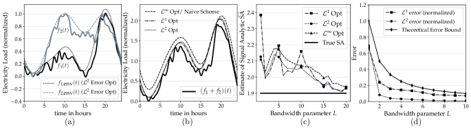
Figure 2: (a) Distributed envelope approximation applied on electricity load datasets collected from Eastern and Western Region power grids in India [17] for $L=3$ approximation coefficients (b) Sum envelope recovered at the IoT cloud using $\mathcal{L}^{q}\;\;q=1,2,\infty$ error optimization (c) Convergence of $\widehat{\mbox{SA}}$ to SA with increasing available bandwidth $L$ at IoT device (d) Error versus Bandwidth plots for $\mathcal{L}^{1}$ and $\mathcal{L}^{2}$ error metric compared to the theoretical upperbound with $C_{2}(q=1,2)=0.5$ (see Theorem IV.1).

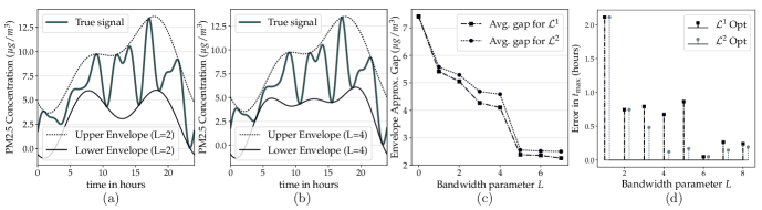
Figure 3: Dataset : PM2.5 (Speciation) concentration in Denver from US-EPA database [18](a) Lower and upper envelopes for $L=2$ with $\mathcal{L}^{2}$ optimization (b) Lower and upper envelopes for $L=4$ with $\mathcal{L}^{2}$ optimization (c) The variation of average gap between upper and lower envelopes with increasing values of $L$ (d) Error in time estimate of peak pollution concentration, $t_{\mbox{\scriptsize max}}$ for various value of $L$.

The main result is proved in this section.

Theorem IV.1

In (6) and (7), let $\mbox{SA}_{q}$ be the optimal distance and $\mbox{SA}^{\prime}_{q}$ be the distance corresponding to the naïve approximation in (9). There exist signals $f_{1}(t),\ldots,f_{M}(t)$ such that for $q=1,2,\infty$

$$C_{1}(q)\leq\frac{\mbox{SA}^{\prime}_{q}}{\mbox{SA}_{q}}\leq C_{2}(q)\mbox{ for }0<C_{1}(q)<C_{2}(q)<\infty.$$

Proof: Using (10) and the triangle inequality on sum of signals and their envelopes, we determine bounds on $\mbox{SA}_{q}$. They are tabulated in Table I, where the result follows for $q=2,\infty$ by taking ratios of $\mbox{SA}_{q}$ and $\mbox{SA}^{\prime}_{q}$. The steps are omitted due to space constraints. This result shows that the naive approximation is order optimal for the $\mathcal{L}^{2}$ and $\mathcal{L}^{\infty}$ errors, if the IoT device signals are $p$-times differentiable.

The optimality of the naïve envelopes for the $\mbox{SA}_{1}$ distance holds for a signal class with the following properties: (i) the Fourier coefficients $a_{1}[k]\geq 0$, and (ii) $f_{1}(t)$ is real and even, that is $a_{1}[k]=a_{1}[-k]$. ¿From these symmetry assumptions, it follows that $b_{1}[k]=b_{1}[-k]$. Restricted to this signal class, the $\mbox{SA}_{1}$ envelope approximation is re-stated as:

$$\operatorname*{arg\,min}_{b_{1}[k],|k|\leq L}b_{1}[0] ,\quad\text{subject to}$$

$$b_{1}[0]+2\sum_{1\leq|k|\leq L}b_{1}[k]\cos(2\pi kt) \geq\sum_{|k|>L}a_{1}[k]e^{j2\pi kt}$$ (11)

The above optimization can be shown to result in $b_{1,\text{\scriptsize opt}}[0]=\sum_{|k|>L}a_{1}[k]$ if $a_{1}[k]=0$ for $|k|<L$. In this case $a_{1}[0]=0$. And, for this signal $\mbox{SA}_{1}^{\prime}=C_{0}=\|f_{1}-f_{1,\mbox{\footnotesize proj}}\|_{\infty}\leq\sum_{|k|>L}a_{1}[k]$ as all the $a_{1}[k]$ Fourier coefficients are positive. Since $\mbox{SA}_{1}^{\prime}\geq\mbox{SA}_{1}$, as naive method will be suboptimal, so the two are equal.

It is noted that $\mbox{SA}_{1}$ and $\mbox{SA}^{\prime}_{1}$ in Table I are comparable. The presented result is for 1 IoT devices. For $M$ IoT devices, $\mbox{SA}_{1}$ and $\mbox{SA}_{\infty}$ as well as $\mbox{SA}^{\prime}_{1}$ and $\mbox{SA}^{\prime}_{\infty}$ scale linearly with $M$. And $\mbox{SA}_{2}$ as well as $\mbox{SA}^{\prime}_{2}$ scale quadratically with $M$. Their ratios remain the same as in $M=1$.

TABLE I: Bounds on the approximation errors

$\mathcal{L}^{q}$ error metric	$\mbox{SA}_{q}$	$\mbox{SA}^{\prime}_{q}$
$q=1$	$b_{1}[0]-a_{1}[0]$	$\begin{aligned} \sum_{|k|>L}|a_{1}[k]|\end{aligned}$
$q=2$	$\begin{aligned} \frac{2}{2p-1}\frac{1}{(L+1)^{2p-1}}\end{aligned}$	$\begin{aligned} \frac{2}{2p-1}\frac{1}{L^{2p-1}}\end{aligned}$
$q=\infty$	$\begin{aligned} \frac{2}{p-1}\frac{1}{(L+1)^{p-1}}\end{aligned}$	$\begin{aligned} \frac{2}{p-1}\frac{1}{L^{p-1}}\end{aligned}$

V Numerical simulations

Dataset Description: Time series data of electricity loads (in KWhr) from Eastern and Western region grids of India are considered [17] (see Fig. 2). The time samples available at 30 minute intervals are interpolated using low pass projection on Fourier basis with 25 coefficients. For brevity of simulations a normalized amplitude scale is used. We also consider the pollution dataset from US EPA [18], consisting of the time-series variation of PM2.5 concentration in Denver. The hourly sampled data, for a duration of 1 day, is smoothened using lowpass filtering using 10 Fourier coefficients (see Fig. 3).

Simulation setup and analysis: Simulations for the approximation error and bandwidth tradeoffs are presented for grid load data in Fig. 2 [17]. The time series plots for individual load variation are shown in Fig.2 (a). The sum signal envelope is reconstructed at the IoT Cloud with $(2L+1)=7$ Fourier coefficients (see Fig. 2(b)). The convergence of the estimate $\widehat{s}(t)$ to $s(t)$ with increasing $L$ is studied in Fig. 2(c). It is observed that the maxima of the sum signal is eventually tracked under each of the cost functions. The oscillations in the error plot (see Fig. 2 (c)) are the artifacts of the distributed and nonlinear nature of the approximation algorithm. At any IoT device, the maximum (nonlinear) of the signal is tracked with uniformly decreasing error. However, since each device independently (ie in a distributed manner) reports the approximations to the IoT cloud, the errors do not die down uniformly, but with occasional rise. Fig. 2(d) captures the bandwidth-error tradeoff for the three distance measures considered in the paper. The performance of the naïve approximation scheme is seen to coincide with that of the $\mathcal{L}^{\infty}$ error optimization. This is attributed to the relaxation of the $\mathcal{L}^{\infty}$ cost in terms of the coefficients as discussed in (5).

We analyze the gap between the upper and lower signal envelopes using the pollution dataset [18] (Fig. 3). We observe that the average gap between the envelopes decays with increasing value of $L$. It is to be noted that the lower envelope is negative in certain time intervals. In Fig. 3 (d) we analyze the error in time estimate of the peak pollutant concentration, $t_{\mbox{\scriptsize max}}$. The estimates approach the true value of signal analytic (ie $t_{\mbox{\scriptsize max}}$) eventually with growing bandwidth parameter $L$.

Energy consumption in IoT Device and IoT Cloud :By using IoT energy consumption data, a comparison of different IoT energy requirements are shown in Fig. 4 [19]. For a communication mode with $E_{b}$ energy/bit requirement and $B_{c}$ bits/coefficient, the proposed envelope scheme requires $(2L+1)E_{b}B_{c}$ energy units per device. The computing energy requirement (see Fig. 2(d)) is determined by counting the number of floating point operations (FLOP) in MATLAB to execute the optimization algorithm at the device. The conversion of FLOP to equivalent Joules is performed with respect to a 100 GFLOP/sec/W processor (see TI C667x processor [20]). It is observed that the communication and computation energy expenditure is observed to linear increase with the number of approximation coefficients.

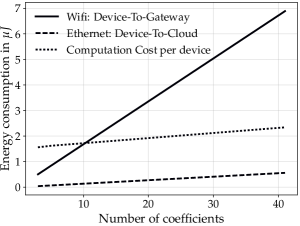
Figure 4: Energy expenditure at IoT device for communication and computing. Simulation parameters - $E_{b}=0.4279\;nJ/$bit for Ethernet, $5.25\;nJ/$bit for WiFi, bits per coefficient $B_{c}=32$ bits and $100$ GFLOPS/W processor.

VI Conclusions

Distributed nonlinear signal analytics was introduced for the first time. It was observed that in applications such as energy distribution, signal observed by IoT devices should be subjected to envelope approximation. An algorithm for over-predictive nonlinear signal analytics in the IoT cloud was developed in this work, by using the envelope approximation technique. The fundamental tradeoff between approximation error in signal analytics ($\mbox{SA}_{q},q=1,2,\infty$) and the bandwidth parameter $L$ was established. It was observed that this tradeoff depends on the smoothness of signals at the IoT devices. Simulation results were presented for load data collected from two power grids. Envelope approximation schemes using polynomial and wavelet basis are proposed as a future extensions.

References

- [1] T.M. Cover and J.A. Thomas, Elements of Information Theory, John Wiley and Sons, 2006.
- [2] C. E. Shannon, “Communication in the presence of noise,” Proceedings of the IRE, vol. 37, no. 1, pp. 10–21, Jan 1949.
- [3] Ronald A. DeVore and George G. Lorentz, Constructive Approximation, Springer, 1993.
- [4] A. Zanella, N. Bui, A. Castellani, L. Vangelista, and M. Zorzi, “Internet of things for smart cities,” IEEE Internet of Things Journal, vol. 1, no. 1, pp. 22–32, Feb 2014.
- [5] A. Giridhar and P. R. Kumar, “Computing and communicating functions over sensor networks,” IEEE Journal on Selected Areas in Communications, vol. 23, no. 4, pp. 755–764, April 2005.
- [6] P. Vyavahare, N. Limaye, and D. Manjunath, “Optimal embedding of functions for in-network computation: Complexity analysis and algorithms,” IEEE/ACM Transactions on Networking, vol. 24, no. 4, pp. 2019–2032, Aug 2016.
- [7] P. Jesus, C. Baquero, and P. S. Almeida, “A survey of distributed data aggregation algorithms,” IEEE Communications Surveys Tutorials, vol. 17, no. 1, pp. 381–404, Firstquarter 2015.
- [8] J. Ranieri, I. Dokmanic, A. Chebira, and M. Vetterli, “Sampling and reconstruction of time-varying atmospheric emissions,” in 2012 IEEE International Conference on Acoustics, Speech and Signal Processing (ICASSP), March 2012, pp. 3673–3676.
- [9] Animesh Kumar, “Optimal envelope approximation in fourier basis with applications in TV white space,” arXiv, 2017, Available at http://arxiv.org/abs/1706.00900.
- [10] John Nikolas Tsitsiklis, Problems in Decentralized Decision Making and Computation, Ph.D. thesis, Massachusetts Institute of Technology. Laboratory for Information and Decision Systems, 1984.
- [11] Y. Sun, H. Song, A. J. Jara, and R. Bie, “Internet of things and big data analytics for smart and connected communities,” IEEE Access, vol. 4, pp. 766–773, 2016.
- [12] J. Jin, J. Gubbi, S. Marusic, and M. Palaniswami, “An information framework for creating a smart city through internet of things,” IEEE Internet of Things Journal, vol. 1, no. 2, pp. 112–121, April 2014.
- [13] Alan V Oppenheim, Discrete-time signal processing, Pearson Education India, 1999.
- [14] Stephane Mallat, A Wavelet Tour of Signal Processing, Third Edition: The Sparse Way, Academic Press, 3rd edition, 2008.
- [15] G. Maheshwari and A. Kumar, “Optimal quantization of tv white space regions for a broadcast based geolocation database,” in 2016 24th European Signal Processing Conference (EUSIPCO), Aug 2016, pp. 418–422.
- [16] Rajendra Bhatia, Fourier Series, Hindustan Book Agency, 2nd edition, 1993.
- [17] Power System Operation Corporation Ltd., “Electricity load factor in Indian power system,” Report of the National Load Dispatch Center, 2016.
- [18] “Tables of hourly data for particulates,” https://www.epa.gov/outdoor-air-quality-data, Accessed: 2018-02-20.
- [19] Internet Society, “The Internet of Things (IoT): An Overview,” 2015.
- [20] “TMS320C6678 multicore fixed and floating-point digital signal processor,” http://www.ti.com/lit/ds/symlink/tms320c6678.pdf, Accessed: 2018-02-20.