Non-parametric Structural Change Detection in Multivariate Systems

Abstract

Structural change detection problems are often encountered in analytics and econometrics, where the performance of a model can be significantly affected by unforeseen changes in the underlying relationships. Although these problems have a comparatively long history in statistics, the number of studies done in the context of multivariate data under nonparametric settings is still small. In this paper, we propose a consistent method for detecting multiple structural changes in a system of related regressions over a large dimensional variable space. In most applications, practitioners also do not have a priori information on the relevance of different variables, and therefore, both locations of structural changes as well as the corresponding sparse regression coefficients need to be estimated simultaneously. The method combines nonparametric energy distance minimization principle with penalized regression techniques. After showing asymptotic consistency of the model, we compare the proposed approach with competing methods in a simulation study. As an example of a large scale application, we consider structural change point detection in the context of news analytics during the recent financial crisis period.

1 Introduction

Interest towards large dimensional multivariate regression and interdependence analysis has surged due to their relevance for mining predictive relationships out of massive data sets (Yuan et al., 2007; Negahban and Wainwright, 2011). Many of these problems are characterized by the dual challenge of learning several related models simultaneously while allowing them to account for a large pool of candidate variables that are partly shared across the individual relationships (Abernethy et al., 2009; Negahban and Wainwright, 2011; Agarwal et al., 2012). Such large dimensional modeling tasks are commonly encountered in practical applications, such as financial forecasting, news analytics, or marketing, where the objective is to predict the development of many possibly related indicators simultaneously (Stock and Watson, 2009; Groen et al., 2013; Fan et al., 2011). However, a further layer of complexity is introduced, when the underlying predictive relationships are recognized to undergo multiple structural changes when longer time periods are considered (Qian and Su, 2016; Chopin, 2006; Bai and Perron, 1998, 2003). For example, in marketing applications, it is rational to expect that consumer preferences can change rapidly in response to major product or technological innovations. Often, the practitioner also does not have a priori information on the relevance of the candidate variables, and therefore it becomes natural to let the data decide which variables should be retained. When combined with the requirement of detecting an unknown number of change points in multivariate data, encountering the simultaneous variable selection problem limits the applicability of earlier methods, which assume either a fixed and typically very small set of contributing explanatory variables (Li and Perron, 2017; Qu and Perron, 2007) or investigate only single equation models (Bai and Perron, 2003).

In this paper, we consider large dimensional regression problems, where the objective is to estimate a collection of related regressions over a varying set of features while allowing the model to be exposed to multiple structural changes. A structural change is defined as a point that separates a time-ordered sample into two parts having different linear structures. Throughout, we treat both number as well as locations of the structural change points as unknown variables. We also assume that the model structure is sparse and that the potential structural changes take place in a discontinuous manner, where both parameter estimates as well as the number of variables with non-zero coefficients can vary from one regime to another. Further, we do not make any assumptions regarding the underlying distribution beyond the requirement of very weak moment conditions on the regressors and residuals. Since this kind of problem is typically ill-posed due to the dimensionality concerns, it is natural to impose sparsity constraints or regularization on the problem. Regularization is formulated as a convex optimization problem consisting of a loss term and a regularizer. The framework of this paper works under very general requirements for the admissible regularizers as well as loss functions.

Our paper has two main objectives. The first is to propose a non-parametric method that can consistently estimate an unknown number of structural change points in a large dimensional multivariate linear regression model. To avoid imposing distributional assumptions, we approach the problem using an energy distance framework that is based on $U$-statistics (Rizzo and Székely, 2016; Székely and Rizzo, 2014a, b, 2005). The asymptotic results are obtained under quite general conditions. The second objective is to look at the problem from algorithm-design perspective, and ensure that the estimation principle can be implemented in a computationally efficient manner. To address this, two algorithms are suggested. The first is based on the principle of dynamic programming, which has been successfully applied also in the earlier literature by Bai and Perron (2003). This approach gives a consistent way to obtain the global minimizers of energy distance statistic. However, it remains computationally quite demanding, and requires $O(T^{2})$ operations for any given number of structural change points. The second algorithm is a more efficient heuristic with performance of order $O(T)$ but with no guarantee of finding the global minimizers. However, our extensive simulation study gives evidence on its ability to detect the structural changes with an accuracy that is on par with the dynamic programming principle. Therefore, it can be a preferred choice for practitioners dealing with large models and long time periods that usually have many structural changes. As an example, we consider structural change detection in the context of news analytics.

Though change point analysis has attracted widespread attention across different fields (Cho and Fryzlewicz, 2015), the literature on structural change detection, especially in the context of systems of multivariate equations, has remained relatively sparse (Li and Perron, 2017; Qu and Perron, 2007; Kurozumi and Arai, 2007). Whereas change point analysis commonly refers to detection of breaks in trend or distributional changes (e.g., shift in mean or variance) in univariate or multivariate series  (Ruggieri and Antonellis, 2016; Matteson and James, 2014; Harchaoui and Lévy-Leduc, 2010), structural change analysis is focused on detecting changes in the underlying predictive relationship (Bai and Perron, 2003; Qu and Perron, 2007; Qian and Su, 2016; Li and Perron, 2017). Hence, along with changes in distribution or trend, breaks can be attributed to shifts in the model parameters or changes in the pool of relevant explanatory variables. Although, the two lines of research, change point analysis and structural change analysis, have evolved simultaneously, their development has been driven by different fields of study. While change point analysis (or data segmentation (Fryzlewicz, 2014)), has been directly motivated by applications in signal processing and bioinformatics, structural change analysis is popular in social disciplines, business and economics (Bai and Perron, 2003; Qu and Perron, 2007; Qian and Su, 2016).

Another important distinction in literature is made between parametric and nonparametric setups. In parametric change point analysis, the underlying distributions are assumed to belong to some known family that admits use of log-likelihood functions in the analysis (Davis et al., 2006; Lebarbier, 2005; Lavielle and Teyssière, 2006). Recently, non-parametric methods have gained traction as they are considered applicable to a wider range of applications (Matteson and James, 2014; Hariz et al., 2007). However, many of these approaches require estimation of density functions or density ratios (Kawahara and Sugiyama, 2012; Kanamori et al., 2009; Liu et al., 2013). Also rank statistics and energy distance statistics have been considered (Matteson and James, 2014). One of the key benefits of energy statistics is their simplicity. Since they are based on Euclidean distances (Székely and Rizzo, 2005), the energy statistics are easy to compute also in multivariate settings. However, it is noted that these nonparametric approaches have been proposed in the context of change point analysis to detect distributional changes rather than structural breaks. In this paper, we show how the idea of using energy distance statistics for distributional change detection (Matteson and James, 2014) can be extended to structural change detection in models with large number of potential explanatory variables.

Against this backdrop, we propose a new nonparametric method for detecting structural changes in multivariate data. In comparison to the literature, our work differs in three aspects. First, we allow the modeling to take place with large pool of candidate variables, and acknowledge that each structural change can be accompanied by change in the collection of variables with non-zero coefficients, which is quite different from the settings in Bai and Perron (2003); Qu and Perron (2007) and Li and Perron (2017). Also, unlike Qian and Su (2016) who employ group fused lasso penalty to detect change point locations, we use sparsity constraints to guide variable selection within regimes rather than to detect the regime boundaries. Based on the experiments, our approach appears to produce more parsimonious models in terms of the number of change points. Second, the use of nonparametric energy statistics allows us to relax important distributional assumptions. In particular, this has the benefit of reducing sensitivity towards outliers and fat-tailed residual distributions. Finally, differing from most of the prior work, our method is designed to handle change point detection in multivariate systems of equations rather than restricting to a single predictive relationship (Qian and Su, 2016; Bai and Perron, 2003).

The rest of the paper is organized as follows. In Section 2, we present the model and the estimation principle based on minimization of energy distances. Section 3 discusses definitions and properties of energy distance statistics. Section 4 presents assumptions and the asymptotic consistency results for the model. This is followed by description of nonparametric goodness-of-fit statistics in Section 5, which are then used to guide the algorithms are outlined in Section 6. In Section 7, we show the results from computational studies, where our approach applied to simulated and real data. As an example of a large scale problem, we consider structural change detection in the context of business news analytics, where the objective is to understand how different types of financial news events are reflected company valuations. Concluding remarks are given in Section 8.

2 Model

Consider the following multiple regression model with $k$ change points ($k+1$ regimes):

$$y_{t}=x_{t}^{\prime}\beta_{j}+u_{t},\quad t=T_{j-1}+1,\dots,T_{j}$$

for $j=1,\dots,k+1$. By convention we have that $T_{0}=0$ and $T_{k+1}=T$. In this model, $y_{t}\in\mathbb{R}^{q}$ denotes an observed independent variable, $u_{t}\in\mathbb{R}^{q}$ is the disturbance, $x_{t}\in\mathbb{R}^{p}$ is a vector of covariates, and $\beta_{j}\in{\mathbb{R}}^{p\times q}$ $(j=1,\dots,k+1)$ are the corresponding matrix of coefficients. Throughout the paper we denote by $|\cdot|$ the Euclidean norm and by $\|\cdot\|$ the corresponding operator norm for the matrices. Note that the norms depend on the dimensions which we have omitted on the notation. The sequence of unknown break points are denoted by indices $(T_{1},\dots,T_{k})$. The purpose is to estimate the unknown regression coefficients and the change points based on the observed data $(y_{t},x_{t})$. Throughout the paper, we denote the true value of a parameter with a 0 superscript. In particular, the true values for coefficients and the change points are denoted by $\beta^{0}=(\beta_{1}^{0},\dots,\beta_{k+1}^{0})$ and $(T_{1}^{0},\dots,T_{k}^{0})$, respectively. In general, the number of change points can be assumed to be an unknown variable with true value of $k^{0}$. However, to simplify our discussion on the general estimation principles, we will for now treat the number of change points $k$ as known. Methods for estimating $k$ will be presented in later parts of the paper.

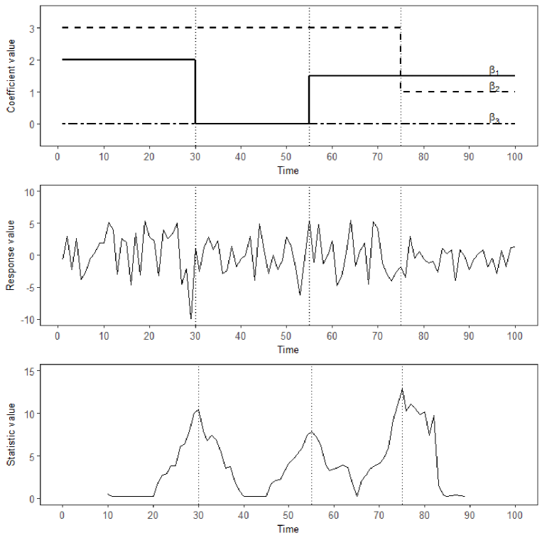
Figure 1: Energy-distance based detection of structural changes in a single equation model with 4 regimes and 3 variables. Locations of the structural changes are highlighted by dashed vertical lines. The first graph shows the evolution of coefficients over time and second graph shows the time series for the response variable. The third graph shows the corresponding changes in the energy-distance measure, which is used to detect the regime boundaries.

The estimation method is constructed as a hybrid of penalized regression technique and non-parametric testing strategy. We assume that the coefficients $\{\beta_{j}\}$ representing different regimes exhibit sparsity such that the effective number of non-zero coefficients in each $\beta_{j}$ is less than $p$. The large number of potential covariates motivates the use of regularization techniques. Given a $k$-partitioning $\{T_{j}\}=(T_{1},\dots,T_{k})$, the estimates of $\beta$ are obtained as minimizers of the empirical risk

$$(\hat{\beta}_{1},\dots,\hat{\beta}_{k+1})=\mathop{\rm argmin}\limits_{\beta}\mathcal{L}_{T}(\beta;\{T_{j}\})=\sum_{j=1}^{k+1}\sum_{t=T_{i-1}+1}^{T_{i}}\psi(x_{t}^{\prime}\beta_{j}-y_{t})+\gamma_{n}\varphi(\beta),$$ (1)

where $\psi$ is a strictly convex loss function and $\varphi$ is a convex function such that both $\psi$ and $\varphi$ attain their global minimums at zero. To highlight the dependence on the partitioning, the penalized estimates are denoted by $\hat{\beta}(\{T_{j}\})$. Substituting these into the model equation gives us estimates of the regression residuals. Let $\mathcal{U}=\{U_{1},\dots,U_{k+1}\}$ represent the partitioning of the regression residuals $\hat{u}_{t}$ into clusters such that $U_{j}=\{\hat{u}_{T_{j-1}+1},\dots,\hat{u}_{T_{j}}\}$. The change points are then defined as global minimizers of the goodness-of-fit statistic

$$(\hat{T}_{1},\dots,\hat{T}_{k})=\mathop{\rm argmin}\limits_{T_{1},\dots,T_{k}}\sum_{1\leq i<j\leq k+1}\left(\frac{n_{i}+n_{j}}{2T}\right)d_{\alpha}(U_{i},U_{j}),$$ (2)

where $n_{i}$ and $n_{j}$ denote the sample sizes of $U_{i}$ and $U_{j}$, respectively. The minimization is taken over all partitions of the timeline such that $T_{j}-T_{j-1}\geq\varepsilon T$ for some $\varepsilon>0$. The function $d_{\alpha}$ is a measure of the empirical distance between the distributions of the partitioned disturbances by Székely and Rizzo (2014a, b, 2005). Here the objective is to detect the change points such that the partitioned model residuals $\mathcal{U}$ can be interpreted as $k+1$ random samples from distributions with cumulative distribution function $F_{1},\dots,F_{k+1}$, for which the null hypothesis of equal distributions $H_{0}:F_{1}=\cdots=F_{k+1}$ holds. The test is implemented as a bootstrap statistic, which is discussed in Section 5.

A stylized example of the approach is given in Figure 1, which shows functioning of the model in a single equation example with only three variables and four regimes, i.e. $q=1$, $p=3$ and $k=3$. The number of non-zero variables can change in any regime and not all candidate variables need to contribute to the relation. In this example, the model residuals and explanatory variables are all normally distributed. However, as shown by our experiments, the relative benefits of our model are mainly realized in large dimensional settings, where the normality assumption is not met due to presence of outliers or fat-tailed residuals. These are the circumstances, where the use of non-parametric energy-distance becomes helpful. To further motivate our approach, we will in next section discuss the key properties of $d_{\alpha}$ and introduce the notion of energy distance as a non-parametric measure of dispersion that can be computed based on Euclidean distances between all pairs of sample elements.

Remark 1.

Occurrence of a structural change does not necessarily imply a distributional change in the joint distribution of $(y_{t},x_{t})$. A simple example could be constructed using a model with only two explanatory variables and a single response, where the explanatory variables follow the same distribution. Then a time point, where the coefficients of the two explanatory variables get exchanged, would not count as a distributional change point, but would still be considered a structural change point that should be detected.

3 Energy distance

Energy distance is a metric that measures the distance between the distributions of random vectors, which was introduced and popularized by Rizzo and Székely (2016); Székely and Rizzo (2014a, b, 2005). The energy distance is zero if an only if the distributions are identical, otherwise it will diverge. The notion derives from the concept of Newton’s potential energy by considering statistical observations as objects in a metric space that are governed by statistical potential energy. Since its introduction the energy distance and the more general class of energy statistics have been utilized in a number of applications ranging from testing independence by distance covariance to non-parametric tests for equality of distributions. Our study as well as the e-divisive algorithm by Matteson and James (2014) show how energy distance can be utilized for analysis of change points or structural breaks in time series data.

3.1 Energy distance for two samples

As proven by Székely and Rizzo, it can be shown that energy distance satisfies all axioms of a metric, and therefore it provides a characterization of equality of distributions as well as a theoretical basis for development of multivariate analysis based on Euclidean distances.

Lemma 1.

Suppose $u,u^{\prime}\stackrel{{\scriptstyle iid}}{{\sim}}F_{u}$ and $v,v^{\prime}\stackrel{{\scriptstyle iid}}{{\sim}}F_{v}$, and that $u,u^{\prime},v$, and $v^{\prime}$ are mutually independent random variables in $\mathbb{R}^{d}$. If $E(|u|^{\alpha}+|v|^{\alpha})<\infty$, for any $\alpha\in(0,2)$, then the characteristic function based divergence measure between distributions can be defined based on Euclidean distances as

$$\mathcal{E}(u,v;\alpha)=2E|u-v|^{\alpha}-E|u-u^{\prime}|^{\alpha}-E|v-v^{\prime}|^{\alpha}$$

such that $\mathcal{E}(u,v;\alpha)=0$ if and only if $u$ and $v$ are identically distributed.

The corresponding empirical divergence measure can then be defined in the spirit of $U$-statistics. If $V_{n}=\{v_{i}:i=1,\dots,n\}$ and $W_{m}=\{w_{j}:j=1,\dots,m\}$ are independent iid samples from distributions $F_{v}$ and $F_{w}$, such that $E|v|^{\alpha},E|w|^{\alpha}<\infty$, we can use the divergence to define the empirical energy distance measure as

$$\begin{split}d_{\alpha}(V_{n},W_{m})&=\frac{mn}{m+n}\hat{\mathcal{E}}(V_{n},W_{m};\alpha)\\ &=\frac{mn}{m+n}(2\hat{\mu}^{\alpha}_{vw}-\hat{\mu}^{\alpha}_{v}-\hat{\mu}^{\alpha}_{w}),\end{split}$$ (3)

where

$$\hat{\mu}^{\alpha}_{vw}=\frac{1}{mn}\sum_{i=1}^{n}\sum_{j=1}^{m}|v_{i}-w_{j}|^{\alpha},\quad\hat{\mu}^{\alpha}_{v}=\binom{n}{2}^{-1}\sum_{1\leq i<k\leq n}|v_{i}-v_{k}|^{\alpha},\quad\text{and}$$

$$\hat{\mu}^{\alpha}_{w}=\binom{m}{2}^{-1}\sum_{1\leq j<k\leq m}|w_{j}-w_{k}|^{\alpha}.$$

This empirical measure is based on Euclidean distances between sample elements and is $O(\max{(m^{2},n^{2})})$. Under the given assumptions, the strong law of large numbers for U-statistics Hoeffding (1961) and continuity theorem imply that $\hat{\mathcal{E}}(V_{n},W_{m};\alpha)\to\mathcal{E}(v,w;\alpha)$ almost surely as $n,m\to\infty$. When equal distributions are assumed, the energy distance measure $d_{\alpha}(V_{n},W_{n})$ convergences to a non-degenerate random variable. Conversely, if the distributions are unequal, it follows that the energy distance diverges, i.e. $d_{\alpha}(V_{n},W_{m})\to\infty$ almost surely as $n,m\to\infty$, since $\mathcal{E}(v,w;\alpha)>0$ for unequal distributions.

3.2 Multi-sample energy distance

For any partitioning $\{T_{j}\}$, let $S_{\alpha}$ denote the objective function in (2), i.e.

$$S_{\alpha}(U_{1},\dots,U_{k+1})=\sum_{1\leq i<j\leq k+1}\left(\frac{n_{i}+n_{j}}{2T}\right)d_{\alpha}(U_{i},U_{j})$$ (4)

where $U_{j}=\{\hat{u}_{T_{j-1}+1},\dots,\hat{u}_{T_{j}}\}$ is the sequence of residuals from regime $j$. As seen from the following corollary of Lemma 1, $S_{\alpha}$ statistic can be viewed as a multi-sample extension of the two-sample distance measure introduced in Section 3.1.

Corollary 1.

For all $p$-dimensional samples $U_{1},\dots,U_{k+1}$, $k\geq 1$, and $\alpha\in(0,2)$, the following statements hold: (i) $S_{\alpha}(U_{1},\dots,U_{k+1})\geq 0$; and (ii) $S_{\alpha}(U_{1},\dots,U_{k+1})=0$ if and only if $U_{1},\dots,U_{k+1}$ are equally distributed.

The proof of the result is obtained by applying induction argument on Lemma 1. It is clear from the construction that the statistic is likely to share many interesting similarities with ANOVA. By interpreting $S_{\alpha}$ as a multi-sample test of equal distributions, it can be considered as a type of generalization of the hypothesis of equal means. In fact, as shown by Rizzo and Székely (2010), the connection to analysis of variance can be obtained through the special case $\alpha=2$, when the $d_{2}$-distance for a univariate response variable measures variance.

4 Consistency

In this section, we study the consistency of the estimated change point fractions in the case of a single change point as well as the generalization of the result into the case of multiple change points. We denote the estimated change point fractions and their corresponding true values by $\hat{\lambda}=(\hat{\lambda}_{1},\dots,\hat{\lambda}_{k})=(\hat{T}_{1}/T,\dots,\hat{T}_{k}/T)$ and $\lambda^{0}=(\lambda_{1}^{0},\dots,\lambda_{k}^{0})$, respectively.

Throughout the following discussions on the statistical properties of the estimators, we will rely on the following assumptions.

Assumption $\mathbf{A}$1.

The change points are asymptotically distinct such that $T_{i}^{0}=[T\lambda_{i}^{0}]$, where $0<\lambda_{1}^{0}<\cdots<\lambda_{k}^{0}<1$ and $\lambda_{0}^{0}=0$ and $\lambda_{k+1}^{0}=1$.

Assumption $\mathbf{A}$2.

The model regressors $x_{t}$ are identically distributed within regions, i.e. $x_{t}\sim X_{k}$ for every $T_{k-1}+1\leq t\leq T_{k}$. Furthermore we have, for a given $\alpha\in(0,2)$, that $E(|x_{t}|^{2\alpha})<\infty$.

Assumption $\mathbf{A}$3.

The model disturbances $u_{t}$ are independent and identically distributed. Further, the disturbances $u_{t}$ are assumed to be independent of the regressors $x_{s}$ for all $t$ and $s$. Finally, we assume that, for a given $\alpha\in(0,2)$, we have $E(|u_{t}|^{2\alpha})<\infty$.

Assumption $\mathbf{A}$4.

For any given change points $T_{i},i=1,2,\ldots,k$, the regularized estimators $\hat{\beta}_{i}$ converges in probability to some constant $\beta^{c}_{i}$. That is, we have $\|\hat{\beta}_{i}-\beta^{c}_{i}\|\rightarrow 0$ in probability. Moreover, for any $i$, the regularized estimator $\hat{\beta}_{i}$ is consistent only if $T_{i}^{0}\leq T_{i}<T_{i+1}\leq T_{i+1}^{0}$.

Assumption $\mathbf{A}$5.

Let $c_{1},c_{2}\in{\mathbb{R}}^{p\times q}$ be arbitrary matrices and let

$$Y_{i,j}=|u_{i}-u_{j}+x_{i}^{\prime}c_{1}-x_{j}^{\prime}c_{2}|^{\alpha},$$

where $T_{k-1}+1\leq i,j\leq T_{k}$ for some $k$. We assume that the regressors $x_{s}$ are asymptotically independent in the sense that, as

$$\min_{l,j\in\{1,2,3,4\},l\neq j}|i_{l}-i_{j}|\rightarrow\infty,$$

we have

$$Cov(Y_{i_{1},i_{2}},Y_{i_{3},i_{4}})\rightarrow 0$$

and

$${\mathbb{E}}[Y_{i_{1},i_{2}}]\rightarrow{\mathbb{E}}|U-\tilde{U}+X_{k}^{\prime}c_{1}-\tilde{X}_{k}^{\prime}c_{2}|^{\alpha},$$

where $U,\tilde{U}$ are independent copies of $u$ and $X^{\prime},\tilde{X}^{\prime}$ are independent copies of $x$.

The first technical assumption is very natural. Indeed, if the change points are not (asymptotically) distinct, then one may simply remove one. The second and the third technical assumptions give moment conditions and distributional assumptions for the regressors and for the disturbance terms that guarantee the convergence of the empirical energy distances.

The fourth technical assumption is also a natural one. The first statement of the assumption means that, as the number of observations increase, the regularized estimators converge to some constants. We emphasize the fact that the constants might be, and usually are, wrong ones, unless the change points are estimated correctly. Moreover, the consistency assumption states that the regularized estimators are consistent if the estimation is based on the observations lying on the correct intervals.

The fifth technical assumption is used to guarantee the convergence of the empirical energy distances to some constant quantities. This assumption simply states that the regressors are asymptotically independent. (Assumption that is widely used in the literature). The intuition behind this assumption is that, as the number of observations increase on every subinterval, one can think that the dependence of the regressors between fixed time points is spread among the time points in the middle.

Note that these assumptions are quite mild. Typical vector autoregressive models, for example, fulfill the above assumptions A1-A5.

4.1 Single change point

In order to obtain consistency, we apply the following elementary lemma providing a version of weak law of large numbers for weakly dependent double arrays.

Lemma 2.

Let $X_{i_{1},i_{2}},i_{1},i_{2}=1,\ldots,n$ denote a double array of random variables with

$$\sup_{i_{1},i_{2}}{\mathbb{E}}(X^{2}_{i_{1},i_{2}})<\infty.$$

Assume there exists a constant $C\in{\mathbb{R}}$ such that

$${\mathbb{E}}\left[(X_{i_{1},i_{2}}-C)(X_{i_{3},i_{4}}-C)\right]\rightarrow 0$$

as $\min_{k,j\in\{1,2,3,4\},k\neq j}|i_{k}-i_{j}|\rightarrow\infty.$ Then, as $n\rightarrow\infty$, $\frac{1}{n^{2}}\sum_{i_{1},i_{2}=1}^{n}X_{i_{1},i_{2}}\rightarrow C$ in probability.

The proof of Lemma 2 is provided in Appendix A.1. Now together with assumptions A1-A5, we can show the consistency of the estimator in the case of a single change point.

Proposition 1.

Let $\hat{T}_{1}$ denote the estimated energy-distance minimizing change point location, as defined in equation (2). Suppose that $\frac{\hat{T}_{1}}{T}$, as $T\to\infty$, converges in probability to $\hat{\lambda}_{1}\in(0,1)$. Then, under A1-A5, we have $\hat{\lambda}_{1}=\lambda_{1}^{0}$.

The proof is obtained by contradiction (see Appendix A.2 for detailed proof). Assume that $\lambda_{1}^{0}$ is not consistently estimated, i.e. $\hat{\lambda}_{1}\neq\lambda_{1}^{0}$. Without loss of generality, we assume that the estimated change point $\hat{T}_{1}$ satisfies $\hat{T}_{1}<T\lambda_{1}^{0}$, giving us a partitioning $I_{1}=[0,\hat{T}_{1}]$, $I_{2}=[\hat{T}_{1}+1,T_{1}^{0}]$ and $I_{3}=[T_{1}^{0}+1,T]$.

We denote by $|A|$ the size of a set $A$. In particular, we have that $|I_{1}\cup I_{2}\cup I_{3}|=T$, $|I_{3}|=(1-\lambda_{1}^{0})T$, $|I_{1}|\sim\hat{\lambda}_{1}T$, $|I_{2}|\sim(\lambda_{1}^{0}-\hat{\lambda}_{1})T$, and $|I_{2}\cup I_{3}|\sim(1-\hat{\lambda}_{1})T$ (where the notation $f(T)\sim g(T)$ refers to the usual interpretation $\lim_{T\to\infty}\frac{f(T)}{g(T)}=1$). For notational simplicity, we denote by $\hat{\beta}(i)$ the estimator corresponding to the region where $i$ belongs. That is, for $\hat{\beta}_{i},i=1,2$ denoting the regularized estimates, we have $\hat{\beta}(i)=\hat{\beta}_{1}$ for all $i\in I_{1}$, and $\hat{\beta}(i)=\hat{\beta}_{2}$ for all $i\in I_{2}\cup I_{3}$. Similarly, we denote by $\beta^{0}(i)$ the correct value corresponding to the region where $i$ belongs. That is, as the true change point is $T_{1}^{0}$, we have $\beta^{0}(i)=\beta^{0}_{1}$ for all $i\in I_{1}\cup I_{2}$ and $\beta^{0}(i)=\beta^{0}_{2}$ for all $i\in I_{3}$. We also denote by $\beta(i)$ and $\beta^{c}_{k}$ the limits related to Assumption 4. More precisely, we always have $\hat{\beta}(i)\rightarrow\beta(i)$ and $\hat{\beta}_{k}\rightarrow\beta^{c}_{k}$. Moreover, we have $\hat{\beta}(i)=\hat{\beta}_{1}\rightarrow\beta^{c}_{1}=\beta^{0}_{1}$ for all $i\in I_{1}$, as region $I_{1}$ is a subset of the correct interval $[0,T_{1}^{0}]$. For $i\in I_{2}\cup I_{3}$, we have $\hat{\beta}(i)=\hat{\beta}_{2}\rightarrow\beta^{c}_{2}$, and thus $\beta(i)=\beta^{c}_{2}$.

Denote by $\hat{u}_{i}=u_{i}-x_{i}^{\prime}(\hat{\beta}(i)-\beta^{0}(i)),i\in I_{k},k=1,2,3$ the corresponding estimated residuals and let $U_{1}=\{\hat{u}_{t}\}_{t\in I_{1}}$ and $U_{2}=\{\hat{u}_{t}\}_{t\in I_{2}\cup I_{3}}$ denote the collections of regularized residuals from different intervals. We set

$$\hat{\mu}^{\alpha}_{U_{1},U_{2}}=\frac{1}{|I_{1}||I_{2}\cup I_{3}|}\sum_{j\in I_{1},i\in I_{2}\cup I_{3}}|\hat{u}_{i}-\hat{u}_{j}|^{\alpha},\hat{\mu}^{\alpha}_{U_{1}}=\frac{1}{|I_{1}|^{2}}\sum_{i,j\in I_{1}}|\hat{u}_{i}-\hat{u}_{j}|^{\alpha},$$

and

$$\hat{\mu}^{\alpha}_{U_{2}}=\frac{1}{|I_{2}\cup I_{3}|^{2}}\sum_{i,j\in I_{2}\cup I_{3}}|\hat{u}_{i}-\hat{u}_{j}|^{\alpha}.$$

We prove that

$$2\hat{\mu}^{\alpha}_{U_{1},U_{2}}-\hat{\mu}^{\alpha}_{U_{1}}-\hat{\mu}^{\alpha}_{U_{2}}\rightarrow C>0,$$ (5)

where $C$ is a constant and the convergence holds in probability. From this we get

$$d_{\alpha}(U_{1},U_{2})=\frac{|I_{1}||I_{2}\cup I_{3}|}{2|I_{1}|+2|I_{2}\cup I_{3}|}\left(2\hat{\mu}^{\alpha}_{U_{1},U_{2}}-\hat{\mu}^{\alpha}_{U_{1}}-\hat{\mu}^{\alpha}_{U_{2}}\right)\rightarrow\infty.$$

Consequently, $\hat{T}_{1}$ cannot be a minimizer for the model equation 2 of Section 2 (in the paper), which leads to the expected contradiction.

We divide the rest of the proof into three steps. In step 1 we consider the differences $\hat{u}_{i}-\hat{u}_{j}$ that depend on the entire data set. In step 2 we calculate the limits of the terms $\hat{\mu}^{\alpha}_{U_{1},U_{2}}$, $\hat{\mu}^{\alpha}_{U_{1}}$, and $\hat{\mu}^{\alpha}_{U_{2}}$. Finally, in step 3, we show (18). For complete technical proof, see Appendix A.2.

4.2 Multiple change points

Having established consistency in the case of a single change point, it is now straightforward to extend the result to the case of multiple change points.

Proposition 2.

Let $\hat{T}_{j},j=1,\ldots,k$ denote the estimated energy-distance minimizing change point locations, as defined in equation (2). Suppose that, for all $j=1,\ldots,k$, as $T\to\infty$, the quantity $\frac{\hat{T}_{j}}{T}$ converges in probability to $\hat{\lambda}_{j}\in(0,1)$. Then, under A1-A5, $\hat{\lambda}_{j}=\lambda_{j}^{0}$ for all $j=1,\ldots,k$.

The proof is again obtained by assuming contradiction and using Proposition 1 together with Lemma 2. The technical details of the proof are provided in Appendix A.3.

5 Non-parametric change point tests

The estimates from (1) and (2) are consistent when the number of actual change points is known. However, in practice, the number of true change point is generally not known. Therefore, in order to construct a suitable algorithm, we need a test statistic that allows us to check whether the proposed partitioning produces an acceptable fit.

5.1 Goodness of fit test for $k$ change point model

Let $(T_{1},\dots,T_{k})$ be any hypothesized sequence of change points, and let $(U_{1},\dots,U_{k+1})$, $U_{i}\sim F_{i}$, denote the corresponding sequences of model residuals for the $k+1$ regimes. To test for homogeneity in distribution,

$$H_{0}:F_{1}=\cdots=F_{k+1},k\geq 1,$$ (6)

versus the composite alternative $F_{i}\neq F_{j}$ for some $1\leq i<j\leq k+1$, we can apply the distance components statistic by Rizzo and Székely (2010). If $H_{0}$ is rejected, we conclude that there is at least one change point that has not been identified.

The test statistic is constructed in a manner analogous to ANOVA, and it is based on the following decomposition theorem that is obtained by direct application of the results in Rizzo and Székely (2010) on the $k$ change point problem. Define the total dispersion of the estimated regime residuals as

$$T_{\alpha}(U_{1},\dots,U_{k+1})=\frac{T}{2}\mu_{\alpha}(U,U),$$ (7)

where $U=\sum_{j=1}^{k+1}U_{j}$ is the pooled sample of regime residuals, and

$$\mu_{\alpha}(A,B)=\frac{1}{n_{1}n_{2}}\sum_{i=1}^{n_{1}}\sum_{j=1}^{n_{2}}|a_{i}-b_{j}|^{\alpha}$$

for any sets $A$ and $B$ of size $n_{1}$ and $n_{2}$, respectively. Similarly, we can define the within-sample dispersion statistic as

$$W_{\alpha}(U_{1},\dots,U_{k+1})=\sum_{j=1}^{k+1}\frac{n_{j}}{2}\mu_{\alpha}(U_{j},U_{j})$$ (8)

Proposition 3.

For $k\geq 1$, the total dispersion $T_{\alpha}$ of the $(k+1)$-regime residuals can be decomposed as

$$T_{\alpha}(U_{1},\dots,U_{k+1})=S_{\alpha}(U_{1},\dots,U_{k+1})+W_{\alpha}(U_{1},\dots,U_{k+1}),$$ (9)

where $S_{\alpha}$ is the multi-sample energy distance (4) and $W_{\alpha}$ is the within-sample dispersion. If $\alpha\in(0,2)$, then the test statistic,

$$F_{\alpha}(U_{1},\dots,U_{k+1})=\frac{S_{\alpha}(U_{1},\dots,U_{k+1})/k}{W_{\alpha}(U_{1},\dots,U_{k+1})/(T-k-1)},$$ (10)

for hypothesis (12) is statistically consistent against all alternatives with finite second moments.

The test for (12) can be implemented as a permutation test. To ensure computational tractability of the procedure, we approximate the p-value by performing a sequence of $R$ random permutations. The permutation test can be used as a stopping criterion for the estimation procedures discussed in the subsequent sections. Let $\mathcal{T}$ be a vector of indices in the pooled sample of residuals, $U=\{u_{t}\}_{t\in\mathcal{T}}$. With slight abuse of notation, we define statistic $F_{\alpha}(U;\pi)$ as $F_{\alpha}(u_{\pi(\mathcal{T})})$, where $\pi(\mathcal{T})$ is a permutation of the elements in $\mathcal{T}$. If the null hypothesis holds, then the statistics $F_{\alpha}(u_{t})$ and $F_{\alpha}(u_{\pi(\mathcal{T})})$ are identically distributed for every permutation of $\mathcal{T}$. The permutation test procedure is implemented as follows. First, compute the test statistic $F_{\alpha}=F_{\alpha}(U;\mathcal{T})$. Next, for each permutation $\pi_{r}=\pi(\mathcal{T})$, $r\in\{1,\dots,R\}$, compute the statistic $F_{\alpha,r}=F_{\alpha}(U;\pi_{r})$. The approximate $p$-value is then defined as $\#\{r:F_{\alpha,r}\geq F_{\alpha}\}/(R+1)$.

5.2 Specific change-point location test

The above goodness-of-fit statistic can also be used to construct a test for evaluating a given change-point location. Suppose our current model has $k$ correctly identified change points. Let $\delta\in\Delta_{j,\eta}$ be a proposed specific location for a new change point within $j$th regime, where

$$\Delta_{j,\eta}=\left\{t:\hat{T}_{j-1}+(\hat{T}_{j}-\hat{T}_{j-1})\eta\leq t\leq\hat{T}_{j}-(\hat{T}_{j}-\hat{T}_{j-1})\eta\right\}$$ (11)

is a subinterval within $j$th regime with $\eta>0$ large enough to ensure sufficiency of data around the hypothesized change point location. This allows us to define segments $D^{\delta-}_{1}=\{(y_{t},x_{t}):t\in(\hat{T}_{j-1},\delta)\}$ and $D^{\delta+}_{2}=\{(y_{t},x_{t}):t\in[\delta,\hat{T}_{j})\}$, which divide the current $j$th regime into left and right parts.

Under the null hypothesis of no change at $\delta$, we can estimate a model on $D^{\delta-}_{1}$ to obtain post-regularization coefficients $\tilde{\beta}^{\delta-}$ and the corresponding residuals $U^{\delta-}_{1}=\{\tilde{u}_{t}=y_{t}-x_{t}^{\prime}\tilde{\beta}^{\delta-}:(y_{t},x_{t})\in D^{\delta-}_{1}\}$. Since no change is assumed to take place, the coefficients $\tilde{\beta}^{\delta-}$ estimated from the left segment can also be applied on $D^{\delta+}_{2}$ to produce residuals $U^{\delta+}_{2|1}=\{\tilde{u}_{t}=y_{t}-x_{t}^{\prime}\tilde{\beta}^{\delta-}:(y_{t},x_{t})\in D^{\delta+}_{2}\}$ for the right segment. The fact that we reuse the coefficients estimated from the first segment is highlighted by the subscript.

Now a test statistic for the null of no change point at $\delta$ is obtained by considering a test for homogeneity in distribution,

$$H_{0}:F^{\delta-}=F^{\delta+},$$ (12)

where $U^{\delta-}_{1}\sim F^{\delta-}$ and $U^{\delta+}_{2|1}\sim F^{\delta+}$. For any $\alpha\in(0,2)$, the corresponding test statistic is then given by $F_{\alpha}(U^{\delta-}_{1},U^{\delta+}_{2|1})$ as defined in Section 5.1. Again, in the absence of distributional assumptions, this statistic can be implemented as a permutation test.

6 Computing the global minimizers

A brute-force approach to solve the minimization problem defined by (1) and (2) is to consider a grid search. As the number of change point is a discrete parameter that can take only a finite number of values, use of grid search would guarantee the detection of optimal break points. However, as the number of potential change point increases $k>2$, the strategy will quickly become inefficient as the number of operations required would increase at rate $O(T^{k})$. As proposed by Bai and Perron (2003), this can be alleviated by considering a strategy that is motivated by the principle of dynamic programming (Bellman and Roth, 1969; Fisher, 1958). The approach suggested in this section is somewhat similar, but the special nature of the non-parametric test statistic and the use of regularization estimation makes the problem computationally more demanding and increase the need for memory.

6.1 Estimation with a known number of change points

Let $S_{\alpha}^{\star}(\{T_{m,n}\})$ denote the value of the multi-sample energy-distance (4) obtained from the optimal partitioning of the first $n$ observations using $m$ change points. The optimal partitioning can be expressed as a solution for a recursive problem:

$$S_{\alpha}^{\star}(\{T_{k,T}\})=\inf_{k\tau\leq t\leq T-\tau}\left[S_{\alpha}^{\star}(\{T_{k-1,t}\})+A_{\alpha}(t+1,T)\right],$$ (13)

where $A_{\alpha}$ is the additional energy distance produced by adding the residuals estimated from period $t+1$ to $T$, and $\tau>0$ is an imposed constraint on the minimum length of any regime. If $U_{1}^{\star},\dots,U_{k}^{\star}$ represent the $k$ residual samples that follow from the optimal partitioning of $t$ first observations with $k-1$ change points, and $U_{k+1}$ denotes from $t+1$ to $T$, the additional energy distance is given by

$$\begin{split}A_{\alpha}(t+1,T)&=S_{\alpha}(U_{1}^{\star},\dots,U_{k}^{\star},U_{k+1})-S_{\alpha}(U_{1}^{\star},\dots,U_{k}^{\star})\\ &=\sum_{j=1}^{k}\left(\frac{n_{j}+n_{k+1}}{2T}\right)d_{\alpha}(U_{j}^{\star},U_{k+1})\end{split}$$ (14)

where $n_{j}$ and $n_{k+1}$ are the sample sizes of $U_{j}^{\star}$ and $U_{k+1}$.

The solution approach is based on the fact that the number of possible regimes is at most $T(T+1)/2$ and hence the number of times the regularized estimation needs to be performed is no more than of order $O(T^{2})$. Furthermore, it is important to note that many of these candidate regimes are not admissible, when we take into account the requirement that the minimum admissible length for any regime considered by the model is $\tau$. Majority of the cost of this algorithm follows from the computation of a triangular matrix of pairwise energy distances between all admissible regimes. Once the distance matrix is known, the recursive formulation (13) to find the optimal $k$-partitioning can be solved quickly, and will essentially follow the approach suggested in Bai and Perron (2003). For a given $k\geq 1$, the recursive algorithm is outlined as follows:

Step 1: Start by finding the optimal single change point partitions for all sub-samples that allow a potential change point to occur in $[\tau,T-k\tau]$. This will require storage of $T-(k+1)\tau+1$ single point partitions and the residuals corresponding to these models. The ending dates for the partitions will be in $[2\tau,T-(k-1)\tau]$.

Step 2: The second step will proceed by computing optimal partitions with two change points that have ending dates in $[3\tau,T-(k-2)\tau]$. For each possible ending date, we will then find which single change point partition from the first step will minimize the total energy distance of thus obtained two change point partitioning. To avoid duplicate computation of energy distances, any pairwise distance computation between potential segments should be stored for later use. As a result, we get a collection of $T-(k+1)\tau+1$ models with two change points.

Step 3: The steps will continue in a sequential manner until a set of $T-(k+1)\tau+1$ models with optimal $k-1$ partitions is obtained, where ending dates are in range $[(k-1)\tau,T-2\tau]$. The algorithm will now terminate by finding which of these $k-1$ partitions will minimize the energy distance of the complete sequence, and hence produce a solution for (13).

6.2 Estimation with an unknown number of change points

Generally, the number of change points is not known apriori, and needs to be estimated along with the locations of the breaks. To address this, we suggest complementing the above dynamic programming approach with a sequence of nonparametric change point tests that can be used as a termination criterion.

Let $p_{0}$ be a selected critical value for tests, and let $M_{k}$ be an initial model with $k$ change points (small number) that has been estimated with the approach described in Section 6.1. In the spirit of Section 5.2, we can now consider an approach, where each of the $k+1$ segments in the $k$ change point model is evaluated for an additional change point. If the model with additional change point has considerably smaller multi-sample energy statistic than the $k$ point model, we can conclude in favor of the model $k+1$ points. Suppose that $\hat{T}_{1},\dots,\hat{T}_{k}$ is a sequence of estimated $k$ change points that globally minimize the multi-sample energy distance in a sequence of $T$ observations. The ideal location for the new structural change point is found by solving

$$\min_{1\leq j\leq k+1}\ \min_{\delta\in\Delta_{j,\eta}}T_{\alpha}(U_{1},\dots,U_{j-1},U^{\delta-}_{j,1},U^{\delta+}_{j,2},\dots,U_{k+1}),$$ (15)

where $\Delta_{j,\eta}$ is defined as in (11), and $U^{\delta-}_{j,1}$, $U^{\delta+}_{j,2}$ denote the residuals associated with the new partitioning at $\delta$, respectively.

6.3 Nonparametric splitting algorithm

Solving the recursive problem (13) requires $O(T^{2})$ operations for any $k$. To provide a faster alternative, we can consider a heuristic that gives similar results under most settings. The logic of the algorithm resembles the structure of binary segmentation, but instead of marking the segment boundaries as direct estimates for change points, we use the splitting technique to only zoom into promising regions without making any statements on the exact locations of the change points at this stage. The determination of the exact change point locations is done at the last stage.

Again, we can use pseudo-code to describe the procedure as follows. Let $s$ and $e$ done the start and end points of the timeline, where the change points are expected to occur. We require that $\tau\leq s<e\leq T-\tau$, where $\tau$ is the minimum length of regime. The parameter $l\geq\tau$ controls the number of segments used in the initial search, and $p_{0}$ is the selected critical value to be used for the test statistics. The last parameter $\gamma$ controls the rate at which the size of search regions at different stages is reduced.

function NSA($s$, $e$, $l$, $p_{0}$, $\gamma$)

    $R:=\left\lfloor\frac{e-s}{l}\right\rfloor$ is the number of segments with minimum length of $l$

    $\mathcal{I}^{R}_{s,e}:=$ ordered partitioning of interval $[s,e]$ into $R$ segments $[s_{r},e_{r}]$,

    $r=1,\dots,R$ (of equal length).

    if first time of calling the method then

         Augment sets $[s_{0},e_{0}]:=[0,s]$ and $[s_{R+1},e_{R+1}]:=[e,T]$ into $\mathcal{I}^{R}_{s,e}$.

    end if

    for each $[s_{r},e_{r}]\in\mathcal{I}^{R}_{s,e}$ do

         Define $D_{r}:=\{(y_{t},x_{t}):t\in[s_{r},e_{r}]\}$ and $D_{r+1}:=\{(y_{t},x_{t}):t\in[s_{r+1},e_{r+1}]\}$.

         Estimate regularized coefficients $\beta_{r}$ on $D_{r}$.

         Compute residuals $U_{r}$ and $U_{r+1}$ using $\beta_{r}$ on both data-segments.

         Calculate $p_{r}:=$ bootstrap $p$-value for $F_{\alpha}(U_{r},U_{r+1})$

         if $p_{r}<p_{0}$ and $e_{r+1}-s_{r}>2\tau$ then

             Drill down into the region $D_{r}\cup D_{r+1}$:

             NSA($s_{r}-\tau$, $e_{r+1}+\tau$, $l^{\prime}$, $p_{0}$) with $l^{\prime}:=\gamma l\geq\tau$ (e.g., $\gamma=0.5$).

         else if $p_{r}<p_{0}$ then

             Find the exact change point location in $\tau$-extended region:

             $\delta^{\star}:=\mathop{\rm argmax}\limits_{\delta\in\{s_{r}-\tau,\dots,e_{r+1}+\tau\}}F_{\alpha}(U^{\delta-}_{1},U^{\delta+}_{2|1})$

             add $\delta^{\star}$ to the set of estimated change points

         end if

    end for

end function

The procedure is initialized by calling NSA with $s$ and $e$ corresponding to the maximum admissible interval. The choice of $l$ gives an upper bound of $\left\lfloor T/l\right\rfloor$ for the expected number of change points. The main approach used in NSA is to sequentially split the overall timeline into smaller segments. The splitting is continued only in those regions that are indicated by distributional homogeneity test statistics as areas where a structural change may have occurred. As in Section 5.2, the comparison of each pair of regions is carried out under the null hypothesis of no change; i.e., the coefficients estimated from the first region are assumed to be valid also on the second. It is noteworthy that these steps are only limiting the potential search regions without trying to actually locate the change points.

Once the search has narrowed down into small enough regions, we can start to locate the exact change-points. To account for the fact that the change point may occur at the boundaries of the region, we expand the region by adding a $\tau$-neighborhood for every candidate point. If $[s_{r},e_{r+1}]$ represents the final search region, its $\tau$-expansion is given by $[s_{r}-\tau,e_{r+1}+\tau]$. This will now allow for the former region boundaries $s_{r}$ and $e_{r+1}$ to be also considered as possible locations for structural change.

7 Simulation studies

In this section, we compare the performance of the energy distance based approaches against the leading competitors that are available as R packages or as source code from authors. Since the main benefit of DP (Dynamic Programming, Sections 6.1-6.2) and NSA (Nonparametric Splitting Algorithm, Section 6.3) is their ability to operate even under heavy-tailed errors or outlier contamination, we construct several test data sets to get insights on the circumstances where different algorithms should be used.

7.1 Simulation settings

In the experiments, we consider a data generating process with three structural breaks. Both univariate as well as multivariate response variables are considered, $y_{t}\in\mathbb{R}^{q}$. The explanatory variables $x_{t}\in\mathbb{R}^{p}$ are assumed to be i.i.d. and follow a p-dimensional normal distribution, i.e. $x_{t}\sim N_{p}(0,1)$. The error terms are assumed to be i.i.d. with distribution $u_{t}\sim F$, where $F$ is either a normal distribution $N(0,0.1)$ or Student’s t-distribution $t(3)$. As a result, we have

$$y_{t}=\sum_{j=1}^{4}{x_{t}^{\prime}\beta_{j}I(t\in[T_{j-1},T_{j}])}+u_{t}+\nu_{t},\quad t=T_{j-1}+1,\dots,T_{j},$$

where $T_{0}=0,\ T_{1}=60,\ T_{2}=300,\ T_{3}=480,\ T_{4}=600$. The extra term $\nu_{t}$ represents an outlier that takes values from distribution $N(0,10)$ with probability $p_{o}$ and is zero otherwise, i.e. $\nu_{t}\sim p_{0}N(0,10)+(1-p_{0})\delta_{0}$. Using this framework, we have created 10 models, which differ in terms of the error distribution, amount of outliers, and number of explanatory variables. The model configurations for the experiments with univariate $(y_{t}\in\mathbb{R})$ and multivariate $(y_{t}\in\mathbb{R}^{3})$ responses are given in Tables 1 and 2, respectively. Models (1)-(8) are low-dimensional with 5 explanatory variables, while models (9) and (10) are high-dimensional with 100 explanatory variables. However, only a subset of the variables is contributing within each regime.

Table 1: Summary of the univariate models used in the simulation study. Here $p$ is the number of explanatory variables, $d$ describes the magnitude of the change between subsequent regimes, $F$ is the error distribution and $p_{0}$ is the proportion of outliers.

Model $p$ $d$ $\beta_{1}$ $\beta_{2}$ $\beta_{3}$ $\beta_{4}$ $F$ $p_{o}$ (1) 5 1 (1,1,1,0,0) (2,1,1,0,0) (1,1,1,0,0) (1,2,1,0,0) N(0,0.1) 0% (2) 5 1 (1,1,1,0,0) (2,1,1,0,0) (1,1,1,0,0) (1,2,1,0,0) t(3) 0% (3) 5 1 (1,1,1,0,0) (2,1,1,0,0) (1,1,1,0,0) (1,2,1,0,0) N(0,0.1) 10% (4) 5 1 (1,1,1,0,0) (2,1,1,0,0) (1,1,1,0,0) (1,2,1,0,0) t(3) 10% (5) 5 2 (1,1,1,0,0) (1,3,1,0,0) (3,3,1,0,0) (5,3,1,0,0) N(0,0.1) 0% (6) 5 2 (1,1,1,0,0) (1,3,1,0,0) (3,3,1,0,0) (5,3,1,0,0) t(3) 0% (7) 5 2 (1,1,1,0,0) (1,3,1,0,0) (3,3,1,0,0) (5,3,1,0,0) N(0,0.1) 10% (8) 5 2 (1,1,1,0,0) (1,3,1,0,0) (3,3,1,0,0) (5,3,1,0,0) t(3) 10% (9) 100 2 $\beta_{17,j}$=1, $\beta_{42,j}$=1, $\beta_{67,j}$=1, $\beta_{88,j}$=1, $\beta_{91,j}$=1, $\beta_{i,j}$=0 for all other $i$ $\beta_{17,j}$=1, $\beta_{42,j}$=3, $\beta_{67,j}$=1, $\beta_{88,j}$=1, $\beta_{91,j}$=1, $\beta_{i,j}$=0 for all other $i$ $\beta_{17,j}$=3, $\beta_{42,j}$=3, $\beta_{67,j}$=1, $\beta_{88,j}$=1, $\beta_{91,j}$=1, $\beta_{i,j}$=0 for all other $i$ $\beta_{17,j}$=5, $\beta_{42,j}$=3, $\beta_{67,j}$=1, $\beta_{88,j}$=1, $\beta_{91,j}$=1, $\beta_{i,j}$=0 for all other $i$ N(0,0.1) 0% (10) 100 2 $\beta_{17,j}$=1, $\beta_{42,j}$=1, $\beta_{67,j}$=1, $\beta_{88,j}$=1, $\beta_{91,j}$=1, $\beta_{i,j}$=0 for all other $i$ $\beta_{17,j}$=1, $\beta_{42,j}$=3, $\beta_{67,j}$=1, $\beta_{88,j}$=1, $\beta_{91,j}$=1, $\beta_{i,j}$=0 for all other $i$ $\beta_{17,j}$=3, $\beta_{42,j}$=3, $\beta_{67,j}$=1, $\beta_{88,j}$=1, $\beta_{91,j}$=1, $\beta_{i,j}$=0 for all other $i$ $\beta_{17,j}$=5, $\beta_{42,j}$=3, $\beta_{67,j}$=1, $\beta_{88,j}$=1, $\beta_{91,j}$=1, $\beta_{i,j}$=0 for all other $i$ N(0,0.1) 10%

Table 2: Summary of the multivariate models used in the simulation study. Here $p$ is the number of explanatory variables, $d$ describes the magnitude of the change between subsequent regimes, $F$ is the error distribution and $p_{0}$ is the proportion of outliers.

Model $p$ $d$ $y_{t}^{j}$ $\beta_{1}$ $\beta_{2}$ $\beta_{3}$ $\beta_{4}$ $F$ $p_{o}$ (1) 5 1 $y_{t}^{1}$ (1,1,1,0,0) (2,1,1,0,0) (2,1,1,0,0) (2,1,1,0,0) N(0,0.1) 0% $y_{t}^{2}$ (2,1,1,0,0) (2,1,1,0,0) (1,1,1,0,0) (1,1,1,0,0) $y_{t}^{3}$ (1,1,1,0,0) (1,1,1,0,0) (1,1,1,0,0) (1,2,1,0,0) (2) 5 1 $y_{t}^{1}$ (1,1,1,0,0) (2,1,1,0,0) (2,1,1,0,0) (2,1,1,0,0) t(3) 0% $y_{t}^{2}$ (2,1,1,0,0) (2,1,1,0,0) (1,1,1,0,0) (1,1,1,0,0) $y_{t}^{3}$ (1,1,1,0,0) (1,1,1,0,0) (1,1,1,0,0) (1,2,1,0,0) (3) 5 1 $y_{t}^{1}$ (1,1,1,0,0) (2,1,1,0,0) (2,1,1,0,0) (2,1,1,0,0) N(0,0.1) 10% $y_{t}^{2}$ (2,1,1,0,0) (2,1,1,0,0) (1,1,1,0,0) (1,1,1,0,0) $y_{t}^{3}$ (1,1,1,0,0) (1,1,1,0,0) (1,1,1,0,0) (1,2,1,0,0) (4) 5 1 $y_{t}^{1}$ (1,1,1,0,0) (2,1,1,0,0) (2,1,1,0,0) (2,1,1,0,0) t(3) 10% $y_{t}^{2}$ (2,1,1,0,0) (2,1,1,0,0) (1,1,1,0,0) (1,1,1,0,0) $y_{t}^{3}$ (1,1,1,0,0) (1,1,1,0,0) (1,1,1,0,0) (1,2,1,0,0) (5) 5 2 $y_{t}^{1}$ (1,1,1,0,0) (1,3,1,0,0) (1,3,1,0,0) (5,3,1,0,0) N(0,0.1) 0% $y_{t}^{2}$ (1,3,1,0,0) (1,3,1,0,0) (3,3,1,0,0) (1,3,1,0,0) $y_{t}^{3}$ (3,3,1,0,0) (3,3,1,0,0) (3,3,1,0,0) (3,3,1,0,0) (6) 5 2 $y_{t}^{1}$ (1,1,1,0,0) (1,3,1,0,0) (1,3,1,0,0) (5,3,1,0,0) t(3) 0% $y_{t}^{2}$ (1,3,1,0,0) (1,3,1,0,0) (3,3,1,0,0) (1,3,1,0,0) $y_{t}^{3}$ (3,3,1,0,0) (3,3,1,0,0) (3,3,1,0,0) (3,3,1,0,0) (7) 5 2 $y_{t}^{1}$ (1,1,1,0,0) (1,3,1,0,0) (1,3,1,0,0) (5,3,1,0,0) N(0,0.1) 10% $y_{t}^{2}$ (1,3,1,0,0) (1,3,1,0,0) (3,3,1,0,0) (1,3,1,0,0) $y_{t}^{3}$ (3,3,1,0,0) (3,3,1,0,0) (3,3,1,0,0) (3,3,1,0,0) (8) 5 2 $y_{t}^{1}$ (1,1,1,0,0) (1,3,1,0,0) (1,3,1,0,0) (5,3,1,0,0) t(3) 10% $y_{t}^{2}$ (1,3,1,0,0) (1,3,1,0,0) (3,3,1,0,0) (1,3,1,0,0) $y_{t}^{3}$ (3,3,1,0,0) (3,3,1,0,0) (3,3,1,0,0) (3,3,1,0,0) (9) 100 2 $y_{t}^{1}$ $\beta_{17,j}$=1, $\beta_{42,j}$=1, $\beta_{67,j}$=1, $\beta_{88,j}$=1, $\beta_{91,j}$=1, $\beta_{i,j}$=0 for all other $i$ $\beta_{17,j}$=1, $\beta_{42,j}$=3, $\beta_{67,j}$=1, $\beta_{88,j}$=1, $\beta_{91,j}$=1, $\beta_{i,j}$=0 for all other $i$ $\beta_{17,j}$=1, $\beta_{42,j}$=3, $\beta_{67,j}$=1, $\beta_{88,j}$=1, $\beta_{91,j}$=1, $\beta_{i,j}$=0 for all other $i$ $\beta_{17,j}$=1, $\beta_{42,j}$=3, $\beta_{67,j}$=1, $\beta_{88,j}$=1, $\beta_{91,j}$=1, $\beta_{i,j}$=0 for all other $i$ N(0,0.1) 0% $y_{t}^{2}$ $\beta_{17,j}$=1, $\beta_{42,j}$=3, $\beta_{67,j}$=1, $\beta_{88,j}$=1, $\beta_{91,j}$=1, $\beta_{i,j}$=0 for all other $i$ $\beta_{17,j}$=1, $\beta_{42,j}$=3, $\beta_{67,j}$=1, $\beta_{88,j}$=1, $\beta_{91,j}$=1, $\beta_{i,j}$=0 for all other $i$ $\beta_{17,j}$=3, $\beta_{42,j}$=3, $\beta_{67,j}$=1, $\beta_{88,j}$=1, $\beta_{91,j}$=1, $\beta_{i,j}$=0 for all other $i$ $\beta_{17,j}$=3, $\beta_{42,j}$=3, $\beta_{67,j}$=1, $\beta_{88,j}$=1, $\beta_{91,j}$=1, $\beta_{i,j}$=0 for all other $i$ $y_{t}^{3}$ $\beta_{17,j}$=3, $\beta_{42,j}$=3, $\beta_{67,j}$=1, $\beta_{88,j}$=1, $\beta_{91,j}$=1, $\beta_{i,j}$=0 for all other $i$ $\beta_{17,j}$=3, $\beta_{42,j}$=3, $\beta_{67,j}$=1, $\beta_{88,j}$=1, $\beta_{91,j}$=1, $\beta_{i,j}$=0 for all other $i$ $\beta_{17,j}$=3, $\beta_{42,j}$=3, $\beta_{67,j}$=1, $\beta_{88,j}$=1, $\beta_{91,j}$=1, $\beta_{i,j}$=0 for all other $i$ $\beta_{17,j}$=5, $\beta_{42,j}$=3, $\beta_{67,j}$=1, $\beta_{88,j}$=1, $\beta_{91,j}$=1, $\beta_{i,j}$=0 for all other $i$ (10) 100 2 $y_{t}^{1}$ $\beta_{17,j}$=1, $\beta_{42,j}$=1, $\beta_{67,j}$=1, $\beta_{88,j}$=1, $\beta_{91,j}$=1, $\beta_{i,j}$=0 for all other $i$ $\beta_{17,j}$=1, $\beta_{42,j}$=3, $\beta_{67,j}$=1, $\beta_{88,j}$=1, $\beta_{91,j}$=1, $\beta_{i,j}$=0 for all other $i$ $\beta_{17,j}$=1, $\beta_{42,j}$=3, $\beta_{67,j}$=1, $\beta_{88,j}$=1, $\beta_{91,j}$=1, $\beta_{i,j}$=0 for all other $i$ $\beta_{17,j}$=1, $\beta_{42,j}$=3, $\beta_{67,j}$=1, $\beta_{88,j}$=1, $\beta_{91,j}$=1, $\beta_{i,j}$=0 for all other $i$ N(0,0.1) 10% $y_{t}^{2}$ $\beta_{17,j}$=1, $\beta_{42,j}$=3, $\beta_{67,j}$=1, $\beta_{88,j}$=1, $\beta_{91,j}$=1, $\beta_{i,j}$=0 for all other $i$ $\beta_{17,j}$=1, $\beta_{42,j}$=3, $\beta_{67,j}$=1, $\beta_{88,j}$=1, $\beta_{91,j}$=1, $\beta_{i,j}$=0 for all other $i$ $\beta_{17,j}$=3, $\beta_{42,j}$=3, $\beta_{67,j}$=1, $\beta_{88,j}$=1, $\beta_{91,j}$=1, $\beta_{i,j}$=0 for all other $i$ $\beta_{17,j}$=3, $\beta_{42,j}$=3, $\beta_{67,j}$=1, $\beta_{88,j}$=1, $\beta_{91,j}$=1, $\beta_{i,j}$=0 for all other $i$ $y_{t}^{3}$ $\beta_{17,j}$=3, $\beta_{42,j}$=3, $\beta_{67,j}$=1, $\beta_{88,j}$=1, $\beta_{91,j}$=1, $\beta_{i,j}$=0 for all other $i$ $\beta_{17,j}$=3, $\beta_{42,j}$=3, $\beta_{67,j}$=1, $\beta_{88,j}$=1, $\beta_{91,j}$=1, $\beta_{i,j}$=0 for all other $i$ $\beta_{17,j}$=3, $\beta_{42,j}$=3, $\beta_{67,j}$=1, $\beta_{88,j}$=1, $\beta_{91,j}$=1, $\beta_{i,j}$=0 for all other $i$ $\beta_{17,j}$=5, $\beta_{42,j}$=3, $\beta_{67,j}$=1, $\beta_{88,j}$=1, $\beta_{91,j}$=1, $\beta_{i,j}$=0 for all other $i$

As the main benchmark for NSA (Nonparametric Splitting Algorithm, Section 6.3) and DP (Dynamic Programming, Sections 6.1-6.2), we consider the most widely adopted structural change detection algorithm (BP) developed by Bai and Perron (1998, 2003). Similar to our DP, this algorithm uses dynamic programming to find the change points that are global minimizers of the sum of squared residuals. In BP, the number of changes is detected by using a sequential method based on a test with a null hypothesis of $k$ breaks against $k+1$ breaks. In the experiments with multivariate response, we replace BP by its multivariate counterpart proposed by Qu and Perron (2007). Hereafter, known as QP. As a second baseline, we consider the Parametric Splitting Algorithm (PSA) proposed by Gorskikh (2016), which is based on parametric assumptions and sequential application of Chow-test. Additionally, we have also included the ECP method by Matteson and James (2014) as one of the baselines to be used in the univariate experiments. Though, this method is designed to detect distributional changes in $(y_{t},x_{t})$ rather than structural changes, it is nevertheless an interesting benchmark. Like our NSA and DP algorithms, ECP is also powered by the energy-distance statistics by Székely and Rizzo (2005). Appendix B provides additional information on how these methods were used in our simulation study.

To compare the selected algorithms (DP, NSA, BP/QP, PSA, ECP), we run them over 1000 simulated datasets for all models using the coefficients from Tables 1 and 2. Two performance measures are considered. First, we examine the distribution of $\hat{k}-k$, the difference between number of estimated and true change points, to see how well the algorithms can detect the correct number of change points. However, this distribution statistic does not take the locations of the change points into account. Therefore, as a complementary statistic, we propose

$$R=\sum_{i=1}^{\min(k,\hat{k})}|T_{i}-\hat{T}_{i}|+r|k-\hat{k}|,$$ (16)

which measures the prediction error of an algorithm both in terms of location as well as number of detected points. Here, $r$ is a penalty calculated for each model separately as a maximum of the change location prediction errors among all the methods and model configurations. The sequences of detected and true change points are denoted by $\hat{T}_{1},\dots,\hat{T}_{\hat{k}}$ and $T_{1},...,T_{k},$ respectively. Smaller values of the statistic indicate better performance.

7.2 Univariate simulation study

Table 3: Univariate samples. Distribution of $\hat{k}-k$ for the various competing methods over 1000 simulated sample paths and corresponding R values reflecting prediction accuracy.

$\hat{k}-k$ Method Model $\mathbf{\leq-3}$ -2 -1 0 1 2 $\mathbf{\geq 3}$ R NSA (1) 100.0 7.5 DP 100.0 1.3 BP 1.4 63.8 34.8 25.4 PSA 100.0 0.0 ECP 100.0 120.0 NSA (2) 0.6 7.9 28.4 39.5 20.5 3.1 59.9 DP 0.6 7.9 30.0 38.5 19.6 3.4 48.3 BP 1.0 95.1 3.9 85.3 PSA 99.9 0.1 119.9 ECP 100.0 120.0 NSA (3) 3.0 39.0 57.7 0.3 29.5 DP 2.4 41.9 55.4 0.3 21.3 BP 1.2 97.7 1.1 82.2 PSA 88.9 10.8 0.3 111.5 ECP 100.0 120.0 NSA (4) 17.7 40.0 31.0 10.1 1.1 0.1 83.8 DP 17.2 40.8 30.3 10.6 0.9 0.2 71.6 BP 17.5 82.4 0.1 93.3 PSA 100.0 120.0 ECP 100.0 120.0 NSA (5) 100.0 7.6 DP 100.0 1.1 BP 0.4 99.6 11.3 PSA 100.0 0.0 ECP 100.0 120.0 NSA (6) 0.3 7.8 45.5 38.8 7.6 46.1 DP 0.3 6.9 46.5 38.5 7.8 31.4 BP 2.9 59.9 37.1 53.1 PSA 99.8 0.2 119.9 ECP 100.0 120.0 NSA (7) 3.6 95.7 0.7 13.1 DP 4.2 95.1 0.7 8.2 BP 6.8 70.4 22.8 37.5 PSA 88.8 10.4 0.8 111.1 ECP 100.0 120.0 NSA (8) 0.9 9.8 34.4 44.5 9.8 0.6 46.2 DP 0.7 10.4 33.4 44.8 9.8 0.9 35.1 BP 38.8 57.1 4.1 59.2 PSA 100.0 120.0 ECP 100.0 120.0 NSA (9) 100.0 9.1 DP n/a n/a BP 100.0 120.0 PSA 100.0 2.2 ECP 100.0 120.0 NSA (10) 6.4 93.6 15.3 DP n/a n/a BP 100.0 120.0 PSA 91.3 5.7 3.0 109.8 ECP 100.0 120.0

Results from the univariate simulation study are given in Table 3. Configurations used in models (1) to (10) are found in Table 1. In general, all of the methods (except ECP) are able to process non-contaminated and normally distributed models 1 and 5 quite well, while the other cases are not so straightforward. The inability of ECP to detect any of the structural change points is largely explained by the fact that the joint distribution of $(y_{t},x_{t})$ can remain quite similar even though the model coefficients are exposed to structural changes when the explanatory variables follow similar distributions. Change point analysis (in distributional sense) and structural change point analysis are clearly two different problem classes. Hence, in the remaining discussions, we will focus on the comparison of methods that have been specifically designed for structural change point detection (i.e., NSA, DP, BP, PSA).

The experiments highlight the significance of error distribution and presence of outliers on the relative performance of the methods. For instance, the performance of PSA is excellent (with virtually 100% detection rate and $R=0$) for models 1 and 5. However, problems emerge when some noise is added. In the rest of the cases, PSA fails to detect any changes and its R value is largest in each group. At the same time, the three other methods (NSA, DP, BP) seem to be more robust. The detection rate observed for the main benchmark BP is considerably higher than that for PSA, even though it is heavily influenced by the size of a change $d$. When small changes are considered (models 1-4), BP tends to underestimate the number of breaks in these cases. But for larger change magnitudes (models 5-8), BP becomes a strong competitor. However, the nonparametric alternatives, DP and NSA, outperform other techniques when configurations with heavy tailed disturbances or substantial amount of outliers are considered. Based on the distribution of $\hat{k}-k,$ both DP and NSA are practically equally good. However, if $R$ value is taken into account, DP appears to be always more accurate than NSA. This is to be expected as DP relies on dynamic programming, while NSA is just a heuristic approximation of the procedure.

One of the main benefits of NSA is its ability to use regularization techniques to perform variable selection within regimes. When the number of variables grows large, also the amount of nuisance variables is likely to grow proportionately. To demonstrate the benefits of using regularization in eliminating nuisance variables, we compare the performance of the algorithms using models (9) and (10) with 100 explanatory variables, where only 5 variables have non-zero coefficients. Though DP is in general on part with NSA, it failed to solve the problem in the given time. BP, on the other hand, completes on time, but is unable to detect changes due to the substantial amount of noise generated by the nuisance variables. PSA has outstanding performance in the case of model (9) with normally distributed errors and absence of outliers. However, the introduction of outliers in model (10) changes the results in favor of NSA, which appears to be robust against the combined noise produced by nuisance variables and outliers.

7.3 Multivariate simulation study

The setup of the multivariate simulation study is relatively similar to the univariate case, except that we have $q=3$ as the number of response variables. Otherwise, the test models are configured as described in Table 2. As our main benchmark, we consider the method introduced by Qu and Perron (2007). Hereafter, we will refer to it as QP. It is designed to estimate multiple structural changes that occur at unknown dates in a system of equations. QP is based on normal errors and likelihood ratio type statistics. To evaluate the performance of NSA, DP and QP, we use the two measures as previously: the $R$ statistic defined in (16) and the differences $\hat{k}-k$ between the number of estimated and actual structural change points.

Table 4: Multivariate samples. Distribution of $\hat{k}-k$ for the various competing methods over 1000 simulated sample paths and corresponding R values reflecting prediction accuracy.

$\hat{k}-k$ Method Model $\mathbf{\leq-3}$ -2 -1 0 1 2 $\mathbf{\geq 3}$ R NSA (1) 100.0 7.7 DP 100.0 1.3 QP 4.0 96.0 2.1 NSA (2) 9.6 27.5 40.9 17.9 3.8 0.1 64.8 DP 8.6 27.9 40.0 20.2 3.1 0.1 51.4 QP 48.0 16.0 20.0 8.0 8.0 72.7 NSA (3) 19.7 49.2 28.7 2.3 49.1 DP 19.3 49.2 28.5 2.9 0.1 44.7 QP 44.0 18.0 22.0 10.0 6.0 73.6 NSA (4) 25.0 40.6 25.8 7.7 0.8 73.2 DP 25.7 39.0 27.6 6.7 1.0 65.9 QP 56.0 14.0 4.0 12.0 14.0 77.7 NSA (5) 100.0 7.9 DP 100.0 1.0 QP 100.0 1.5 NSA (6) 1.8 13.7 40.7 34.8 9.0 54.9 DP 1.50 14.30 40.7 34.40 9.0 0.1 48.3 QP 84.0 12.0 4.0 69.3 NSA (7) 12.7 81.6 5.7 19.5 DP 0.1 12.7 81.8 5.4 13.9 QP 52.0 28.0 10.0 6.0 4.0 64.1 NSA (8) 9.2 32.2 38.3 18.0 2.2 58.9 DP 9.9 32.4 38.0 17.4 2.2 45.8 QP 68.0 12.0 8.0 8.0 4.0 74.1 NSA (9) 100.0 8.3 DP n/a n/a QP n/a n/a NSA (10) 15.5 79.3 5.5 22.3 DP n/a n/a QP n/a n/a

Table 4 shows the results. Again, all three methods appear to perform well under normality and absence of noise (models 1 and 5). In these cases, the average detection rate is almost 100% and also the prediction errors as measured by $R$ are very small. However, adding noise in the form of outliers and/or non-normal error distribution immediately lowers the accuracy (which appears as higher R scores in the Table 4), especially when the magnitude of the structural change is small. For instance, QP recovers only 14% of the breaks under model 4, and it has a tendency to underestimate the number of breaks in all models, except 1 and 5. NSA and DP, on the other hand, show better performance in all cases, especially in models 5 to 8. Furthermore, as in the univariate case, NSA and DP are similar in terms of observed $\hat{k}-k$ differences, while judging by prediction error measure $R,$ DP always outperforms NSA. The results obtained for the models (9) and (10) with large number of explanatory variables are quite similar to what was observed in the case of univariate response. However, both DP and QP that rely on dynamic programming fail to terminate, while NSA appears to be quite successful in detecting the change points also in the presence of outliers in addition to large number of nuisance variables.

8 Application to financial news analytics

Fluctuations in stock prices are commonly attributed to the arrival of public news. While the continuous flood of news helps investors to stay on top of important events, it is at the same time increasingly difficult to judge what is the actual information value of a news item (Koudijs, 2016; Yermack, 2014; Boudoukh et al., 2013). Considering the large volume of news produced everyday, it is safe to assume that only a tiny fraction of them will actually be reflected in trading activity. Moreover, as market efficiency has improved, the lifespan of news has shortened, which implies that also predictive relations between news and stock prices are shorter-lived. As a result, statistical models trying to capture these dependencies will be exposed to structural changes, where both parameter estimates as well as the set of contributing news variables can vary from one regime to another in a discontinuous manner. In particular, this is likely to hold true in times of crisis, which tend to show non-stationary behavior (Münnix et al. 2012).

8.1 Extraction of events from Reuters news-wire

To demonstrate our approach in the context of news analytics, we consider Thomson Reuters financial news-wire data set from years 2006 to 2009, which covers the recent credit crunch -period that led to the collapse of Lehman Brothers. While analyzing the data, we are interested in identifying potential structural breakpoints as well as the subsets of news variables that are relevant for predicting banking sector returns within corresponding regimes. The experiment is carried out in two steps: (i) First, we use a deep neural network to annotate news with event tags (see Appendix C.1. for more details). Each tag indicates whether a certain news-event has been found in a document. (ii) Second, the event indicators are then aggregated into time series showing the number of times each event-type has been mentioned within a given time step. The aggregation is done separately for each company. To ensure sufficient news coverage for each bank, the study was restricted to the following large banks: Bank of America, Bank of New York Mellon Corp, Citigroup, Capital One Financial Corp, Goldman Sachs, JP Morgan Chase & Co, Morgan Stanley, PNC Financial Services Group, U.S. Bancorp, Wells Fargo & Co.

On average, Reuters has published around 530 news per day dealing with the 10 selected banks. A quick glance at the graph shows that both amount of news as well as variance in the arrival rate has increased since the beginning of 2007. The pattern is even more pronounced when considering the number of events per day as shown in Figure 2. The average event arrival rate has been around 3850 mentions per day. However, the number of distinct events is considerably smaller, since there are typically multiple event-mentions that refer to the same underlying event.

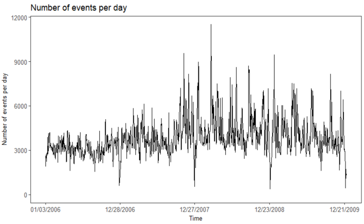
Figure 2: Event arrival rates (number of event-type mentions per day) for major banks.

8.2 Detection of structural changes during financial crisis

Next, we applied the non-parametric structural change detection algorithm NSA on the banking industry returns. The analysis was done as a multivariate run covering all banks simultaneously using $L_{1}$ norm as the regularization function $\varphi$. The regularization strength parameter $\gamma_{n}$ was selected using Bayesian information criterion. As a response variable $y_{t}=(r_{t}^{1},\dots,r_{t}^{10})\in\mathbb{R}^{10}$, we consider the log-returns of the 10 banks. As explanatory variables, we have $x_{t}=(v_{t},e_{t})\in\mathbb{R}^{591}$, where $v_{t}\in\mathbb{R}^{10}$ represents the bank-specific trading volumes and $e_{t}\in\mathbb{R}^{581}$ is the collection of event count indicators that have been extracted from Reuters news.

The results are shown in Figure 3. The multivariate statistic suggests 3 change points, which are located in the middle of May-2007, May-2008 and August-2008. When considering similar statistics for the individual banks, we see a bit more variation in number and location of changes, but they are, nevertheless, quite close to the ones detected by the multivariate statistic.

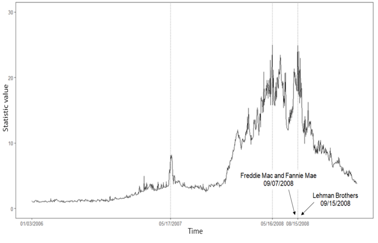
Figure 3: Multivariate energy-distance statistic. The dashed vertical lines indicate the locations of structural change points detected using bootstrap test statistics.

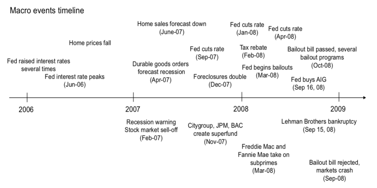
Figure 4: Macro-events timeline.

The macro-events timeline in Figure 4 gives rather natural explanations for the four regimes found by the multivariate statistic: (i) The first regime (01/03/2006 - 05/17/2007) can be interpreted as the escalation of subprime mortgage bubble into a recession. As home prices fell and Fed rates remained high, many homeowners couldn’t pay their mortgages, nor sell their homes for a profit. The high number of defaults caused the subprime mortgage crisis, which by March 2007 was spreading to the financial industry. (ii) The second regime (05/17-2007 - 05/16/2008) marks the period where the Fed finally takes action to curb the crisis through sequence of interest rate cuts and plans for bailout programs. (iii) However, despite the promising actions, the entire economy was already in recession during the third regime (05/16/2008 - 08/15/2008). This short and unstable regime soon ended as the mortgage giants Fannie Mae and Freddie Mac succumbed to the subprime crisis in August 2008. (iv) Their bankruptcy was soon followed by the cases of Lehman Brothers and AIG. To prevent the financial system from collapsing, the fourth regime (08/15/2008 - 01/01/2009) represents the period of massive bailout programs. For bank-specific analysis, see Appendix C.2.

As a disclaimer applying to this empirical example with financial data, it is important to note that there are nor ’right’ or ’wrong’ number of changes. Here, we have a used rather conservative settings, which allow detection of only substantial changes in the residual distributions. However, these settings can be naturally adjusted depending on the use case. For instance, analysts, who need early warning mechanisms, may want to use much higher detection sensitivity. As seen from Figure 3, the energy distance statistic shows many spikes that are not considered as structural changes under the current settings, but which could be really meaningful as early warning signals that could be utilized by traders and policy makers alike.

9 Conclusions

We have studied energy-distance based approaches for structural change detection in linear regression models. In particular, we consider models with multiple responses and potentially large number of explanatory variables. Our results show that already weak moment conditions on regressors and residuals are sufficient to ensure consistent estimation of structural change points. Furthermore, our simulation studies show that even under heavy-tailed errors or outlier contamination, both locations of structural change points and subsets of contributing variables can still be detected with high accuracy. Two alternative algorithms are suggested. The first algorithm is based on the use of dynamic programming principle to find the change points as global minimizers of the energy-distances between regime-wise residuals. The second algorithm is a heuristic, which combines nonparametric energy-distance with a computationally efficient splitting strategy. Though dynamic programming always leads to better detection accuracy, the heuristic came very close under most test configurations in the simulation studies. We also demonstrated the importance of regularization techniques in eliminating nuisance variables from the models and the subsequent impact on accuracy of structural change detection.

Appendix A: Technical proofs for consistency results

A.1. Proof (of Lemma 2)

Since

$$\frac{1}{n^{2}}\sum_{i_{1},i_{2}=1}^{n}X_{i_{1},i_{2}}-C=\frac{1}{n^{2}}\sum_{i_{1},i_{2}=1}^{n}(X_{i_{1},i_{2}}-C),$$

we can, without loss of generality, assume that $C=0$. Minkowski inequality implies that, for any $a>0$,

$$\mathbb{P}\left(\frac{1}{n^{2}}\left|\sum_{i_{1},i_{2}=1}^{n}X_{i_{1},i_{2}}\right|>a\right)\leq\frac{1}{n^{4}a^{2}}{\mathbb{E}}\left(\sum_{i_{1},i_{2}=1}^{n}X_{i_{1},i_{2}}\right)^{2}=\frac{1}{n^{4}a^{2}}\sum_{i_{1},i_{2},i_{3},i_{4}=1}^{n}{\mathbb{E}}\left[X_{i_{1},i_{2}}X_{i_{3},i_{4}}\right].$$

Denote

$$m=\min_{k,j\in\{1,2,3,4\},k\neq j}|i_{k}-i_{j}|.$$

By assumption, for each $\epsilon>0$, there exists $N$ such that $|{\mathbb{E}}\left[X_{i_{1},i_{2}}X_{i_{3},i_{4}}\right]|<\epsilon$ for any $m\geq N$. Write

$$\sum_{i_{1},i_{2},i_{3},i_{4}=1}^{n}{\mathbb{E}}\left[X_{i_{1},i_{2}}X_{i_{3},i_{4}}\right]=\sum_{i_{1},i_{2},i_{3},i_{4}=1,m<N}^{n}{\mathbb{E}}\left[X_{i_{1},i_{2}}X_{i_{3},i_{4}}\right]+\sum_{i_{1},i_{2},i_{3},i_{4}=1,m\geq N}^{n}{\mathbb{E}}\left[X_{i_{1},i_{2}}X_{i_{3},i_{4}}\right].$$

Since $m<N$ only if the distance between one of the pairs $(i_{k},i_{l})$ is less than $N$, we observe that the first term is bounded by

$$\sum_{i_{1},i_{2},i_{3},i_{4}=1,m<N}^{n}{\mathbb{E}}\left[X_{i_{1},i_{2}}X_{i_{3},i_{4}}\right]\leq D(N)n^{3}$$

for some finite constant depending only on $N$. For the second term, we estimate

$$\sum_{i_{1},i_{2},i_{3},i_{4}=1,m\geq N}^{n}|{\mathbb{E}}\left[X_{i_{1},i_{2}}X_{i_{3},i_{4}}\right]|<\epsilon n^{4}.$$

Combining the above bounds we obtain

$$\mathbb{P}\left(\frac{1}{n^{2}}\left|\sum_{i_{1},i_{2}=1}^{n}X_{i_{1},i_{2}}\right|>a\right)\leq\frac{D(N)}{na^{2}}+\frac{\epsilon}{a^{2}}.$$

Since $\epsilon>0$ is arbitrary, the result follows by choosing $n$ large enough.

Remark 2.

Note that, if

$$n^{-2}\sum_{i_{1},i_{2}=1}^{n}{\mathbb{E}}[X_{i_{1},i_{2}}]\rightarrow C,$$ (17)

then a slight modification of the above proof shows that $\frac{1}{n^{2}}\sum_{i_{1},i_{2}=1}^{n}X_{i_{1},i_{2}}\rightarrow C$ in probability, provided that $Cov(X_{i_{1},i_{2}},X_{i_{3},i_{4}})\rightarrow 0$ as $\min_{k,j\in\{1,2,3,4\},k\neq j}|i_{k}-i_{j}|\rightarrow\infty.$ Finally, we note that with similar arguments we obtain (17) provided that $\lim_{|i_{1}-i_{2}|\rightarrow\infty}|{\mathbb{E}}[X_{i_{1},i_{2}}]-C|=0.$

A.2. Proof (of Proposition 1)

The proof is by contradiction. Assume that $\lambda_{1}^{0}$ is not consistently estimated, i.e. $\hat{\lambda}_{1}\neq\lambda_{1}^{0}$. Without loss of generality, we assume that the estimated change point $\hat{T}_{1}$ satisfies $\hat{T}_{1}<T\lambda_{1}^{0}$, giving us a partitioning $I_{1}=[0,\hat{T}_{1}]$, $I_{2}=[\hat{T}_{1}+1,T_{1}^{0}]$ and $I_{3}=[T_{1}^{0}+1,T]$.

We denote by $|A|$ the size of a set $A$. In particular, we have that $|I_{1}\cup I_{2}\cup I_{3}|=T$, $|I_{3}|=(1-\lambda_{1}^{0})T$, $|I_{1}|\sim\hat{\lambda}_{1}T$, $|I_{2}|\sim(\lambda_{1}^{0}-\hat{\lambda}_{1})T$, and $|I_{2}\cup I_{3}|\sim(1-\hat{\lambda}_{1})T$ (where the notation $f(T)\sim g(T)$ refers to the usual interpretation $\lim_{T\to\infty}\frac{f(T)}{g(T)}=1$). For notational simplicity, we denote by $\hat{\beta}(i)$ the estimator corresponding to the region where $i$ belongs. That is, for $\hat{\beta}_{i},i=1,2$ denoting the regularized estimates, we have $\hat{\beta}(i)=\hat{\beta}_{1}$ for all $i\in I_{1}$, and $\hat{\beta}(i)=\hat{\beta}_{2}$ for all $i\in I_{2}\cup I_{3}$. Similarly, we denote by $\beta^{0}(i)$ the correct value corresponding to the region where $i$ belongs. That is, as the true change point is $T_{1}^{0}$, we have $\beta^{0}(i)=\beta^{0}_{1}$ for all $i\in I_{1}\cup I_{2}$ and $\beta^{0}(i)=\beta^{0}_{2}$ for all $i\in I_{3}$. We also denote by $\beta(i)$ and $\beta^{c}_{k}$ the limits related to Assumption 4. More precisely, we always have $\hat{\beta}(i)\rightarrow\beta(i)$ and $\hat{\beta}_{k}\rightarrow\beta^{c}_{k}$. Moreover, we have $\hat{\beta}(i)=\hat{\beta}_{1}\rightarrow\beta^{c}_{1}=\beta^{0}_{1}$ for all $i\in I_{1}$, as region $I_{1}$ is a subset of the correct interval $[0,T_{1}^{0}]$. For $i\in I_{2}\cup I_{3}$, we have $\hat{\beta}(i)=\hat{\beta}_{2}\rightarrow\beta^{c}_{2}$, and thus $\beta(i)=\beta^{c}_{2}$.

Denote by $\hat{u}_{i}=u_{i}-x_{i}^{\prime}(\hat{\beta}(i)-\beta^{0}(i)),i\in I_{k},k=1,2,3$ the corresponding estimated residuals and let $U_{1}=\{\hat{u}_{t}\}_{t\in I_{1}}$ and $U_{2}=\{\hat{u}_{t}\}_{t\in I_{2}\cup I_{3}}$ denote the collections of regularized residuals from different intervals. We set

$$\hat{\mu}^{\alpha}_{U_{1},U_{2}}=\frac{1}{|I_{1}||I_{2}\cup I_{3}|}\sum_{j\in I_{1},i\in I_{2}\cup I_{3}}|\hat{u}_{i}-\hat{u}_{j}|^{\alpha},\hat{\mu}^{\alpha}_{U_{1}}=\frac{1}{|I_{1}|^{2}}\sum_{i,j\in I_{1}}|\hat{u}_{i}-\hat{u}_{j}|^{\alpha},$$

and

$$\hat{\mu}^{\alpha}_{U_{2}}=\frac{1}{|I_{2}\cup I_{3}|^{2}}\sum_{i,j\in I_{2}\cup I_{3}}|\hat{u}_{i}-\hat{u}_{j}|^{\alpha}.$$

We prove that

$$2\hat{\mu}^{\alpha}_{U_{1},U_{2}}-\hat{\mu}^{\alpha}_{U_{1}}-\hat{\mu}^{\alpha}_{U_{2}}\rightarrow C>0,$$ (18)

where $C$ is a constant and the convergence holds in probability. From this we get

$$d_{\alpha}(U_{1},U_{2})=\frac{|I_{1}||I_{2}\cup I_{3}|}{2|I_{1}|+2|I_{2}\cup I_{3}|}\left(2\hat{\mu}^{\alpha}_{U_{1},U_{2}}-\hat{\mu}^{\alpha}_{U_{1}}-\hat{\mu}^{\alpha}_{U_{2}}\right)\rightarrow\infty.$$

Consequently, $\hat{T}_{1}$ cannot be a minimizer for the model equation 2 of Section 2 (in the paper), which leads to the expected contradiction.

We divide the rest of the proof into three steps. In step 1 we consider the differences $\hat{u}_{i}-\hat{u}_{j}$ that depend on the entire data set. In step 2 we calculate the limits of the terms $\hat{\mu}^{\alpha}_{U_{1},U_{2}}$, $\hat{\mu}^{\alpha}_{U_{1}}$, and $\hat{\mu}^{\alpha}_{U_{2}}$. Finally, in step 3, we show (18).

Step 1: We show that, for any subsets $A,B\subset\{1,2,\ldots,T\}$ we have

$$\begin{split}&\lim_{T\rightarrow\infty}\frac{1}{|A||B|}\sum_{i\in A,j\in B}|\hat{u}_{i}-\hat{u}_{j}|^{\alpha}\\ &=\lim_{T\rightarrow\infty}\frac{1}{|A||B|}\sum_{i\in A,j\in B}|u_{i}-u_{j}-x_{i}^{\prime}(\beta(i)-\beta^{0}(i))+x_{j}^{\prime}(\beta(j)-\beta^{0}(j))|^{\alpha},\end{split}$$

where the limits are understood in probability.
Recall that $\hat{u}_{i}=u_{i}-x_{i}^{\prime}(\hat{\beta}(i)-\beta^{0}(i))$ and denote

$$a_{ij}=\hat{u}_{i}-\hat{u}_{j}=u_{i}-x_{i}^{\prime}(\hat{\beta}(i)-\beta^{0}(i))-u_{j}+x_{j}^{\prime}(\hat{\beta}(j)-\beta^{0}(j)),$$ (19)

and

$$b_{ij}=u_{i}-x_{i}^{\prime}(\beta(i)-\beta^{0}(i))-u_{j}+x_{j}^{\prime}(\beta(j)-\beta^{0}(j)).$$ (20)

By writing

$$|a_{ij}|^{\alpha}=|b_{ij}|^{\alpha}+|a_{ij}|^{\alpha}-|b_{ij}|^{\alpha}$$

it suffices to prove that

$$\lim_{T\rightarrow\infty}\frac{1}{|A||B|}\sum_{i\in A,j\in B}||a_{ij}|^{\alpha}-|b_{ij}|^{\alpha}|\rightarrow 0$$

in probability. We now treat the case $\alpha\in(0,1]$ and $\alpha\in(1,2)$ separately.

Step 1.1: $\alpha\in(0,1]$.
By using the inequality $||a|^{\alpha}-|b|^{\alpha}|\leq||a|-|b||^{\alpha}\leq|a-b|^{\alpha}$, valid for all $a,b\in{\mathbb{R}}^{q}$ and $\alpha\in(0,1]$, for $a_{ij}$ and $b_{ij}$ we observe

$$||a_{ij}|^{\alpha}-|b_{ij}|^{\alpha}|\leq|a_{ij}-b_{ij}|^{\alpha}.$$

Here, by using $(|a|+|b|)^{\alpha}\leq|a|^{\alpha}+|b|^{\alpha}$, we obtain

$$\begin{split}|a_{ij}-b_{ij}|^{\alpha}&=|x^{\prime}_{i}(\beta(i)-\hat{\beta}(i))+x^{\prime}_{j}(\hat{\beta}(j)-\beta(j))|^{\alpha}\\ &\leq|x^{\prime}_{i}(\hat{\beta}(i))-\beta(i))|^{\alpha}+|x^{\prime}_{j}(\hat{\beta}(j)-\beta(j))|^{\alpha}\\ &\leq|x_{i}|^{\alpha}\quad||\hat{\beta}(i))-\beta(i)||^{\alpha}+|x_{j}|^{\alpha}\quad||\hat{\beta}(j))-\beta(j)||^{\alpha}.\end{split}$$

Since $\hat{\beta}(i)-\beta(i)=\hat{\beta}_{1}-\beta^{c}_{1}$ for $i\in I_{1}$ and $\hat{\beta}(i)-\beta(i)=\hat{\beta}_{2}-\beta^{c}_{2}$ for $i\in I_{2}\cup I_{3}$, we have

$$\begin{split}&\lim_{T\rightarrow\infty}\frac{1}{|A||B|}\sum_{i\in A,j\in B}|x_{i}|^{\alpha}\quad||\hat{\beta}(i))-\beta(i)||^{\alpha}\\ &=\lim_{T\rightarrow\infty}\frac{1}{|A|}\sum_{i\in A}|x_{i}|^{\alpha}\quad||\hat{\beta}(i))-\beta(i)||^{\alpha}\\ &=\lim_{T\rightarrow\infty}\frac{1}{|A|}\sum_{k=1}^{3}\sum_{i\in A\cap I_{k}}|x_{i}|^{\alpha}\quad||\hat{\beta}(i))-\beta(i)||^{\alpha}\\ &\leq\lim_{T\rightarrow\infty}\max_{k\in\{1,2\}}||\hat{\beta}_{k}-\beta^{c}_{k}||^{\alpha}\frac{1}{|A|}\sum_{i\in A}|x_{i}|^{\alpha}.\end{split}$$

Here the random variable

$$\frac{1}{|A|}\sum_{i\in A}|x_{i}|^{\alpha}$$

is uniformly bounded in $L^{1}$, and hence also in probability. Furthermore, we have

$$\max_{k\in\{1,2\}}||\hat{\beta}_{k}-\beta^{c}_{k}||^{\alpha}\rightarrow 0$$

in probability, and thus

$$\lim_{T\rightarrow\infty}\frac{1}{|A||B|}\sum_{i\in A,j\in B}|x_{i}|^{\alpha}\quad||\hat{\beta}(i))-\beta(i)||^{\alpha}\rightarrow 0.$$

Treating the term $|x_{j}|^{\alpha}\quad||\hat{\beta}(j))-\beta(j)||^{\alpha}$ similarly yields the claim.
Step 1.2: $\alpha\in(1,2)$.
We use the following inequality, valid for all $p\geq 0$ and $a,b\in{\mathbb{R}}^{q}$:

$$||a|^{p}-|b|^{p}|\leq\max(p,1)2^{(p-2)_{+}}\left[|a-b|^{p}+|b|^{(p-1)_{+}}|a-b|^{\min(p,1)}\right].$$

Plugging $p=\alpha$ together with $a_{ij}$ and $b_{ij}$ defined in equations (19) and (20) we have

$$||a_{ij}|^{\alpha}-|b_{ij}|^{\alpha}|\leq\alpha\left[|a_{ij}-b_{ij}|^{\alpha}+|b_{ij}|^{\alpha-1}|a_{ij}-b_{ij}|\right].$$ (21)

Jensen inequality implies

$$\begin{split}|a_{ij}-b_{ij}|^{\alpha}=&|x^{\prime}_{i}(\beta(i)-\hat{\beta}(i))+x^{\prime}_{j}(\hat{\beta}(j)-\beta(j))|^{\alpha}\\ \leq&2^{\alpha-1}\left[|x_{i}|^{\alpha}\quad||\hat{\beta}(i))-\beta(i)||^{\alpha}+|x_{j}|^{\alpha}\quad||\hat{\beta}(j))-\beta(j)||^{\alpha}\right].\end{split}$$

Now the first term on the right-hand side of (21) can be treated as in the case $\alpha\in(0,1)$. For the second term on the right-hand side of (21), we apply inequality $|a+b|^{\alpha-1}\leq|a|^{\alpha-1}+|b|^{\alpha-1}$ to estimate

$$\begin{split}|b_{ij}|^{\alpha-1}&=|u_{i}-x_{i}^{\prime}(\beta(i)-\beta^{0}(i))-u_{j}+x_{j}^{\prime}(\beta(j)-\beta^{0}(j))|^{\alpha-1}\\ &\leq|u_{i}|^{\alpha-1}+|x_{i}|^{\alpha-1}\quad||\beta(i))-\beta^{0}(i)||^{\alpha-1}+|u_{j}|^{\alpha-1}+|x_{j}|^{\alpha-1}\quad||\beta(j))-\beta^{0}(j)||^{\alpha-1}.\end{split}$$

Using this together with

$$|a_{ij}-b_{ij}|\leq|x_{i}|\quad||\hat{\beta}(i))-\beta(i)||+|x_{j}|\quad||\hat{\beta}(j))-\beta(j)||$$

and the fact that ${\mathbb{E}}|u|^{\alpha-1}\leq\left[{\mathbb{E}}|u|^{\alpha}\right]^{\frac{\alpha-1}{\alpha}}$, we obtain the claim by following similar steps as in the case $\alpha\in(0,1]$.

Step 2: We show that, for the limit $L$ defined by

$$L:=\lim_{T\rightarrow\infty}\left(2\hat{\mu}^{\alpha}_{U_{1},U_{2}}-\hat{\mu}^{\alpha}_{U_{1}}-\hat{\mu}^{\alpha}_{U_{2}}\right),$$

we have

$$\begin{split}L&=\frac{2(\lambda_{1}^{0}-\hat{\lambda}_{1})}{1-\hat{\lambda}_{1}}{\mathbb{E}}|U-\tilde{U}+X_{1}^{\prime}(\beta^{c}_{2}-\beta^{0}_{1})|^{\alpha}\\ &+\frac{2(1-\lambda_{1}^{0})}{1-\hat{\lambda}_{1}}{\mathbb{E}}|U-\tilde{U}-X_{2}^{\prime}(\beta^{c}_{2}-\beta^{0}_{2})|^{\alpha}-{\mathbb{E}}|U-\tilde{U}|^{\alpha}\\ &-\frac{(\lambda_{1}^{0}-\hat{\lambda}_{1})^{2}}{(1-\hat{\lambda}_{1})^{2}}{\mathbb{E}}|U-\tilde{U}+(\tilde{X}_{1}^{\prime}-X_{1}^{\prime})(\beta^{c}_{2}-\beta^{0}_{1})|^{\alpha}\\ &-\frac{(1-\lambda_{1}^{0})^{2}}{(1-\hat{\lambda}_{1})^{2}}{\mathbb{E}}|U-\tilde{U}+(\tilde{X}_{2}^{\prime}-X_{2}^{\prime})(\beta^{c}_{2}-\beta^{0}_{2})|^{\alpha}\\ &-2\frac{(1-\lambda_{1}^{0})(\lambda_{1}^{0}-\hat{\lambda}_{1})}{(1-\hat{\lambda}_{1})^{2}}{\mathbb{E}}|U-\tilde{U}-X_{2}^{\prime}(\beta^{c}_{2}-\beta^{0}_{2})+\tilde{X}_{1}^{\prime}(\beta^{c}_{2}-\beta^{0}_{1})|^{\alpha},\end{split}$$

where $U,\tilde{U}$ are independent copies of disturbances $u$ and $X_{i}^{\prime},\tilde{X}_{i}^{\prime}$ are independent copies drawn from the distribution of $X_{i}$ given in Assumption A2.
We study the limits of the terms $\hat{\mu}^{\alpha}_{U_{1},U_{2}}$, $\hat{\mu}^{\alpha}_{U_{1}}$, and $\hat{\mu}^{\alpha}_{U_{2}}$ separately. For the term $\hat{\mu}^{\alpha}_{U_{1}}$, as $\beta(i)=\beta^{0}(i)$ for all $i\in I_{1}$, we observe

$$\hat{\mu}^{\alpha}_{U_{1}}\rightarrow{\mathbb{E}}|U-\tilde{U}|^{\alpha}.$$

Consider next the term $\hat{\mu}^{\alpha}_{U_{1},U_{2}}$. Since $\beta(i)=\beta^{0}(i)$ for all $i\in I_{1}$, step 1 implies that it suffices to study the limit

$$\begin{split}&\lim_{T\rightarrow\infty}\frac{1}{|I_{1}||I_{2}\cup I_{3}|}\sum_{i\in I_{1},j\in I_{2}\cup I_{3}}|u_{i}-u_{j}+x_{j}^{\prime}(\beta(j)-\beta^{0}(j))|^{\alpha}\\ =&\lim_{T\rightarrow\infty}\frac{1}{|I_{1}||I_{2}\cup I_{3}|}\sum_{i\in I_{1},j\in I_{2}}|u_{i}-u_{j}+x_{j}^{\prime}(\beta(j)-\beta^{0}(j))|^{\alpha}\\ &+\lim_{T\rightarrow\infty}\frac{1}{|I_{1}||I_{2}\cup I_{3}|}\sum_{i\in I_{1},j\in I_{3}}|u_{i}-u_{j}+x_{j}^{\prime}(\beta(j)-\beta^{0}(j))|^{\alpha}.\end{split}$$

Recall that $\beta(j)=\beta^{c}_{2}$, $\beta^{0}(j)=\beta_{1}^{0}$, and $x_{j}\sim X_{1}$ for all $j\in I_{2}$. Since the proportion of observations is $\lambda_{1}^{0}-\hat{\lambda}_{1}$ in the regime $I_{2}$ and $1-\hat{\lambda}_{1}$ in the regime $I_{2}\cup I_{3}$, it now follows from Assumption 5 and Lemma 2, that

$$\lim_{T\rightarrow\infty}\frac{1}{|I_{1}||I_{2}\cup I_{3}|}\sum_{i\in I_{1},j\in I_{2}}|u_{i}-u_{j}+x_{j}^{\prime}(\beta(j)-\beta^{0}(j))|^{\alpha}=\frac{\lambda_{1}^{0}-\hat{\lambda}_{1}}{1-\hat{\lambda}_{1}}{\mathbb{E}}|U-\tilde{U}+X_{1}^{\prime}(\beta^{c}_{2}-\beta^{0}_{1})|^{\alpha}.$$

Similarly, as $\beta(j)=\beta^{c}_{2}$, $\beta^{0}(j)=\beta^{0}_{2}$, and $x_{j}\sim X_{2}$ for all $j\in I_{3}$, we observe that

$$\lim_{T\rightarrow\infty}\frac{1}{|I_{1}||I_{2}\cup I_{3}|}\sum_{i\in I_{1},j\in I_{3}}|u_{i}-u_{j}+x_{j}^{\prime}(\beta(j)-\beta^{0}(j))|^{\alpha}=\frac{1-\lambda_{1}^{0}}{1-\hat{\lambda}_{1}}{\mathbb{E}}|U-\tilde{U}-X_{2}^{\prime}(\beta^{c}_{2}-\beta^{0}_{2})|^{\alpha}.$$

It remains to study the limit of the term $\hat{\mu}^{\alpha}_{U_{2}}$. As above, we split

$$\{i\in I_{2}\cup I_{3},j\in I_{2}\cup I_{3}\}=\{i,j\in I_{2}\}\cup\{i,j\in I_{3}\}\cup\{i\in I_{2},j\in I_{3}\}\cup\{i\in I_{3},j\in I_{2}\}.$$

Similarly as above, we can apply Assumption 5 and Lemma 2 to obtain

$$\begin{split}&\lim_{T\rightarrow\infty}\frac{1}{|I_{2}\cup I_{3}|^{2}}\sum_{i,j\in I_{2}}|u_{i}-u_{j}-x_{i}^{\prime}(\beta(i)-\beta^{0}(i))+x_{j}^{\prime}(\beta(j)-\beta^{0}(j))|^{\alpha}\\ =&\frac{(\lambda_{1}^{0}-\hat{\lambda}_{1})^{2}}{(1-\hat{\lambda}_{1})^{2}}{\mathbb{E}}|U-\tilde{U}-X_{1}^{\prime}(\beta^{c}_{2}-\beta^{0}_{1})+\tilde{X}_{1}^{\prime}(\beta^{c}_{2}-\beta^{0}_{1})|^{\alpha},\end{split}$$

$$\begin{split}&\lim_{T\rightarrow\infty}\frac{1}{|I_{2}\cup I_{3}|^{2}}\sum_{i,j\in I_{3}}|u_{i}-u_{j}-x_{i}^{\prime}(\beta(i)-\beta^{0}(i))+x_{j}^{\prime}(\beta(j)-\beta^{0}(j))|^{\alpha}\\ =&\frac{(1-\lambda_{1}^{0})^{2}}{(1-\hat{\lambda}_{1})^{2}}{\mathbb{E}}|U-\tilde{U}-X_{2}^{\prime}(\beta^{c}_{2}-\beta^{0}_{2})+\tilde{X}_{2}^{\prime}(\beta^{c}_{2}-\beta^{0}_{2})|^{\alpha},\end{split}$$

$$\begin{split}&\lim_{T\rightarrow\infty}\frac{1}{|I_{2}\cup I_{3}|^{2}}\sum_{i\in I_{2},j\in I_{3}}|u_{i}-u_{j}-x_{i}^{\prime}(\beta(i)-\beta^{0}(i))+x_{j}^{\prime}(\beta(j)-\beta^{0}(j))|^{\alpha}\\ =&\frac{(1-\lambda_{1}^{0})(\lambda_{1}^{0}-\hat{\lambda}_{1})}{(1-\hat{\lambda}_{1})^{2}}{\mathbb{E}}|U-\tilde{U}-X_{1}^{\prime}(\beta^{c}_{2}-\beta^{0}_{1})+\tilde{X}_{2}^{\prime}(\beta^{c}_{2}-\beta^{0}_{2})|^{\alpha},\end{split}$$

and

$$\begin{split}&\lim_{T\rightarrow\infty}\frac{1}{|I_{2}\cup I_{3}|^{2}}\sum_{i\in I_{3},j\in I_{2}}|u_{i}-u_{j}-x_{i}^{\prime}(\beta(i)-\beta^{0}(i))+x_{j}^{\prime}(\beta(j)-\beta^{0}(j))|^{\alpha}\\ =&\frac{(1-\lambda_{1}^{0})(\lambda_{1}^{0}-\hat{\lambda}_{1})}{(1-\hat{\lambda}_{1})^{2}}{\mathbb{E}}|U-\tilde{U}-X_{2}^{\prime}(\beta^{c}_{2}-\beta^{0}_{2})+\tilde{X}_{1}^{\prime}(\beta^{c}_{2}-\beta^{0}_{1})|^{\alpha}.\end{split}$$

Observing

$${\mathbb{E}}|U-\tilde{U}-X_{1}^{\prime}(\beta^{c}_{2}-\beta^{0}_{1})+\tilde{X}_{2}^{\prime}(\beta^{c}_{2}-\beta^{0}_{2})|^{\alpha}={\mathbb{E}}|U-\tilde{U}-X_{2}^{\prime}(\beta^{c}_{2}-\beta^{0}_{2})+\tilde{X}_{1}^{\prime}(\beta^{c}_{2}-\beta^{0}_{1})|^{\alpha}$$

we obtain the claim.

Step 3: We show that for the limit $L$ defined in step 2, we have $L>0$.
By definition of the energy distance $\mathcal{E}(u,v;\alpha)$ for two random variables $u$ and $v$, we have that

$$\begin{split}\mathcal{E}(U,U+X_{1}^{\prime}(\beta^{c}_{2}-\beta^{0}_{1});\alpha)&=2{\mathbb{E}}|U-\tilde{U}+X_{1}^{\prime}(\beta^{c}_{2}-\beta^{0}_{1})|^{\alpha}-{\mathbb{E}}|U-\tilde{U}|^{\alpha}\\ &-{\mathbb{E}}|U-\tilde{U}+(\tilde{X}_{1}^{\prime}-X_{1}^{\prime})(\beta^{c}_{2}-\beta^{0}_{1})|^{\alpha},\end{split}$$

$$\begin{split}\mathcal{E}(U,U+X_{2}^{\prime}(\beta^{c}_{2}-\beta^{0}_{2});\alpha)&=2{\mathbb{E}}|U-\tilde{U}+X_{2}^{\prime}(\beta^{c}_{2}-\beta^{0}_{2})|^{\alpha}-{\mathbb{E}}|U-\tilde{U}|^{\alpha}\\ &-{\mathbb{E}}|U-\tilde{U}+(\tilde{X}_{2}^{\prime}-X_{2}^{\prime})(\beta^{c}_{2}-\beta^{0}_{2})|^{\alpha},\end{split}$$

and

$$\begin{split}\mathcal{E}(U+X_{2}^{\prime}(\beta^{c}_{2}-\beta^{0}_{2}),U+X_{1}^{\prime}(\beta^{c}_{2}-\beta^{0}_{1});\alpha)&=2{\mathbb{E}}|U-\tilde{U}+X_{1}^{\prime}(\beta^{c}_{2}-\beta^{0}_{1})-\tilde{X}_{2}^{\prime}(\beta^{c}_{2}-\beta^{0}_{2})|^{\alpha}\\ &-{\mathbb{E}}|U-\tilde{U}+(X_{1}^{\prime}-\tilde{X}_{1}^{\prime})(\beta^{c}_{2}-\beta^{0}_{1})|^{\alpha}\\ &-{\mathbb{E}}|U-\tilde{U}+(X_{2}^{\prime}-\tilde{X}_{2}^{\prime})(\beta^{c}_{2}-\beta^{0}_{2})|^{\alpha}.\end{split}$$

Moreover, we have that

$${\mathbb{E}}|U-\tilde{U}|^{\alpha}=\frac{\lambda_{1}^{0}-\hat{\lambda}_{1}}{1-\hat{\lambda}_{1}}{\mathbb{E}}|U-\tilde{U}|^{\alpha}+\frac{1-\lambda_{1}^{0}}{1-\hat{\lambda}_{1}}{\mathbb{E}}|U-\tilde{U}|^{\alpha},$$

$$\frac{\lambda_{1}^{0}-\hat{\lambda}_{1}}{1-\hat{\lambda}_{1}}-\frac{(\lambda_{1}^{0}-\hat{\lambda}_{1})^{2}}{(1-\hat{\lambda}_{1})^{2}}-\frac{(1-\lambda_{1}^{0})(\lambda_{1}^{0}-\hat{\lambda}_{1})}{(1-\hat{\lambda}_{1})^{2}}=0,$$

and

$$\frac{1-\lambda_{1}^{0}}{1-\hat{\lambda}_{1}}-\frac{(1-\lambda_{1}^{0})^{2}}{(1-\hat{\lambda}_{1})^{2}}-\frac{(1-\lambda_{1}^{0})(\lambda_{1}^{0}-\hat{\lambda}_{1})}{(1-\hat{\lambda}_{1})^{2}}=0.$$

These observations lead to

$$\begin{split}L&=\frac{\lambda_{1}^{0}-\hat{\lambda}_{1}}{1-\hat{\lambda}_{1}}\mathcal{E}(U,U+X_{1}^{\prime}(\beta^{c}_{2}-\beta^{0}_{1});\alpha)\\ &+\frac{1-\lambda_{1}^{0}}{1-\hat{\lambda}_{1}}\mathcal{E}(U,U+X_{2}(\beta^{c}_{2}-\beta^{0}_{2});\alpha)\\ &-\frac{(1-\lambda_{1}^{0})(\lambda_{1}^{0}-\hat{\lambda}_{1})}{(1-\hat{\lambda}_{1})^{2}}\mathcal{E}(U+X_{2}^{\prime}(\beta^{c}_{2}-\beta^{0}_{2}),U+X_{1}^{\prime}(\beta^{c}_{2}-\beta^{0}_{1});\alpha).\end{split}$$

Consequently, it suffices to prove that

$$\frac{\lambda_{1}^{0}-\hat{\lambda}_{1}}{1-\hat{\lambda}_{1}}\mathcal{E}(U,U+X_{1}^{\prime}(\beta^{c}_{2}-\beta^{0}_{1});\alpha)+\frac{1-\lambda_{1}^{0}}{1-\hat{\lambda}_{1}}\mathcal{E}(U,U+X_{2}^{\prime}(\beta^{c}_{2}-\beta^{0}_{2});\alpha)$$ (22)

$$-\frac{(1-\lambda_{1}^{0})(\lambda_{1}^{0}-\hat{\lambda}_{1})}{(1-\hat{\lambda}_{1})^{2}}\mathcal{E}(U+X_{2}^{\prime}(\beta^{c}_{2}-\beta^{0}_{2}),U+X_{1}^{\prime}(\beta^{c}_{2}-\beta^{0}_{1});\alpha) > 0.$$

Since $\mathcal{E}(u,v;\alpha)$ is a metric, triangle inequality implies that

$$\begin{split}\mathcal{E}(U+X_{2}^{\prime}(\beta^{c}_{2}-\beta^{0}_{2}),U+X_{1}^{\prime}(\beta^{c}_{2}-\beta^{0}_{1});\alpha)&\leq\mathcal{E}(U,U+X_{1}^{\prime}(\beta^{c}_{2}-\beta^{0}_{1});\alpha)\\ &+\mathcal{E}(U+X_{2}^{\prime}(\beta^{c}_{2}-\beta^{0}_{2}),U;\alpha).\end{split}$$

Furthermore, since $\beta^{0}_{1}\neq\beta^{0}_{2}$, we have that at least one of the terms $\mathcal{E}(U,U+X_{1}^{\prime}(\beta^{c}_{2}-\beta^{0}_{1});\alpha)$ and $\mathcal{E}(U,U+X_{2}^{\prime}(\beta^{c}_{2}-\beta^{0}_{2});\alpha)$ is strictly positive. We also observe that

$$\frac{(1-\lambda_{1}^{0})(\lambda_{1}^{0}-\hat{\lambda}_{1})}{(1-\hat{\lambda}_{1})^{2}}\leq\text{min}\left[\frac{\lambda_{1}^{0}-\hat{\lambda}_{1}}{1-\hat{\lambda}_{1}},\frac{1-\lambda_{1}^{0}}{1-\hat{\lambda}_{1}}\right],$$

and the inequality is strict whenever $\lambda_{1}^{0}<1$ and $\hat{\lambda}_{1}<\lambda_{1}^{0}$. As (22) is trivially valid for $\lambda_{1}^{0}=1$ or $\hat{\lambda}_{1}=\lambda_{1}^{0}$, this completes the proof.

A.3. Proof (of Proposition 2)

The proof is by contradiction. Assume that there exists one or more change points that are not consistently estimated. In order to prove the statement, it suffices to find two clusters $U_{i}$ and $U_{j}$ such that $d_{\alpha}(U_{j},U_{i})\rightarrow\infty$. Note first that there now exists at least one $j$ such that $T^{0}_{j-1}\leq\hat{T}_{j-1}<\hat{T}_{j}\leq T^{0}_{j}$. Consequently, there exists at least one cluster $U_{j}$ such that $\hat{\beta}_{j}\rightarrow\beta^{c}_{j}=\beta^{0}_{j}$. Similarly, there exists at least one index $i$ such that the open interval $(\hat{T}_{i-1},\hat{T}_{i})$ contains at least one true change point. Without loss of generality and for notational simplicity, we assume that $\hat{T}_{1}<T^{1}_{0}$ and that $(\hat{T}_{1},\hat{T}_{2})$ contains $m-1$ true change points $T^{0}_{1},T^{0}_{2},\ldots,T^{0}_{m-1}$, where $2\leq m\leq k+1$. As in the case of a single change point, we obtain a splitting $I_{1}=[1,\hat{T}_{1}]$, $I_{2}=[\hat{T}_{1}+1,T_{1}^{0}]$, $I_{3}=[T_{1}^{0}+1,T_{2}^{0}],\ldots,I_{m}=[T_{m-2}^{0}+1,T_{m-1}^{0}]$, and $I_{m+1}=[T_{m-1}^{0}+1,\hat{T}_{2}]$. Observe that the cluster $U_{1}$ corresponds to the time indexes contained in $I_{1}$ and that the cluster $U_{2}$ corresponds to the time indexes contained in $I=\cup_{j=2}^{m+1}I_{j}$. As in the case of a single change point, we also observe that $\beta(i)=\beta_{1}^{c}=\beta_{1}^{0}$ for each $i\in I_{1}$, and that $\beta(i)=\beta_{2}^{c}$ for each $i\in I$. However, the true values differ within intervals $I_{j}$ as, for $i\in I_{j}$, we have $\beta^{0}(i)=\beta_{j-1}^{0}$. Finally, we denote by $a_{j}$ the asymptotic proportions giving the amount of observations belonging to the intervals $I_{j}$. That is, we have $|I_{j}|\sim a_{j}T$.

As in the proof of Proposition 1, we set $\hat{u}_{i}=u_{i}-x_{i}^{\prime}(\hat{\beta}(i)-\beta^{0}(i))$, $U_{1}=\{\hat{u}_{t}\}_{t\in I_{1}}$ and $U=\{\hat{u}_{t}\}_{t\in I}$. It now suffices to prove that, for some constant $C>0$, we have

$$2\hat{\mu}^{\alpha}_{U_{1},U}-\hat{\mu}^{\alpha}_{U_{1}}-\hat{\mu}^{\alpha}_{U}\rightarrow C,$$ (23)

where

$$\hat{\mu}^{\alpha}_{U_{1},U}=\frac{1}{|I_{1}||I|}\sum_{j\in I_{1},i\in I}|\hat{u}_{i}-\hat{u}_{j}|^{\alpha},$$

$$\hat{\mu}^{\alpha}_{U_{1}}=\frac{1}{|I_{1}|^{2}}\sum_{i,j\in I_{1}}|\hat{u}_{i}-\hat{u}_{j}|^{\alpha},$$

and

$$\hat{\mu}^{\alpha}_{U}=\frac{1}{|I|^{2}}\sum_{i,j\in I}|\hat{u}_{i}-\hat{u}_{j}|^{\alpha}.$$

As the statement given in the step 1 of the proof of Proposition 1 holds for any subsets, we can directly proceed to computing the limits. The term $\hat{\mu}^{\alpha}_{U_{1}}$ can be treated as before, and we obtain

$$\lim_{T\rightarrow\infty}\hat{\mu}^{\alpha}_{U_{1}}={\mathbb{E}}|U-\tilde{U}|^{\alpha}.$$

For the term $\hat{\mu}^{\alpha}_{U_{1},U}$, we use $I=\cup_{j=2}^{m+1}I_{j}$. Now, for each subinterval $I_{j}$ separately, again by Assumption 5 and Lemma 2, we have that

$$\lim_{T\rightarrow\infty}\frac{1}{|I_{1}||I|}\sum_{i\in I_{1},j\in I_{j}}|u_{i}-u_{j}+x_{j}^{\prime}(\beta(j)-\beta^{0}(j))|^{\alpha}=\frac{a_{j}}{\sum_{k=2}^{m+1}a_{k}}{\mathbb{E}}|U-\tilde{U}+X_{j-1}^{\prime}(\beta^{c}_{2}-\beta^{0}_{j-1})|^{\alpha}.$$

Thus we obtain

$$\lim_{T\rightarrow\infty}\hat{\mu}^{\alpha}_{U_{1},U}=\sum_{j=2}^{m+1}\frac{a_{j}}{\sum_{k=2}^{m+1}a_{k}}{\mathbb{E}}|U-\tilde{U}+X_{j-1}^{\prime}(\beta^{c}_{2}-\beta^{0}_{j-1})|^{\alpha}.$$

Similarly, for the last term $\hat{\mu}_{U}^{\alpha}$, we have

$$\begin{split}&\lim_{T\rightarrow\infty}\frac{1}{|I|^{2}}\sum_{i\in I_{n_{1}},j\in I_{n_{2}}}|u_{i}-u_{j}-x_{i}^{\prime}(\beta(i)-\beta^{0}(i))+x_{j}^{\prime}(\beta(j)-\beta^{0}(j))|^{\alpha}\\ =&\frac{a_{n_{1}}a_{n_{2}}}{\left(\sum_{k=2}^{m+1}a_{k}\right)^{2}}{\mathbb{E}}|U-\tilde{U}-X_{n_{1}-1}^{\prime}(\beta^{c}_{2}-\beta^{0}_{n_{1}-1})+\tilde{X}_{n_{2}-1}^{\prime}(\beta^{c}_{2}-\beta^{0}_{n_{2}-1})|^{\alpha},\end{split}$$

leading to

$$\begin{split}\lim_{T\rightarrow\infty}\hat{\mu}_{U}^{\alpha}&=\sum_{n_{1},n_{2}=2}^{m+1}\frac{a_{n_{1}}a_{n_{2}}}{\left(\sum_{k=2}^{m+1}a_{k}\right)^{2}}{\mathbb{E}}|U-\tilde{U}-X_{n_{1}-1}^{\prime}(\beta^{c}_{2}-\beta^{0}_{n_{1}-1})+\tilde{X}_{n_{2}-1}^{\prime}(\beta^{c}_{2}-\beta^{0}_{n_{2}-1})|^{\alpha}.\end{split}$$

We proceed as in the step 3 of the proof of Proposition 1. By using the definition of energy distance, we have that, for any $i$ and $j$,

$$\begin{split}\mathcal{E}(U,U+X_{j}^{\prime}(\beta^{c}_{2}-\beta^{0}_{j});\alpha)&=2{\mathbb{E}}|U-\tilde{U}+X_{j}^{\prime}(\beta^{c}_{2}-\beta^{0}_{j})|^{\alpha}-{\mathbb{E}}|U-\tilde{U}|^{\alpha}\\ &-{\mathbb{E}}|U-\tilde{U}+(\tilde{X}_{j}^{\prime}-X_{j}^{\prime})(\beta^{c}_{2}-\beta^{0}_{j})|^{\alpha},\end{split}$$

and

$$\begin{split}\mathcal{E}(U+X_{j}^{\prime}(\beta^{c}_{2}-\beta^{0}_{j}),U+X_{i}^{\prime}(\beta^{c}_{2}-\beta^{0}_{i});\alpha)&=2{\mathbb{E}}|U-\tilde{U}+X_{i}^{\prime}(\beta^{c}_{2}-\beta^{0}_{i})-\tilde{X}_{j}^{\prime}(\beta^{c}_{2}-\beta^{0}_{j})|^{\alpha}\\ &-{\mathbb{E}}|U-\tilde{U}+(X_{i}^{\prime}-\tilde{X}_{i}^{\prime})(\beta^{c}_{2}-\beta^{0}_{i})|^{\alpha}\\ &-{\mathbb{E}}|U-\tilde{U}+(X_{j}^{\prime}-\tilde{X}_{j}^{\prime})(\beta^{c}_{2}-\beta^{0}_{j})|^{\alpha}.\end{split}$$

Together with the observation

$${\mathbb{E}}|U-\tilde{U}|^{\alpha}=\sum_{j=2}^{m+1}\frac{a_{j}}{\sum_{k=2}^{m+1}a_{k}}{\mathbb{E}}|U-\tilde{U}|^{\alpha},$$

and

$$\frac{a_{j}}{\sum_{k=2}^{m+1}a_{k}}-\frac{a^{2}_{j}}{\left(\sum_{k=2}^{m+1}a_{k}\right)^{2}}-\sum_{l=2,l\neq j}^{m+1}\frac{a_{l}a_{j}}{\left(\sum_{k=2}^{m+1}a_{k}\right)^{2}}=0$$

this leads to

$$\begin{split}&\lim_{T\rightarrow\infty}\left(\hat{\mu}_{U_{1},U}^{\alpha}-\hat{\mu}_{U_{1}}^{\alpha}-\hat{\mu}_{U}^{\alpha}\right)\\ &=\sum_{j=2}^{m+1}\frac{a_{j}}{\sum_{k=2}^{m+1}a_{k}}\mathcal{E}(U,U+X_{j-1}^{\prime}(\beta^{c}_{2}-\beta^{0}_{j-1});\alpha)\\ &-\sum_{n_{1},n_{2}=2,n_{1}\neq n_{2}}^{m+1}\frac{a_{n_{1}}a_{n_{2}}}{2\left(\sum_{k=2}^{m+1}a_{k}\right)^{2}}\mathcal{E}(U+X_{n_{1}-1}^{\prime}(\beta^{c}_{2}-\beta^{0}_{n_{1}-1}),U+X_{n_{2}-1}^{\prime}(\beta^{c}_{2}-\beta^{0}_{n_{2}-1});\alpha)\end{split}$$

which is positive by the arguments given in the step 3 of the proof of Proposition 1.

Appendix B: Methods used in the simulation study

In this section, we settings used for the test algorithms and their implementations. In a univariate case, we had 4 benchmarks: NPD, NSA, PSA, BP, ECP. PSA proposed by Gorskikh (2016), as well as NPD and NSA were implemented by us as an R code. BP (Bai and Perron, 1998, 2003) is available in an R-package ’strucchange’ (Zeileis, 2001). The ideas behind the implementation are described in Zeileis (2003). ECP (Matteson and James, 2014) is implemented in R package ’ecp’.

The settings for these methods were:

• BP: segment length $h$=50

• PSA: $\Theta=5$, $\theta=3$, $\Delta=50$, $\delta=20$ (which are correspondingly the number of contributing parameters and the length of segments at step 2 and 3)

• NSA: $\gamma=0.6$, $l=50$, $s=\tau=50$, $e=T-\tau=550$, $p_{0}=5\%$

• NDP (same as for NSA): $\tau=50$, $p_{0}=5\%$.

• ECP: $sig.lvl=5\%$, $\alpha=1$

For all methods, we select the minimum distance between change locations to be 50, which means that the maximum possible number of breaks detected will not exceed $T/\tau-1=11$.

In a multivariate case, we had 3 competing methods: NPD, NSA and QP. The first two methods (NPD and NSA) were implemented by us as an R code, whereas QP (Qu and Perron, 2007) is available as a GAUSS code at Pierre Perron’s homepage http://people.bu.edu/perron/.

The settings for these methods were:

• QP: m=11 (number of breaks allowed)

• NSA: $\gamma=0.6$, $l=50$, $s=\tau=50$, $e=T-\tau=550$, $p_{0}=5\%$

• NDP (same as for NSA): $\tau=50$, $p_{0}=5\%$.

Appendix C: Application to financial news analytics

C.1. News-event detection model

Fine-grained labeling tasks with thousands of categories are difficult to solve using a single classifier due to model capacity constraints and slow training speed (Ahmed et al. 2016; Gao et al. 2017). A common strategy to deal with this kind of problem is to divide output tags into semantically related subgroups (verticals) and train a specialist model per each subgroup separately. In our financial news analytics case, such strategy is relatively easy to implement, since there exists a natural taxonomy for organizing the events in a semantic hierarchy. For example, all fine-grained legal events can be grouped into one vertical while all outlook events can be grouped into another, and so on (see Figure 5). Each vertical may have a different number of output tags and also different amounts of training data. The overall model can then be represented as a tree-structured network with specialists representing branches. The choice of specialist is guided by a selector model (a course category classifier) that is optimized to discriminate the verticals.

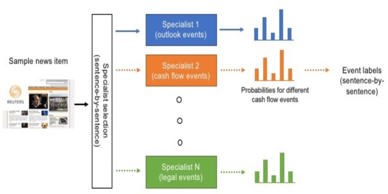
Figure 5: Multi-specialist network for event tagging

In our setup, each specialist network as well as the selector are modeled as bidirectional Long Short-Term Memory (LSTM) networks (Seo et al., 2016) with an attention mechanism (Figure 6). For simplicity, all event types considered in this study are assumed to be identifiable from sentence-level data. If identification of document-level events is needed, a hierarchical attention network can be considered (Yang et al., 2016).

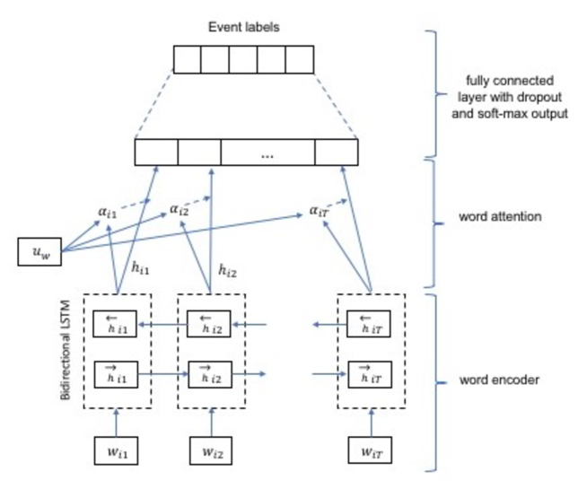
Figure 6: Bidirectional LSTM network with attention mechanism

As described in Figure 6, given a sentence with words $w_{it}$, $t\in[0,T]$, we first embed the words to vectors using a pre-trained embedding matrix $W_{e}$. The embeddings are then encoded using a standard bidirectional LSTM layer (Seo et al., 2016):

$$x_{it} = W_{e}w_{it},\ t\in[1,T]$$

$$\overrightarrow{h}_{it} = \overrightarrow{\text{LSTM}}(x_{it}),\ t\in[1,T]$$

$$\overleftarrow{h}_{it} = \overleftarrow{\text{LSTM}}(x_{it}),\ t\in[T,1]$$

The use of bidirectional LSTM summarizes information from both directions for words. The contextually enriched word encodings are then obtained by concatenating the forward and backward hidden states, i.e. $h_{it}=[\overrightarrow{h}_{it},\overleftarrow{h}_{it}]$. To extract words that are most relevant for the identifying the events in the sentence, this is followed by simple word attention mechanism (Yang et al., 2016) to compute importance weighted encodings. The normalized importance weights $\alpha_{it}$ are given by

$$u_{it} = \text{tanh}(W_{e}h_{it}+b_{w})$$

$$\alpha_{it} = \frac{\exp(u^{T}_{it}u_{w})}{\sum_{t}\exp(u^{T}_{it}u_{w})},$$

where $u_{it}$ is a hidden representation of $h_{it}$. As a final stage, the importance weighted word encodings are then passed to a fully connected layer with dropout and soft-max activation, which will then compute the probabilities for different event labels.

C.2. Bank-specific analysis of structural change points

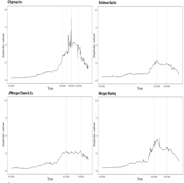
Figure 7: Bank-specific energy-distance statistics and structural change points. The dashed vertical lines indicate the locations of structural change points detected using bootstrap test statistics.

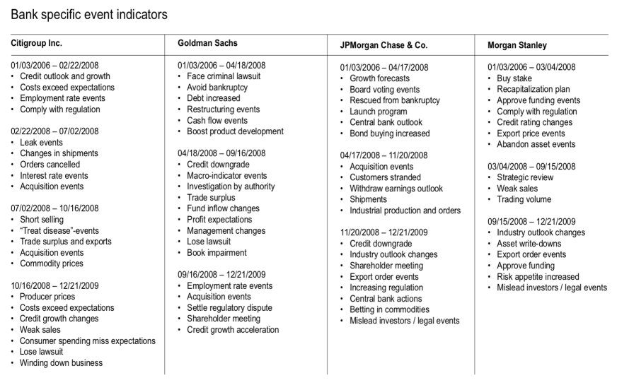
Figure 8: Collection of bank-specific event-type variables by regime.

Figures 7 and 8 provide more details on the regimes from the perspective of the individual banks. Notably, the general shape of the energy distance graphs in Figure 7 is relatively similar, and the variation in the number and length of regimes looks modest. For convenience, we show the energy-statistics only four banks, since the graphs of the remaining banks are very similar. In general, it looks like 2 or 3 structural change points are found. The multivariate statistic suggests 3 change points, which are located in the middle of May-2007, May-2008 and August-2008. When considering the statistics for the individual banks, we see a bit more variation in number and location of changes, but they are, nevertheless, quite close to the ones detected by the multivariate statistic. However, reflecting the unique state of each bank and the underlying dynamics of the economy, the subset of contributing event-indicators varies considerably across regimes as well as banks. Although, the overall number of possible event types was over 500 in the news wire dataset, the use of Lasso-regularization lead to rather sparse models with only 5-10 variables in each; see Figure 8. When considering the event types by regime, it appears that they agree quite well with the ones found by the multivariate statistic. However, in addition to macroeconomic events there are quite a lot of company specific legal issues, regulatory disputes, and news dealing with their restructuring and recapitalization plans.

References

• Abernethy et al. (2009) Abernethy, J., F. Bach, T. Evgeniou, and J.-P. Vert (2009). A new approach to collaborative filtering: Operator estimation with spectral regularization. Journal of Machine Learning Research 10, 803–826.
• Agarwal et al. (2012) Agarwal, A., S. Negahban, and M. J. Wainwright (2012, 04). Noisy matrix decomposition via convex relaxation: Optimal rates in high dimensions. Ann. Statist. 40(2), 1171–1197.
• Bai and Perron (1998) Bai, J. and P. Perron (1998). Estimating and testing linear models with multiple structural changes. Econometrica 66(1), 47–78.
• Bai and Perron (2003) Bai, J. and P. Perron (2003). Computation and analysis of multiple structural change models. Journal of Applied Econometrics 18(1), 1–22.
• Bellman and Roth (1969) Bellman, R. and R. Roth (1969). Curve fitting by segmented straight lines. Journal of the American Statistical Association 64, 111–125.
• Boudoukh et al. (2013) Boudoukh, J., R. Feldman, S. Kogan, and M. Richardson (2013, January). Which news moves stock prices? a textual analysis. Working Paper 18725, National Bureau of Economic Research.
• Cho and Fryzlewicz (2015) Cho, H. and P. Fryzlewicz (2015). Multiple-change-point detection for high dimensional time series via sparsified binary segmentation. Journal of the Royal Statistical Society: Series B (Statistical Methodology) 77(2), 475–507.
• Chopin (2006) Chopin, N. (2006). Dynamic detection of change points in long time series. The Institute of Statistical Mathematics, pp, 349–366.
• Davis et al. (2006) Davis, R., T. Lee, and G. Rodriguez-Yam (2006). Structural break estimation for nonstationary time series models. Journal of the American Statistical Association 101(473), 223–239.
• Fan et al. (2011) Fan, J., J. Lv, and L. Qi (2011). Sparse high-dimensional models in economics. Annual Review of Economics 3(1), 291–317.
• Fisher (1958) Fisher, W. D. (1958). On grouping for maximum homogeneity. Journal of the American Statistical Association 53, 789–798.
• Fryzlewicz (2014) Fryzlewicz, P. (2014, 12). Wild binary segmentation for multiple change-point detection. Ann. Statist. 42(6), 2243–2281.
• Gorskikh (2016) Gorskikh, O. (2016). Splitting algorithm for detecting structural changes in predictive relationships. In Advances in Data Mining. Applications and Theoretical Aspects. ICDM 2016. Lecture Notes in Computer Science, Cham, pp.  405–419. Springer.
• Groen et al. (2013) Groen, J., G. Kapetanios, and S. Price (2013). Multivariate methods for monitoring structural change. Journal of Applied Econometrics 28(2), 250–274.
• Harchaoui and Lévy-Leduc (2010) Harchaoui, Z. and C. Lévy-Leduc (2010). Multiple change-point estimation with a total variation penalty. Journal of the American Statistical Association 105(492), 1480–1493.
• Hariz et al. (2007) Hariz, S., J. Wylie, and Q. Zhang (2007, 08). Optimal rate of convergence for nonparametric change-point estimators for nonstationary sequences. Ann. Statist. 35(4), 1802–1826.
• Hoeffding (1961) Hoeffding, W. (1961). The strong law of large numbers for u-statistics. Technical report 302, North Carolina state University.
• Kanamori et al. (2009) Kanamori, T., S. Hido, and M. Sugiyama (2009, December). A least-squares approach to direct importance estimation. J. Mach. Learn. Res. 10, 1391–1445.
• Kawahara and Sugiyama (2012) Kawahara, Y. and M. Sugiyama (2012, April). Sequential change-point detection based on direct density-ratio estimation. Stat. Anal. Data Min. 5(2), 114–127.
• Koudijs (2016) Koudijs, P. (2016). The boats that did not sail: Asset price volatility in a natural experiment. The Journal of Finance 71(3), 1185–1226.
• Kurozumi and Arai (2007) Kurozumi, E. and Y. Arai (2007). Efficient estimation and inference in cointegrating regressions with structural change. Journal of Time Series Analysis 28(4), 545–575.
• Lavielle and Teyssière (2006) Lavielle, M. and G. Teyssière (2006). Detection of multiple change-points in multivariate time series. Lithuanian Mathematical Journal 46(3), 287–306.
• Lebarbier (2005) Lebarbier, E. (2005). Detecting multiple change-points in the mean of gaussian process by model selection. Signal Processing 85(4), 717 – 736.
• Li and Perron (2017) Li, Y. and P. Perron (2017). Inference on locally ordered breaks in multiple regressions. Econometric Reviews 36(1-3), 289–353.
• Liu et al. (2013) Liu, S., M. Yamada, N. Collier, and M. Sugiyama (2013). Change-point detection in time-series data by relative density-ratio estimation. Neural Networks 43, 72 – 83.
• Matteson and James (2014) Matteson, D. and N. James (2014). A nonparametric approach for multiple change point analysis of multivariate data. Journal of the American Statistical Association 109(505), 334–345.
• Negahban and Wainwright (2011) Negahban, S. and M. Wainwright (2011). Estimation of (Near) Low-Rank Matrices with Noise and High-Dimensional Scaling. The Annals of Statistics 39, 1069–1097.
• Qian and Su (2016) Qian, J. and L. Su (2016). Shrinkage estimation of regression models with multiple structural changes. Econometric Theory 32(6), 1376–1433.
• Qu and Perron (2007) Qu, Z. and P. Perron (2007). Estimating and testing structural changes in multivariate regressions. Econometrica 75(2), 459–502.
• Rizzo and Székely (2010) Rizzo, M. and G. J. Székely (2010). Disco analysis: A nonparametric extension of analysis of variance. The Annals of Applied Statistics 4(2), 1034–1055.
• Rizzo and Székely (2016) Rizzo, M. and G. J. Székely (2016). Energy distance. WIREs Comput Stat 8, 27–38.
• Ruggieri and Antonellis (2016) Ruggieri, E. and M. Antonellis (2016). An exact approach to bayesian sequential change point detection. Computational Statistics & Data Analysis 97, 71 – 86.
• Seo et al. (2016) Seo, M. J., A. Kembhavi, A. Farhadi, and H. Hajishirzi (2016). Bidirectional attention flow for machine comprehension. CoRR abs/1611.01603.
• Stock and Watson (2009) Stock, J. and M. Watson (2009). Forecasting in Dynamic Factor Models Subject to Structural Instability, pp.  1–57. Oxford University Press.
• Székely and Rizzo (2005) Székely, G. J. and M. Rizzo (2005). Hierarchical clustering via joint between-within distances: Extending ward’s minimum variance method. Journal of Classification 22(2), 151–183.
• Székely and Rizzo (2014a) Székely, G. J. and M. Rizzo (2014a). Energy statistics: A class of statistics based on distances. J. Statist. Plann. Inference 143, 1249–1272.
• Székely and Rizzo (2014b) Székely, G. J. and M. Rizzo (2014b). Partial distance correlation with methods for dissimilarities. The Annals of Statistics 42(6), 2382–2412.
• Yang et al. (2016) Yang, Z., D. Yang, C. Dyer, X. He, A. Smola, and E. Hovy (2016). Hierarchical attention networks for document classification. In Proceedings of the 2016 Conference of the North American Chapter of the Association for Computational Linguistics: Human Language Technologies, pp.  1480–1489. Association for Computational Linguistics.
• Yermack (2014) Yermack, D. (2014). Tailspotting: Identifying and profiting from ceo vacation trips. Journal of Financial Economics 113(2), 252 – 269.
• Yuan et al. (2007) Yuan, M., A. Ekici, Z. Lu, and R. Monteiro (2007). Dimension reduction and coefficient estimation in multivariate linear regression. Journal of the Royal Statistical Society: Series B (Statistical Methodology) 69(3), 329–346.
• Zeileis (2003) Zeileis, A., K. C. K. W. H. K. (2003). Testing and dating of structural changes in practice. Computational Statistics & Data Analysis 44, 109 – 123.
• Zeileis (2001) Zeileis, A., L. F. H. K. K. C. (2001). strucchange. An R package for testing for structural change in linear regression models. Technical report. SFB Adaptive Information Systems and Modelling in Economics and Management Science., WU Vienna University of Economics and Business.