Knowledge-based Fully Convolutional Network and Its Application in Segmentation of Lung CT Images

Abstract

A variety of deep neural networks have been applied in medical image segmentation and achieve good performance. Unlike natural images, medical images of the same imaging modality are characterized by the same pattern, which indicates that same normal organs or tissues locate at similar positions in the images. Thus, in this paper we try to incorporate the prior knowledge of medical images into the structure of neural networks such that the prior knowledge can be utilized for accurate segmentation. Based on this idea, we propose a novel deep network called knowledge-based fully convolutional network (KFCN) for medical image segmentation. The segmentation function and corresponding error is analyzed. We show the existence of an asymptotically stable region for KFCN which traditional FCN doesn’t possess. Experiments validate our knowledge assumption about the incorporation of prior knowledge into the convolution kernels of KFCN and show that KFCN can achieve a reasonable segmentation and a satisfactory accuracy.

1 Introduction

Medical image segmentation is of key importance for computer-aided diagnosis system. Accurate segmentation of healthy tissues and suspicious lesions is the basis of desired quantitative analysis of medical images. It is also very helpful for the research of various medical disorders. Quantification of structural variation by accurate measurement of volumes of region of interest can be used to evaluate severity of some disease or evolution of some tissues.

Recently it has been widely accepted that deep neural networks (DNN) have an impressive performance in various computer vision tasks. The techniques based on DNN have also been widely applied to the field of medical image segmentation and gain great success. The goal of segmentation with DNN is to allocate each pixel of the image with a corresponding category label. A lot of attempts have been made on dense pixel label prediction for medical images by developing various DNN. Brebisson et al. [1] use the CNNs for anatomical brain segmentation and achieve better performance. Zhang et al. [2] has proposed deep convolutional neural networks for extracting isointense stage brain tissues using multi-modality MR images. Li et al. [3] apply the CNNs to extract the intrinsic image features of lung image patches.

Long et al. [4] developed the Fully Convolutional Networks (FCN), which is implemented based on VGG-16 [5]. FCN is an end-to-end network, which can effectively solve the overstorage problem. He et al. [6] proposed deep residual network (ResNet), which efficiently combine information with extremely deep architectures and achieves compelling accuracy. Fisher et al. [7] proposed dilated convolution, which can effectively enlarge receptive field without losing resolution. It improves the performance in VGG-16 network and accelerate convergence. Ronneberger et al. [8] proposed U-Net for biomedical image segmentation. U-Net can be trained end-to-end from very few images. The architecture of U-Net consists of a contracting path to capture context and a symmetric expanding path that enables precise localization. Zhang et al. [9] proposed a pyramid dilated Res-U-Net based on ResNet and FCN with dilated residual unit. This net introduced LeakyReLU in the downsampling process and achieve desired performance for ultrasound nerve segmentation. Cui et al. [10] proposed a deep network based on ResNet and U-Net, which connected to a fully-connected CRF to refine boundary information.The pyramid dilated convolution is designed to exploit global context features with multi-scale.

Many great achievements have been made on various techniques of DNN for medical image segmentation. However, to our knowledge, so far the prior knowledge of the medical images has not been taken into consideration of the DNN-based approaches. Compared with natural images, medical images have a distinct feature: all images of the same imaging modality may contain same normal organs or tissues that are located at the similar positions in the images. This feature indicates that prior knowledge about organs or tissues is available in medical images, which can be utilized for coarse localization of these organs or tissues by registration methods. Most of current approaches based on deep nets train the kernel based on the information of whole images. Therefore the common features of similar but different structures may be learned in the medical images, such as the common features of left and right lungs in CT images. These features are useful for detecting and locating organs or tissues. But these global features may not be helpful for accurate segmentation of organs or tissues, which will be exemplified and analyzed in this paper.

In order to make full use of prior knowledge for accurate segmentation of medical images, we proposed a knowledge-based fully convolutional network in this paper. In this new framework, the medical images are pre-partitioned into different regions based on prior knowledge, each of which contain different organs or tissues. A strategy of knowledge-based convolution kernels is introduced into our KFCN such that our framework consists of multiple channels equipped with different convolution kernals that correspond to different regions. Instead of using information of whole image, in the KFCN model, each convolution kernel is trained with information only from the corresponding pre-partition region containing certain object. The difference between our strategy and current approaches is theoretically analyzed in section 2. Experiments about segmentation of lung CT images shows that our KFCN achieves better segmentation accuracy with the strategy of knowledge-based convolution kernels.

2 Method and Theory

Details of our knowledge based fully convolution network will be given in this section, along with some theoretical analysis of functions in KFCN and FCN. Some measurements necessary for our experiments to compare KFCN and FCN are given.

2.1 Prior knowledge

For most medical images, different objects tend to be organized in a similar way, confined to a similar bounded region in the image. For example, the left lung almost always locates on the left part of the image and the right lung on the right part. In this way, we can usually partition different objects into different boxes.

For an image segmentation task, we use $X$ to stand for the image variable. Then based on prior knowledge, we can partition it to be $X=(X_{1},X_{2},...,X_{n})$, where $X_{i}$ is part of $X$ and mainly contains one object, Also, we can segmentate this object in $X_{i}$ from the background without knowing the contents of $X_{j},~{}j\neq i$.

In traditional segmentation tasks, fully convoluional network (FCN) is adopted and in the convolutional layer of FCN, each convolutional kernel operates on all $X_{i}$. In other words, this convolutional layer can be formalized as

$$f(X;W)=(X_{1}*W,X_{2}*W,...,X_{n}*W),$$ (1)

where $W$ is the convolutional kernel and $*$ represents the convolution.

However, this kind of convolutional kernel will be affected by all objects and their features in the image. It will extract shared features of different objects and may miss some of their uniqueness, leading to poor segmentation performances.

In this paper, we attempt to incorporate prior knowledge of images about different objects into the design of convolutional layer, to construct convolutional kernels based on each kind of object. Specifically, instead of using the function in (1), we segmentate images with function

$$g(X;W)=(X_{1}*W_{1},X_{2}*W_{2},...,X_{n}*W_{n})$$ (2)

where $W$ could be seen as a kernel vector which contains a couple of convolutional kernels $W_{i},i=1,..,n$. In this way, each convolutional kernel is designed and trained for a specific object and feature. It turns out the kernel vector works more professional, and leads to better segmentation performances.

2.2 Knowledge-based FCN

Here we introduce the principle of constructing KFCN, for a segmentation task and images $\{X^{(i)}\}$, with the assumption that there are $n$ different objects in each image. At first, for image $X^{(i)}$, we apply a single shot multibox detector (SSD [11]) to get $n$ boxes $\{B^{(i)}_{j},j=1,...,n\}$ in image each mainly containing one object. Then, we extract data in these boxes out and resize them to have the same size, denoted as $\{Y^{(i)}_{j},j=1,...,n\}$. Next, we build $n$ independent small traditional FCN $N_{j},j=1,...,n$ with $N_{j}$ only deals with $Y^{(i)}_{j}$ to get $n+1$ probability maps $\{Z^{(i)}_{jk},k=1,..,n+1\}$, each represents the probability of pixels in $Y^{(i)}_{j}$ belonging to $n$ object class and the background class. Then we resize $\{\{Z^{(i)}_{jk},k=1,..,n+1\},j=1,..,n\}$ back to the size the original boxes $\{B^{(i)}_{j},j=1,...,n\}$ to get $\{\{U^{(i)}_{jk},k=1,..,n+1\},j=1,..,n\}$, each represents the probability of pixels in each box belonging to $n$ object class and the background class.

Then we make use an operation called sew up, for pixels in $X^{(i)}$ which lie in a box, from above process, we have got their probability map, for pixels outside of all boxes, we assume they all belong to the background, and thus can get their probability map, then we sew up these two parts together to get the probability map $\{V^{(i)}_{k},k=1,..,n+1\}$ of $X^{(i)}$.

Figure 1 gives a specific structure of KFCN which will be used in our following experiments based on lung CT images.

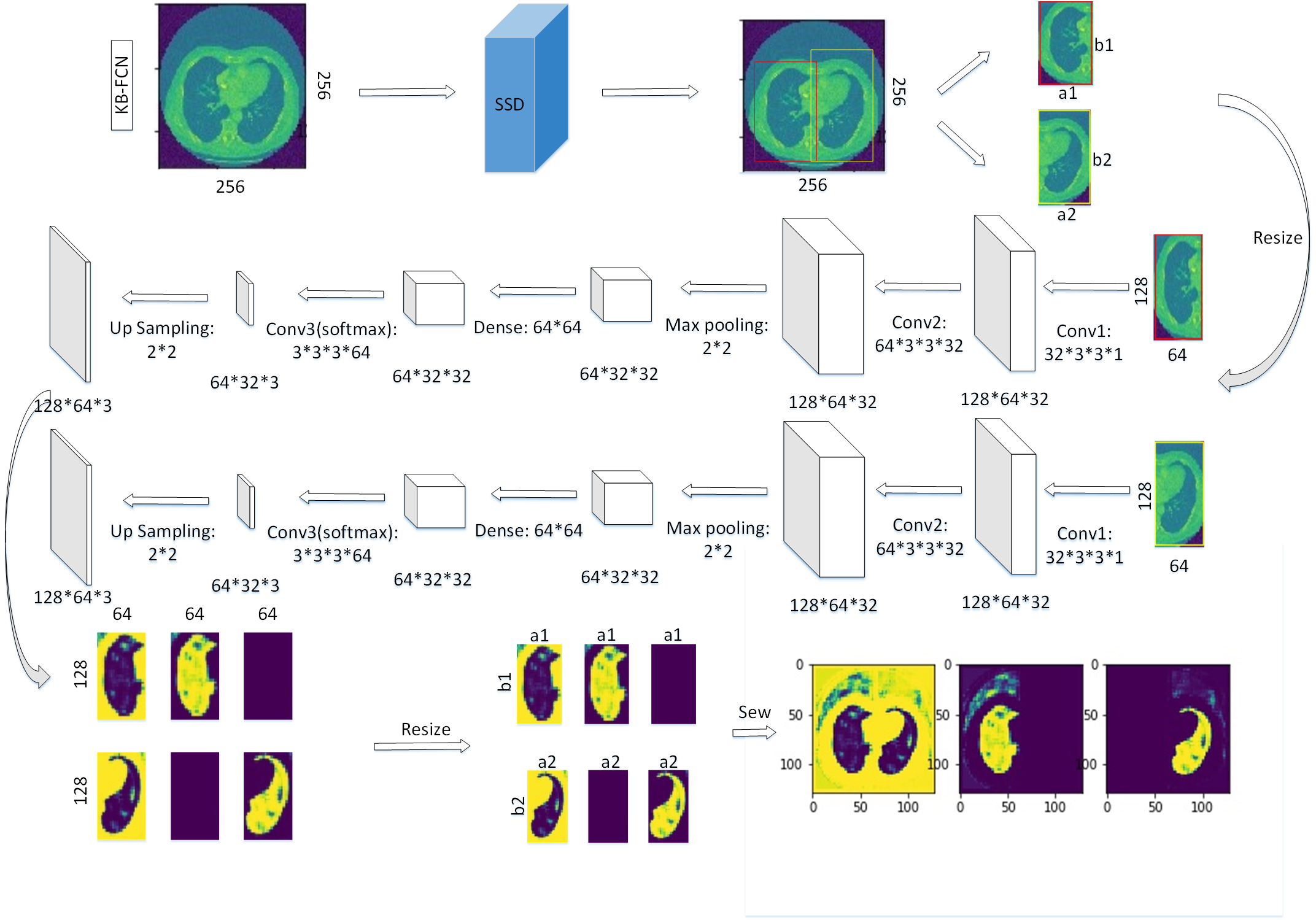
Figure 1: This is the structure of a KFCN used to segmentate lung CT images. On the first row, use a SSD to get the partition of images into boxes, then resize them into the fixed shape which were input to the next two channel, two small FCN in the second row. For each small FCN, it contains 6 layers, 3 convolution, 1 max pooling, 1 dense and 1 upsampling with specific size in the figure. In the third row, from two small FCN, we get probability maps and then resize them back to the size of original boxes, following a sew up operation to get the final probability maps of the image.

2.3 Analysis of functions in KFCN and FCN

In this subsection, we will evaluate the error of functions in kb-fcn and fcn in a simple settings. We consider only one convolutional layer based on ReLU as activation function. Without loss of generality, we may flatten one image variable $X$ to be a vector $\mathbf{x}$, where $\mathbf{x}=(\mathbf{x_{1}},\mathbf{x_{2}})$ is a $(d_{1}+d_{2})$ input data vector with $\mathbf{x_{1}}$ of length $d_{1}$, $\mathbf{x_{2}}$ of length $d_{2}$ which is a partition of $\mathbf{x}$, let $u=g(\mathbf{x},\mathbf{t^{*}})=(\mathbf{x_{1}}*\mathbf{t^{*}_{1}},\mathbf{x_{2}}*\mathbf{t^{*}_{2}})$ be the function which can accurately segmentate images with desired $(d_{3}+d_{4})$ output vector, where $\mathbf{t^{*}}=(\mathbf{t^{*}_{1}},\mathbf{t^{*}_{2}})$ are the vector form of convolutional kernels.

Then the function of KFCN can be formalized as $v_{1}=g(\mathbf{x},\mathbf{t})=(\mathbf{x_{1}}*\mathbf{t_{1}},\mathbf{x_{2}}*\mathbf{t_{2}})$, where $\mathbf{t}=(\mathbf{t_{1}},\mathbf{t_{2}})$ are the vector form estimator of convolutional kernels in KFCN. Comparatively the function of traditional fcn can be formalized as $v_{2}=g(\mathbf{x},\mathbf{t_{fc}})=(\mathbf{x_{1}}*\mathbf{t_{f}},\mathbf{x_{2}}*\mathbf{t_{f}})$, where $\mathbf{t_{fc}}=(\mathbf{t_{f}},\mathbf{t_{f}})$ are the vector form estimator of convolutional kernels in FCN.

As a matter of fact, we can write $\mathbf{x}*\mathbf{t}=\sigma(\mathbf{x}\mathbf{w})$, where $\sigma$ is the RELU function and $\mathbf{w}$ is the Toeplitz matrix of $\mathbf{t}$. We regard $\mathbf{w}$ as the changing variable. The next question would be to know that with $l_{2}$ loss $E_{1}(\mathbf{w_{1}})=||u-v_{1}||^{2}$ and $E_{2}(\mathbf{w_{fc}})=||u-v_{2}||^{2}$ (where $\mathbf{w_{1}},\mathbf{w_{fc}}$ are Toeplitz matrices of $\mathbf{t},\mathbf{t_{fc}}$), whether gradient descent will converge to the desired solution $\mathbf{w^{*}}=\mathbf{w_{t^{*}}}$. Note that the gradient descent update is $\mathbf{w^{(l+1)}}=\mathbf{w^{(l)}}+\eta\Delta\mathbf{w^{(l)}}$, where $\Delta\mathbf{w^{(l)}}=-\nabla E(\mathbf{w^{(l)}})$. Then, let $\eta\to 0$, we get that $\dot{\mathbf{w}}=-\nabla E(\mathbf{w})$, then $\dot{E}=-||\nabla E(\mathbf{w})||^{2}\leq 0$, the function value $E$ is nonincreasing. Hence, we need to check the points satisfying $\mathbf{w}\neq\mathbf{w^{*}}$ with $\nabla E(\mathbf{w})=0$.

In our analysis below, we take the assumption that entries of input $\mathbf{x}$ follow Gaussian distribution. In this situation, the gradient is a random variable and $\Delta\mathbf{w}=-\mathbf{E}[\nabla E(\mathbf{w})]$. The expected $\mathbf{E}[E(\mathbf{w})]$ is also nonincreasing no matter whether we follow the expected gradient or the gradient itself, for $\mathbf{\dot{E}}=\mathbf{E}[-\nabla E(\mathbf{w})^{T}\nabla E(\mathbf{w})]\leq-\mathbf{E}[\nabla E(\mathbf{w})]^{T}\mathbf{E}[\nabla E(\mathbf{w})]\leq 0$. Therefore, we analyze the behavior of expected gradient $\mathbf{E}[\nabla E(\mathbf{w})]$ rather than $\nabla E(\mathbf{w})$.

For simplicity, let $d_{1}=d_{2}=d,d_{3}=d_{4}=1$, then we have following lemma.

Lemma 1

(Lemma 3.1 in [12])

$$\mathbf{E}[\Delta\mathbf{w_{1}}]=\frac{1}{2}(\mathbf{w}^{*}-\mathbf{w_{1}})+\frac{1}{2\pi}(\frac{\mathbf{w}^{*}}{||\mathbf{w}^{*}||}\sin{\theta}\mathbf{w_{1}}-\theta\mathbf{w}^{*})\\$$ (3)

$$\mathbf{E}[\Delta\mathbf{w}_{fc}]=\frac{1}{2}(\mathbf{w}^{*}_{1}-\mathbf{w}_{f}+\mathbf{w}^{*}_{2}-\mathbf{w}_{f})+\frac{1}{2\pi}(\frac{\mathbf{w}^{*}_{1}}{||\mathbf{w}^{*}_{1}||}\sin{\theta_{1}}\mathbf{w}_{f}-\theta_{1}\mathbf{w}^{*}_{1}+\frac{\mathbf{w}^{*}_{2}}{||\mathbf{w}^{*}_{2}||}\sin{\theta_{2}}\mathbf{w}_{f}-\theta_{2}\mathbf{w}^{*}_{2})$$ (4)

where $\theta,\theta_{1},\theta_{2}\in[0,\pi]$ are the angles of $\mathbf{w},\mathbf{w}^{*}$, $\mathbf{w}_{f},\mathbf{w}^{*}_{1}$ and $\mathbf{w}_{f},\mathbf{w}^{*}_{2}$.

Combined with following lemma, we can arrive a good conclusion about the first function, which corresponds to the function in KFCN.

Lemma 2

(Lemma 3.2 in [12])

When $\mathbf{w}_{1}^{(1)}\in\Omega=\{\mathbf{w}:||\mathbf{w}-\mathbf{w}^{*}||<||\mathbf{w}^{*}||\}$, following the dynamics of $\mathbf{E}[\Delta\mathbf{w}_{1}]$, the Lyapunov function $V(\mathbf{w}_{1})=\frac{1}{2}||\mathbf{w}_{1}-\mathbf{w}^{*}||^{2}$ has $\dot{V}\leq 0$ the system is asymptotically stable and thus $\mathbf{w}_{1}^{(t)}\to\mathbf{w}^{*}$ when $t\to+\infty$

This ensures the convergence and correctness of our model by making use of prior knowledge. However, we would like to see what’s the situation for the second function corresponding to traditional FCN. Note that

$$\dot{V}=(\mathbf{w}_{f}-\mathbf{w}^{*}_{1})^{T}\Delta\mathbf{w}_{f}+(\mathbf{w}_{f}-\mathbf{w}^{*}_{2})^{T}\Delta\mathbf{w}_{f}$$ (5)

hence, we get $\dot{V}=-\mathbf{y}^{T}M\mathbf{y}$, where $\mathbf{y}=[||\mathbf{w}^{*}_{1}||,||\mathbf{w}^{*}_{2}||,||\mathbf{w}_{f}||]^{T}$ and $M$ is the following 3-by-3 matrix:

$$M=\frac{1}{4\pi}\left[\begin{array}[]{ccc}\sin(2\theta_{1})+2\pi-2\theta_{1}&(2\pi-\theta_{1}-\theta_{2})\cos(\alpha)+\sin(\theta_{1}+\theta_{2})\\ (2\pi-\theta_{1}-\theta_{2})\cos(\alpha)+\sin(\theta_{1}+\theta_{2})&\sin(2\theta_{2})+2\pi-2\theta_{2}\\ -(2\pi-\theta_{1})\cos(\theta_{1})-\sin(\theta_{1})&-(2\pi-\theta_{2})\cos(\theta_{2})-\sin(\theta_{2})\\ \end{array}\right.\\ \left.\begin{array}[]{cc}-(2\pi-\theta_{1})\cos(\theta_{1})-\sin(\theta_{1})\\ -(2\pi-\theta_{2})\cos(\theta_{2})-\sin(\theta_{2})\\ -4\pi\\ \end{array}\right]$$ (6)

where $\alpha\in[0,\pi]$ is the angle between $\mathbf{w}^{*}_{1}$ and $\mathbf{w}^{*}_{2}$.

Then we consider the conditions $\theta_{1},\theta_{2}$ should satisfy so as to find an asymptotically stable region, that is, $M$ should be positive definite in this region. It follows that all order principal minor determinant $D_{11},D_{22},D_{33}$ should be positive. Because of the complexity of the expression, we solve the equation numerically. The result turns out that for any $\alpha\in[0,\pi]$, there is no region where $\theta_{1},\theta_{2}\in[0,\pi]$ for $M$ to be positive definite. Consequently, there is no asymptotically stable region in this case.

Furthermore, when $d_{3},d_{4}$ become larger, the system becomes complicated and it is hard for us to analyze both cases, yet from theorem 4.1 in [12] , for the first function, we can still find an asymptotically stable region. Hence, from this analysis, we see the advantage of KFCN, since it represents a function with an asymptotically stable region, while traditional FCN represents a function doesn’t necessarily correspond to an asymptotically stable region.

2.4 Generalization ability and Similarity analysis

We will check our assumption that convolutional kernels which were used to segmentate different objects with high accuracy are different by considering the generalization ability of convolutional kernels. Generally speaking, we consider the performance of convolutional kernels trained based on one object when they were used to segmentate other objects.

Let $N_{i},N_{j}$ be two small FCN embedded in KFCN, for the generalition ability of convolutional kernels in $N_{i}$, we set the values of convolutional kernels in $N_{j}$ to be the values of convolutional kernels in $N_{i}$, and then do segmentation again to see the results, namely, segmentation performance, accuracy and loss.

By considering generalization ability of convolutional kernels, we can directly see the different performances caused by knowledge based convolutional kernels. However, it remains to be shown how similar and different these kernels are, which we will measure with the help of point-wise similarity of two couples of convolutional kernels.

Definition 1

For two convolutional kernels $w_{i}$ and $w^{\prime}_{j}$, their point-wise similarity is defined as

$$Sim(w_{i},w^{\prime}_{j})=\frac{w^{v}_{i}*w^{\prime v}_{j}}{||w^{v}_{i}||*||w^{\prime v}_{j}||}$$ (7)

where $w^{v}_{i},w^{\prime v}_{j}$ is the vector form of $w_{i},w^{\prime}_{j}$.

Definition 2

Let $\{w_{i}\}_{i=1}^{K}$ and $\{w^{\prime}_{j}\}_{j=1}^{K}$ be two couples of convolutional kernels. Rearrange $\{w^{\prime}_{j}\}_{j=1}^{K}$ such that $Sim(w_{i},w^{\prime}_{i})=\max_{j=1}^{K}Sim(w_{i},w^{\prime}_{j})$. Point-wise similarity of $\{w_{i}\}_{i=1}^{K}$ with respect to $\{w^{\prime}_{j}\}_{j=1}^{K}$ is defined as

$$Sim_{l}(\{w_{i}\}_{i=1}^{K},\{w^{\prime}_{j}\}_{j=1}^{K})=\frac{1}{K}\sum_{i=1}^{K}Sim(w_{i},w^{\prime}_{i})$$ (8)

Similarly, point-wise similarity $Sim_{r}(\{w_{i}\}_{i=1}^{K},\{w^{\prime}_{j}\}_{j=1}^{K})$ of $\{w^{\prime}_{j}\}_{j=1}^{K}$ with respect to $\{w_{i}\}_{i=1}^{K}$ can be derived in the same way.

Definition 3

Let $\{w_{i}\}_{i=1}^{K}$ and $\{w^{\prime}_{j}\}_{j=1}^{K}$ be two couples of convolutional kernels. Point-wise similarity of $\{w_{i}\}_{i=1}^{K}$ and $\{w^{\prime}_{j}\}_{j=1}^{K}$ is defined as

$$Sim(\{w_{i}\}_{i=1}^{K},\{w^{\prime}_{j}\}_{j=1}^{K})=\frac{1}{2}(Sim_{l}+Sim_{r})$$ (9)

We will calculate these values in our experiments so as to measure the similarity of several couples of convolutional kernels.

3 Experiments and Discussion

3.1 KFCN vs FCN

Based on a dataset on lung ct images with 246 images, we train a KFCN of the structure described in Figure 1. The baseline model is a traditional FCN with contains 6 layers, 3 convolution, 1 max pooling, 1 dense and 1 upsampling with the same size of the small FCN in Figure 1, trained on the same dataset. Figures 2 are the accuracy and loss curves of two networks on training set and validation set during training.

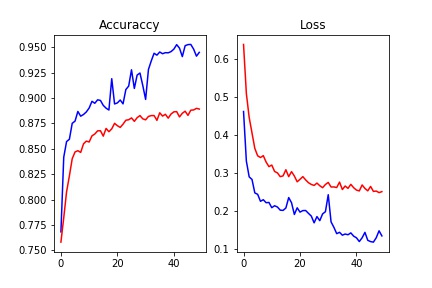
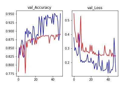
Figure 2: The left part are curves in training set, the right part are curves in validation set. Blue curves represents KFCN while red curves represents baseline FCN.

Also, the accuracy and loss of two models on original test set is shown in the left part of table 1, where the loss is calculated as mean squard error.

Table 1: Accuracy and loss on test set

Image	Original images		Flip images
Property	Accuracy	Loss	Accuracy	Loss
KFCN	$95.6\%$	0.022	$77.5\%$	0.125
FCN	$89.1\%$	0.048	$80.6\%$	0.129

Moreover, for an example of lung CT image, shown in Figure 3, where the left image is the original training image, the middle image is the ground truth of left lung and the right image is the ground truth of the right lung.

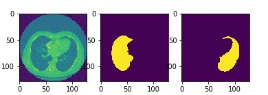
Figure 3: Original lung CT image and its ground truth

we show the corresponding segmentation by KFCN and traditional FCN respectively in figure 4, the first 2 images were segmentation of left lung and right lung by KFCN and the last 2 images were segmentation by traditional FCN.

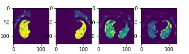
Figure 4: Segmentatation of images by KFCN and FCN

As you can see, KFCN and FCN are segmentating lungs in a different way. With knowledge based convolutional kernels, KFCN can extract different features and achieve a remarkable accuracy. On the other hand, though traditional FCN achieves a pretty high accuracy, its segmentations are not accurate and reasonable actually. Convolutional kernels in traditional FCN were affected by both features and can not distingunish different features well, which leads to a bad performance.

3.2 Generalization ability

Now we turn to consider the generalition ability of different knowledge based convolutional kernels. For generalization ability of convolutional kernels trained only on the left lung in KFCN, we apply them to do segmentation of the right lung. Conversely, the generalization ability of convolutional kernels trained only on the right lung in KFCN. Similarly, the generalization ability of convolutional kernels in FCN is taken into account. Actually, for lung CT images, we can just flip the left part and right part to get the same effect.

The segmentation of flip image of figure3 by two models is shown in Figure 5.

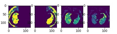
Figure 5: The first image is the segmentation when right kernels in KFCN were used to segmentate the left lung, the second image is the segmentation when left kernels in KFCN were used to segmentate the right lung. The last two images are the segmentation of kernels in FCN to the same flip image.

In this case, accuray and loss of KFCN and FCN were shown in the right part of table 1. It can be seen that convolutional kernels in KFCN have poor generality ability since they are specialized according to different objects, finding different features. However, convolutional kernels in traditional FCN have good generalition ability, extracting features shared by different objects. As a matter of fact, since these kernels operate on all image, so the segmentations vary a little compared to the segmentation of original image. So, These convolutional kernels which are to segmentate different objects with high accuracy are different to some extent while traditional FCN will ignore this prior knowledge.

3.3 Similarity analysis

We now have three couples of convolutional kernels with the same size, namely, $W_{L}=\{w_{l_{i}}\}_{i=1}^{n}$, convolutional kernels trained in KFCN operating on the left lung, $W_{R}=\{w_{r_{i}}\}_{i=1}^{n}$, convolutional kernels trained in KFCN operating on the right lung, $W_{T}=\{w_{t_{i}}\}_{i=1}^{n}$, convolutional kernels trained in traditional FCN operating on the whole image. The point wise similarity of them is calculated in table 2.

Table 2: Point-wise similarity

layer	kernels	$Sim_{l}$	$Sim_{r}$	$Sim$
$C_{1}$	$W_{L},W_{R}$	0.6908	0.6902	0.6905
	$W_{L},W_{T}$	0.8633	0.8518	0.8576
	$W_{R},W_{T}$	0.6630	0.6885	0.6758
$C_{2}$	$W_{L},W_{R}$	0.2550	0.2548	0.2549
	$W_{L},W_{T}$	0.2805	0.2757	0.2781
	$W_{R},W_{T}$	0.2395	0.2384	0.2390
$C_{3}$	$W_{L},W_{R}$	0.1536	0.1428	0.1482
	$W_{L},W_{T}$	0.1115	0.0865	0.0990
	$W_{R},W_{T}$	0.0692	0.1054	0.0873

It can be seen that only on the first layer, these kernels are similar, in the following layers, convolutional kernels vary a lot and have little in common. As a matter of fact, in the first layer, both networks are extracting similar basic features, what’s more, convolutional kernels in traditional FCN are similar to the convolutional kernels in KFCN in the first layer, yet in the following layers, these features are organized differently depends on different objects.

4 Conclusion

In this paper, we proposed a novel framework KFCN for medical image segmentation by incorporating prior knowledge into the design and training of convolutional kernels. Based on theoretical analysis of functions and error in KFCN and traditional FCN, we conclude that KFCN has an asymptotically stable region while traditional FCN does not necessarily do. This discovery demonstrates the convergence superiority of KFCN, which can converge asymptotically under mild conditions. Meanwhile, experimental results show that KFCN outperforms traditional FCN in segmentation of lung CT images. Furthermore, the numerical results about difference among convolutional kernels in terms of generalization ability and point-wise similarity, validates our assumption about incorporation of prior knowledge into KFCN, and illustrates the advantages of our knowledge-based convolutional kernels. In the future research, we will test KFCN for segmentation of various medical images and try to introduce KFCN framework into semantic segmentation of natural images. Another interesting research topic is to see the number of images required for KFCN to achieve a high accuracy.

References

[1] Brebisson, A.D. & Mountana, G. (2015) Deep neural networks for anatomical brain segmentation. Proceedings of the IEEE Conference on Computer Vision and Pattern Recognition Workshops.

[2] Zhang, W. Li, R., Deng, H. & Wang, L. (2015) Deep convolutional neural networks for multi-modality isointense infant brain image segmentation. NeuroImage108, pp.  214-224.

[3] Li, Q., Cai, T., Wang, X., Zhou, Y. & Feng, D. (2014) Medical image classification with convolutional neural network. the 13th International Conference on Control Automation Robotics & Vision (ICARCV). IEEE

[4] Long, J., Shelhamer, E. & Darrell, T. (2015) Fully convolutional networks for semantic segmentation. Proceedings of the IEEE Conference on Computer Vision and Pattern Recognition

[5] Simonyan, K. & Zisserman, A. (2014) Very deep convolutional networks for large-scale image recognition[J]. ArXiv preprint arXiv:1409.1556

[6] He, K., Zhang, X., Ren, S. & Sun, J. (2016) Deep residual learning for image recognition. Proceedings of the Institute of Electrical and Electronics Engineers Conference on Computer Vision and Pattern Recognition

[7] Yu, F. & Koltun, V. (2015) Multi-scale context aggregation by dilated convolutions. ArXiv preprint arXiv:1511.07122

[8] Ronneberger, O., Fischer, P. & Brox, T. (2015) U-net: Convolutional networks for biomedical image segmentation[C]. International Conference on Medical Image Computing and Computer-Assisted Intervention. pp. 234-241. Springer, Cham.

[9] Zhang, Q., Cui, Z., Niu, X., Geng, S. & Qiao, Y. (2017) Image Segmentation with Pyramid Dilated Convolution based on ResNet and U-Net. 24th International Conference on Neural Information Processing

[10] Cui, Z., Zhang, Q., Geng, S., Niu, X., Yang, J. & Qiao, Y. (2017) Semantic Segmentation with Multi-path Refinement and Pyramid Pooling Dilated-Resnet. 2017 IEEE International Conference on Image Processing

[11] Liu, W., Anguelov2, D., Erhan3, D., Szegedy3, C., Reed4, S., Fu, C., Alexander C. Berg1 (2016) SSD: Single Shot MultiBox Detector. European Conference on Computer Vision

[12] Tian, Y. (2017) Symmetry-breaking convergence analysis of certain two-layered neural networks with RELU nonlinearity. International Conference on Learning Representations