Distributed Partitioned Big-Data Optimization
via Asynchronous Dual Decomposition

Abstract

In this paper we consider a novel partitioned framework for distributed optimization in peer-to-peer networks. In several important applications the agents of a network have to solve an optimization problem with two key features: (i) the dimension of the decision variable depends on the network size, and (ii) cost function and constraints have a sparsity structure related to the communication graph. For this class of problems a straightforward application of existing consensus methods would show two inefficiencies: poor scalability and redundancy of shared information. We propose an asynchronous distributed algorithm, based on dual decomposition and coordinate methods, to solve partitioned optimization problems. We show that, by exploiting the problem structure, the solution can be partitioned among the nodes, so that each node just stores a local copy of a portion of the decision variable (rather than a copy of the entire decision vector) and solves a small-scale local problem.

I Introduction

Distributed optimization has received a widespread attention in the last years due to its key role in multi-agent systems (also known as large-scale systems, sensor networks or peer-to-peer networks). Several solutions have been proposed, but many challenges are still open. In this paper we focus on a main common limitation of the current approaches. That is, in all the currently available algorithms the nodes in the network reach consensus on the entire solution vector. This redundancy of information may be not necessary or even realizable in some problem set-ups. Thus, we exploit a new distributed optimization set-up in which the nodes compute only a portion of the solution and the whole minimizer may be obtained by stacking together the local portions.

We divide the relevant literature for our paper in two parts. That is, we review works on distributed optimization more closely related to the techniques proposed in this paper, and the centralized and parallel literature on big-data optimization.

Early references on distributed optimization are [2, 3]. Convex optimization problems are solved by using a primal distributed subgradient method combined with a consensus scheme. Dual decomposition methods have been proposed in early references in order to develop distributed algorithms in a pure peer-to-peer set-up. In [4] a tutorial on network optimization via dual decomposition can be found. In [5] a synchronous distributed algorithm based on a dual decomposition approach is proposed for a convex optimization problem with a common constraint for all the agents. In [6] equality and inequality constraints are handled in a distributed set-up based on duality. In [7] a distributed algorithm based on an averaging scheme on the dual variables is proposed, to solve convex optimization problems over fixed undirected networks. A slightly different set-up is considered in [8], where a dual decomposition method over time-varying graphs is proposed. In order to induce robustness in the computation and improve convergence in the case of non-strictly convex functions, Alternating Direction Methods of Multipliers (ADMM) have been proposed in the network context [9]. A distributed consensus optimization algorithm based on an inexact ADMM is proposed in [10]. In [11] an asynchronous ADMM-based distributed method is proposed for a separable, constrained optimization problem. A different class of algorithms, working under a general asynchronous and directed communication, is based on the exchange of cutting planes among the network nodes [12] and can be applied also in its dual form to separable convex programs.

A common drawback of the above algorithms is that they are well suited for a set-up in which either the dimension of the decision variable or the number of constraints is constant with respect to the number of nodes in the network. In case both the two features depend on the number of nodes each local computing agent needs to handle a problem whose dimension is not scalable with respect to the network dimension. To cope with big-data optimization problems, deterministic and randomized coordinate methods for both unconstrained and constrained optimization have been proposed, see e.g., [13, 14, 15]. More general set-ups such as composite and/or separable optimization in a parallel scenario have been addressed for convex problems in [16, 17], whereas nonconvex problems are considered in [18, 19, 20]. In [21] an edge-based distributed algorithm is proposed to solve linearly coupled optimization problems via a coordinate descent method. A distributed coordinate primal-dual asynchronous algorithm is proposed in [22] to deal with large-scale problems. A dual approach has been combined with a coordinate proximal gradient in [23] to propose an asynchronous distributed algorithm for composite convex optimization.

In this paper we investigate a class of problems of interest in several multi-agent applications in which the decision variable grows as the number of nodes in the network, but the cost function and the constraints have a special partitioned structure. We show that such structure is not derived just as a pure academic exercise, but vice-versa appears in several important application scenarios. In particular, we present two of them that have been widely investigated in the literature, namely distributed quadratic estimation and network utility maximization (and its related resource allocation version).

The main contribution of this paper is as follows. For this problem set-up we provide two distributed optimization algorithms, based on dual decomposition, with two main appealing features. First, the algorithms are scalable, in the sense that each node only processes a portion of the decision variable vector. As a result, the information stored and the computation performed by each node does not depend on the network size as long as the node degree is bounded. Second, the asynchronous algorithm works under a communication protocol in which a node wakes-up when triggered by its local timer or by its neighbors, so that no global clock is needed. The distributed algorithms are derived by first writing a suitable equivalent formulation of the original primal optimization problem (which exploits the partitioned structure). Then its dual problem is derived and solved with suitable algorithms. A scaled gradient applied to the dual problem turns out to be a partitioned version of the distributed dual decomposition (synchronous) algorithm. A randomized ascent method applied to the dual problem allows us to write an asynchronous distributed algorithm that converges in objective value with high probability.

As opposed to [4, 6, 7, 5], even though we also consider a dual decomposition approach, we tailored the methodology for the partitioned set-up, thus explicitly taking into account the partitioned structure of the cost and the constraints. This results in algorithmic formulations that reduce memory and communication burden. The partitioned set-up considered in this paper has been introduced in [24], where a distributed ADMM algorithm is proposed. In [25] a nonconvex maximum likelihood localization partitioned problem is solved via a similar distributed ADMM scheme. In [26] a convex composite optimization problem is considered where the cost has a partitioned part and a fully separable remainder. A parallel coordinate algorithm is proposed with its convergence analysis. In [27] a robust block-Jacobi algorithm for a partitioned quadratic programming under lossy communications is proposed. A related formulation of the partitioned problem is the one considered in [28], where the D-ADMM distributed algorithm proposed in [29] has been applied. Differently from the above references, in this paper we propose a dual decomposition algorithm for optimization problems in which also the constraints exhibit a partitioned structure. Moreover, we develop an asynchronous distributed algorithm, inspired to [23], by combining dual decomposition with coordinate methods. The paper is organized as follows. In Section II we present the partitioned optimization framework and describe two motivating applications. In Section III we develop a partitioned distributed dual decomposition approach, then we propose and analyze our synchronous and asynchronous distributed algorithms. Finally, in Section IV we run simulations to corroborate the theoretical results.

II Problem Set-up and Motivating Scenarios

II-A Problem Set-up

We consider a network of agents aiming at solving a structured optimization problem in a distributed way. The nodes, $\{1,\dots,n\}$, interact according to a fixed connected, undirected graph $\mathcal{G}=(\{1,\dots,n\},\mathcal{E})$. We denote $\mathcal{N}_{i}$ the set of neighbors of node $i$ in $\mathcal{G}$, that is $\mathcal{N}_{i}=\{j\in\{1,\dots,n\}\mid(i,j)\in\mathcal{E}\}$. As we will see in the following, the graph $\mathcal{G}$ is related to the structure of the optimization problem.

As for the communication, we will consider a synchronous communication protocol in which nodes communicate over the fixed graph according to a common clock, and an asynchronous protocol in which, although the neighboring agents are determined by the fixed graph $\mathcal{G}$, communication happens asynchronously. We will formally define this last communication protocol in the next sections.

We start by reviewing a common set-up in distributed optimization. That is, we consider the minimization of a separable cost function subject to local constraints,

$$\begin{split}\min_{x\in^{N}}&\;\sum_{i=1}^{n}f_{i}(x)\\ \text{subj.\ to}&\;x\in X_{i},\qquad i\in\{1,\dots,n\},\end{split}$$ (1)

where $f_{i}:^{N}\rightarrow$ and $X_{i}\subseteq^{N}$ for all $i\in\{1,\dots,n\}$. In our set-up the local objective function $f_{i}$ and the local constraint set $X_{i}$ are known only by agent $i$.

In this paper we want to consider problems as in (1) with a specific feature, that is a partitioned structure, that we next describe. Let the vector $x$ be partitioned as

$$x=[x_{1}^{\top},\ldots,x_{n}^{\top}]^{\top}$$

where, for $i\in\{1,\dots,n\}$, $m_{i}\in{\mathbb{N}}$, $x_{i}\in^{m_{i}}$ and $\sum_{i=1}^{n}m_{i}=N$. The sub-vector $x_{i}$ represents the relevant information at node $i$, hereafter referred to as the state of node $i$. Additionally, let us assume that the local objective functions and the constraints have the same sparsity as the communication graph, namely, for $i\in\{1,\dots,n\}$, the function $f_{i}$ and the constraint $X_{i}$ depend only on the state of node $i$ and on its neighbors, that is, on $\left\{x_{j},\,j\in\mathcal{N}_{i}\cup\left\{i\right\}\right\}$. Then the problem we aim at solving distributedly is

$$\begin{split}\min_{x}&\;\sum_{i=1}^{n}f_{i}(x_{i},\{x_{j}\}_{j\in\mathcal{N}_{i}})\\ \text{subj.\ to}&\;(x_{i},\{x_{j}\}_{j\in\mathcal{N}_{i}})\in X_{i},\qquad i\in\{1,\dots,n\},\end{split}$$ (2)

where the notation $f_{i}(x_{i},\{x_{j}\}_{j\in\mathcal{N}_{i}})$ means that $f_{i}:^{N}\rightarrow$ is in fact a function of $x_{i}$ and $x_{j}$, $j\in\mathcal{N}_{i}$, and the notation $(x_{i},\{x_{j}\}_{j\in\mathcal{N}_{i}})\in X_{i}$ means that the constraint set $X_{i}$ involves only the variables $x_{i}$ and $x_{j}$, $j\in\mathcal{N}_{i}$.

We stress that the constraint sets $X_{i}$ can involve all (neighboring) variables $(x_{i},\{x_{j}\}_{j\in\mathcal{N}_{i}})$ of agent $i$ and not just $x_{i}$. This apparently minor feature in fact adds much more generality to the problem and introduces important significant challenges.

The following assumptions will be used in the paper.

Assumption II.1.

For all $i\in\{1,\dots,n\}$, the function $f_{i}:^{\sum_{j\in\mathcal{N}_{i}\cup\{i\}}\!\!m_{j}}\!\rightarrow\!\!$ is strongly convex with parameter $\sigma_{i}>0$.  $\square$

Assumption II.2.

The constraint sets $X_{i}\subseteq^{\sum_{j\in\mathcal{N}_{i}\cup\{i\}}m_{j}}$, $i\in\{1,\dots,n\}$ are nonempty convex and compact.  $\square$

Assumption II.3 (Constraint qualification).

The intersection of the relative interior of the sets $X_{i}$, $i\in\{1,\dots,n\}$, is non-empty.  $\square$

Under Assumptions II.1 and II.2 problem (2) is feasible and admits a unique optimal solution $f^{\star}$ attained at some $x^{\star}\in^{N}$. Assumption II.3 is a standard requirement to guarantee that a dual approach will enjoy the strong duality property.

II-B Motivating Examples

Next we provide two application scenarios in which the partitioned structure of the optimization problem arises naturally.

II-B1 Distributed estimation in power networks

To describe this example we follow the treatment in [30].

For a power network, the state at a certain instant of time consists of the voltage angles and magnitudes at all the system buses. The (static) state estimation problem refers to the procedure of estimating the state of a power network given a set of measurements of the network variables, such as, for instance, voltages, currents, and power flows along the transmission lines. To be more precise, let $x\in^{N}$ and $z\in^{P}$ be, respectively, the state and measurements vector. Then, the vectors $x$ and $z$ are related by the relation

$$z=h(x)+\eta,$$ (3)

where $h(\cdot)$ is a nonlinear measurement function, and where $\eta$ is the noise measurement, which is traditionally assumed to be a zero mean random vector satisfying $\mathbb{E}[\eta\eta^{\top}]=\Sigma\succ 0$. An optimal estimate of the network state coincides with the most likely vector $x^{\star}$ that solves equation (3). This static state estimation problem can be simplified by adopting the approximated estimation model presented in [31], which follows from the linearization around the origin of equation (3). Specifically,

$$z=Hx+v,$$

where $H\in^{P\times N}$ and where $v$, the noise measurement, is such that $\mathbb{E}[v]=0$ and $\mathbb{E}[vv^{\top}]=\Sigma$. In this context the static state estimation problem is formulated as the following weighted least-squares problem

$$\mathop{\operatorname{argmin}}_{x}\>(z-Hx)^{\top}\Sigma^{-1}(z-Hx).$$ (4)

Assume $\ker(H)={0}$, then the optimal solution to the above problem is given by

$$x_{\text{wls}}=\left(H^{\top}\Sigma^{-1}H\right)^{-1}H^{\top}\Sigma^{-1}z.$$

For simplicity let us assume that $\Sigma=I$. For a large power network, the centralized computation of $x_{\text{wls}}$ might be too onerous. A possible solution to address this complexity problem is to distribute the computation of $x_{\text{wls}}$ among geographically deployed control centers (monitors), say $n$ in a way that each monitor is responsible only for a subpart of the whole network. Precisely let the matrices $H$ and $\Sigma$ and the vector $z$ be partitioned as $\left[H_{ij}\right]_{i,j=1}^{n}$, $x=\left[x_{1}^{\top},\ldots,x_{n}^{\top}\right]^{\top}$ and $z=\left[z_{1}^{\top},\ldots,z_{n}^{\top}\right]^{\top}$, where $H_{ij}\in^{p_{i}\times m_{j}}$, $z_{i}\in^{p_{i}}$, $x_{i}\in^{m_{i}}$ and $\sum_{i=1}^{n}m_{i}=N$, $\sum_{i=1}^{n}p_{i}=P$. Observe that, because of the interconnection structure of a power network, the measurement matrix $H$ is usually sparse, i.e., many $H_{ij}=0$. Assume monitor $i$ knows $z_{i}$ and $H_{ij}$, $j\in\{1,\dots,n\}$ and it is interested only in estimating the sub-state $x_{i}$. Moreover let $\mathcal{N}_{i}=\left\{j\in\{1,\dots,n\}\mid H_{ij}\neq 0\right\}$. Observe that in general if $H_{ij}\neq 0$ then also $H_{ji}\neq 0$. Then by defining

$$f_{i}\big{(}x_{i},\{x_{j}\}_{j\in\mathcal{N}_{i}}\big{)}=\Big{(}z_{i}-\sum_{j\in\mathcal{N}_{i}}H_{ij}x_{j}\Big{)}^{\!\top}\Big{(}z_{i}-\sum_{j\in\mathcal{N}_{i}}H_{ij}x_{j}\Big{)},$$

problem (4) can be equivalently rewritten as

$$\mathop{\operatorname{argmin}}_{x}\>\sum_{i=1}^{n}f_{i}\big{(}x_{i},\{x_{j}\}_{j\in\mathcal{N}_{i}}\big{)}$$

which is of the form (2).

It is worth remarking that there are other significant examples that can be cast as distributed weighted least square problems similarly to the static state estimation in power networks we have described in this section; see, for instance, distributed localization in sensor networks and map building in robotic networks.

II-B2 Network utility maximization and resource allocation

We consider the flow optimization problem, or Network Utility Maximization (NUM) problem introduced in [32] and studied in [33] in a distributed context. A flow network (which is different from a communication network) consists of a set $L$ of unidirectional links with capacities $c_{\ell}$, $\ell\in L$. The network is shared by a set of $n$ sources. Each source has a strongly concave utility function $U_{i}(x_{i})$ The goal is to calculate source rates that maximize the sum of the utilities $\sum_{i=1}^{n}U_{i}(x_{i})$ over $x_{i}$ subject to capacity constraints. Formally, using a notation consistent with [33], let $L(i)\subseteq L$ be the set of links used by source $i$ and $N(\ell)=\{i\in\{1,\dots,n\}\mid\ell\in L(i)\}$ be the set of sources that use link $\ell$. Note that $\ell\in L(i)$ if and only if $i\in N(\ell)$. Also, let $I_{i}=[\kappa_{i},K_{i}]$, with $0\leq\kappa_{i}<K_{i}$, be the interval of transmission rates allowed to node $i$. The network flow optimization problem is given by

$$\begin{split}\max_{x_{1},\ldots,x_{n}}\>&\>\sum_{i=1}^{n}U_{i}(x_{i})\\ \text{subj.\ to}\>&\>x_{i}\in I_{i},\hskip 54.06006pti\in\{1,\dots,n\},\\ &\sum_{j\in N(\ell)}x_{j}\leq c_{\ell},\hskip 24.18501pt\ell\in\{1,\dots,|L|\}.\end{split}$$ (5)

Notice that problem (5) is well posed and has compact domain.

In Figure 1 (left) we graphically represent an example of $5$ sources (filled circles) that use (dotted arrows) $3$ links (gray stripes). In [33] a distributed optimization algorithm is proposed in which both the sources and the links are computation units. Here we consider a set-up in which only the sources are computation units. In particular, the sources have the computation and communication capabilities introduced in the previous subsection. We assume that sources using the same links can communicate and both know the capacity constraint on those links. Formally, we introduce a graph $\mathcal{G}$ having an edge $(i,j)$ connecting source $i$ to $j$ if and only if there exists $\ell\in L$ such that $\ell\in L(i)\cap L(j)$. In Figure 1 (right) we show the induced communication graph (solid lines) for the considered example.

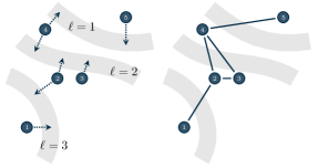
Figure 1: Network Utility Maximization problem with $5$ sources (filled circles) using $3$ links (gray stripes).

Thus, optimization problem (5) can be rewritten as

$$\begin{split}\max_{x_{1},\ldots,x_{n}}\>&\>\sum_{i=1}^{n}U_{i}(x_{i})\\ \text{subj.\ to}\>&\>\>(x_{i},\{x_{j}\}_{j\in\mathcal{N}_{i}})\in\prod_{j\in\mathcal{N}_{i}\cup\{i\}}I_{j},\>i\in\{1,\dots,n\},\\ &\sum_{j\in\mathcal{N}_{i}\cup\{i\}}\!\!a_{j,\ell}\,x_{j}\leq c_{\ell},\hskip 5.69046pt\ell\in L(i),\>i\in\{1,\dots,n\},\end{split}$$ (6)

where $\mathcal{N}_{i}$ is the neighbor set of $i$ in $\mathcal{G}$, $a_{j,\ell}$ is $1$ if agent $j$ can use link $\ell$ and $0$ otherwise. Notice that in problem (6) if sources $i$ and $j$ share a link $\ell$, then they both have the capacity constraint of link $\ell$. Moreover, in order to have compactness of the local constraint set $X_{i}$, transmission rate constraints of neighboring nodes are also taken into account. Finally, in order to fulfill the strong convexity assumption on the local costs, two strategies can be used. First, one can assume that each agent knows the utility functions of neighboring agents, so that it sets $f_{i}(x_{i},\{x_{j}\}_{j\in\mathcal{N}_{i}})=\sum_{j\in\mathcal{N}_{i}\cup\{i\}}U_{j}(x_{j})$. Alternatively, one can consider an additional separable (small) regularization term in the NUM problem formulation in (5), e.g., $\epsilon\sum_{i=1}^{n}x_{i}^{2}$ with $\epsilon>0$. In this case each agent sets its local cost function to $f_{i}(x_{i},\{x_{j}\}_{j\in\mathcal{N}_{i}})=U_{i}(x_{i})+\sum_{j\in\mathcal{N}_{i}}\epsilon_{ij}x_{j}^{2}$, where $\epsilon_{ij}>0$ are suitable fractions of $\epsilon$. Except for the maximization versus minimization, this problem is partitioned, that is it has the same structure as (2).

A problem with this structure can be also found in resource allocation problems, which are of great importance in several research areas. In the context of network systems solving resource allocation problems in a distributed way is a preliminary task to solve several control and estimation problems. Indeed, it is often the case that the agents in the network have some local resource that have to share with their neighbors.

Consider a general set-up in which each agent produces a certain amount of resource, which it can share with its neighbors (i.e., neighboring nodes in the communication graph). Each agent has a local strongly concave utility function to maximize. The resulting optimization problem turns out to be

$$\max_{x_{1},\ldots,x_{n}}\> \>\sum_{i=1}^{n}U_{i}(x_{i})$$

subj. to $$\>\sum_{j\in\mathcal{N}_{i}\cup\{i\}}x_{j}\leq r_{i},\qquad i\in\{1,\dots,n\},$$

where $x_{i}$ is the resource produced by node $i$, $r_{i}$ is the capacity of node $i$ and we are assuming that the set of neighbors with whom node $i$ can share its resource coincides with the set of neighbors in the communication graph. In other words agents can share resources only if they can communicate.

It is worth noting that dual decomposition is often used in network utility maximization and resource allocation problems. See for example [34] for a tutorial on dual decomposition methods in network utility maximization. Usually, in this context, the capacity constraints are dualized to obtain a master-subproblem or a distributed algorithm. However, in these early references, as e.g., in [33], the dual decomposition gives rise to algorithms that are not suited for a pure peer-to-peer network as the one we consider. In our partitioned approach the dual decomposition is used to enforce the coherence constraints, whereas the capacity constraints are taken into account in the primal local minimization. These aspects will be more clear in the next section in which we derive the partitioned dual decomposition approach.

III Partitioned Dual Decomposition for Distributed Optimization

In order to introduce our distributed algorithms, we derive a partitioned dual decomposition scheme by introducing suitable copies of the decision variables.

As a preliminary step, we briefly recall the standard dual decomposition approach for distributed optimization. In order to solve problem (1) in a distributed way, a common approach consists of writing it in the equivalent form

$$\begin{split}\min_{x^{(1)},\ldots,x^{(n)}}\>&\>\sum_{i=1}^{n}f_{i}(x^{(i)})\\ \text{subj.\ to}\>&\>x^{(i)}\in X_{i},\hskip 19.91684pti\in\{1,\dots,n\},\\ &\>x^{(i)}=x^{(j)},\hskip 14.22636pt(i,j)\in\mathcal{E},\end{split}$$ (7)

where each $x^{(i)}$ can be seen as a copy of $x$ subject to the additional constraint that all the copies must be equal. Clearly, the connected nature of the network ensures equality between all $x^{(i)}$ and, in turn, the equivalence between (7) and (1).

When considering a partitioned problem as in (2), because of the structure of $f_{i}$ and $X_{i}$, $i\in\{1,\dots,n\}$, the formulation (1) is considerably redundant. The idea is to exploit the partitioned structure to modify (7) in order to limit the range of equivalences among the auxiliary variables, and, in turn, their diffusion over the network.

III-A Partitioned Dual Decomposition Set-up

Once we create copies of the vector $x\in^{N}$, we enforce each state $x_{i}\in^{m_{i}}$ to be identical only for the neighboring nodes $j\in\mathcal{N}_{i}\cup\{i\}$ which use this information. Formally, we reformulate problem (2) as

$$\begin{split}\min\>&\>\sum_{i=1}^{n}f_{i}\big{(}x^{(i)}_{i},\{x^{(i)}_{j}\}_{j\in\mathcal{N}_{i}}\big{)}\\ \text{subj.\ to}\>&\>\big{(}x^{(i)}_{i},\{x^{(i)}_{j}\}_{j\in\mathcal{N}_{i}}\big{)}\in X_{i}\qquad i\in\{1,\dots,n\},\\ &\>x^{(i)}_{i}=x^{(j)}_{i},\qquad\qquad j\in\mathcal{N}_{i},\;i\in\{1,\dots,n\},\\ &\>x^{(i)}_{j}=x^{(j)}_{j},\qquad\qquad j\in\mathcal{N}_{i},\;i\in\{1,\dots,n\},\end{split}$$ (8)

where $x^{(j)}_{i}$ denotes the copy of state $x_{i}$ stored in memory of node $j$. Notice that connected nature of the graph $\mathcal{G}$ ensures equivalence between (2) and (8).

As an example, in Figure 2 we visualize the partitioned set-up for a path graph of $n=4$ nodes. Along $i$-th column, we show the coupling due to the local cost $f_{i}$ and the local constraint $X_{i}$, which involves only the states handled by node $i$, i.e., $x_{i}^{(i)}$ and $x_{j}^{(i)}$ with $j\in\mathcal{N}_{i}$. Along the $i$-th row, we show the coupling due to copies $x_{i}^{(j)}$, $j\in\mathcal{N}_{i}$, of the variable $x_{i}$.

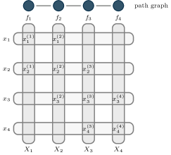
Figure 2: Partitioned optimization problem over a path graph of $n=4$ nodes.

Before proceeding with presentation of the algorithms, we discuss two key features in the structure of the above problem. First, it is worth noting that the problem formulations (7) and (8), although equivalent, are different. In fact, (8) will lead to our partitioned algorithm. Second, we point out that a constraint $x^{(i)}_{i}=x^{(j)}_{i}$ for a pair of agents $i$ and $j$ appears two times. This redundant formulation is not accidental, but plays an important role in exploiting the partitioned structure of the proposed algorithm.

Next, we introduce an aggregate notation for the copies, which allows us to be more compact in the derivation of the algorithms and their analysis. We denote by

$$y^{(i)}:=\big{(}x^{(i)}_{i},\{x^{(i)}_{j}\}_{j\in\mathcal{N}_{i}}\big{)}$$ (9)

the set of local variables of node $i$, arranged as a column vector in ${}^{\sum_{j\in\mathcal{N}_{i}\cup\{i\}}m_{j}}$. In this way we can write equivalently

$$f_{i}\big{(}x^{(i)}_{i},\{x^{(i)}_{j}\}_{j\in\mathcal{N}_{i}}\big{)}=f_{i}\big{(}y^{(i)}\big{)}\quad\text{and}\quad y^{(i)}\in X_{i}.$$

To tackle problem (8) in a distributed way, we start by deriving its dual problem. The partial Lagrangian for problem (8) is given by

$$\mathcal{L}({\mathbf{x},\Lambda}) =\sum_{i=1}^{n}\bigg{(}f_{i}\big{(}x^{(i)}_{i},\{x^{(i)}_{j}\}_{j\in\mathcal{N}_{i}}\big{)}$$ (10)

$$+\!\!\sum_{j\in\mathcal{N}_{i}}\Big{(}\lambda^{(i,j)\top}_{i}(x^{(i)}_{i}-x^{(j)}_{i})+\!\lambda^{(i,j)\top}_{j}(x^{(i)}_{j}-x^{(j)}_{j})\!\Big{)}\!\bigg{)},$$

where $\mathbf{x}$ stacks all the (primal) optimization variables in the network, while $\Lambda$ denotes the stack of dual variables, i.e.,

$$\Lambda=\big{[}\Lambda_{1}^{\top},\ldots,\Lambda_{n}^{\top}\big{]}^{\top},$$

with block $\Lambda_{i}:=[\{\lambda_{i}^{(i,j)}\}_{j\in\mathcal{N}_{i}},\{\lambda_{j}^{(i,j)}\}_{j\in\mathcal{N}_{i}}]$, $i\in\{1,\dots,n\}$.

By exploiting the undirected nature and the connectivity of graph $\mathcal{G}$, the Lagrangian (10) can be rewritten as

$$\mathcal{L}(\mathbf{x},\Lambda )=\sum_{i=1}^{n}\bigg{(}f_{i}\big{(}x^{(i)}_{i},\{x^{(i)}_{j}\}_{j\in\mathcal{N}_{i}}\big{)}$$ (11)

$$\!\!+x_{i}^{(i)\top}\!\!\sum_{j\in\mathcal{N}_{i}}(\lambda^{(i,j)}_{i}\!-\!\lambda^{(j,i)}_{i})+\!\!\sum_{j\in\mathcal{N}_{i}}x_{j}^{(i)\top}\big{(}\lambda^{(i,j)}_{j}\!-\!\lambda^{(j,i)}_{j}\big{)}\!\bigg{)}$$

which is separable with respect to $y^{(i)}$, $i\in\{1,\dots,n\}$.

Remark III.1.

It is worth noting that we have not dualized the local constraints $(x^{(i)}_{i},\{x^{(i)}_{j}\}_{j\in\mathcal{N}_{i}})\in X_{i}$ (thus the notion of partial Lagrangian) since each of them will be handled by the agents in their local optimization problem.  $\square$

The dual function of (8) is obtained by minimizing the Lagrangian with respect to the primal variables, which gives

$$\begin{split}q(\Lambda)&=\min_{\mathbf{x}\in X_{1}\times\cdots\times X_{n}}\mathcal{L}({\mathbf{x},\Lambda})\\ &=\sum_{i=1}^{n}q_{i}\Big{(}\big{\{}\lambda^{(i,j)}_{i},\lambda^{(j,i)}_{i},\lambda^{(i,j)}_{j},\lambda^{(j,i)}_{j}\big{\}}_{j\in\mathcal{N}_{i}}\Big{)}\end{split}$$

with

$$q_{i}\Big{(}\big{\{}\lambda^{(i,j)}_{i},\lambda^{(j,i)}_{i},\lambda^{(i,j)}_{j},\lambda^{(j,i)}_{j}\big{\}}_{j\in\mathcal{N}_{i}}\Big{)}=$$

$$\hskip 14.22636pt\min_{\big{(}x^{(i)}_{i},\{x^{(i)}_{j}\}_{j\in\mathcal{N}_{i}}\big{)}\in X_{i}}\!\!\Big{(}f_{i}\big{(}x^{(i)}_{i},\{x^{(i)}_{j}\}_{j\in\mathcal{N}_{i}}\big{)}$$ (12)

$$\hskip 25.6073pt+x_{i}^{(i)\top}\!\!\sum_{j\in\mathcal{N}_{i}}\!\!(\lambda^{(i,j)}_{i}\!-\!\lambda^{(j,i)}_{i})+\!\!\sum_{j\in\mathcal{N}_{i}}\!\!x_{j}^{(i)\top}(\lambda^{(i,j)}_{j}\!-\!\lambda^{(j,i)}_{j})\Big{)}.$$

Notice that, since each $X_{i}$ is compact and nonempty, the minimum in (12) is (uniquely) attained, so that $q_{i}$ is always finite. Thus, the dual problem of (8) is the following unconstrained optimization problem

$$\max_{\Lambda}\> \>\sum_{i=1}^{n}q_{i}\Big{(}\big{\{}\lambda^{(i,j)}_{i},\lambda^{(j,i)}_{i},\lambda^{(i,j)}_{j},\lambda^{(j,i)}_{j}\big{\}}_{j\in\mathcal{N}_{i}}\Big{)}.$$ (13)

Remark III.2.

Let $\varphi:^{d}\rightarrow\cup\{+\infty\}$, its conjugate function $\varphi^{*}:^{d}\rightarrow$ is defined as

$$\varphi^{*}(z):=\sup_{x}\big{(}z^{\top}x-\varphi(x)\big{)}.$$

Then,

$$q_{i}\Big{(}\big{\{}\lambda^{(i,j)}_{i},\lambda^{(j,i)}_{i},\lambda^{(i,j)}_{j},\lambda^{(j,i)}_{j}\big{\}}_{j\in\mathcal{N}_{i}}\Big{)}=$$

$$\hskip 39.83368pt-f_{i}^{*}\Big{(}\sum_{j\in\mathcal{N}_{i}}\!\!(\lambda^{(i,j)}_{i}\!-\!\lambda^{(j,i)}_{i}),\big{\{}(\lambda^{(i,j)}_{j}\!-\!\lambda^{(j,i)}_{j})\big{\}}_{j\in\mathcal{N}_{i}}\Big{)},$$

with $f_{i}^{*}$ being the conjugate function of $f_{i}$.  $\square$

Remark III.3.

It is worth noting that each $q_{i}$ does not depend on the entire set of dual variables $\Lambda$, but it exhibits a sparse structure, i.e., it is a function of the dual variables of the neighbors $\mathcal{N}_{i}$ only.  $\square$

III-B (Synchronous) Partitioned Dual Decomposition (PDD) distributed algorithm

With the dual problem in hand, a gradient algorithm on the dual problem, [35, Chapter 6], can be applied. This results into a minimization on the primal variables and a linear update on the dual variables. As we will show in the analysis, this gives rise to the PDD distributed algorithm, which is formally stated, from the perspective of node $i$, in the following table.

We point out that each node $i\in\{1,\dots,n\}$ stores and updates the primal variables $x^{(i)}_{i}$ and $x^{(i)}_{j}$, $j\in\mathcal{N}_{i}$, and the dual variables $\lambda^{(i,j)}_{i}$ and $\lambda^{(i,j)}_{j}$, $j\in\mathcal{N}_{i}$.

Processor states: $(x_{i}^{(i)},\{x_{j}^{(i)}\}_{j\in\mathcal{N}_{i}})$ and $\{\lambda_{i}^{(i,j)},\lambda_{j}^{(i,j)}\}_{j\in\mathcal{N}_{i}}$

Evolution:

 for: $t=1,2,\ldots$ do

   Compute and broadcast primal variables

$$\begin{split}&\big{(}x^{(i)}_{i}(t\!+\!1),\{x^{(i)}_{j}(t\!+\!1)\}_{j\in\mathcal{N}_{i}}\big{)}=\\ &\hskip 14.22636pt\mathop{\operatorname{argmin}}_{(x_{i},\{x_{j}\}_{j\in\mathcal{N}_{i}})\in X_{i}}\bigg{(}f_{i}\big{(}x_{i},\{x_{j}\}_{j\in\mathcal{N}_{i}}\big{)}+x_{i}^{\top}\textstyle\sum\limits_{j\in\mathcal{N}_{i}}\!\Big{(}\lambda^{(i,j)}_{i}(t)-\lambda^{(j,i)}_{i}(t)\Big{)}+\textstyle\sum\limits_{j\in\mathcal{N}_{i}}\!x_{j}^{\top}\Big{(}\lambda^{(i,j)}_{j}(t)-\lambda^{(j,i)}_{j}(t)\Big{)}\!\!\bigg{)}.\end{split}$$ (14)

   Update and broadcast dual variables via

$$\begin{split}&\lambda^{(i,j)}_{i}(t\!+\!1)=\lambda^{(i,j)}_{i}(t)\!+\!\alpha_{i}\Big{(}\!x^{(i)}_{i}(t\!+\!1)-x^{(j)}_{i}(t\!+\!1)\!\Big{)}\\ &\lambda^{(i,j)}_{j}(t\!+\!1)=\lambda^{(i,j)}_{j}(t)\!+\!\alpha_{i}\Big{(}\!x^{(i)}_{j}(t\!+\!1)-x^{(j)}_{j}(t\!+\!1)\!\Big{)}\end{split}$$ (15)

   for all $j\in\mathcal{N}_{i}$.

Distributed Algorithm 1 PDD

Before studying the convergence properties of the proposed algorithm, let us comment on its scalability and how it compares with standard dual gradients algorithms. First, observe that each node has to keep in memory the set of variables $x_{i}^{(i)}$, $\big{\{}x_{j}^{(i)}\big{\}}_{j\in\mathcal{N}_{i}}$, $\big{\{}\lambda^{(i,j)}_{i},\lambda^{(i,j)}_{j}\big{\}}_{j\in\mathcal{N}_{i}}$, namely a number of variables equal to $1+3|\mathcal{N}_{i}|$. Second, the step-sizes $\alpha_{i}$, $i\in\{1,\dots,n\}$ are constant, local and can be initialized via local computations. More details are given in Theorem III.5.

Remark III.4.

Notice that, differently from existing dual decomposition schemes, our algorithms do not enforce any symmetry in the dual variables, i.e., in general $\lambda^{(i,j)}_{i}(t)\neq-\lambda^{(j,i)}_{i}(t)$. The symmetry, although not necessary, can be imposed if the agents select a common step-size $\alpha_{i}=\alpha$, for all $i\in\{1,\dots,n\}$, and properly initialize their dual variables. As a consequence, the algorithm can be simplified to have only one communication round to perform both the local minimization and the ascent. $\square$

The convergence properties of PDD (Distributed Algorithm 1) are established in the following theorem.

Theorem III.5.

Let Assumptions II.1, II.2 and II.3 hold true and assume the step-sizes $\alpha_{i}$, $i\in\{1,\dots,n\}$, to be constant and such that $0<\alpha_{i}\leq\frac{1}{nL_{i}}$, with

$$L_{i}=\sqrt{2\textstyle\sum\limits_{j\in\mathcal{N}_{i}}\Big{(}\frac{1}{\sigma_{i}}+\frac{1}{\sigma_{j}}\Big{)}^{2}},\quad\forall\,i\in\{1,\dots,n\}.$$ (16)

Then, the sequence $\{\Lambda_{1}(t),\ldots,\Lambda_{n}(t)\}$ generated by PDD (Distributed Algorithm 1) converges in objective value to the optimal cost $f^{\star}$ of problem (2). Moreover, let $x^{\star}=(x_{1}^{\star\top},\ldots,x_{n}^{\star\top})^{\top}$ be the unique optimal solution of (2), then each primal sequence $x_{i}^{(i)}(t)$ generated by PDD is such that

$$\lim_{t\to\infty}\,\|x_{i}^{(k)}(t)-x_{i}^{\star}\|=0,$$

for all $i\in\{1,\dots,n\}$ and $k\in\{i\}\cup\mathcal{N}_{i}$.

Proof.

We structure the proof of the first statement in three parts in which we show that: (i) the dual gradient has a block structure and smoothness, (ii) the distributed algorithm implements a diagonally-scaled gradient method, and (iii) strong duality holds. First, consider the dual problem (13) and a block partitioning of dual variables $\Lambda=[\Lambda_{1},\ldots,\Lambda_{n}]$, with

$$\Lambda_{i}:=\Big{(}\{\lambda_{i}^{(i,j)}\}_{j\in\mathcal{N}_{i}},\{\lambda_{j}^{(i,j)}{j\in\mathcal{N}_{i}}\}\Big{)}$$ (17)

representing the local variables of node $i$, for all $i\in\{1,\dots,n\}$. Under Assumption II.1, the dual function $q(\Lambda)$ is guaranteed to have block-coordinate Lipschitz continuous gradient $\nabla q(\Lambda)$ with block constants $L_{i}$, $i\in\{1,\dots,n\}$, given in (16). In fact, we can explicitly compute the components of $\nabla q(\Lambda)$ associated to each block $\Lambda_{i}$, denoted hereafter as $\nabla_{\Lambda_{i}}q(\Lambda)$, by using the chain rule of derivation and the conjugate function notation. We have that

$$\begin{split}\frac{\partial q(\Lambda)}{\partial\lambda_{i}^{(i,j)}}&=(\nabla f_{i}^{*})_{i}-(\nabla f_{j}^{*})_{i},\>j\in\mathcal{N}_{i}\\ \frac{\partial q(\Lambda)}{\partial\lambda_{j}^{(i,j)}}&=(\nabla f_{i}^{*})_{j}-(\nabla f_{j}^{*})_{j},\>j\in\mathcal{N}_{i},\end{split}$$ (18)

where $(\nabla f_{i}^{*})_{i}$ denotes the $i$-th component of $\nabla f_{i}^{*}$ and we omit the argument of $\nabla f_{i}^{*}$ to take light the notation. Since for all $i\in\{1,\dots,n\}$, each $f_{i}$ is a strongly convex function, then the gradient of its conjugate function $\nabla f_{i}^{*}$ is Lipschitz continuous with constant $1/\sigma_{i}$, [36, Chapter X, Theorem 4.2.2]. By considering the Euclidean $2$-norm, in light of (18) and by simple algebraic manipulation, we can conclude that also $\nabla_{\Lambda_{i}}q(\Lambda)$ is Lipschitz continuous with constant

$$L_{i}=\sqrt{\textstyle\sum\limits_{j\in\mathcal{N}_{i}}\Big{(}\frac{1}{\sigma_{i}}+\frac{1}{\sigma_{j}}\Big{)}^{2}+\textstyle\sum\limits_{j\in\mathcal{N}_{i}}\Big{(}\frac{1}{\sigma_{i}}+\frac{1}{\sigma_{j}}\Big{)}^{2}},$$

which matches (16). Second, we show that our PDD distributed algorithm implements a scaled gradient ascent method to solve problem (13). Consider a diagonal positive definite matrix defined as $W:=\operatorname{diag}(\alpha_{1},\ldots,\alpha_{n})\preceq\operatorname{diag}(\frac{1}{nL_{1}},\ldots,\frac{1}{nL_{n}})$. Formally, the scaled gradient ascent method can be written as

$$\Lambda(t+1)=\Lambda(t)+W\nabla q(\Lambda(t)),$$ (19)

where $t$ denotes the iteration counter. Since each entry of the scaling matrix satisfies $0<\alpha_{i}\leq\frac{1}{nL_{i}}$ for all $i\in\{1,\dots,n\}$, then the following condition holds [17, Theorem 8]

$$q(\Lambda(t)+\delta)\geq q(\Lambda(t))+\nabla q(\Lambda(t))^{\!\top}\delta-\frac{n}{2}\delta^{\!\top\!}\!\begin{bmatrix}L_{1}\\[-5.69046pt] &\ddots\\[-1.42271pt] &&L_{n}\end{bmatrix}\!\delta,$$

for every perturbation $\delta$. Thus, using the same line of proof of the gradient algorithm [35, Chapter 2], we can conclude that the sequence $\{\Lambda(t)\}$ generated by iteration (19) converges in objective value to the optimal cost $q^{\star}$ of (13). Since $W$ is diagonal, then (19) splits in a component-wise fashion giving

$$\Lambda_{i}(t+1)=\Lambda_{i}(t)+W_{ii}\nabla_{\Lambda_{i}}q(\Lambda(t)),\>i\in\{1,\dots,n\},$$ (20)

where $W_{ii}$ denotes the $(i,i)$-th entry of $W$. By using the following property of conjugate functions

$$\nabla\varphi^{*}(z)=\mathop{\operatorname{argmin}}_{x}\big{(}\varphi(x)-z^{\top}x\big{)},$$

we have that the primal minimization (14) computes $\nabla f_{i}^{*}$ evaluated at the point $\big{(}\sum_{j\in\mathcal{N}_{i}}(\lambda^{(i,j)}_{i}(t)-\lambda^{(j,i)}_{i}(t)),\{(\lambda^{(i,j)}_{j}(t)-\lambda^{(j,i)}_{j}(t))\}_{j\in\mathcal{N}_{i}}\big{)}$. Then

$$\begin{split}\frac{\partial q(\Lambda(t))}{\partial\lambda_{i}^{(i,j)}}&=x_{i}^{(i)}(t+1)-x_{i}^{(j)}(t+1),\>j\in\mathcal{N}_{i}\\ \frac{\partial q(\Lambda(t))}{\partial\lambda_{j}^{(i,j)}}&=x_{j}^{(i)}(t+1)-x_{j}^{(j)}(t+1),\>j\in\mathcal{N}_{i},\end{split}$$ (21)

so that update (15) is the scaled gradient ascent (20). Third and final, by Assumption II.3 (Slater’s condition), strong duality between problems (8) and (13) holds. Moreover, since problems (8) and (2) are equivalent, then they both have optimal cost $q^{\star}=f^{\star}$. Thus, the sequence $\{\Lambda(t)\}$ generated by PDD converges in objective value to the optimal cost $f^{\star}$ of (2).

For the second part of the statement, we first notice that in light of Assumptions II.1 and II.2, problem (2) has a unique optimal solution $x^{\star}=(x_{1}^{\star\top},\ldots,x_{n}^{\star\top})^{\top}$. Further, since problem (8) is equivalent to problem (2), then $x^{\star}$ is the unique optimal solution also for problem (8). Finally, the first order optimality condition for the (unconstrained) dual problem (13) is $\nabla q(\Lambda^{\star})=0$, where $\Lambda^{\star}$ is a limit point of the sequence $\{\Lambda(t)\}$ (which exists by the Lipschitz continuity of $\nabla q(\Lambda)$). This allows us to conclude, by equation (21), that the limit point of the primal sequences $\{x_{i}^{(i)}(t),\{x_{j}^{(i)}\}_{j\in\mathcal{N}_{i}}(t)\}$ satisfy the primal coherence constraints. Thus, in the limit the copies $x_{i}^{(i)},\{x_{i}^{(j)}\}_{j\in\mathcal{N}_{i}}$ of the variable $x_{i}$ are equal to the (unique) optimal $x_{i}^{\star}$. Iterating on $i\in\{1,\dots,n\}$ the proof follows. ∎

Remark III.6.

Alternative expressions for $L_{i}$ in (16) can be used. Larger upper bounds on the step-sizes $\alpha_{i}$ can be established by exploiting tailored descent conditions. See, e.g., works [14, 17, 26].  $\square$

III-C Asynchronous Partitioned Dual Decomposition (AsynPDD) distributed algorithm

In this section we present an asynchronous partitioned distributed algorithm, and prove its convergence with high probability. This algorithm can be interpreted as an extension of the PDD distributed algorithm.

We consider an asynchronous protocol where each node has its own concept of time defined by a local timer, which randomly and independently of the other nodes triggers when to awake itself. Each node is in an idle mode, wherein it continuously receives messages from neighboring nodes, until it is triggered either by the local timer or by a message from neighboring nodes. When a trigger occurs, it switches into an awake mode in which it updates its local variables and possibly transmits the updated information to its neighbors. The timer is modeled by means of a local clock $\tau_{i}\in_{\geq 0}$ and a randomly generated waiting time $T_{i}$. The timer triggers the node when $\tau_{i}=T_{i}$, so that the node switches to the awake mode and, after running the local computation, resets $\tau_{i}=0$ and extracts a new realization of $T_{i}$. We make the following assumption on the local waiting times $T_{i}$.

Assumption III.7 (Exponential i.i.d. local timers).

The waiting times between consecutive triggering events are i.i.d. random variables with same exponential distribution.  $\square$

Informally, the asynchronous distributed optimization algorithm is as follows. When a node $i$ is in idle, it continuously receives messages from awake neighbors. If the local timer $\tau_{i}$ triggers or new dual variables $\lambda_{i}^{(j,i)}$, $\lambda_{j}^{(j,i)}$ are received, it wakes up. When node $i$ wakes up, it updates and broadcasts its primal variable $y^{(i)}=\big{(}x_{i}^{(i)},\{x_{j}^{(i)}\}_{j\in\mathcal{N}_{i}}\big{)}$, computed through a local constrained minimization. Moreover, if the transition was due to the local timer triggering, then it also updates and broadcasts its local dual variables $\lambda_{i}^{(i,j)}$ and $\lambda_{j}^{(i,j)}$, $j\in\mathcal{N}_{i}$. Since there is no global iteration counter, we highlight the difference between updated and not updated values during the “awake” phase, by means of a “⁺” superscript symbol, e.g., we denote the updated primal variable as $x_{i}^{(i)+}$.

We want to stress some important aspects of the idle/awake cycle. First, these two phases are regulated by local timers and local information exchange, without the need of any central clock. Second, we assume that the computation in idle takes a negligible time compared to the one performed in the awake phase. Moreover, a constant, local step-size $\alpha_{i}$ is used in the ascent step, which can be initialized by means of local exchange of information between neighboring nodes. Finally, we point out that each agent uses the most updated values that are locally available to perform every computation.

The AsynPDD distributed algorithm is formally described in the following table.

Processor states: $(x_{i}^{(i)},\{x_{j}^{(i)}\}_{j\in\mathcal{N}_{i}})$ and $\{\lambda_{i}^{(i,j)},\lambda_{j}^{(i,j)}\}_{j\in\mathcal{N}_{i}}$

   Set $\tau_{i}=0$ and get a realization $T_{i}$

Evolution:

IDLE:

  while: $\tau_{i}<T_{i}$ do:

    Receive $\lambda_{i}^{(j,i)}$, $\lambda_{j}^{(j,i)}$ and/or $x_{i}^{(j)}$, $x_{j}^{(j)}$ from $j\in\mathcal{N}_{i}$.

    if:​ dual variables are received go to AWAKE.

   go to AWAKE.

AWAKE:

   Compute and broadcast

$$\big{(}x^{(i)+}_{i},\{x^{(i)+}_{j}\}_{j\in\mathcal{N}_{i}}\big{)}=\mathop{\operatorname{argmin}}_{(x_{i},\{x_{j}\}_{j\in\mathcal{N}_{i}})\in X_{i}}\!f_{i}(x_{i},\{x_{j}\}_{j\in\mathcal{N}_{i}})+x_{i}^{\top}\sum_{j\in\mathcal{N}_{i}}\big{(}\lambda_{i}^{(i,j)}-\lambda_{i}^{(j,i)}\big{)}+\sum_{j\in\mathcal{N}_{i}}x_{j}^{\top}\big{(}\lambda_{j}^{(i,j)}-\lambda_{j}^{(j,i)}\big{)}$$

   if:​ $\tau_{i}=T_{i}$ then:​ update and broadcast

$$\begin{split}\lambda_{i}^{(i,j)+}&=\lambda_{i}^{(i,j)}+\alpha_{i}\big{(}x_{i}^{(i)+}-x_{i}^{(j)}\big{)},\>\>\forall\,j\in\mathcal{N}_{i},\\ \lambda_{j}^{(i,j)+}&=\lambda_{j}^{(i,j)}+\alpha_{i}\big{(}x_{j}^{(i)+}-x_{j}^{(j)}\big{)},\>\>\forall\,j\in\mathcal{N}_{i},\end{split}$$ (22)

     set $\tau_{i}=0$ and get a new realization $T_{i}$.

   Go to IDLE.

Distributed Algorithm 2 AsynPDD

It is worth pointing out that being the algorithm asynchronous, for the analysis we need to carefully formalize the concept of algorithm iterations. We will use a nonnegative integer variable $t$ indexing a change in the whole state $\Lambda=[\Lambda_{1}\ldots\Lambda_{n}]$ of the distributed algorithm. In particular, each triggering will induce an iteration of the distributed optimization algorithm and will be indexed with $t$. We want to stress that this (integer) variable $t$ does not need to be known by the agents. That is, this timer is not a common clock and is only introduced for the sake of analysis.

Theorem III.8.

Let Assumptions II.1, II.2 and II.3 hold true. Let the timers $\tau_{i}$ satisfy Assumption III.7 and step-sizes $\alpha_{i}$ be constant and such that $0<\alpha_{i}\leq 1/L_{i}$, with

$$L_{i}=\sqrt{2\textstyle\sum\limits_{j\in\mathcal{N}_{i}}\Big{(}\frac{1}{\sigma_{i}}+\frac{1}{\sigma_{j}}\Big{)}^{2}},\quad\forall\,i\in\{1,\dots,n\}.$$ (23)

Then, the random sequence $\{\Lambda_{1}(t),\ldots,\Lambda_{n}(t)\}$ generated by the AsynPDD (Distributed Algorithm 2), converges with high probability in objective value to the optimal cost $f^{\star}$ of problem (2), i.e., for any $\varepsilon\in(0,q_{0})$, with $q_{0}:=q(\Lambda(0))$, and target confidence $0<\rho<1$, there exists $\bar{t}(\varepsilon,\rho)$ such that for all $t\geq\bar{t}(\varepsilon,\rho)$ it holds: $\Pr\Big{(}\big{|}q(\Lambda(t))-f^{\star}\big{|}\leq\varepsilon\Big{)}\geq 1-\rho.$

Proof.

Our proof strategy is based on showing that the iterations of the asynchronous distributed algorithm can be written as the iterations of an ad-hoc version of the coordinate method [16], applied to the dual problem (13).

Let the optimization variable $\Lambda$ be partitioned in $n$ blocks $[\Lambda_{1},\ldots,\Lambda_{n}]$ as in (17), then a coordinate approach consists in an iterative scheme in which only a block-per-iteration, say $\Lambda_{i_{t}}$ at time $t$, of the entire optimization variable $\Lambda$ is updated at time $t$, while all the other components $\Lambda_{j}$ with $j\in\{1,\dots,n\}\setminus\{i_{t}\}$ stay unchanged. Formally, a coordinate iteration can be summarized as

$$\begin{split}\Lambda_{i_{t}}(t+1)&=\Lambda_{i_{t}}(t)+\nabla_{\Lambda_{i_{t}}}q(\Lambda(t))\\ \Lambda_{j}(t+1)&=\Lambda_{j}(t),\hskip 68.28644ptj\neq i_{t}.\end{split}$$ (24)

In the following, we show that the AsynPDD distributed algorithm implements (24) with a uniform random selection of the blocks. Since the timers $\tau_{i}$ trigger independently according to the same exponential distribution, then from an external, global perspective, the induced awaking process of the nodes corresponds to the following: only one node per iteration, say $i_{t}$, wakes up randomly, uniformly and independently from previous iterations. Thus, each triggering, which induces an iteration of the distributed optimization algorithm and is indexed with $t$, corresponds to the (uniform) selection of a node in $\{1,\dots,n\}$ that becomes awake.

Next we show by induction that if each node $i$ has an updated version of the neighboring variables before it gets awake, then the same holds after the update. When node $i$ wakes up, it uses for its update its own primal variables $x_{i}^{(i)}$ and $x_{j}^{(i)}$, $j\in\mathcal{N}_{i}$, which are clearly updated since $i$ is the one modifying them. Moreover, node $i$ uses also $x_{i}^{(j)}$ and $x_{j}^{(j)}$, $j\in\mathcal{N}_{i}$, which are received by neighboring nodes $j\in\mathcal{N}_{i}$. These variables are updated by $j$ if itself or one of its neighbors becomes awake. In both cases node $j$ sends the updated variable to its neighbors (which include node $i$). An analogous argument holds for the dual variables.

Thanks to the argument just shown and by noticing that $\lambda_{i_{t}}^{({i_{t}},j)}$ and $\lambda_{j}^{({i_{t}},j)}$, $j\in\mathcal{N}_{i_{t}}$ are the components of $\Lambda_{i_{t}}$, we have that step (22) corresponds to step (24) with $i_{t}$ randomly uniformly distributed over $\{1,\dots,n\}$. Finally, recalling that (i) the cost function $q(\Lambda)$ of problem (13) has block-coordinate Lipschitz continuous gradient with respect to the blocks $\Lambda_{i}$ (see proof of Theorem III.5) and (ii) the step-sizes $\alpha_{i}$ are constant and such that $0<\alpha_{i}\leq 1/L_{i}$ with $L_{i}$ in (23), we can invoke [16, Theorem 5] to conclude that the coordinate method (24) (and equivalently the AsynPDD distributed algorithm) converges with high probability to the optimal cost $q^{\star}$ of problem (13). Recalling that strong duality between problems (2) and (13) holds (see proof of Theorem III.5), then $q^{\star}=f^{\star}$, and the proof follows. ∎

Remark III.9.

As highlighted in Theorem III.8 in order to set the local step-sizes $\alpha_{i}$, each node $i$ should know the convexity parameter $\sigma_{j}$ of its neighbors but, differently from the synchronous case (cf. condition (16)), does not need to know the total number of agents $n$ in the network.  $\square$

To conclude this section, we notice that the asynchronous model employed in our distributed algorithm can be generalized. In fact, in the considered model timers are drawn from a common exponential distribution, while independent and completely uncoordinated rules might be more desiderable. This generalization is currently under investigation.

IV Numerical Simulations

In this section we provide a numerical example showing the effectiveness of the proposed techniques. We test the proposed distributed algorithms on a quadratic program enjoying the partitioned structure described in the previous sections. Specifically, we consider a network of $n=100$ agents communicating according to an undirected connected Erdős-Rényi random graph $\mathcal{G}$ with parameter $p=0.2$. Thus, letting $\big{(}x_{i},\big{\{}x_{j}\big{\}}_{j\in\mathcal{N}_{i}}\big{)}$ denote a column vector, we consider the following partitioned optimization problem

$$\begin{split}\min_{x}\>&\>\sum_{i=1}^{n}\big{(}x_{i},\big{\{}x_{j}\big{\}}_{j\in\mathcal{N}_{i}}\big{)}^{\top}Q_{i}\big{(}x_{i},\big{\{}x_{j}\big{\}}_{j\in\mathcal{N}_{i}}\big{)}+r_{i}^{\top}\!\big{(}x_{i},\big{\{}x_{j}\big{\}}_{j\in\mathcal{N}_{i}}\big{)}\\[4.64996pt] \text{subj.\ to}\>&\>A_{i}\big{(}x_{i},\big{\{}x_{j}\big{\}}_{j\in\mathcal{N}_{i}}\big{)}\preceq b_{i},\hskip 14.22636pti\in\{1,\dots,n\},\end{split}$$ (25)

where each $x_{i}\in^{m_{i}}$ and $m_{i}$ is uniformly drawn from $\{1,2,3,4\}$. This optimization problem has the same partitioned structure discussed in Section III-A. In particular, we have quadratic cost functions $f_{i}(x_{i},\{x_{j}\}_{j\in\mathcal{N}_{i}})$ and linear constraints $X_{i}=\{(x_{i},\big{\{}x_{j}\big{\}}_{j\in\mathcal{N}_{i}})\mid A_{i}(x_{i},\big{\{}x_{j}\big{\}}_{j\in\mathcal{N}_{i}})\preceq b_{i}\}$. The matrices $Q_{i}$ are positive definite with eigenvalues uniformly generated in $[1,20]$, while the vectors $r_{i}$ have entries randomly generated in $[0,100]$. Moreover, each pair $A_{i}$, $b_{i}$ describes a linear constraint having a number of rows uniformly drawn from $\{1,2\}$. Each $A_{i}$ has entries normally distributed with zero mean and unitary variance, while $b_{i}$ are suitably generated to always obtain feasible linear constraints. For all $i\in\{1,\dots,n\}$, we use constant step-sizes $\alpha_{i}=L_{i}$ with $L_{i}$ computed as in (16) for the synchronous algorithm and as in (23) for the asynchronous case. All the dual variables are initialized to zero.

In Figure 3 we show the convergence rate of the synchronous distributed algorithm by plotting the difference between the dual cost $q(\Lambda(t))$ at each iteration $t$ and the optimal value $q^{\star}=f^{\star}$ of problem (25).

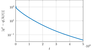
Figure 3: Evolution of the cost error for the synchronous distributed algorithm.

In Figure 4 we show the evolution of the difference between the generated primal sequence $\{x_{1}^{(1)}(t),\ldots,x_{n}^{(n)}(t)\}$ and the (unique) optimal primal solution $x^{\star}$.

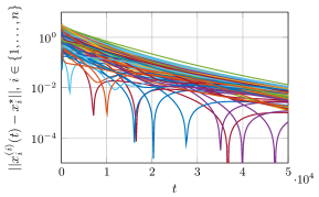
Figure 4: Evolution of the error on primal variables $x_{i}^{(i)}$, $i\in\{1,\dots,n\}$, for the synchronous distributed algorithm.

In Figure 5 we show the disagreement on the primal variable $x_{2}$ between neighboring nodes $\mathcal{N}_{2}\cup\{2\}$. In particular, we plot the norm of $x_{2}^{(2)}(t)-x_{2}^{(j)}(t)$, for all $j\in\mathcal{N}_{2}\cup\{2\}$.

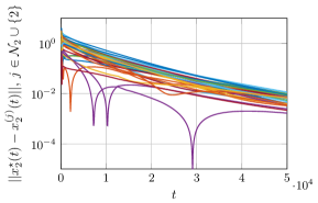
Figure 5: Evolution of the disagreement on $x_{2}$ between agents $2$ and its neighbors $j\in\mathcal{N}_{2}$ for the synchronous distributed algorithm.

Finally, in Figure 6 we show the convergence rate for the AsynPDD distributed algorithm. Since we are dealing with an asynchronous algorithm, we normalize the iteration counter $t$ with respect to the total number of agents $n$. It is worth noting the cost evolution is not monotone as expected for the class of randomized algorithms.

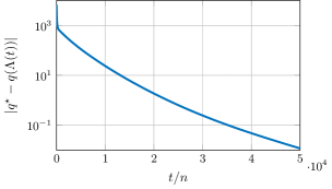
Figure 6: Evolution of the cost error for the asynchronous distributed algorithm.

V Conclusions

In this paper we have proposed a synchronous and an asynchronous distributed optimization algorithms, based on dual decomposition, for a novel partitioned distributed optimization framework. In this framework each node in the network is assigned a local state, objective function and constraint. The objective function and the constraints only depend on the node state and on its neighbors’ states. This scenario includes several interesting problems as network utility maximization and resource allocation, static state estimation in power networks, localization in wireless networks, and map building in robotic networks. The proposed algorithms are distributed and scalable and are shown to be convergent under standard assumptions on the cost functions and on the constraints sets.

References

- [1] R. Carli and G. Notarstefano, “Distributed partition-based optimization via dual decomposition,” in IEEE 52nd Conference on Decision and Control (CDC), 2013, pp. 2979–2984.
- [2] A. Nedić and A. Ozdaglar, “Distributed subgradient methods for multi-agent optimization,” IEEE Transactions on Automatic Control, vol. 54, no. 1, pp. 48–61, 2009.
- [3] A. Nedić, A. Ozdaglar, and P. A. Parrilo, “Constrained consensus and optimization in multi-agent networks,” IEEE Transactions on Automatic Control, vol. 55, no. 4, pp. 922–938, 2010.
- [4] B. Yang and M. Johansson, “Distributed optimization and games: A tutorial overview,” Networked Control Systems, pp. 109–148, 2011.
- [5] H. Terelius, U. Topcu, and R. M. Murray, “Decentralized multi-agent optimization via dual decomposition,” IFAC Proceedings Volumes, vol. 44, no. 1, pp. 11 245–11 251, 2011.
- [6] M. Zhu and S. Martínez, “On distributed convex optimization under inequality and equality constraints,” IEEE Transactions on Automatic Control, vol. 57, no. 1, pp. 151–164, 2012.
- [7] J. C. Duchi, A. Agarwal, and M. J. Wainwright, “Dual averaging for distributed optimization: convergence analysis and network scaling,” IEEE Transactions on Automatic Control, vol. 57, no. 3, pp. 592–606, 2012.
- [8] A. Falsone, K. Margellos, S. Garatti, and M. Prandini, “Dual decomposition for multi-agent distributed optimization with coupling constraints,” Automatica, vol. 84, pp. 149–158, 2017.
- [9] I. D. Schizas, A. Ribeiro, and G. B. Giannakis, “Consensus in ad hoc WSNs with noisy links – part I: Distributed estimation of deterministic signals,” IEEE Transactions on Signal Processing, vol. 56, no. 1, pp. 350 – 364, 2008.
- [10] T.-H. Chang, M. Hong, and X. Wang, “Multi-agent distributed optimization via inexact consensus ADMM,” IEEE Transactions on Signal Processing, vol. 63, no. 2, pp. 482–497, 2015.
- [11] E. Wei and A. Ozdaglar, “On the convergence of asynchronous distributed alternating direction method of multipliers,” in IEEE Global Conference on Signal and Information Processing, 2013, pp. 551–554.
- [12] M. Bürger, G. Notarstefano, and F. Allgöwer, “A polyhedral approximation framework for convex and robust distributed optimization,” IEEE Transactions on Automatic Control, vol. 59, no. 2, pp. 384–395, 2014.
- [13] D. P. Bertsekas and J. N. Tsitsiklis, Parallel and distributed computation: numerical methods. Prentice-Hall, Inc., 1989.
- [14] Y. Nesterov, “Efficiency of coordinate descent methods on huge-scale optimization problems,” SIAM Journal on Optimization, vol. 22, no. 2, pp. 341–362, 2012.
- [15] ——, “Gradient methods for minimizing composite functions,” Mathematical Programming, vol. 140, no. 1, pp. 125–161, 2013.
- [16] P. Richtárik and M. Takáč, “Iteration complexity of randomized block-coordinate descent methods for minimizing a composite function,” Mathematical Programming, vol. 144, no. 1-2, pp. 1–38, 2014.
- [17] ——, “Parallel coordinate descent methods for big data optimization,” Mathematical Programming, vol. 156, no. 1-2, pp. 433–484, 2016.
- [18] F. Facchinei, G. Scutari, and S. Sagratella, “Parallel selective algorithms for nonconvex big data optimization,” IEEE Transactions on Signal Processing, vol. 63, no. 7, pp. 1874–1889, 2015.
- [19] A. Daneshmand, F. Facchinei, V. Kungurtsev, and G. Scutari, “Hybrid random/deterministic parallel algorithms for nonconvex big data optimization,” IEEE Transactions on Signal Processing, vol. 63, no. 15, pp. 3914–3929, 2015.
- [20] A. Patrascu and I. Necoara, “Efficient random coordinate descent algorithms for large-scale structured nonconvex optimization,” Journal of Global Optimization, vol. 61, no. 1, pp. 19–46, 2015.
- [21] I. Necoara, “Random coordinate descent algorithms for multi-agent convex optimization over networks,” IEEE Transactions on Automatic Control, vol. 58, no. 8, pp. 2001–2012, 2013.
- [22] P. Bianchi, W. Hachem, and F. Iutzeler, “A coordinate descent primal-dual algorithm and application to distributed asynchronous optimization,” IEEE Transactions on Automatic Control, vol. 61, no. 10, pp. 2947–2957, 2016.
- [23] I. Notarnicola and G. Notarstefano, “Asynchronous distributed optimization via randomized dual proximal gradient,” IEEE Transactions on Automatic Control, vol. 62, no. 5, pp. 2095–2106, 2017.
- [24] T. Erseghe, “A distributed and scalable processing method based upon ADMM,” IEEE Signal Processing Letters, vol. 19, no. 9, pp. 563–566, 2012.
- [25] ——, “A distributed and maximum-likelihood sensor network localization algorithm based upon a nonconvex problem formulation,” IEEE Transactions on Signal and Information Processing over Networks, vol. 1, no. 4, pp. 247–258, 2015.
- [26] I. Necoara and D. Clipici, “Parallel random coordinate descent method for composite minimization: Convergence analysis and error bounds,” SIAM Journal on Optimization, vol. 26, no. 1, pp. 197–226, 2016.
- [27] M. Todescato, G. Cavraro, R. Carli, and L. Schenato, “A robust block-Jacobi algorithm for quadratic programming under lossy communications,” IFAC-PapersOnLine, vol. 48, no. 22, pp. 126–131, 2015.
- [28] J. F. Mota, J. M. Xavier, P. M. Aguiar, and M. Püschel, “Distributed optimization with local domains: Applications in MPC and network flows,” IEEE Transactions on Automatic Control, vol. 60, no. 7, pp. 2004–2009, 2015.
- [29] ——, “D-ADMM: A communication-efficient distributed algorithm for separable optimization,” IEEE Transactions on Signal Processing, vol. 61, no. 10, pp. 2718–2723, 2013.
- [30] F. Pasqualetti, R. Carli, and F. Bullo, “Distributed estimation via iterative projections with application to power network monitoring,” Automatica, vol. 48, no. 5, pp. 747–758, 2012.
- [31] F. C. Schweppe and J. Wildes, “Power system static-state estimation, part II: Approximate model.” IEEE Transactions on Power Apparatus and Systems, vol. 89, no. 1, pp. 125–130, 1970.
- [32] F. P. Kelly, A. K. Maulloo, and D. K. Tan, “Rate control for communication networks: shadow prices, proportional fairness and stability,” Journal of the Operational Research, vol. 49, no. 3, pp. 237–252, 1998.
- [33] S. H. Low and D. E. Lapsley, “Optimization flow control, I: basic algorithm and convergence,” IEEE/ACM Transactions on Networking, vol. 7, no. 6, pp. 861–874, 1999.
- [34] D. P. Palomar and M. Chiang, “A tutorial on decomposition methods for network utility maximization,” IEEE Journal on Selected Areas in Communications, vol. 24, no. 8, pp. 1439–1451, 2006.
- [35] D. P. Bertsekas, Nonlinear programming. Athena scientific, 1999.
- [36] J.-B. Hiriart-Urruty and C. Lemaréchal, “Convex analysis and minimization algorithms II: Advanced theory and bundle methods,” Grundlehren der mathematischen Wissenschaften, vol. 306, 1993.