Rule-Based Drawing, Analysis and Generation of Graphs for Mason’s Mark Design
Tool Description

Abstract

We are developing a rule-based implementation of a tool to analyse and generate graphs. It is currently used in the domain of mason’s marks. For thousands of years, stonemasons have been inscribing these symbolic signs on dressed stone. Geometrically, mason’s marks are line drawings. They consist of a pattern of straight lines, sometimes circles and arcs. We represent mason’s marks by connected planar graphs.

Our prototype tool for analysis and generation of graphs is written in the rule-based declarative language Constraint Handling Rules. It features

• a vertex-centric logical graph representation as constraints,

• derivation of properties and statistics from graphs,

• recognition of (sub)graphs and patterns in a graph,

• automatic generation of graphs from given constrained subgraphs,

• drawing graphs by visualization using svg graphics

In particular, we started to use the tool to classify and to invent mason’s marks. In principe, our tool can be applied to any problem domain that admits a modeling as graphs.

1 Introduction

Mason’s marks are symbols often found on dressed stone in historic buildings. These signs go back about 4500 years, to the tombs of the advanced ancient civilization of Egypt. In Europe, they were common from the 12th century on [Fri32, Dav54]. There, one can mainly find mason’s marks from the medieval ages, mostly in churches, cathedrals and monasteries. In one such building, there may be a thousand mason’s marks of hundred different designs. Over time, mason’s marks got smaller and more complex.

These mason’s marks were inscribed on the stones by stonemasons during construction of a building to identify their work, presumably for quality control and probably to receive payment. This was important for masons who were free of servitude and therefore allowed to travel the country for work (see [Fol10] for popular fiction on the subject). Only certain stonemason masters were allowed to inscribe their mark in a blazon, like a signature. Their mason’s marks are also found on medieval documents and masons tombstones. The master would give a personal mason’s mark to his apprentices, provided they had enough skill to construct and interpret the mason’s mark symbol. A challenging design and interpretation would make it harder to appropriate or misuse a mason’s mark. Stonemason’s mark are an important source of information for art and architecture historians and archaeologists, in particular to reconstruct the construction process of buildings.

Mason’s marks tend to be simple geometric symbols, usually constructed using rulers and compasses and precisely cut with a chisel. In this way a distinctive sign consisting of straight lines and curves could be produced with little effort. The geometric construction of mason’s marks implies that they exhibit a structural regularity. This was first discussed and formalized by Franz von Ržiha [Rži81]. He claimed that mason’s marks are small subfigures of regular grids, which consist either of squares or equilateral triangles together with circles inscribed in each other. His theory is obsolete, because there is no historical evidence that grids were explicitly used and because not all marks fit these grid patterns. It is however clear that the construction of the mason’s marks with compasses and rulers lends itself to the prevalence of certain angles (multiples of $30$ and $45$ degrees) between lines and certain multiples of line lengths ($1,\sqrt{2},\sqrt{3},2,\sqrt{5}\ldots$).

We are developing a graph tool and apply it to draw, analyse and generate mason’s mark designs. In this paper, we shortly present the representation of straight-line graphs, how for analysis we produce statistics about graph properties, and how we recognize subgraphs using pattern matching rules. Then we introduce our node-centric representation of line graphs and describe how to exhaustively or randomly generate graphs from given small constrained subgraphs. We conclude by discussing related and future work.

2 Tool Description

Our prototype graph analysis and generation tool is currently implemented using CHR in SWI Prolog [WDKTF14]. We assume some basic familiarity with Prolog and Constraint Handling Rules (CHR) [Frü15, Frü09]. Constraints are special relations, predicates of first order logic. They are defined by CHR rules, consisting of a left-hand-side, a guard and a right-hand-side. When the constraint pattern on the left-hand-side matches some of the current constraints and the guard test (precondition) succeeds under this matching, the right hand side of the rule is executed. Depending on the rule type, matched constraints may be removed or not. The right hand side will typically compute and add new constraints.

2.1 Representation of Mason Marks as Graphs

We represent mason’s marks (without arcs) by connected planar straight-line graphs, a drawing of planar graphs in the plane such that its edges are straight line segments [Tam13]. A line (segment) has two nodes, or endpoints, given by Cartesian coordinates. Each point is defined by a pair of numbers written X-Y. For convenience of manipulation, we redundantly represent lines at the same time by polar coordinates, which consist of a reference point (pole), which is the first endpoint of the line, a line length (radius) and an angle (azimuth) in degrees. This leads to the line constraint:

 l(EndPoint1, EndPoint2, LineLength, Angle)

With polar coordinations, translation, rotation and scaling of lines is straightforward. Only when the lines are drawn, missing point coordinates are computed:

l(X1-Y1,P2,L,A) ==> numbers(X1,X2,L,A) |
           X2 is X1+L*U*cos(A*pi/180), Y2 is Y1+L*U*sin(A*pi/180),
           P2=(X2-Y2).
 % analogously for point P1 when P2 is known

This propagation rule of the form LeftSide ==> Guard | RightSide can be read as follows: If a line matching l(X1-Y1,P2,L,A) is found where X1,X2,L,A are numbers (instead of yet unbound variables), then compute X2 and Y2 using Prolog’s is built-in and equate (unify) the endpoint P2 with the coordinate X2-Y2 using Prolog’s = built-in. If P2 was a free (unbound) variable, it will be bound, otherwise a equality check will be performed.

2.2 Analysis of Graphs

From a given graph, i.e. its line constraints, we can generate information using propagation rules. For example, one can compute counts for the occurrences of each value in the components of a line (points, lengths, angles) to collect statistical information about the graph. Note that the number of occurrences of a node corresponds to the degree of that node.

The constraint a(Type, Count, Value) can be considered as an array entry that contains for each Value of a certain Type its Count of occurrences. Below, the first rule adds such entries for the same Type,Value pair. The second rule computes relevant information from a single line.

 % add counts for two entries of the same T(ype), V(alue) pair
a(T,N1,V), a(T,N2,V) <=> N is N1+N2, a(T,N,V).

 % compute statistical information about lines of a graph
 % Types: l(ine)c(ount), n(ode), l(ine )l(ength), a(ngle)
l(P1,P2,L,A) ==> a(cl,1,l),a(n,1,P1),a(n,1,P2),a(ll,1,L),a(a,1,A).

The first rule is a simplification rule without a guard. It replaces two matching a constraints by a new one containing the sum. We can compute relative angles and line length proportions between lines as follows.

 % angles between lines that share a node, e.g. first node
l(P1,P2,L1,A1), l(P1,P4,L2,A2) ==> A is abs(A1-A2), a(al,1,A).

 % proportions between lines lengths of any two lines in a graph
l(P1,P2,L1,A1), l(P3,P4,L2,A2) ==> R is L1/L2, a(pl,1,R).

Any other type of information can be derived from the lines of a graph as well.

2.3 Pattern Matching of Graphs

We want to find patterns and recognize subgraphs in a graph. For recognition we assume that all lines have angles between $0$ and $180$ degrees. (Lines with an angle between $180$ and $360$ degrees can be inverted.) Note that that size and orientation of graphs can differ. To account for scaling and rotation, we introduce two Prolog predicates that we will use in the guard of rules.

The predicate proportional(Ls,Ps,R) accounts for scaling. It checks that the ratio between the next element from the list Ls and the next element from the list Ps is always the ratio R. The intended use is that Ls is a list of actual line lengths while Ps is a list of required proportions between these line lengths. Analogously, the predicate rotated(Ls,Ps,A) accounts for rotation.

proportional([],[],R).
proportional([L|Ls],[P|Ps],R):- R is L/P, proportional(Ls,Ps,R).

rotated([],[],A).
rotated([L|Ls],[P|Ps],A):- A is (L-P) mod 360, rotated(Ls,Ps,A).

The above code can be modified to account for imprecisions in the measurements of lengths and angles by using rounding or interval arithmetics.

Below are two examples: how to recognize parallel lines and the subgraph depicted in Figure 4. We use a constraint recognized(What,NodeList) to record what has been recognized for which nodes.

 % two parallel lines have the same angle
l(A,B,L1,A), l(C,D,L2,A) ==> recognized(parallel,[A,B,C,D]).

 % recognize subgraph comprised of four lines given in Figure 1
l(A,B,L1,A1), l(B,C,L2,A2), l(E,C,L3,A3), l(C,D,L4,A4) ==>
                rotated([A1,A2,A3,A4],[90,0,90,90],_),
                proportional([L1,L2,L3,L4],[1,1,1,1],_) |
                                 recognized(y_sign,[A,B,C,D,E]).

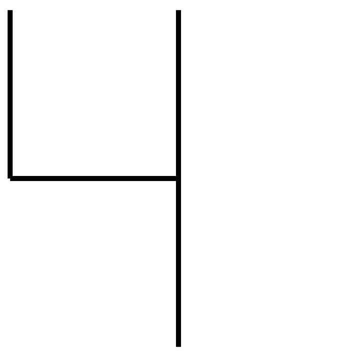
Figure 1: Y-Sign Graph

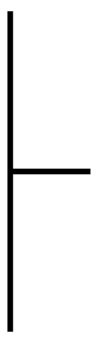
Figure 2: Graph [2,90,1,90,2]

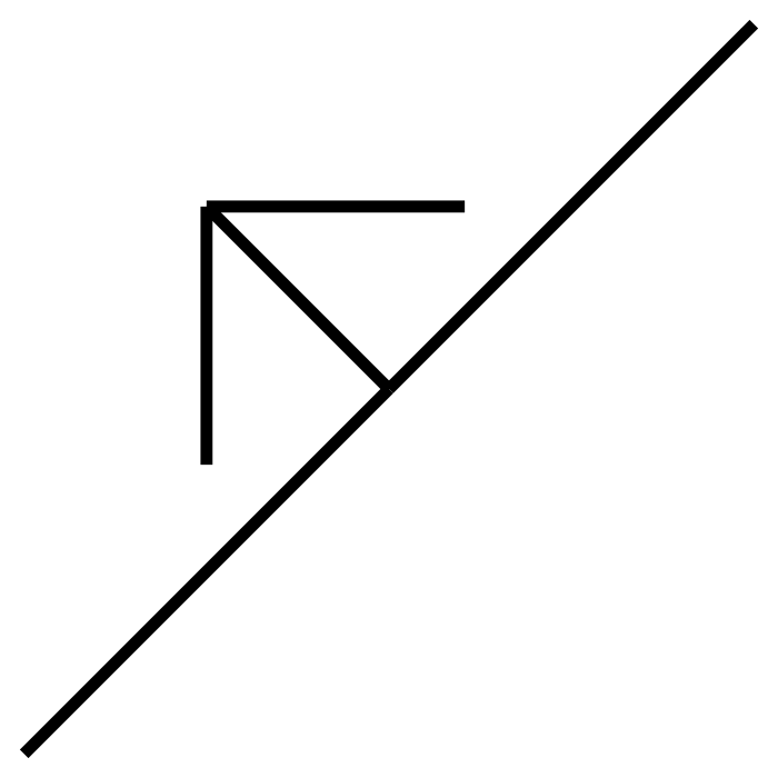
Figure 3: Graph [2,90,1-I,90,2], [3,45,3-I,45,3]

Figure 4: Graph [2-I,90,1,90,2], [3,45,3-I,45,3]

2.4 Node-Centric Representation of Graphs Using Half-Lines

Through exhaustive initial experiments we found that for the encoding and generation of mason’s marks a node-centric (vertex-centric) representation of their underlying connected straight-line graph is helpful. The constraint for a node is defined as follows:

 node(NodePoint, NodeList)
 NodePoint ::= Number-Number
 NodeList  ::= [LineLength] ; [LineLength,Angle|NodeList]

Each node is at the center of several lines leaving it. We record the length of these lines and the angle between neighboring lines. NodeList is a list with elements that are alternating between line lengths and angles, starting and ending in a line length. We may omit the NodePoint and just use node(NodeList). For example node([2,90,1,90,2]) depicts the graph given in Figure 4. Note that each such node forms a small subgraph by itself.

In order to describe larger connected graphs, the node data structure representation is extended to allow identifiers for lines. These identifiers are optionally attached to the line-lengths. If such an identifier is shared between two lines in different nodes it means that these lines are the same, with the two nodes as endpoints. Such annotated lines we call half-lines, because one needs a matching pair of them to form a valid line.

When the nodes are translated into line constraints, the subgraphs of the two nodes connected by this common line are scaled and rotated such that the half-lines become identical. For example node([2,90,1-I,90,2]), node([3,45,3-I, 45,3]) depicts the graph given in Fig. 4. In effect, the subgraph node([3,45,3-I, 45,3]) is rotated and scaled to meet the half-line in node([1,45,1-I,45,1]). Contrast this with the situation in Figure 4, where the half line of the first node has changed.

2.5 Exhaustive Generation of Arbitrary Graphs

We can exhaustively generate graphs from a given node-centric representation containing half-lines with free unbound logical variables as identifiers. Different resulting graphs are possible, depending on which half-lines are identified by binding (aliasing) their variables. Not all such matchings lead to a valid graph, because the resulting graph may not be geometrically possible.

In our implementation, the given graph in node-centric representation is translated into a conjunction of lines (some of them are half-lines). First, all identifiers of half-lines are collected into a list. The identifiers can be unbound variables, in that case identifiers can be bound to each other, making them equivalent. Then a recursion on this list using Prolog predicate pairlines equates the next identifier in the list with one of the remaining identifiers using the Prolog built-in select(Element,List,RestList) that non-deterministically removes an element from a list. Recursion continues with the remaining list L1.

pairlines([I|L]) :- select(I,L,L1), pairlines(L1).
pairlines([]).

Two half-lines with identical identifiers react with each other by following rule. The purpose of the rule is to connect the two subgraphs in which the two half-lines occur by merging the two lines into one. Essentially the same non-deterministic paring rules were used in different application domain in [FB98]. Scaling and rotation is applied to the complete subgraph in which the second half-line occurs using the constraint update(Node,Scaling,Rotation). Finally, the nodes of the two half lines are identified and a new proper full line without identifier replaces the two merged half-lines. (At this point, the node points are still unbound variables, their coordinates have no values yet.)

 % find two half-lines whose half-line identifier is the same
 % to connect their subgraphs
l(N1,N2,M1-I,A1), l(N3,N4,M2-I,A2) <=>
    alldiff([N1,N2,N3,N4]),     % all nodes must be different
    M is M1/M2, A is A1+180-A2, % compute scaling and rotation
    update(N3,M,A), % scale and rotate N3 graph to fit N1 graph
    N1=N4, N2=N3,   % equate nodes of now identical half-lines
    l(N1,N2,M1,A1). % merged line replaces the two half-lines

The rule for updating a line by constraint update(Node,Scaling,Rotation) using scaling and rotation and for updating all lines connected to that line is shown below. It has to avoid repeated updates of the same line. Therefore the update removes the line and produces an intermediate representation of the line using constraint lu.

 % update line with node N1 by scaling and rotation
update(N1,M,A) \ l(N1,N2,M1,A1) <=>  numbers(M1,A1) |
     M2 is M1*M, A2 is A+A1,
     lu(N1,N2,M2,A2),  % intermediate updated line
     update(N2,M,A).   % propagate update to node N2
 % same for line with node N2 to update

This simpagation rule keeps the update constraint but removes the line constraint l. It is replaced by the updated line constraint lu and the update is also applied to node N1. Only when all updates are done, all these intermediate lu lines are replaced by original l lines with the help of some additional rules.

2.6 Random Generation of Graphs for Mason Marks

We have encoded a number of mason’s marks from [Rži81] in our node-centric representation, in particular for the Ulm Minster (see Figure 5). The minster has thousands of marks of about 120 different designs. Most of these marks can be described using just 4 to 5 node constraints in our node-centric representation. In each mason’s mark there is typically a node that is connected to most nodes and that is located near the geometric center of the mason’s mark. Such a node is heuristically chosen as the primary node of the mason’s mark graph. We collected all node constraints for primary nodes and for all other nodes from our encoding of existing mason’s marks.

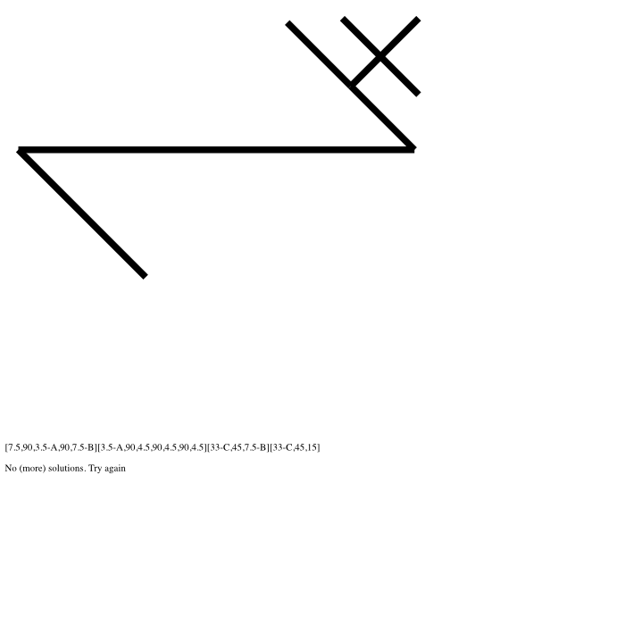
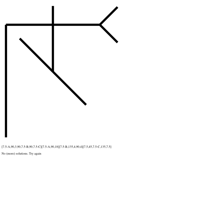
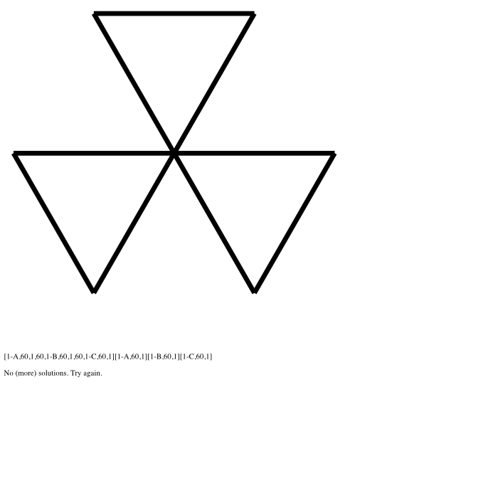
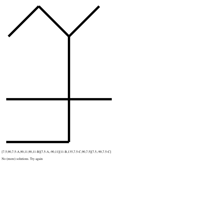
Figure 5: Mason’s Marks of Ulm Minster

For random generation of similarly shaped mason’s mark graphs, first we choose one primary node and two other nodes randomly, and then check if their angles are either multiples of 30 or 45 degrees. If so, we choose a fourth node from the remaining other nodes (ignoring duplicates). The resulting graph may not be valid due to unmatched half-lines. We then use Prolog’s backtracking to try all possible fourth nodes. In this way, zero, one or more valid mason’s marks are randomly produced from the given sub-graph nodes. Figure 6 shows some examples of mason’s marks generated in this way.

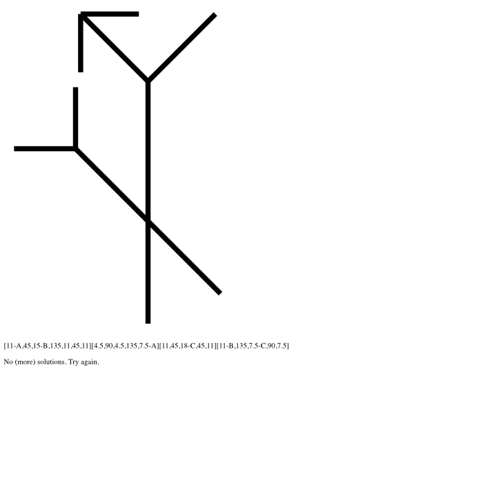
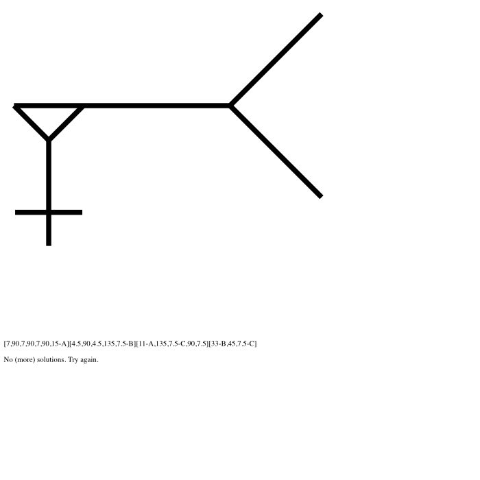
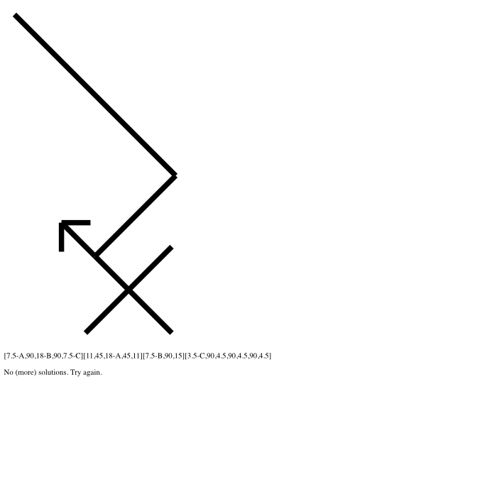
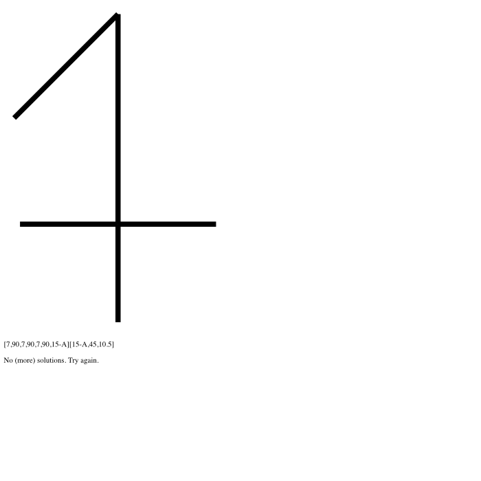
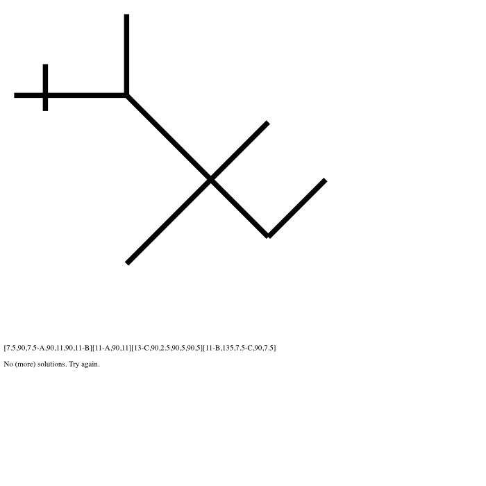
Figure 6: Randomly Generated Mason’s Marks Derived from Ulm Minster Marks

3 Related Work

To the best of our knowledge our work is the first that not only represents, but also analyses and generates mason’s marks. The only related work we could find is [KMMS02]. Given a prototype graph of a mason’s mark and the skeleton graph of an input image, the recognition of this image is considered as search of matchings paths in the skeleton graph with a minimal number of mismatchings. It is not clear from the description of the algorithm how it accounts for scaling and rotation. In contrast, our recognition rules match line edges directly, independent of scale and rotation. Efficiency of matching relies on optimizations of the CHR compiler such as indexing. Imprecision could be taken into account and controlled by rounding the numerical values of coordinates, lengths and angles or by using interval arithmetics.

In the work [Dür96] structural character descriptions for East Asian ideograms (Kanji font characters) are analyzed and generated. Sketches of characters are produced from a symbolic coordinate free description, which is a system of constraints. The authors developed a special finite domain constraint solving algorithm tailored to the problem in CHR. This approach proved to be more efficient and versatile than using existing built-in solvers. Kanji characters are decomposed into subfigures and those are described by strokes (lines) called bars. The representation of bars is similar to our node-centric representation. However, their work employs only the four main directions and lengths are always implicit, while we allow for arbitrary angles and arbitrary explicit lengths.

4 Conclusions and Future Work

We have shortly presented our prototype tool to analyse, generate and draw straight-line graphs based on a novel node-centric representation of graphs using constraints. We have applied the tool to the domain of stonemason’s marks. For a more complete coverage of mason’s marks, we need to add the representation of arcs and other curves. We currently work on representing the mason’s marks found on buildings in the Alicante province in Spain, because these have not been encoded so far.

There is a similarity between our node-centric approach for mason’s marks and the representation of chemical structures using molecules with their bindings. We therefore think that our approach can readily be applied to model and analyse chemical compounds as straight-line graphs. Another application area might be the visualization of temporal constraint networks [Frü94].

References

- [Dav54] Ralph Henry Carless Davis. A catalogue of masons’ marks as an aid to architectural history. Journal of the British Archaeological Association, 17(1):43–76, 1954.
- [Dür96] Martin J. Dürst. Prolog for structured character description and font design. The Journal of Logic Programming, 26(2):133–146, Feb 1996.
- [FB98] Thom Frühwirth and Pascal Brisset. Optimal placement of base stations in wireless indoor telecommunication. In International Conference on Principles and Practice of Constraint Programming, pages 476–480. Springer, 1998.
- [Fol10] Ken Follett. The Pillars of the Earth. Penguin, 2010.
- [Fri32] Karl Friedrich. Die Steinbearbeitung in ihrer Entwicklung vom 11. bis zum 18. Jahrhundert. Filser, 1932. Reprint Aegis Ulm 1988.
- [Frü94] Thom Frühwirth. Temporal reasoning with Constraint Handling Rules. Technical Report ECRC-94-5, European Computer-Industry Research Centre, Munchen, Germany, 1994.
- [Frü09] Thom Frühwirth. Constraint Handling Rules. Cambridge University Press, 2009.
- [Frü15] Thom Frühwirth. Constraint Handling Rules – What Else? In Rule Technologies: Foundations, Tools, and Applications, pages 13–34. Springer International Publishing, 2015.
- [KMMS02] V. Kiiko, V. Matsello, H. Masuch, and G. Stanke. Recognition of mason marks images, found on Citeseer, 2002.
- [Rži81] Franz von Ržiha. Studien über Steinmetz-Zeichen. Kaiserlich-Königliche Hof-und Staatsdruckerei, 1881. Reprint Bau-Verlag 1989.
- [Tam13] Roberto Tamassia. Handbook of graph drawing and visualization. CRC press, 2013.
- [WDKTF14] Jan Wielemaker, Leslie De Koninck, Markus Triska, and Thom Frühwirth. SWI Prolog Reference Manual 7.1. BOD, 2014.