Probing higher-order transitions through scattering of microwave photons in the ultrastrong-coupling regime of circuit QED

Abstract

Higher-order transitions can occur in the ultrastrong-coupling regime of circuit QED through virtual processes governed by the counter-rotating interactions. We propose a feasible way to probe higher-order transitions through the scattering of propagating microwave photons incident on the hybrid qubit-cavity system. The lineshapes in the scattering spectra can indicate the coherent interaction between the qubits and the cavity, and the higher-order transitions can be identified in the population spectra. We further find that if the coupling strengths between the two qubits and the cavity are tuned to be asymmetric, the dark antisymmetric state with the Fano-lineshape can also be detected from the variations in the scattering spectra.

I INTRODUCTION

With the recently advanced development in superconducting quantum circuits (SQCs), investigations of microwave photonics have been extended to circuit quantum electrodynamics (QED) systems You and Nori (2011); Gu et al. (2017); Girvin (2014), in which superconducting artificial atoms and resonators substitute for the essential building blocks (natural atoms and optical cavities) in cavity QED. Superconducting circuit has already been proven as a useful vehicle for the realizations of quantum coherence Chiorescu et al. (2003), quantum information processing, and atomic physics You and Nori (2011), particularly in the regimes not easily accessible with natural atoms and molecules Irish (2007); Ashhab and Nori (2010). In contrast to conventional cavity QED, circuit QED can be artificially designed and fabricated for different research purposes Wallraff et al. (2004); Hime et al. (2006); Niskanen et al. (2007); Buluta1 et al. (2011); Xiang et al. (2013); Gu et al. (2017). The energy levels of superconducting artificial atoms and the oscillator frequency of resonator can be adjusted in a wide range of possible values. The coupling strengths between superconducting artificial atoms and their electromagnetic environments can also be tuned. These flexible circuit designs make circuit QED a promising candidate for exploring microwave quantum optics on a superconducting chip.

The interaction between an atomic system and electromagnetic fields in cavity QED has been widely studied over the past few decades Scully and Zubairy (1999); Hood et al. (1998); Kimble (1998); Mabuchi and Doherty (2002); Hennessy et al. (2007). Analogously, the superconducting artificial atoms in circuit QED can be strongly coupled to quantized microwave fields in the transmission line or 3D resonators You and Nori (2003); Paik et al. (2011); Xiang et al. (2013); Stern et al. (2014); Gu et al. (2017). Just like natural atoms, superconducting artificial atoms are multi-level systems You and Nori (2011). If we limit our study to the two lowest-energy levels, this can be defined as a superconducting qubit. It is known that the coupling strength ($\lambda$) between the superconducting qubit and the resonator field can be experimentally engineered to become comparable to the transition frequencies of the qubit and the resonator ($\omega_{q}$ and $\omega_{c}$, respectively) Niemczyk et al. (2010); Forn-Díaz et al. (2010); Yoshihara et al. (2017); Braumüller et al. (2017); Forn-Díaz et al. (2017). With this extremely strong coupling strength ($\lambda\gtrsim 0.1\omega_{q/c}$) Gu et al. (2017), one can reach the ultrastrong-coupling (USC) regime in circuit QED Gu et al. (2017); Xiang et al. (2013); Nataf and Ciuti (2010); Peropadre et al. (2010); Ridolfo et al. (2012, 2013); Stassi et al. (2013); Garziano et al. (2014, 2015); Ma and Law (2015); Garziano et al. (2016); Kockum et al. (2017); Forn-Díaz et al. (2017); Niemczyk et al. (2010); Forn-Díaz et al. (2010); Yoshihara et al. (2017); Braumüller et al. (2017). In the USC regime, higher-order atom-field resonant transitions can occur via virtual processes, which do not conserve the number of excitationsXiang et al. (2013); Gu et al. (2017); Stassi et al. (2013); Garziano et al. (2014, 2015); Ma and Law (2015); Garziano et al. (2016); Kockum et al. (2017). These processes governed by the counter-rotating terms in the interaction Hamiltonian can no longer be neglected, and therefore the rotating wave approximation (RWA) breaks down .

Circuit QED is a promising tool to generate single microwave photons Houck et al. (2007) and also paves the way to study the scattering properties of single microwave photons propagating in the circuit Romero et al. (2009); Peropadre et al. (2011). Based on this feature, several theoretical works Shen and Fan (2005); Zhou et al. (2008); Shen and Fan (2009); Witthaut and Sorensen (2010); Chen et al. (2014); Roy et al. (2017) have been proposed to study the response of injected microwave photons travelling in the transmission line. When a propagating microwave photon is coupled to an emitter, the interaction gives rise to the scattering of the field or the excitation of the emitter. The phenomenon leads to the variations of the profile in the scattering spectra Shen and Fan (2005); Zhou et al. (2008); Shen and Fan (2009); Witthaut and Sorensen (2010); Chen et al. (2014); Roy et al. (2017); Chang et al. (2007); Chen et al. (2011a, b); Chen and Chen (2012); Chen (2016); Kuo et al. (2016). Therefore, one can use this advantage to measure the qubit states through the detection of the transmitted/reflected photons. While most of the previous studies are focused in the weak- or strong-coupling regimes, in this work, however, we aim to study the scattering spectra of a superconducting circuit system comprising the transmission line resonator coupled to two superconducting charge qubits in the USC regime. The main purpose of this work is to observe the higher-order resonant transitions in populations through the scattering of microwave photons incident on the qubit-cavity system. Moreover, we also find that the dark antisymmetric state in the higher-order transitions can be probed if the coupling strengths between the qubits and the cavity are tuned to be asymmetric. Our consideration provides an experimentally feasible way to detect the higher-order resonant transitions in the USC regime.

II THE MODEL

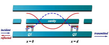
Figure 1: (Color online) Schematic diagram of two charge qubits coupled to a resonator in a transmission-line waveguide. A microwave photon incident from the left is coherently scattered by the qubit-cavity system.

We investigate a general one-dimensional model with two identical superconducting qubits, separated by a distance $d$ and embedded in a transmission-line waveguide, coupled to a cavity as depicted in Fig. 1. We first consider a simple two-level configuration for the two qubits consisting of the ground and the excited states ($|g\rangle,|e\rangle$) with the transition frequency $\omega_{q}$. The cavity with the resonance frequency $\omega_{c}$ is formed by two capacitive gaps in the middle conductor. We assume that an incident microwave photon with energy $E_{k}=\hbar v_{g}k$ propagating in the transmission line from the left would be either scattered or absorbed by the qubits. Here, $v_{g}$ and $k$ are the group velocity and wave vector, respectively. The Hamiltonian describing the system can be transformed into real space as $H=H_{wg}+H_{I}+H_{\textrm{cav}}$, where $H_{\textrm{wg}}$ is the Hamiltonian of the waveguide in which photons propagate, $H_{I}$ describes the interaction between the propagating photons and the two separated identical qubits, and $H_{\textrm{cav}}$ represents the Hamiltonian of a singl-mode microwave cavity field interacting with the two qubits as shown in the following equations Garziano et al. (2016); Chen et al. (2011a).

$$H_{\textrm{wg}}/\hbar =\int dx(-iv_{g})C_{R}^{{\dagger}}(x)\frac{\partial}{\partial x}C_{R}(x)$$ (1a)

$$+\int dx(iv_{g})C_{L}^{{\dagger}}(x)\frac{\partial}{\partial x}C_{L}(x),$$

$$H_{I}/\hbar =g\int dx\sum_{j=1,2}\delta\Big{[}x-(j-1)d\Big{]}\times$$ (1b)

$$\Big{[}C_{R}^{{\dagger}}(x)\sigma_{-}^{(j)}+C_{R}(x)\sigma_{+}^{(j)}+C_{L}^{{\dagger}}(x)\sigma_{-}^{(j)}+C_{L}(x)\sigma_{+}^{(j)}\Big{]},$$

$$H_{\textrm{cav}}/\hbar =\omega_{q}\sum_{j=1,2}\sigma_{e_{j},e_{j}}+\omega_{c}a^{{\dagger}}a$$ (1c)

$$+\sum_{j=1,2}\lambda_{j}(a+a^{\dagger})(\cos\theta\sigma_{x}^{(j)}+\sin\theta\sigma_{z}^{(j)}).$$

In Eq. (1a), $C_{R}^{{\dagger}}(x)\ [C_{L}^{{\dagger}}(x)]$ denotes a bosonic operator creating a right-going (left-going) photon at x. In Eq. (1b), $\sigma_{+}^{(j)}=|e_{j}\rangle\langle g_{j}|\ (\sigma_{-}^{(j)}=|g_{j}\rangle\langle e_{j}|)$ represents the raising (lowering) operator of the $jth$ qubit, while $g$ is the coupling strength between the two qubits and the waveguide photon. The first two terms in Eq. (1c) denote the free Hamiltonians of the qubits and the cavity field with the frequency $\omega_{q}$ and $\omega_{c}$. The last term describes the interaction between the $jth$ qubit and the cavity field with the coupling strength $\lambda_{j}$. The diagonal element of the $jth$ qubit can be represented as the form of $\sigma_{e_{j},e_{j}}=|e_{j}\rangle\langle e_{j}|$, and $a^{{\dagger}}$ ($a$) is the creation (annihilation) operator for the cavity photon, while $\sigma_{x}^{(j)}$ and $\sigma_{z}^{(j)}$ are Pauli matrices for the $jth$ qubit. One notes that, in this work, we consider the superconducting circuit operating in the USC regime with the qubit-cavity coupling strength $\lambda\geq 0.1\omega_{q}$. The RWA is therefore not valid in the USC regime. Analyzing the properties of the qubits and the cavity in this regime requires the full quantum Rabi Hamiltonian. The Hamiltonian in Eq. (1c) contains the counter-rotating terms, which do not conserve the number of excitations with the form $\sigma_{+}^{(j)}a^{{\dagger}}$, $\sigma_{-}^{(j)}a$, $\sigma_{z}^{(j)}a^{{\dagger}}$, and $\sigma_{z}^{(j)}a$.

The stationary state of the system can be written as

$$|E_{k}\rangle =\sum_{m=R,L}\sum_{i=1,2}\int dx\phi_{k,m}^{\dagger}(x)C_{m}^{\dagger}$$ (2)

$$\times\Big{[}(1+a^{{\dagger}}+a^{{\dagger}}a^{{\dagger}})(1+\sigma_{+}^{(i)}+\sigma_{+}^{(1)}\sigma_{+}^{(2)})\Big{]}|\textrm{vac}\rangle$$

$$+(1+a^{{\dagger}}+a^{{\dagger}}a^{{\dagger}})$$

$$\times\sum_{i=1,2}\sum_{j=0,1,2}\Big{[}\alpha_{i,j}\sigma_{+}^{(i)}+\beta_{j}\sigma_{+}^{(1)}\sigma_{+}^{(2)}\gamma_{j}\Big{]}|\textrm{vac}\rangle,$$

where $|\textrm{vac}\rangle=|g_{1},g_{2}\rangle|0\rangle_{\textrm{cav}}|0\rangle_{\textrm{wg}}$ is the vacuum state with both the superconducting qubits in their ground states and zero photon in both the cavity and the waveguide. Hereafter, we use a simplified notation for the quantum states in this system, for example, $|\textrm{vac}\rangle=|gg00\rangle$. In Eq. (2), $\alpha_{i,j},\beta_{j},and\gamma_{j}$ are the probability amplitudes of each state: $\alpha_{i,j}$ represents the probability amplitude that the $ith$ qubit absorbs photon energy and jumps to its excited state with $j$ photons existing in the cavity, $\beta_{j}$ indicates the probability amplitude that both the qubits absorb photon energy and jump to their excited states with $j$ photons existing in the cavity, and $\gamma_{j}$ denotes the probability amplitude that no qubits absorb photon energy and remain in their ground states with $j$ photons in the cavity. We assume that one photon is incident from the left of the waveguide, the scattering occurs at the position of the two qubits due to their interactions with the incident photon. The scattering amplitude wave function $\phi_{k,R}^{\dagger}(x)$ and $\phi_{k,L}^{\dagger}(x)$ take the form

$$\left\{\begin{aligned} \phi_{k,R}^{{\dagger}}(x)&\equiv exp(ikx)[\theta(-x)+a\theta(x)\theta(d-x)+t\theta(x-d)],\\ \phi_{k,L}^{{\dagger}}(x)&\equiv exp(-ikx)[r\theta(-x)+b\theta(x)\theta(d-x)],\end{aligned}\right.$$ (3)

where $t$ and $r$ are the transmission and reflection amplitudes, respectively. Here, $a$ and $b$ represent the probability amplitudes of the photon between $x=0$ and $x=d$, while $\theta(x)$ is the unit step function.

In the USC regime, the presence of the counter-rotating terms in the $H_{\textrm{cav}}$ enables four different paths which envolve from the initial state $|gg10\rangle$ to the final state $|ee00\rangle$ via several intermediate virtual states Garziano et al. (2016), such as $|ee10\rangle,\ |eg20\rangle,\ |eg10\rangle,\ |eg00\rangle,\ |ge20\rangle,|ge10\rangle,\ |ge00\rangle,\\ \ |gg20\rangle,$ and$\ |gg00\rangle$. Without loss of generality, we limit the total Hamiltonian $H$ and the eigenstate $|E_{k}\rangle$ to the 3-excitation manifold. The Hamiltonian can then be spanned (as shown in Appendix A) by the bases: $\{|ee10\rangle,\ |ee00\rangle,\ |eg20\rangle,\ |eg10\rangle,\ |eg00\rangle,\ |ge20\rangle,\ |ge10\rangle,\\ |ge00\rangle,\ |gg20\rangle,\ |gg10\rangle,\ |gg01\rangle_{R}\ (|gg01\rangle_{L}),$ and$\ |gg00\rangle\}$. By solving the time-independent eigenvalue equation $H|E_{k}\rangle=E_{k}|E_{k}\rangle$, one can obtain the following relations for the coefficients:

$$\left\{\begin{aligned} t&=1+\frac{g}{iv_{g}}\Big{[}\alpha_{10}+\alpha_{20}~{}exp(-ikd)\Big{]},\\ r&=\frac{g}{iv_{g}}\Big{[}\alpha_{10}+\alpha_{20}~{}exp(ikd)\Big{]},\\ a&=\frac{g}{iv_{g}}\alpha_{10}+1,\\ b&=\frac{g}{iv_{g}}\alpha_{20}~{}exp(ikd).\end{aligned}\right.$$ (4)

The transmission and reflection amplitudes of the incident microwave photon can then be determined algebraically.

III RESULTS AND DISCUSSIONS

III.1 Higher-order transitions

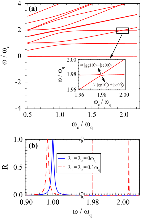
Figure 2: (Color online) (a) The figure shows the energy levels for the lowest energy eigenstates of the qubit-cavity system as a function of the normalized cavity frequency $\omega_{c}/\omega_{q}$, using the parameters $\lambda_{1}=\lambda_{2}=0.1\omega_{q}$ and $\theta=\pi/6$, where $\omega_{q}$ is the qubit frequency as a reference point. In the inset, we can observe the anticrossing between $|gg10\rangle$ and $|ee00\rangle$, adopted from Garziano et al. (2016). (b) The reflection spectra R of the incident microwave photons in a one-dimensional waveguide for the coupling strengths: $\lambda_{1}=\lambda_{2}=0\omega_{q}$ (blue-solid curve) and $\lambda_{1}=\lambda_{2}=0.1\omega_{q}$ (red-dashed curve).

After numerically diagonalizing the Hamiltonian in Eq. (1c), the energy levels as a function of the normalized cavity frequency ($\omega_{c}/\omega_{q}$) can be plotted as shown in Fig. 2(a). In the region around $\omega_{c}/\omega_{q}=2$, a splitting anti-crossing can be observed at energy level $\omega/\omega_{q}\approx 2$ (marked by the black square). It has been reported Garziano et al. (2016) that the avoided-crossing level [see the inset in Fig. 2(a)] demonstrateing the coupling between the states $|gg10\rangle$ and $|ee00\rangle$ in the USC regime. The interaction does not conserve the number of excitations due to the presence of the counter-rotating terms in the system Hamiltonian. This indicates that if the coupling strength between the qubits and the cavity is sufficiently strong with the frequency of the cavity being double the qubit transition frequency, single photon is able to excite two qubits simultaneously to their excited states even though the cavity is initially in one-photon state Garziano et al. (2016).

We now propose a way to feasibly probe the higher-order transitions through the scattering of the microwave photons incident on the hybrid qubit-cavity system. Figure. 2(b) shows the reflection spectra $R=|r|^{2}$ for different coupling strengths $\lambda$ as a function of the normalized microwave photon frequency. We consider the coupling strengths between each qubit and the cavity field, $\lambda_{1}$ and $\lambda_{2}$, are the same under the condition of $\omega_{c}/\omega_{q}=2$. As can be seen, when the interaction between the qubits and the cavity vanishes, i.e. $\lambda_{1}=\lambda_{2}=0$, the peak of the blue-solid curve is on resonance with the qubits. The qubits act like a perfect mirror with total reflection of the incident microwave photons. However, when the couplings are present with $\lambda_{1}=\lambda_{2}$, the profile of $R$ (red-dashed curve, with $\lambda_{1}=\lambda_{2}=0.1\omega_{q}$) shows three peaks at the normalized microwave photon frequency ($\omega/\omega_{q}$) around 0.98, 1.98, and 2.004.

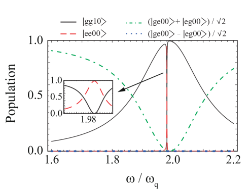
Figure 3: (Color online) The populations of the energy eigenstates. The parameters $\lambda_{1}$, $\lambda_{2}$, $g$, $\Gamma=\dfrac{4g^{2}}{v^{2}}$ (the decay rate into the microwave photon modes), and $\omega_{c}$ are normalized to the qubit frequency $\omega_{q}$. We set $\lambda_{1}=\lambda_{2}=0.1\omega_{q}$, $g=0.05\omega_{q}$, $\Gamma=0.005\omega_{q}$, and $\omega_{c}=2\omega_{q}$. The black-solid, red-dashed, green-dot-dashed ,and blue-dotted curves represent the states $|gg10\rangle$, $|ee00\rangle$, $(|ge00\rangle+|eg00\rangle)/\sqrt{2}$, and $(|ge00\rangle-|eg00\rangle)/\sqrt{2}$, respectively. In the inset, we can observe the populations of $|ee00\rangle$ and $|gg10\rangle$ exchange at the normalized frequency near 1.98.

Figure. 3 shows the populations of the energy eigenstates as a function of the normalized microwave photon frequency. By comparing Fig. 2(b) with Fig. 3, one can find that the first peak at the normalized frequency around 0.98 corresponds to the symmetric state Garziano et al. (2016) $(|ge00\rangle+|eg00\rangle)/\sqrt{2}$. When the interaction between the qubits and the cavity exists, the microwave photon can be absorbed by the qubit-cavity system and create one photon in the cavity to form one bare state $|gg10\rangle$. For the frequency of the cavity being double the qubit transition frequency, the bare state $|gg10\rangle$ (black-solid curve) takes all the excitation at the normalized frequency 2.004. Since the initial state $|gg10\rangle$ evolves to the final state $|ee00\rangle$ with the virtual processes Garziano et al. (2016), we can see that the populations of $|ee00\rangle$ (red-dashed curve) and $|gg10\rangle$ exchange at the normalized frequency near 1.98 in Fig. 3. Therefore, the second and the third red peaks in Fig. 2(b) can be identified as the states $|ee00\rangle$ and $|gg10\rangle$, respectively. The relation reveals that through the scattering of the microwave photons, one can detect not only the existence of the qubit-cavity interaction, but also the variations of the energy eigenstates by tuning the frequencies of the microwave photons.

III.2 Dark antisymmetric state

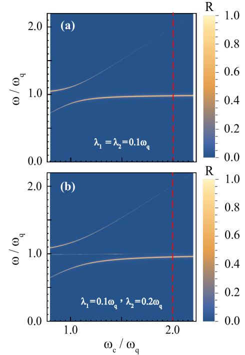
Figure 4: (Color online) Figure (a) and (b) are the density plots of the reflection spectra R of the incident microwave photons as functions of $\omega_{/}\omega_{q}$ and $\omega_{c}/\omega_{q}$. The bright regions indicate the high reflection probability around 1. The coupling strengths between the qubits and the cavity are choosen as $\lambda_{1}=\lambda_{2}=0.1\omega_{q}$ in (a) and $\lambda_{1}=0.1\omega_{q},\lambda_{2}=0.2\omega_{q}$ in (b).

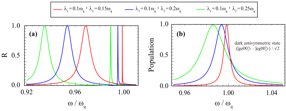
Figure 5: (Color online) (a) The reflection spectra R for the asymmetric coupling strengths between the two qubits and the cavity as a function of the normalized microwave photon frequency. (b) The populations of the dark antisymmetric state $(|ge00\rangle-|eg00\rangle)/\sqrt{2}$ as a function of the normalized microwave photon frequency. The red, blue, and green curves denote $(\lambda_{1}=0.1\omega_{q},~{}\lambda_{2}=0.15\omega_{q})$, $(\lambda_{1}=0.1\omega_{q},~{}\lambda_{2}=0.2\omega_{q})$, and $(\lambda_{1}=0.1\omega_{q},~{}\lambda_{2}=0.25\omega_{q})$, respectively.

In Fig. 2(a), the straight line at $\omega/\omega_{q}\approx 1$ corresponds to the dark antisymmetric state Garziano et al. (2016) $(|ge00\rangle-|eg00\rangle)/\sqrt{2}$. However, the reflection spectra in the density plot shown in Fig. 4(a) does not exhibit this line for the dark state when $\lambda_{1}=\lambda_{2}$. The reason is that the dark state can not absorb/emit photons when $\lambda_{1}=\lambda_{2}$. Nevertheless, if the values of $\lambda_{1}$ and $\lambda_{2}$ are tuned to be asymmetric, for example, $\lambda_{1}=0.1\omega_{q}$ and $\lambda_{2}=0.2\omega_{q}$, the line representing the dark state appears at $\omega/\omega_{q}\approx 1$ as shown in Fig. 4(b). This is because the difference between the coupling strengths $\lambda_{1}$ and $\lambda_{2}$ changes the eigenvalues, such that the dark state is no longer ”dark” and can absorb/emit photons. Along the red-dashed lines placed at $\omega_{c}/\omega_{q}=2$ in Figs. 4(a) and 4(b), we can plot the corresponding reflection spectra as a function of the normalized microwave photon frequency as shown in Fig. 2(b) [red-dashed curve] and Fig. 5(a) [blue-solid curve], respectively. In contrast to the red-dashed curve ($\lambda_{1}=\lambda_{2}=0.1\omega_{q}$) in Fig. 2(b), each curve in Fig. 5(a) shows an extra Fano-like lineshape located at $\omega/\omega_{q}\approx 1$ due to the difference between $\lambda_{1}$ and $\lambda_{2}$. The Fano lineshapes are more distinct when $\lambda_{2}$ is close to $\lambda_{1}$, and the peaks of the Fano lineshapes shift to left as the values of $\lambda_{2}$ increase. Figure 5(b) displays the populations of the dark antisymmetric states [$(|ge00\rangle-|eg00\rangle)/\sqrt{2}$] for different asymmetric coupling strengths between the two qubits and the cavity. Here, the value of $\lambda_{1}$ is fixed at $0.1\omega_{q}$, and the values of $\lambda_{2}$ are chosen as $1.5\omega_{q}$, $2.0\omega_{q}$, and $2.5\omega_{q}$ (red, blue, and green curves, respectively). When the values of $\lambda_{2}$ are not equal to $\lambda_{1}$, one can find that the dark antisymmetric states show the Lorentzian lineshapes and the populations can reach unity. This is totally different from the zero popultion of the truely dark antisymmetric state (blue-dotted curve) in Fig. 3. The peaks of the Lorentzian lineshapes also shift to left as the values of $\lambda_{2}$ increase. The trend coincides with the Fano lineshapes in Fig. 5(a). The Fano resonance can occur when the localized channel (discrete state) interfere with the the delocalized channel (continuum) Miroshnichenko et al. (2010); Chen et al. (2017); Kuo et al. (2016). Here, the Lorentzian lineshapes of the dark antisymmetric states in Fig. 5(b) represent the localized channel, and the microwave photons stand for the delocalized channel. The curves in Fig. 5(a) therefore exhibit asymmetric lineshapes of the Fano resonance at $\omega/\omega_{q}\approx 1$.

The above results show that, by analyzing the scattering spectra, one can probe the higher-order resonant transitions stemming from the interplay of the energy levels in the USC regime. Experimentally, the coupling strengths between the qubits and the microwave photons can be tuned by changing the magnetic flux and the gate voltage, and the detuning between the transition frequency of the qubit and the microwave photons can be also changed in a similar way.

IV CONCLUSION

In conclusion, we investigate the superconducting circuit system consisting of two charged qubits coupled to the cavity in a transmission-line waveguide in the USC regime. We propose that through the scattering of the microwave photons incident on the qubit-cavity system, one can probe higher-order qubit-cavity resonant transitions which do not conserve the number of excitations and cannot be observed in the weak- and strong-coupling regimes. We further show that by tuning the two coupling strengths $\lambda_{1}$ and $\lambda_{2}$ properly, the dark antisymmetric state with the Fano lineshape can be also detected in the scattering spectra. Our proposal provides an experimentally feasible way to observe the interesting phenomena in the USC regime.

Appendix A Analytical calculations of the transmission and reflection amplitudes

In this appendix, we present the full calculations for solving the time-independent eigenvalue equation $H|E_{k}\rangle=E_{k}|E_{k}\rangle$. First, we represent the Hamiltonian in Eq. (1) with the matrix form as shown below. In Eq. (5), $H_{R}$ describes the total Hamiltonian with an incident microwave photon propagating in right direction, while $H_{L}$ describes the Hamiltonian that a microwave photon propagates to left direction. The bases from left to right in both $H_{R}$ and $H_{L}$ are $|ee10\rangle,\ |ee00\rangle,\ |eg20\rangle,\ |eg10\rangle,\ |eg00\rangle,\ |ge20\rangle,\ |ge10\rangle,\ |ge00\rangle,\ |gg20\rangle,\ |gg10\rangle,\ |gg01\rangle_{R/L},$ and$\ |gg00\rangle$.

$$H_{R}/\hbar=\left(\begin{array}[]{cccccccccccc}C_{4}&C_{9}&\sqrt{2}C_{8}&0&C_{8}&\sqrt{2}C_{7}&0&C_{7}&0&0&0&0\\ C_{9}&2C_{2}&0&C_{8}&0&0&C_{7}&0&0&0&0&0\\ \sqrt{2}C_{8}&0&C_{5}&\sqrt{2}C_{10}&0&0&0&0&0&\sqrt{2}C_{7}&0&0\\ 0&C_{8}&\sqrt{2}C_{10}&C_{6}&C_{10}&0&0&0&\sqrt{2}C_{7}&0&0&C_{7}\\ C_{8}&0&0&C_{10}&C_{2}&0&0&0&0&C_{7}&k_{2}&0\\ \sqrt{2}C_{7}&0&0&0&0&C_{5}&-\sqrt{2}C_{10}&0&0&\sqrt{2}C_{8}&0&0\\ 0&C_{7}&0&0&0&-\sqrt{2}C_{10}&C_{6}&-C_{10}&\sqrt{2}C_{8}&0&0&C_{8}\\ C_{7}&0&0&0&0&0&-C_{10}&C_{2}&0&C_{8}&k_{2}&0\\ 0&0&0&\sqrt{2}C_{7}&0&0&\sqrt{2}C_{8}&0&2C_{3}&-\sqrt{2}C_{9}&0&0\\ 0&0&\sqrt{2}C_{7}&0&C_{7}&\sqrt{2}C_{8}&0&C_{8}&-\sqrt{2}C_{9}&C_{3}&0&-C_{9}\\ 0&0&0&0&k_{2}&0&0&k_{2}&0&0&C_{1}k_{1}&0\\ 0&0&0&C_{7}&0&0&C_{8}&0&0&-C_{9}&0&0\end{array}\right),$$ (5a)

$$H_{L}/\hbar=\left(\begin{array}[]{cccccccccccc}0&0&0&0&0&0&0&0&0&0&0&0\\ 0&0&0&0&0&0&0&0&0&0&0&0\\ 0&0&0&0&0&0&0&0&0&0&0&0\\ 0&0&0&0&0&0&0&0&0&0&0&0\\ 0&0&0&0&0&0&0&0&0&0&k_{2}&0\\ 0&0&0&0&0&0&0&0&0&0&0&0\\ 0&0&0&0&0&0&0&0&0&0&0&0\\ 0&0&0&0&0&0&0&0&0&0&k_{3}&0\\ 0&0&0&0&0&0&0&0&0&0&0&0\\ 0&0&0&0&0&0&0&0&0&0&0&0\\ 0&0&0&0&k_{2}&0&0&k_{3}&0&0&-C_{1}k_{1}&0\\ 0&0&0&0&0&0&0&0&0&0&0&0\\ \end{array}\right),$$ (5b)

with the values $C_{1}$ to $C_{10}$ and $k_{1}$ to $k_{3}$ defined as

$$\left\{\begin{array}[]{lll}C_{1}=-i\Gamma\dfrac{v^{2}}{4g^{2}}&,C_{2}=1&,C_{3}=\delta,\\ C_{4}=2+\delta&,C_{5}=1+2\delta&,C_{6}=1+\delta,\\ C_{7}=\lambda_{a}\cos\theta&,C_{8}=\lambda_{b}\cos\theta&,C_{9}=(\lambda_{a}+\lambda_{b})\sin\theta,\\ C_{10}=(\lambda_{a}-\lambda_{b})\sin\theta,\\ k_{1}=\int\frac{\partial}{\partial x}dx&,k_{2}=\int g\delta(x)dx&,k_{3}=\int g\delta(x-d)dx.\end{array}\right.$$

Note that $C_{1}$ to $C_{10}$ are all normalized to the qubit frequency $\omega_{q}$, and therefore $\lambda_{a}$, $\lambda_{b}$, and $\delta$ represent $\lambda_{1}/\omega_{q}$, $\lambda_{2}/\omega_{q}$, and $\omega_{c}/\omega_{q}$, respectively.

The stationary eigenstates of the system can be written with the matrix form:

$$|E_{k}\rangle_{R}=\left(\begin{array}[]{cccccccccccc}\beta_{1}\\ \beta_{0}\\ \sqrt{2}\alpha_{12}\\ \alpha_{11}\\ \alpha_{10}\\ \sqrt{2}\alpha_{22}\\ \alpha_{21}\\ \alpha_{20}\\ \sqrt{2}\gamma_{2}\\ \gamma_{1}\\ \phi_{k,R}^{{\dagger}}(x)\\ \gamma_{0}\end{array}\right),|E_{k}\rangle_{L}=\left(\begin{array}[]{cccccccccccc}\beta_{1}\\ \beta_{0}\\ \sqrt{2}\alpha_{12}\\ \alpha_{11}\\ \alpha_{10}\\ \sqrt{2}\alpha_{22}\\ \alpha_{21}\\ \alpha_{20}\\ \sqrt{2}\gamma_{2}\\ \gamma_{1}\\ \phi_{k,L}^{{\dagger}}(x)\\ \gamma_{0}\end{array}\right).$$ (6)

By solving the time-independent Schrödinger equation, $H_{R}|E_{k}\rangle_{R}=E_{k}|E_{k}\rangle_{R}$ and $H_{L}|E_{k}\rangle_{L}=E_{k}|E_{k}\rangle_{L}$, one obtains the following equations:

$$C_{8}\alpha_{10}+2C_{8}\alpha_{12}+C_{7}\alpha_{20}+2C_{7}\alpha_{22}+C_{9}\beta_{0}+(C_{4}-v_{g}k)\beta_{1}=0,$$ (7)

$$C_{8}\alpha_{11}+C_{7}\alpha_{21}+(2C_{2}-v_{g}k)\beta_{0}+C_{9}\beta_{1}=0,$$ (8)

$$\sqrt{2}C_{10}\alpha_{11}+(\sqrt{2}C_{5}-v_{g}k)\alpha_{12}+\sqrt{2}C_{8}\beta_{1}+\sqrt{2}C_{7}\gamma_{1}=0,$$ (9)

$$C_{10}\alpha_{10}+(C_{6}-v_{g}k)\alpha_{11}+2C_{10}\alpha_{12}+C_{8}\beta_{0}+C_{7}\gamma_{0}+2C_{7}\gamma_{2}=0,$$ (10)

$$(C_{2}-v_{g}k)\alpha_{10}+C_{10}\alpha_{11}+C_{8}\beta_{1}+C_{7}\gamma_{1}=-k_{2}\int dx[\phi_{k,R}^{{\dagger}}(x)+\phi_{k,L}^{{\dagger}}(x)],$$ (11)

$$-\sqrt{2}C_{10}\alpha_{21}+(\sqrt{2}C_{5}-v_{g}k)\alpha_{22}+\sqrt{2}C_{7}\beta_{1}+\sqrt{2}C_{8}\gamma_{1}=0,$$ (12)

$$-C_{10}\alpha_{20}+(C_{6}-v_{g}k)\alpha_{21}+-2C_{10}\alpha_{22}+C_{7}\beta_{0}+C_{8}\gamma_{0}+2C_{8}\gamma_{2}=0,$$ (13)

$$(C_{2}-v_{g}k)\alpha_{20}-C_{10}\alpha_{21}+C_{7}\beta_{1}+C_{8}\gamma_{1}=-k_{3}\int dx[\phi_{k,R}^{{\dagger}}(x)+\phi_{k,L}^{{\dagger}}(x)],$$ (14)

$$\sqrt{2}C_{7}\alpha_{11}+\sqrt{2}C_{8}\alpha_{21}-\sqrt{2}C_{9}\gamma_{1}+(2\sqrt{2}C_{3}-v_{g}k)\gamma_{2}=0,$$ (15)

$$C_{7}\alpha_{10}+2C_{7}\alpha_{12}+C_{8}\alpha_{20}+2C_{8}\alpha_{22}-C_{9}\gamma_{0}+(C_{3}-v_{g}k)\gamma_{1}-2C_{9}\gamma_{2}=0,$$ (16)

$$C_{7}\alpha_{11}+C_{8}\alpha_{21}-v_{g}k\gamma_{0}-C_{9}\gamma_{1}=0,$$ (17)

$$C_{1}k_{1}\phi_{k,R}^{{\dagger}}(x)+k_{2}\alpha_{10}+k_{3}\alpha_{20}=v_{g}k\int dx\phi_{k,R}^{{\dagger}}(x),$$ (18a)

$$-C_{1}k_{1}\phi_{k,L}^{{\dagger}}(x)+k_{2}\alpha_{10}+k_{3}\alpha_{20}=v_{g}k\int dx\phi_{k,L}^{{\dagger}}(x).$$ (18b)

Our goal is to obtain the transmission and reflection amplitudes for the incident microwave photons. We then compute Eqs. (18) with $\phi_{k,R}^{{\dagger}}(x)=exp(ikx)[\theta(-x)+a\theta(x)\theta(d-x)+t\theta(x-d)]$ and $\phi_{k,L}^{{\dagger}}(x)=exp(-ikx)[r\theta(-x)+b\theta(x)\theta(d-x)]$ to have the following coefficients:

$$t=1+\frac{g}{iv_{g}}\Big{[}\alpha_{10}+\alpha_{20}~{}exp(-ikd)\Big{]},$$ (19a)

$$r=\frac{g}{iv_{g}}\Big{[}\alpha_{10}+\alpha_{20}~{}exp(ikd)\Big{]},$$ (19b)

$$a=\frac{g}{iv_{g}}\alpha_{10}+1,$$ (19c)

$$b=\frac{g}{iv_{g}}\alpha_{20}~{}exp(ikd).$$ (19d)

Finally, we obtain the solutions of $\alpha_{10}$ and $\alpha_{20}$ of Eqs. (7)-(17). By further substituting the solutions of $\alpha_{10}$ and $\alpha_{20}$ into Eqs. (19a) and (19b), one can obtain the transmission and reflection amplitudes.

References

- You and Nori (2011) J. Q. You and F. Nori, “Atomic physics and quantum optics using superconducting circuits,” Nature 474, 589 (2011).
- Gu et al. (2017) X. Gu, A. F. Kockum, A. Miranowicz, Y. X. Liu, and F. Nori, “Microwave photonics with superconducting quantum circuits,” Phys. Rep. 718-719 (2017), 10.1016/j.physrep.2017.10.002.
- Girvin (2014) S. M. Girvin, “Circuit QED: superconducting qubits coupled to microwave photons,” (2014).
- Chiorescu et al. (2003) I. Chiorescu, Y. Nakamura, C. J. P. M. Harmans, and J. E. Mooij, “Coherent quantum dynamics of a superconducting flux qubit,” Science 299, 1869 (2003).
- Irish (2007) E. K. Irish, “Generalized rotating-wave approximation for arbitrarily large coupling,” Phys. Rev. Lett. 99, 173601 (2007).
- Ashhab and Nori (2010) S. Ashhab and F. Nori, “Qubit-oscillator systems in the ultrastrong-coupling regime and their potential for preparing nonclassical states,” Phys. Rev. A 81, 042311 (2010).
- Wallraff et al. (2004) A. Wallraff, D. I. Schuster, A. Blais, L. Frunzio, R. S. Huang, J. Majer, S. Kumar, S. M. Girvin, and R. J. Schoelkopf, “Strong coupling of a single photon to a superconducting qubit using circuit quantum electrodynamics,” Nature 431, 162 (2004).
- Hime et al. (2006) T. Hime, P. A. Reichardt, B. L. T. Plourde, T. L. Robertson, C. E. Wu, A. V. Ustinov, and J. Clarke, “Solid-state qubits with current-controlled coupling,” Science 314, 1427 (2006).
- Niskanen et al. (2007) A. O. Niskanen, K. Harrabi, F. Yoshihara, Y. Nakamura, S. Lloyd, and J. S. Tsai, “Quantum coherent tunable coupling of superconducting qubits,” Science 316, 723 (2007).
- Buluta1 et al. (2011) I. Buluta1, S. Ashhab1, and F. Nori, “Natural and artificial atoms for quantum computation,” Rep. Prog. Phys. 74, 104401 (2011).
- Xiang et al. (2013) Z. L. Xiang, S. Ashhab, J. Q. You, and F. Nori, “Hybrid quantum circuits: Superconducting circuits interacting with other quantum systems,” Rev. Mod. Phys. 85, 623–653 (2013).
- Scully and Zubairy (1999) M. O. Scully and M. S. Zubairy, “Quantum optics,” (1999).
- Hood et al. (1998) C. J. Hood, M. S. Chapman, T. W. Lynn, and H. J. Kimble, “Real-time cavity QED with single atoms,” Phys. Rev. Lett. 80, 4157–4160 (1998).
- Kimble (1998) H. J. Kimble, “Strong interactions of single atoms and photons in cavity QED,” Phys. Scr. T76, 127 (1998).
- Mabuchi and Doherty (2002) H. Mabuchi and A. C. Doherty, “Cavity quantum electrodynamics: Coherence in context,” Science 298, 1372 (2002).
- Hennessy et al. (2007) K. Hennessy, A. Badolato, M. Winger, D. Gerace, M. Atatüre, S. Gulde, S. Fält, E. L. Hu, and A. Imamoğlu, “Quantum nature of a strongly coupled single quantum dot–cavity system,” Nature 445, 896 (2007).
- You and Nori (2003) J. Q. You and F. Nori, “Quantum information processing with superconducting qubits in a microwave field,” Phys. Rev. B 68, 064509 (2003).
- Paik et al. (2011) H. Paik, D. I. Schuster, Lev S. Bishop, G. Kirchmair, G. Catelani, A. P. Sears, B. R. Johnson, M. J. Reagor, L. Frunzio, L. I. Glazman, S. M. Girvin, M. H. Devoret, and R. J. Schoelkopf, “Observation of high coherence in josephson junction qubits measured in a three-dimensional circuit QED architecture,” Phys. Rev. Lett. 107, 240501 (2011).
- Stern et al. (2014) M. Stern, G. Catelani, Y. Kubo, C. Grezes, A. Bienfait, D. Vion, D. Esteve, and P. Bertet, “Flux qubits with long coherence times for hybrid quantum circuits,” Phys. Rev. Lett. 113, 123601 (2014).
- Niemczyk et al. (2010) T. Niemczyk, F. Deppe, H. Huebl, E. P. Menzel, F. Hocke, M. J. Schwarz, J. J. Garcia-Ripoll, D. Zueco, T. Hümmer, E. Solano, A. Marx, and R. Gross, “Circuit quantum electrodynamics in the ultrastrong-coupling regime,” Nat. Phys. 6, 772 (2010).
- Forn-Díaz et al. (2010) P. Forn-Díaz, J. Lisenfeld, D. Marcos, J. J. García-Ripoll, E. Solano, C. J. P. M. Harmans, and J. E. Mooij, “Observation of the bloch-siegert shift in a qubit-oscillator system in the ultrastrong coupling regime,” Phys. Rev. Lett. 105, 237001 (2010).
- Yoshihara et al. (2017) F. Yoshihara, T. Fuse, S. Ashhab, K. Kakuyanagi, S. Saito, and K. Semba, “Superconducting qubit–oscillator circuit beyond the ultrastrong-coupling regime,” Nat. Phys. 13, 44 (2017).
- Braumüller et al. (2017) J. Braumüller, M. Marthaler, A. Schneider, A. Stehli, H. Rotzinger, M. Weides, and A. V. Ustinov, “Analog quantum simulation of the Rabi model in the ultra-strong coupling regime,” Nat. Commun. 8, 779 (2017).
- Forn-Díaz et al. (2017) P. Forn-Díaz, J. J. García-Ripoll, B. Peropadre, M. A. Orgiazzi, J. L. andYurtalan, R. Belyansky, C. M. Wilson, and A. Lupascu, “Ultrastrong coupling of a single artificial atom to an electromagnetic continuum in the nonperturbative regime,” Nat. Phys. 13, 39 (2017).
- Nataf and Ciuti (2010) P. Nataf and C. Ciuti, “Vacuum degeneracy of a circuit QED system in the ultrastrong coupling regime,” Phys. Rev. Lett. 104, 023601 (2010).
- Peropadre et al. (2010) B. Peropadre, P. Forn-Díaz, E. Solano, and J. J. García-Ripoll, “Switchable ultrastrong coupling in circuit QED,” Phys. Rev. Lett. 105, 023601 (2010).
- Ridolfo et al. (2012) A. Ridolfo, M. Leib, S. Savasta, and M. J. Hartmann, “Photon blockade in the ultrastrong coupling regime,” Phys. Rev. Lett. 109, 193602 (2012).
- Ridolfo et al. (2013) A. Ridolfo, S. Savasta, and M. J. Hartmann, “Nonclassical radiation from thermal cavities in the ultrastrong coupling regime,” Phys. Rev. Lett. 110, 163601 (2013).
- Stassi et al. (2013) R. Stassi, A. Ridolfo, O. Di Stefano, M. J. Hartmann, and S. Savasta, “Spontaneous conversion from virtual to real photons in the ultrastrong-coupling regime,” Phys. Rev. Lett. 110, 243601 (2013).
- Garziano et al. (2014) L. Garziano, R. Stassi, A. Ridolfo, O. Di Stefano, and S. Savasta, “Vacuum-induced symmetry breaking in a superconducting quantum circuit,” Phys. Rev. A 90, 043817 (2014).
- Garziano et al. (2015) L. Garziano, R. Stassi, V. Macrì, A. F. Kockum, S. Savasta, and F. Nori, “Multiphoton quantum Rabi oscillations in ultrastrong cavity QED,” Phys. Rev. A 92, 063830 (2015).
- Ma and Law (2015) Ken K. W. Ma and C. K. Law, “Three-photon resonance and adiabatic passage in the large-detuning Rabi model,” Phys. Rev. A 92, 023842 (2015).
- Garziano et al. (2016) L. Garziano, V. Macrì, R. Stassi, O. Di Stefano, F. Nori, and S. Savasta, “One photon can simultaneously excite two or more atoms,” Phys. Rev. Lett. 117, 043601 (2016).
- Kockum et al. (2017) A. F. Kockum, V. Macrì, L. Garziano, S. Savasta, and F. Nori, “Frequency conversion in ultrastrong cavity QED,” Sci. Rep. 7, 5313 (2017).
- Houck et al. (2007) A. A. Houck, D. I. Schuster, J. M. Gambetta, J. A. Schreier, B. R. Johnson, J. M. Chow, L. Frunzio, J. Majer, M. H. Devoret, S. M. Girvin, and R. J. Schoelkopf, “Generating single microwave photons in a circuit,” Nature 449, 328 (2007).
- Romero et al. (2009) G. Romero, J. J. García-Ripoll, and E. Solano, “Microwave photon detector in circuit QED,” Phys. Rev. Lett. 102, 173602 (2009).
- Peropadre et al. (2011) B. Peropadre, G. Romero, G. Johansson, C. M. Wilson, E. Solano, and J. J. García-Ripoll, “Approaching perfect microwave photodetection in circuit QED,” Phys. Rev. A 84, 063834 (2011).
- Shen and Fan (2005) J. T. Shen and S. Fan, “Coherent photon transport from spontaneous emission in one-dimensional waveguides,” Opt. Lett. 30, 2001–2003 (2005).
- Zhou et al. (2008) L. Zhou, Z. R. Gong, Y. X. Liu, C. P. Sun, and F. Nori, “Controllable scattering of a single photon inside a one-dimensional resonator waveguide,” Phys. Rev. Lett. 101, 100501 (2008).
- Shen and Fan (2009) J. T. Shen and S. H. Fan, “Theory of single-photon transport in a single-mode waveguide. I. Coupling to a cavity containing a two-level atom,” Phys. Rev. A 79, 023837 (2009).
- Witthaut and Sorensen (2010) D. Witthaut and A. S. Sorensen, “Photon scattering by a three-level emitter in a one-dimensional waveguide,” New J. Phys. 12, 043052 (2010).
- Chen et al. (2014) G. Y. Chen, M. H. Liu, and Y. N. Chen, “Scattering of microwave photons in superconducting transmission-line resonators coupled to charge qubits,” Phys. Rev. A 89, 053802 (2014).
- Roy et al. (2017) D. Roy, C. M. Wilson, and O. Firstenberg, “Colloquium: Strongly interacting photons in one-dimensional continuum,” Rev. Mod. Phys. 89, 021001 (2017).
- Chang et al. (2007) D. E. Chang, A. S. Sorensen, E. A. Demler, and M. D. Lukin, “A single-photon transistor using nanoscale surface plasmons,” Nat. Phys. 3, 807 (2007).
- Chen et al. (2011a) G. Y. Chen, N. Lambert, C. H. Chou, Y. N. Chen, and F. Nori, “Surface plasmons in a metal nanowire coupled to colloidal quantum dots: Scattering properties and quantum entanglement,” Phys. Rev. B 84, 045310 (2011a).
- Chen et al. (2011b) W. Chen, G. Y. Chen, and Y. N. Chen, “Controlling Fano resonance of nanowire surface plasmons,” Opt. Lett. 36, 3602–3604 (2011b).
- Chen and Chen (2012) G. Y. Chen and Y. N. Chen, “Correspondence between entanglement and Fano resonance of surface plasmons,” Opt. Lett. 37, 4023–4025 (2012).
- Chen (2016) G. Y. Chen, “Probing the spectral density of the surface electromagnetic fields through scattering of waveguide photons,” Sci. Rep. 6, 21673 (2016).
- Kuo et al. (2016) P. C. Kuo, G. Y. Chen, and Y. N. Chen, “Scattering of nanowire surface plasmons coupled to quantum dots with azimuthal angle difference,” Sci. Rep. 6, 37766 (2016).
- Miroshnichenko et al. (2010) A. E. Miroshnichenko, S. Flach, and Y. S. Kivshar, “Fano resonances in nanoscale structures,” Rev. Mod. Phys. 82, 2257–2298 (2010).
- Chen et al. (2017) G. Y. Chen, N. Lambert, Y. A. Shih, M. H Liu, Y. N Chen Chen, and F. Nori, “Plasmonic bio-sensing for the Fenna-Matthews-Olson complex,” Sci. Rep. 7, 39720 (2017).