Counting partitions inside a rectangle

1 Introduction

A partition $\lambda$ of $n$ is a sequence of weakly decreasing nonnegative integers $\lambda=(\lambda_{1}\geq\lambda_{2}\geq\ldots)$ whose sum $|\lambda|=\lambda_{1}+\lambda_{2}+\cdots$ is equal to $n$. The study of integer partitions is a classic subject with applications ranging from number theory to representation theory and combinatorics, and integer partitions with various restrictions on properties, such as part sizes or number of parts, occupy the field of partition theory [And76]. The generating functions of integer partitions play a role in number theory and the theory of modular forms. In representation theory, integer partitions index the conjugacy classes and irreducible representations of the symmetric group $S_{n}$; they are also the signatures of the irreducible polynomial representation of $GL_{n}$ and give a basis for the ring of symmetric functions. More recently, partitions have appeared in the study of interacting particle systems and other statistical mechanics models.

The number of partitions of $n$, typically denoted by $p(n)$ but here unconventionally by $N_{n}$, was implicitly determined by Euler via the generating function

$$\sum_{n=0}^{\infty}N_{n}q^{n}=\prod_{i=1}^{\infty}\frac{1}{1-q^{i}}\,.$$

There is no exact explicit formula for the numbers $N_{n}$. The asymptotic formula

$$N_{n}:=\#\{\lambda\vdash n\}\sim\frac{1}{4n\sqrt{3}}\exp\left(\pi\sqrt{\frac{2n}{3}}\right)\,,$$ (1)

obtained by Hardy and Ramanujan [HR18], is considered to be the beginning of the use of complex variable methods for asymptotic enumeration of partitions (the so-called circle method).

Our goal is to obtain asymptotic formulas similar to (1) for the number of partitions $\lambda$ of $n$ whose Young diagram fits inside an $m\times\ell$ rectangle, denoted

$$N_{n}(\ell,m):=\#\{\lambda\vdash n:\lambda_{1}\,\leq\,\ell,\quad\text{length}(\lambda)\,\leq\,m\}\,.$$

These numbers are also the coefficients in the expansion of the $q$-binomial coefficient

$$\binom{\ell+m}{m}_{q}=\frac{\prod_{i=1}^{\ell+m}(1-q^{i})}{\prod_{i=1}^{\ell}(1-q^{i})\prod_{i=1}^{m}(1-q^{i})}=\sum_{n=0}^{\ell m}N_{n}(\ell,m)q^{n}\,.$$

The $q$-binomial coefficients are themselves central to enumerative and algebraic combinatorics. They are the generating functions for lattice paths restricted to rectangles and taking only north and east steps under the area statistic, given by the parameter $n$. They are also the number of $\ell$-dimensional subspaces of $\mathbb{F}_{q}^{\ell+m}$ and appear in many other generating functions as the $q$-analogue generalization of the ubiquitous binomial coefficients. Notably, the numbers $N_{n}(\ell,m)$ form a symmetric unimodal sequence

$$1=N_{0}(\ell,m)\leq N_{1}(\ell,m)\leq\cdots\leq N_{\lfloor m\ell/2\rfloor}(\ell,m)\geq\cdots\geq N_{m\ell}(\ell,m)=1,$$

a fact conjectured by Cayley in 1856 and proven by Sylvester in 1878 via the representation theory of $sl_{2}$ [Syl78]. One hundred forty years later, no previous asymptotic methods have been able to prove this unimodality.

Asymptotics of $N_{n}(\ell,m)$

Our first result is an asymptotic formula for $N_{n}(\ell,m)$ in the regime $\ell/m\to A$ and $n/m^{2}\to B$ for any fixed $A>B>0$. This is the regime in which a limit shape of the partitions exists: $\ell/m\to A$ implies the aspect ratio has a limit and $n/m^{2}\to B\in(0,A)$ implies the portion of the $m\times\ell$ rectangle that is filled approaches a value that is neither zero nor one. By “asymptotic formula” we mean a formula giving $N_{n}(\ell,m)$ up to a factor of $1+o(1)$; such asymptotic equivalence is denoted with the symbol $\sim$. By the obvious symmetry $N_{n}(\ell,m)=N_{m\ell-n}(\ell,m)$ it suffices to consider only the case $A\geq 2B>0$.

To state our results, given $A\geq 2B>0$ we define three quantities $c,d$ and $\Delta$. The quantities $c$ and $d$ are the unique positive real solutions (see Lemma 9) to the simultaneous equations

$$A =\int_{0}^{1}\frac{1}{1-e^{-c-dt}}dt-1=\frac{1}{d}\log\left(\frac{e^{c+d}-1}{e^{c}-1}\right)-1\,,$$ (2)

$$B =\int_{0}^{1}\frac{t}{1-e^{-c-dt}}dt-\frac{1}{2}=\frac{d\log(1-e^{-c-d})+{\rm dilog}\,(1-e^{-c})-{\rm dilog}\,(1-e^{-c-d})}{d^{2}}\,,$$ (3)

where we recall the dilogarithm function

$${\rm dilog}\,(x)=\int_{1}^{x}\frac{\log t}{1-t}dt=\sum_{k=1}^{\infty}\frac{(1-x)^{k}}{k^{2}}$$

for $|x-1|<1$. The quantity $\Delta$, which will be seen to be strictly positive, is defined by

$$\Delta=\frac{2Be^{c}(e^{d}-1)+2A(e^{c}-1)-1}{d^{2}(e^{d+c}-1)(e^{c}-1)}-\frac{A^{2}}{d^{2}}\,.$$ (4)

Theorem 1.

Given $m,\ell$ and $n$, let $A:=\ell/m$ and $B:=n/m^{2}$ and define $c,d$ and $\Delta$ as above. Let $K$ be any compact subset of $\{(x,y):x\geq 2y>0\}$. As $m\to\infty$ with $\ell$ and $n$ varying so that $(A,B)$ remains in $K$,

$$N_{n}(\ell,m)\sim\frac{e^{m\left[cA+2dB-\log(1-e^{-c-d})\right]}}{2\pi m^{2}\sqrt{\Delta\,(1-e^{-c})\,(1-e^{-c-d})}}\,,$$ (5)

where $c$ and $d$ vary in a Lipschitz manner with $(A,B)\in K$.

Remark.

In the special case $B=A/2$, the parameters take on the elementary values

$$d=0\,,\qquad c=\log\left(\frac{A+1}{A}\right)\,,\qquad\mbox{ and }\qquad\Delta=\frac{A^{2}(A+1)^{2}}{12}\,.$$

In this case we understand the exponent and leading constant to be their limits as $d\to 0$, giving

$$N_{Am^{2}/2}(Am,m)\sim\frac{\sqrt{3}}{A\pi m^{2}}\left[\frac{(A+1)^{A+1}}{A^{A}}\right]^{m}\,.$$

The special case when $A\to\infty$, so that $N_{n}(\ell,m)=N_{n}(m)$ and the restriction on partition sizes is removed corresponds to $c=0$ and $d$ is a solution to an explicit equation given in Lemma 9. In this case the result matches the one obtained first by Szekeres [Sze53] using complex analysis, then by Canfield [Can97] using a recursion, and most recently by Romik [Rom05] using probabilistic methods based on Fristedt’s ensemble [Fri93]. These works and others are further explained in Section 2.

Unimodality

Our second result gives an asymptotic estimate of the consecutive differences of $N_{n}$. In fact our motivation for deriving more accurate asymptotics for $N_{n}(\ell,m)$ was to be able to analyze the sequence $\{N_{n+1}(\ell,m)-N_{n}(\ell,m):n\geq 1\}$. Sylvester’s proof of unimodality of $N_{n}(\ell,m)$ in $n$ [Syl78], and most subsequent proofs [Sta84, Sta85, Pro82], are algebraic, viewing $N_{n}(\ell,m)$ as dimensions of certain vector spaces, or their differences as multiplicities of representations. While there are also purely combinatorial proofs of unimodality, notably O’Hara’s [O’H90] and the more abstract one in [PR86], they do not give the desired symmetric chain decomposition of the subposet of the partition lattice. These methods do not give ways of estimating the asymptotic size of the coefficients or their difference. It is now known that $N_{n}(\ell,m)$ is strictly unimodal [PP13], and the following lower bound on the consecutive difference was obtained in [PP17, Theorem 1.2] using a connection between integer partitions and Kronecker coefficients:

$$N_{n}(\ell,m)-N_{n-1}(\ell,m)\geq 0.004\frac{2^{\sqrt{s}}}{s^{9/4}},$$ (6)

where $n\leq\ell m/2$ and $s=\min\{2n,\ell^{2},m^{2}\}$. In particular, when $\ell=m$ we have $s=2n$.

Any sharp asymptotics of the difference appears to be out of reach of the algebraic methods in this previous series of papers. Refining Theorem 1 we are able to obtain the following estimate.

Theorem 2.

Given $m,\ell$ and $n$, let $A:=\ell/m$ and $B:=n/m^{2}$ and define $d$ as above. Suppose $m,\ell$ and $n$ go to infinity so that $(A,B)$ remains in a compact subset $K$ of $\{(x,y):x\geq 2y>0\}$ and

$$m^{-1}\,|n-lm/2|\rightarrow\infty.$$

Then

$$N_{n+1}(\ell,m)-N_{n}(\ell,m)\sim\frac{d}{m}N_{n}(\ell,m).$$

Remark.

The condition $m^{-1}\,|n-lm/2|\rightarrow\infty$ is equivalent to $m\,\left|A-B/2\right|\rightarrow\infty$ and is satisfied if and only if $d$, which depends on $m$, is not $O(m^{-1})$. It is automatically satisfied whenever the compact set $K$ is a subset of $\{(x,y):x>2y>0\}$.

Corollary: Asymptotics of Kronecker coefficients

Recent developments in the representation theory of the symmetric and general linear groups, motivated by applications in Computational Complexity theory, have realized the consecutive differences $N_{n+1}(\ell,m)-N_{n}(\ell,m)$ as specific Kronecker coefficients for the tensor product of irreducible $S_{\ell m}$ representations (see, for instance, [PP13] which is also one of the unimodality proofs). The Kronecker coefficient $g(\lambda,\mu,\nu)=\dim{\rm Hom}(\mathbb{S}_{\lambda},\mathbb{S}_{\mu}\otimes\mathbb{S}_{\nu})$ is the multiplicity of the irreducible $S_{|\lambda|}$ Specht module $\mathbb{S}_{\lambda}$ in the tensor product of two other irreducible representations. It is a notoriously hard problem to determine the values of these coefficients, and their combinatorial interpretation has been an outstanding open problem in Algebraic Combinatorics (see Stanley [Sta00]) since their definition by Murnaghan in 1938. In general, determining even whether they are nonzero is an NP-hard problem and it is not known whether computing them lies in NP. See [IP16] and the literature therein for some recent developments on the relevance of Kronecker coefficients in distinguishing complexity classes on the way towards ${\rm P}\neq{\rm NP}$. Being able to estimate particular values of Kronecker coefficients is crucial to the Geometric Complexity Theory approach towards these problems.

Because it is known (see [PP13]) that the consecutive difference $N_{n}(m,\ell)-N_{n-1}(m,\ell)$ equals the Kronecker coefficient $g((m\ell-n,n),(m^{\ell}),(m^{\ell})),$ Theorem 2 gives the first tight asymptotic estimate on this family of Kronecker coefficients.

Corollary 3.

The Kronecker coefficient of $S_{m\ell}$ for the (rectangle, rectangle, two-row) case is asymptotically given by

$$g((m^{\ell}),(m^{\ell}),(m\ell-n-1,n+1))=N_{n+1}(\ell,m)-N_{n}(\ell,m)\sim\frac{d}{m}N_{n}(\ell,m)\sim\frac{de^{m\left[cA+2dB-\log(1-e^{-c-d})\right]}}{2\pi m^{3}\sqrt{\Delta\,(1-e^{-c})\,(1-e^{-c-d})}},$$

with constants and ranges as in Theorems 1 and 2.

2 Review of previous results and description of methods

2.1 Combinatorial Enumeration

Work on this problem has developed in two streams. First, there have been combinatorial results aimed at asymptotic enumeration in various regimes. After Hardy and Ramanujan obtained an asymptotic formula for $N_{n}$ in [HR18], enumerative work focused on $N_{n}(m)$, the number of partitions with part sizes bounded by $m$, or equivalently, partitions of $n$ that fit in an $m\times\infty$ strip. In 1941, Erdös and Lehner [EL41] showed that $N_{n}(m)\sim\frac{n^{m-1}}{m!(m-1)!}$ for $m=o(n^{1/3})$. This was generalized by Szekeres and others, ultimately leading to asymptotics of $N_{n}(m)$ for all $m$ in 1953 [Sze53]. Szekeres simplified his arguments a number of times, ultimately giving asymptotics using only a saddle-point analysis, without needing results on modular functions; his argument has been referred to as the Szekeres circle method. Canfield [Can97] gave a completely elementary proof (no complex analysis) of asymptotics for $N_{n}(m)$ using a recursive formula satisfied by these numbers.

The combinatorial stream contains a few results on the asymptotics of $N_{n}(m,\ell)$ but only in the regime where $m$ and $\ell$ are greater than $\sqrt{n}$ by at least a factor of $\log n$. This is a natural regime to study because the typical values of the maximum part (equivalently the number of parts) of a partition of size $n$ was shown by Erdös and Lehner [EL41] to be of order $\sqrt{n\log n}$. Szekeres [Sze90, Theorem 1] used saddle-point techniques to express $N_{n}(\ell,m)$ in terms of $N_{n}$, $\lambda:=\frac{\pi\ell}{\sqrt{6n}}$ and $\mu:=\frac{\pi m}{\sqrt{6n}}$. If, in fact,

$$\frac{\sqrt{6n}}{\pi}\left(\frac{1}{4}+\varepsilon\right)\log n<\ell,m<\frac{\sqrt{6n}\,\log n}{\pi}$$

for some $\varepsilon>0$, then the distributions defined by $\ell$ and $m$ are independent and equal, and Szekeres’ formula simplifies to

$$N_{n}(\ell,m)\sim N_{n}\,\exp\left[-(\lambda+\mu)-\sqrt{\frac{6n}{\pi}}\left(e^{-\lambda}+e^{-\mu}\right)\right].$$

The Szekeres circle method was recently revisited by Richmond [Ric18]. In [JW18] the authors, independently and concurrently with our paper, used the generating function for $q$-binomial coefficients and a saddle point analysis to derive the asymptotics for $N_{n}(m,\ell)$ in the cases when $m,\ell\geq 4\sqrt{n}$, corresponding to $B\leq\min\{1,A^{2}\}/16$ in our notation. Those authors express their result using the root of a hypergeometric identity similar to (3), however their methods give weaker error bounds and consequently cannot answer questions of unimodality.

2.2 Probabilistic limit theorems

The second strand of work on this problem has been probabilistic. The goal in this strand has been to determine properties of a random partition or Young diagram, picked from a suitable probability measure. This approach goes back at least to Mann and Whitney [MW47], who showed that the size of a uniform random partition contained in an $\ell\times m$ rectangle satisfies a normal distribution. Frisdtedt [Fri93] defined a distribution on partitions of all sizes, weighted with respect to a parameter $q<1$. The key property of the measure employed is that it makes the number $X_{k}(\lambda)$ of parts of size $k$ in the partition $\lambda$ drawn under this distribution independent as $k$ varies; the distributions of the $X_{k}$ are reduced geometrics with respective parameter $1-q^{k}$, so that their mean is $q^{k}/(1-q^{k})$. Fristedt is chiefly concerned with the limiting behavior of $kX_{k}$ for $k=o(\sqrt{n})$, which rescales, on division by $\sqrt{n}$, to an exponential distribution.

Much of the work following Fristedt’s is concerned with a description of the limiting shape of the random partition, and fluctuations around that shape. The limit shape of an unrestricted partition was posed as a problem by Vershik and first answered in [ST77a, ST77b]. In 2001, Vershik and Yakubovich [VY01] describe the limit shape for singly restricted partitions: those with $m\leq c\sqrt{n}$. They obtain both main (strong law) results and fluctuation (CLT) results. It is in this paper that the probability measures $\mathbb{P}_{m}$ used in our analysis below first arose, although we were unaware of this when we first derived them from large deviation principles. The limit shape for doubly restricted partitions in the regime $m,\ell=\Theta(\sqrt{n})$ was first described by Petrov [Pet09]. It is identified there with a portion of the curve $e^{-x}+e^{-y}=1$, which represents the limit shape of unrestricted partitions. More recently, Beltoft et al. [BBE12] obtained fluctuation results in the doubly restricted regime. The limiting fluctuation process is an Ornstein-Uhlenbeck bridge, generalizing the two-sided stationary Ornstein-Uhlenbeck process that gives the limiting fluctuations in the unrestricted case [VY01].

2.3 Enumeration via probability

Strangely, we know of only one paper combining these two streams. Takács [Tak86] observed the following consequence of the work of Fristedt and others. Begin a discrete walk at $(\ell,0)$ and randomly choose steps in the $(0,-1)$ or $(-1,0)$ directions by making independent fair coin flips. If this walk goes from $(\ell,0)$ to $(0,-m)$ it takes precisely $m+\ell$ steps and encloses a Young diagram fitting in an $m\times\ell$ rectangle: see Figure 1. Let $G(m,\ell)$ denote the event that a walk of length $m+\ell$ ends at $(0,-m)$ and let $H(m,n)$ denote the event that the resulting Young diagram has area $n$. Under the IID fair coin flip probability measure on paths, all paths of length $m+\ell$ have the same probability $2^{-(m+\ell)}$. Therefore, $\mathbb{P}[G(m,\ell)\cap H(m,n)]=2^{-(m+\ell)}N_{n}(\ell,m)$ and the problem of counting $N_{n}(\ell,m)$ is reduced to determining the probability $\mathbb{P}[G(m,\ell)\cap H(m,n)]$.

Figure 1: The red arrows are the steps in a South and West directed simple random walk

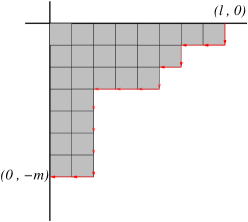
Takács observed that this probability is computable by a two-dimensional local central limit theorem, ultimately obtaining bounds on the relative error that are of order $(m+\ell)^{-3}$. These error bounds are meaningful when $n$ differs from $m\ell/2$ by up to a few multiples of $\log(m+\ell)$ standard deviations: if $\ell=\theta(m)$ this means that $|B-A/2|m^{2}=\Theta(m^{3/2}\log m)$. When $|B-A/2|\gg m^{-1/2}\log m$ the error is much bigger than the main term of the Gaussian estimate provided by the LCLT and one cannot recover meaningful information about $N_{n}(\ell,m)$. This is where Takács left off and the present manuscript picks up.

2.4 Description of our methods

We use a local large deviation computation in place of a local central limit theorem: this is possible because the restriction to an $m\times\ell$ rectangle is a linear constraint. Indeed, consider now a partition $\lambda=(\lambda_{1},\dots,\lambda_{m})$ with at most $m$ parts (so some $\lambda_{j}$ may be zero) and define $\lambda_{0}:=\ell$ and $\lambda_{m+1}:=0$. It is convenient to encode a partition with respect to its gaps $x_{j}:=\lambda_{j}-\lambda_{j+1}$, so the condition that $\lambda$ be a partition of $n$ of size at most $\ell$ is equivalent to $x_{j}\geq 0$ and

$$\sum_{j=0}^{m}x_{j}=\ell\,,\qquad\qquad\sum_{j=0}^{m}jx_{j}=n\,.$$ (7)

Figure 2 gives a pictorial proof.

Figure 2: The total area $n$ of a partition is composed of rectangles of area $jx_{j}$

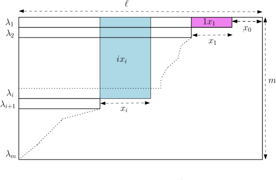
Solving the large deviation problem produces a “tilted measure” in which the gaps $X_{j}$ are no longer IID reduced geometrics with parameter $1/2$ but are instead given by independent reduced geometric variables whose parameters $q_{j}=1-p_{j}$ vary in a log-linear manner. Log-linearity is dictated by the variational large deviation problem and leads to the same simplification as before. Not all partitions have the same probability under the tilted measure, but all those resulting in a given value of $\ell$ and $n$ do have the same probability. Lastly, one must choose the particular linear function $\log q_{j}=-c-d(j/m)$ to ensure that $\lambda$ being a partition of $n$ with parts of size at most $\ell$ will again be in the central part of the tilted measure, so that asymptotics can be read off from a local CLT for the tilted measure.

The tilted measures $\mathbb{P}_{m}$ that we employ are denoted $\mu_{x,y}$ in [VY01] and referred to there as the grand ensemble of partitions. That paper, however, was not concerned with enumeration, only with limit shape results. For this reason they do not state or prove enumeration results. In fact [Pet09] is able to prove the shape result by estimating exponential rates only, showing rather elegantly that an $\varepsilon$ error in the rescaled shape leads to an exponential decrease in the number of partitions. The present manuscript combines the idea of the grand ensemble with some precise central limit estimates and some algebra inverting the relation between the log-linear parameters and the parameters $A$ and $B$ defining the respective limits of $\ell/m$ and $n/m^{2}$ to give estimates on $N_{n}(\ell,m)$ precise enough also to yield asymptotic estimates on $N_{n+1}(\ell,m)-N_{n}(\ell,m)$.

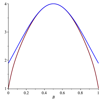
The first step of carrying this out necessarily recovers the leading exponential behavior for $N_{n}(\ell,m)$, which is implicit in [VY01] and [Pet09] though Petrov only states it as an upper bound. Interestingly, Takács did not seem to be aware of the ease with which the exponential rate may be obtained. His result states a Gaussian estimate and an error term. As noted above, it is nontrivial only when the $(m+\ell)^{-3}$ relative error term does not swamp the main terms, which occurs when $n$ is close to $\ell m/2$ (see also [AA91]). Figure 3 shows Takács’ predicted exponential growth rate on a family of examples compared to the actual exponential growth rate that follows from Theorem 1.

Figure 3: Exponential growth of $N_{Bm^{2}}(m,m)$ predicted by Takács’ formula (blue, above) compared to the actual exponential growth given by Theorem 1 (red, below).

3 A discretized analogue to Theorem 1

We now implement this program to derive asymptotics. With $c_{m}$ and $d_{m}$ to be specified later, let $q_{j}:=e^{-c_{m}-jd_{m}/m}$, let $p_{j}:=1-q_{j}$ and let

$$L_{m}:=\sum_{j=0}^{m}\log p_{j}.$$

Let $\mathbb{P}_{m}$ be a probability law making the random variables $\{X_{j}:0\leq j\leq m\}$ independent reduced geometrics with respective parameters $p_{j}$. Define random variables $S_{m}$ and $T_{m}$ by

$$S_{m}:=\sum_{i=0}^{m}X_{i}\,;\qquad T_{m}:=\sum_{i=1}^{m}iX_{i}\,,$$ (8)

corresponding to the unique partition $\lambda$ satisfying $X_{j}=\lambda_{j}-\lambda_{j+1}$. We first prove a result similar to Theorem 1, except that the parameters $c$ and $d$ that solve integral Equations (2) and (3) are replaced by $c_{m}$ and $d_{m}$ satisfying the discrete summation Equations (9) and (10) below. These equations say that $\mathbb{E}S_{m}=\ell$ and $\mathbb{E}T_{m}=m$. Writing this out, using $\displaystyle\mathbb{E}X_{j}=1/p_{j}-1=1/\left(1-e^{-c_{m}-d_{m}j/m}\right)-1$, gives

$$\ell =\sum_{j=0}^{m}\frac{1}{1-e^{-c_{m}-d_{m}j/m}}-(m+1)$$ (9)

$$n =m\sum_{j=0}^{m}\frac{j/m}{1-e^{-c_{m}-d_{m}j/m}}-\frac{m(m+1)}{2}\,.$$ (10)

Let $M_{m}$ denote the covariance matrix for $(S_{m},T_{m})$. The entries may be computed from the basic identity ${\rm Var}\,(X_{j})=q_{j}/p_{j}^{2}$, resulting in

$${\rm Var}\,(S_{m}) =\sum_{j=0}^{m}\frac{e^{-c_{m}-d_{m}j/m}}{\left(1-e^{-c_{m}-d_{m}j/m}\right)^{2}}$$ (11)

$${\rm Cov}\,(S_{m},T_{m}) =\sum_{j=0}^{m}j\frac{e^{-c_{m}-d_{m}j/m}}{\left(1-e^{-c_{m}-d_{m}j/m}\right)^{2}}$$ (12)

$${\rm Var}\,(T_{m}) =\sum_{j=0}^{m}j^{2}\frac{e^{-c_{m}-d_{m}j/m}}{\left(1-e^{-c_{m}-d_{m}j/m}\right)^{2}}\,.$$ (13)

Theorem 4 (discretized analogue).

Let $c_{m}$ and $d_{m}$ satisfy (9) – (10). Define $\alpha_{m},\beta_{m}$ and $\gamma_{n}$ to be the normalized entries of the covariance matrix

$$\alpha_{m}:=m^{-1}{\rm Var}\,(S_{m})\;;\qquad\beta_{m}:=m^{-2}{\rm Cov}\,(S_{m},T_{m})\;;\qquad\gamma_{m}:=m^{-3}{\rm Var}\,(T_{m})\;,$$

which are $O(1)$ as $m\rightarrow\infty$. Again, let $A:=\ell/m$ and $B:=n/m^{2}$ and $\Delta_{m}:=\alpha_{m}\gamma_{m}-\beta_{m}^{2}$. Then as $m\to\infty$ with $\ell$ and $n$ varying so that $(A,B)$ remains in a compact subset of $\{(x,y):x\geq 2y>0\}$,

$$N_{n}(\ell,m)\sim\frac{1}{2\pi m^{2}\sqrt{\Delta_{m}}}\exp\left\{m\left(-\frac{L_{m}}{m}+c_{m}A+d_{m}B\right)\right\}\,.$$ (14)

Proof.

The atomic probabilities $\mathbb{P}_{m}({\bf X}={\bf x})$ depend only on $S_{m}$ and $T_{m}$ as

$$\log\mathbb{P}_{m}({\bf X}={\bf x}) =\sum_{j=0}^{m}\left(\log p_{j}+x_{j}\log q_{j}\right)$$

$$=L_{m}-\sum_{j=0}^{m}\left(c_{m}+j\frac{d_{m}}{m}\right)x_{j}$$

$$=L_{m}-c_{m}\left(\sum_{j=0}^{m}x_{j}\right)-\frac{d_{m}}{m}\left(\sum_{j=0}^{m}jx_{j}\right).$$

In particular, for any ${\bf x}$ satisfying (7),

$$\log\mathbb{P}({\bf X}={\bf x})=L_{m}-c_{m}\ell-\frac{d_{m}}{m}n\,.$$ (15)

Three things are equivalent: $(i)$ the vector ${\bf X}$ satisfies the identities (7); $(ii)$ the pair $(S_{m},T_{m})$ is equal to $(\ell,n)$; $(iii)$ the partition $\lambda=(\lambda_{1},\ldots,\lambda_{m})$ defined by $\lambda_{j}-\lambda_{j+1}=X_{j}$ for $2\leq j\leq m-1$, together with $\lambda_{1}=\ell-X_{0}$ and $\lambda_{m}=X_{m}$, is a partition of $n$ fitting inside a $m\times\ell$ rectangle. Thus,

$$N_{n}(\ell,m) =\mathbb{P}_{m}\left[(S_{m},T_{m})=(\ell,n)\right]\,\exp\left(-L_{m}+c_{m}\ell+\frac{d_{m}}{m}n\right)$$

$$=\mathbb{P}_{m}\left[(S_{m},T_{m})=(\ell,n)\right]\,\exp\left[m\left(-\frac{L_{m}}{m}+c_{m}A+d_{m}B\right)\right]\,.$$ (16)

Comparing (14) to (16), the proof is completed by an application of the LCLT in Lemma 5. ∎

Lemma 5 is stated for an arbitrary sequence of parameters $p_{0},\ldots,p_{m}$ bounded away from 0 and 1, though we need it only for $p_{j}=1-e^{-c_{m}-d_{m}j/m}$. For a $2\times 2$ matrix $M$, denote by $M(s,t):=[s\,,\,\,t]\,M\,[s\,,\,\,t]^{T}$ the corresponding quadratic form.

Lemma 5 (LCLT).

Fix $0<\delta<1$ and let $p_{0},\ldots,p_{m}$ be any real numbers in the interval $[\delta,1-\delta]$. Let $\{X_{j}\}$ be independent reduced geometrics with respective parameters $\{p_{j}\}$, $S_{m}:=\sum_{j=0}^{m}X_{j},$ and $T_{m}:=\sum_{j=0}^{m}jX_{j}$. Let $M_{m}$ be the covariance matrix for $(S_{m},T_{m})$, written

$$M_{m}=\displaystyle\left(\begin{array}[]{cc}\alpha_{m}m&\beta_{m}m^{2}\\ \beta_{m}m^{2}&\gamma_{m}m^{3}\end{array}\right)\,,$$

$Q_{m}$ denote the inverse matrix to $M_{m}$, and $\Delta_{m}=m^{-4}\det M_{m}=\alpha_{m}\gamma_{m}-\beta_{m}^{2}$. Let $\mu_{m}$ and $\nu_{m}$ denote the respective means $\mathbb{E}S_{m}$ and $\mathbb{E}T_{m}$. Denote $p_{m}(a,b):=\mathbb{P}((S_{m},T_{m})=(a,b))$. Then

$$\sup_{a,b\in\mathbb{Z}}m^{2}\left|p_{m}(a,b)-\frac{1}{2\pi(\det M_{m})^{1/2}}e^{-\frac{1}{2}Q_{m}(a-\mu_{m},b-\nu_{m})}\right|\to 0$$ (17)

as $m\to\infty$, uniformly in the parameters $\{p_{j}\}$ in the allowed range. In particular, if the sequence $(a_{m},b_{m})$ satisfies $Q_{m}(a_{m}-\mu_{m},b_{m}-\nu_{m})\to 0$ then

$$\mathbb{P}(S_{m}=a_{m},T_{m}=b_{m})=\frac{1}{2\pi\sqrt{\Delta_{m}}m^{2}}\left(1+O\left(m^{-3/2}\right)\right)\,.$$

The following consequence will be used to prove Theorem 2.

Corollary 6 (LCLT consecutive differences).

Let $\mathcal{N}_{m}(a,b):=\frac{1}{2\pi(\det M_{m})^{1/2}}e^{-\frac{1}{2}Q_{m}(a-\mu_{m},b-\nu_{m})}$ be the normal approximation in Equation (17). Using the notation of Lemma 5,

$$\sup_{a,b\in\mathbb{Z}}\bigg{|}p_{m}(a,b+1)-p_{m}(a,b)-\big{(}\mathcal{N}_{m}(a,b+1)-\mathcal{N}_{m}(a,b)\big{)}\bigg{|}=O(m^{-4}).$$

The technical but unsurprising proofs of Lemma 5 and Corollary 6 are given in the Appendix at the end of this article.

4 Limit shape

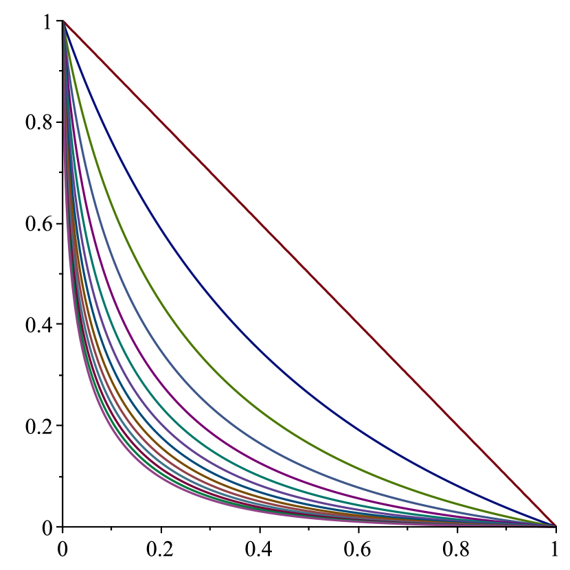
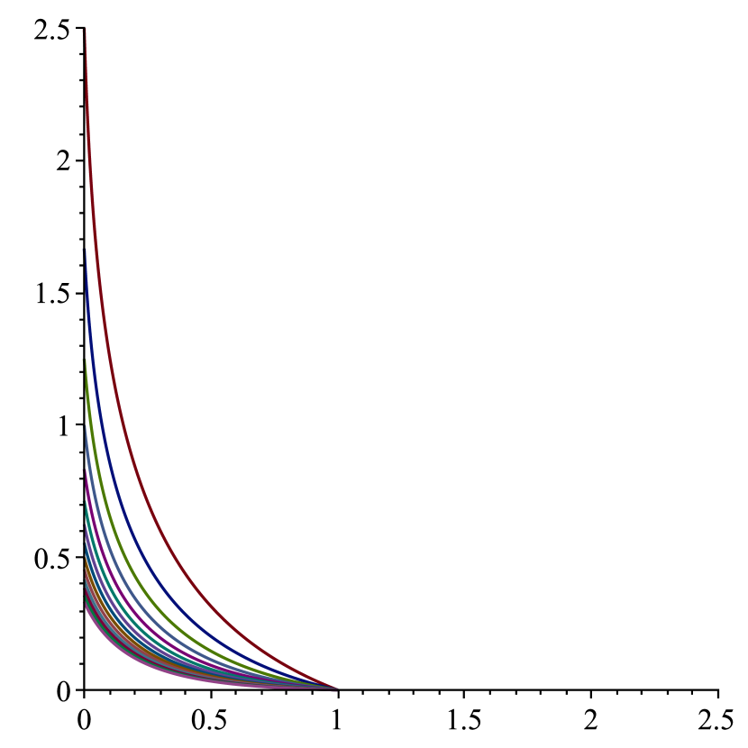
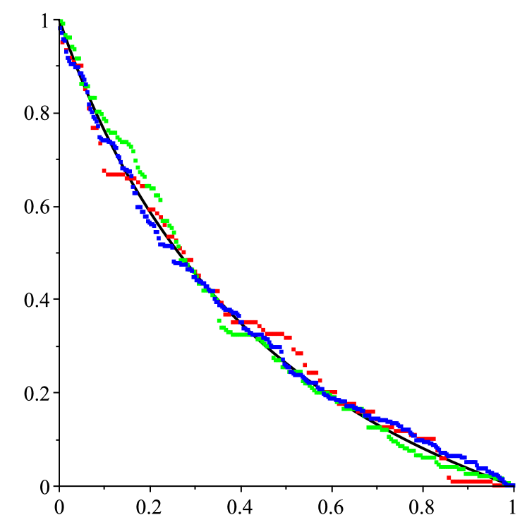
Suppose a Young diagram is chosen uniformly from among all partitions of $n$ fitting in a $m\times\ell$ rectangle. To simplify calculations, we imagine this Young diagram outlining a compact set in the fourth quadrant of the plane and rotate $90^{\circ}$ counterclockwise to obtain a shape in the first quadrant. Let $\Xi_{n,m,\ell}$ denote the random set obtained in this manner after rescaling by a factor of $1/m$, so that the length in the positive $x$-direction is bounded by 1. Fix $A>2B>0$ and metrize compact sets of $\mathbb{R}^{2}$ by the Hausdorff metric. As $m\to\infty$ with $\ell/m\to A$ and $n/m^{2}\to B$, the random set $\Xi_{n,m,\ell}$ converges in distribution to a deterministic set $\Xi^{A,B}$. See Figure 4 for some examples.

Our methods immediately recover the distributional convergence result $\Xi_{n,m,\ell}\to\Xi^{A,B}$. As previously mentioned, this limit shape was known to Petrov [Pet09] and others. Petrov identifies it as a portion of the limit curve for unrestricted partitions, which itself was posed as a problem by Vershik and answered in [ST77a, ST77b] (see also [Ver96]). Because this result is already known, along with precise fluctuation information which we do not derive, we give only the short argument here for distributional convergence. We do not determine the best possible fluctuation results following from this method.

The shape $\Xi_{n,m,\ell}$ is determined by its boundary, a polygonal path obtained from a partition $\lambda$ by filling in unit vertical connecting lines in the step function $x\mapsto m^{-1}\lambda_{\lfloor mx\rfloor}$. Recall that the probability measure $\mathbb{P}_{m}$ restricted to the event $\{(S_{m},T_{m})=(\ell,n)\}$ gives all partitions counted by $N_{n}(m,\ell)$ equal probability and that $\mathbb{P}_{m}$ gives the event $\{(S_{m},T_{m})=(\ell,n)\}$ probability $\Theta(m^{-2})$. Distributional convergence of $\Xi_{n,m,\ell}$ to $\Xi^{A,B}$ then follows from the following.

Proposition 7.

Fix $A>2B>0$. Define the maximum discrepancy by

$$\mathcal{M}:=\max_{0\leq j\leq m}\left|\sum_{i=0}^{j}\left(X_{i}-\frac{q_{i}}{p_{i}}\right)\right|\,.$$

Then for any $\varepsilon>0$,

$$\mathbb{P}_{m}\left[\mathcal{M}\geq\varepsilon m\right]=o(m^{-2})$$

as $m\to\infty$ with $\ell/m\to A$ and $n/m\to B$.

Proof.

This is a routine application of exponential moment bounds. By our definition of $p_{i}$, in this regime there exists $\delta>0$ such that $p_{i}\in[\delta,1-\delta]$ for all $i$. Therefore, there are $\eta,K>0$ such that for $\lambda<\eta$, the mean zero variables $X_{i}-q_{i}/p_{i}$ all satisfy $\mathbb{E}\exp(\lambda(X_{i}-q_{i}/p_{i}))\leq\exp(K\lambda^{2})$. Independence of the family $\{X_{i}\}$ then gives

$$\mathbb{E}\exp\left[\lambda\sum_{i=0}^{j}(X_{i}-p_{i}/q_{i})\right]\leq e^{Km\lambda^{2}}$$

for all $j\leq m$. By Markov’s inequality,

$$\mathbb{P}(|X_{i}-p_{i}/q_{i}|\geq\varepsilon m)\leq e^{Km\lambda^{2}-\lambda m}\,.$$

Fixing $\lambda=1/(2K)$ shows that this probability is bounded above by $\exp(-m/(4K))$. Hence, $\mathbb{P}(\mathcal{M}\geq\varepsilon m)\leq me^{-m/(4K)}=o(m^{-2})$ as desired. ∎

To see that Proposition 7 implies the limit shape statement, let $\lambda_{i}:=\ell-(X_{0}+\cdots+X_{i-1})$ so that

$$y^{(m)}(i):=\mathbb{E}_{m}\lambda_{i}=\ell-\sum_{j=0}^{i-1}q_{j}/p_{j}.$$

Proposition 7 shows the boundary of $\Xi_{m}$ to be within $o(m)$ of the step function $y^{(m)}(\cdot)$ except with probability $o(m^{-2})$. Since $\mathbb{P}_{m}$ restricted to the event $\{(S_{m},T_{m})=(\ell,n)\}$ gives all partitions counted by $N_{n}(m,\ell)$ equal probability and $\mathbb{P}_{m}$ gives the event $\{(S_{m},T_{m})=(\ell,n)\}$ probability $\Theta(m^{-2})$, the conditional law $(\mathbb{P}_{m}\,|\,(S_{m},T_{m})=(\ell,n))$ gives the event $\{\mathcal{M}>\varepsilon m\}$ probability $o(1)$ as $m\to\infty$ with $\ell/m\to A$ and $n/m\to B$. Thus, the boundary of $\Xi_{m}$ converges in distribution to the limit

$$y(x):=\lim_{m\to\infty}m^{-1}y^{(m)}(\lfloor mx\rfloor)\,.$$ (18)

Figure 4 shows examples of two families of the limit curve as well as a plot of the limit curve against uniformly generated restricted partitions for several values of $m$ in the range $[120,300]$.

(a) $(A,B)=(1,1/k)$
$k=2,\dots,15$

(b) $(A,B)=(5/k,1/k)$
$k=2,\dots,15$

(c) Limit curve of $(A,B)=(1,1/3)$ and random partitions of size 120, 201 and 300.

Figure 4: Limit shapes of scaled partitions as $m\rightarrow\infty$.

Substituting the definition of $y^{(m)}(i)$ into (18) and evaluating the limit as an integral gives

$$y(x)=A+x-\int_{0}^{x}\frac{1}{1-e^{-c-dt}}dt=A+x-\frac{1}{d}\ln\left(\frac{e^{xd+c}-1}{e^{c}-1}\right)\,.$$

After expressing $c$ in terms of $d$, this may be written implicitly as

$$e^{(A+1)d}-1=(e^{d}-1)e^{d(A-y)}+(e^{Ad}-1)e^{d(1-x)}$$

which simplifies to

$$(1-e^{-c})e^{d(A-y)}+e^{-c}e^{-dx}=1$$ (19)

as long as $A>2B$; in the special case $A=2B$ one obtains simply $y=A\cdot(1-x)$.

It is worth comparing this result with the limit shape derived in [Pet09]. There the limit shape of the boxed partitions is identified as the portion of the curve $\{e^{-x}+e^{-y}=1\}$, which is the limit shape of unrestricted partitions. The portion is determined implicitly by the restriction that the endpoints of the curve are the opposite corners of a $1\times A$-proportional rectangle and that the area under the curve has the desired proportion, that is $B/A$ of the total rectangular area. To see that this matches (19) we can calculate the given portion explicitly.

Let $x=s_{1},s_{2}$ be the starting and ending points of the bounding rectangle. The side ratio and the area requirement are respectively equivalent to

$$\frac{\log(1-e^{s_{1}})-\log(1-e^{-s_{2}})}{s_{2}-s_{1}} =A$$

and

$$\int_{s_{1}}^{s_{2}}-\log(1-e^{-t})dt+(s_{2}-s_{1})\log(1-e^{-s_{2}}) =B(s_{2}-s_{1})^{2}$$

which simplify to

$$A = \frac{1}{s_{2}-s_{1}}\log\left(\frac{e^{s_{2}}-1}{e^{s_{2}}-e^{s_{2}-s_{1}}}\right)\,,$$ (20)

$$B = \frac{-{\rm dilog}\,(1-e^{-s_{2}})+{\rm dilog}\,(1-e^{-s_{1}})+(s_{2}-s_{1})\log(1-e^{-s_{2}})}{(s_{2}-s_{1})^{2}}\,.$$ (21)

Comparing these equations with equations (2) and (3) it is immediate that the solutions are given by $s_{1}=c$ and $s_{2}=c+d$. Finally, to match the curve in the second line of equation (19) we need the coordinate transform from the curve $\gamma$ in the segment $x=[c,c+d]$ given by

$$x\to x_{1}=\frac{(x-c)}{d},\qquad y\to y_{1}-A=\frac{y+\log(1-e^{-c})}{d}$$

whence $x=dx_{1}+c$ and $y=-d(A-y_{1})-\log(1-e^{-c})$ and the curves match.

5 Existence and Uniqueness of $c,d$

We now show that for any $A\geq 2B>0$ there exists unique positive constants $c$ and $d$ satisfying Equations (2) and (3). If $A=B/2$ then $d=0$ and $c$ can be determined uniquely, so we may assume $A>2B>0$. The following lemma will be used to show uniqueness.

Lemma 8.

Let $\psi$ denote the map taking the pair $(c,d)$ to $(A,B)$ defined by the two integrals in Equations (2) and (3), and let $K$ be a compact subset of $\{(x,y):x>2y>0\}$. The Jacobian matrix $J:=D[\psi]$ is negative definite for all $(c,d)\in(0,\infty)^{2}$, and all entries of $\psi$ and $J$ (respectively $\psi^{-1}$ and $J^{-1}$) are Lipshitz continuous on $\psi^{-1}[K]$ (respectively $K$).

Proof.

Differentiating under the integral sign shows that the partial derivatives comprising the entries of $D[\psi]$ are given by

$$J_{A,c} = \int_{0}^{1}\frac{-e^{-(c+dt)}}{(1-e^{-(c+dt)})^{2}}\,dt$$

$$J_{A,d} = \int_{0}^{1}\frac{-t\,e^{-(c+dt)}}{(1-e^{-(c+dt)})^{2}}\,dt$$

$$J_{B,c} = \int_{0}^{1}\frac{-t\,e^{-(c+dt)}}{(1-e^{-(c+dt)})^{2}}\,dt$$

$$J_{B,d} = \int_{0}^{1}\frac{-t^{2}\,e^{-(c+dt)}}{(1-e^{-(c+dt)})^{2}}\,dt\,;$$

note that each term is negative. Let $\rho$ denote the finite measure on $[0,1]$ with density $e^{-(c+dt)}/(1-e^{-(c+dt)})^{2}$ and let $\mathbb{E}_{\rho}$ denote expectation with respect to $\rho$. Then

$$J_{A,c}=\mathbb{E}_{\rho}[-1],\qquad J_{A,d}=J_{B,c}=\mathbb{E}_{\rho}[-t],\qquad J_{B,d}=\mathbb{E}_{\rho}[-t^{2}],$$

and

$$\det J=\mathbb{E}_{\rho}[1]\cdot\mathbb{E}_{\rho}[t^{2}]-\left(\mathbb{E}_{\rho}[t]\right)^{2}=\mathbb{E}_{\rho}[1]^{2}\cdot{\rm Var}\,_{\sigma}[t],$$

where ${\rm Var}\,_{\sigma}[t]$ denotes the variance of $t$ with respect to the normalized measure $\sigma=\rho/\mathbb{E}_{\rho}[1]$. In particular, $\det J$ is positive, and bounded above and below when $c$ and $d$ are bounded away from 0, implying the stated results on Lipshitz continuity. As $J$ is real and symmetric, it has real eigenvalues. Since the trace of $J$ is negative while its determinant is positive, the eigenvalues of $J$ have negative sum and positive product, meaning both are strictly negative and $J$ is negative definite for any $c,d>0$. ∎

Lemma 9.

For any $A>0$ and $B\in(0,A/2)$ there exist unique $c,d>0$ satisfying Equations (2) and (3). Moreover, for a fixed $A$, when $B$ decreases from $A/2$ to $0$ then $d$ increases strictly from $0$ to $\infty$ and $c$ decreases strictly from $\log\left(\frac{A+1}{A}\right)$ to $1$. When $B>0$ is fixed and $A$ goes to $\infty$ then $c$ goes to $0$ and $d$ goes to the root of

$$d^{2}=B\left(d\log(1-e^{-d})-{\rm dilog}\,(1-e^{-d})\right).$$

Proof.

Solving Equation (2) for $c$ (assuming $d\geq 0$) gives

$$c=\log\left(\frac{e^{(A+1)d}-1}{e^{(A+1)d}-e^{d}}\right).$$

Substituting this into Equation (3) gives an explicit expression for $B$ in terms of $A$ and $d$, and shows that for fixed $A>0$ as $d$ goes from 0 to infinity $B$ goes from $A/2$ to 0. By continuity, this implies the existence of the desired $c$ and $d$. It also shows that, for a fixed $A$, $c$ is a decreasing function of $d$ with the given maximal and minimal values as $d$ goes from $0$ to $\infty$.

To prove uniqueness, we note that for ${\bf x},{\bf y}\in\mathbb{R}^{2}$ Stokes’ theorem implies

$$\psi({\bf y})-\psi({\bf x})=\int_{0}^{1}D[\psi]\left(t{\bf x}+(1-t){\bf y}\right)\cdot({\bf x}-{\bf y})\,dt$$

so that

$$({\bf x}-{\bf y})^{T}\cdot\left(\psi({\bf y})-\psi({\bf x})\right)=\int_{0}^{1}\left[({\bf x}-{\bf y})^{T}\cdot D[\psi]\left(t{\bf x}+(1-t){\bf y}\right)\cdot({\bf x}-{\bf y})\right]dt.$$

When ${\bf x}\neq{\bf y}$, negative-definiteness of $D[\psi]$ implies that the last integrand is strictly negative on $[0,1]$, and $\psi({\bf y})\neq\psi({\bf x})$. Thus, distinct values of $c$ and $d$ give distinct values of $A$ and $B$.

To see the monotonicity, let $A$ be fixed and let $F_{B}(d)=B$ be the equation obtained after substituting $c=c(A,d)$ above in Equation (3), i.e. $F_{B}(d)=\psi_{2}(c(A,d),d)$. Then $d$ is a decreasing function of $B$ and vice versa since

$$\frac{\partial F_{B}(d)}{\partial d}=\frac{J_{B,d}J_{A,c}-J_{A,d}J_{B,c}}{J_{A,c}}=\frac{\det D[\psi]}{J_{A,c}}<0\,.$$

For the last part, the explicit formula for $c$ in terms of $A$ and $d$ shows that $c\to 0$. Substitution in Equation (3) gives the desired equation.

∎

6 Proof of Theorem 1 from the discretized result

Here we show how $c_{m}$ and $d_{m}$ from the discretized result are related to $c,d$ defined independently of $m$. The proof below also shows that $c_{m}$ and $d_{m}$ exist and are unique.

The Euler-MacLaurin summation formula [dB58, Section 3.6] gives an expansion

$$\frac{L_{m}}{m} =\int_{0}^{1}\log(1-e^{-c_{m}-d_{m}t})\,dt+\frac{\log(1-e^{-c_{m}})+\log(1-e^{-c_{m}-d_{m}})}{2m}+O(m^{-2})$$

$$=\frac{{\rm dilog}\,(1-e^{-c_{m}-d_{m}})-{\rm dilog}\,(1-e^{-c_{m}})}{d_{m}}+\frac{\log(1-e^{-c_{m}})+\log(1-e^{-c_{m}-d_{m}})}{2m}+O(m^{-2})$$ (22)

of the sum $L_{m}$ in terms of $c_{m}$ and $d_{m}$. Assume that there is an asymptotic expansion

$$c_{m} = c+um^{-1}+O(m^{-2})$$ (23)

$$d_{m} = d+vm^{-1}+O(m^{-2})$$ (24)

as $m\rightarrow\infty$, where $u$ and $v$ are constants depending only on $A$ and $B$. Under such an assumption, substitution of Equations (23) and (24) into Equation (22) implies

$$\frac{L_{m}}{m} =\frac{{\rm dilog}\,(1-e^{-c-d})-{\rm dilog}\,(1-e^{-c})}{d}+\frac{uA+vB}{m}+O(m^{-2})$$

$$=\log(1-e^{-c-d})-dB+\frac{uA+vB}{m}+O(m^{-2}).$$ (25)

Substituting Equations (23)–(6) into Equation (14) of Theorem 4 and taking the limit as $m\rightarrow\infty$ then gives Theorem 1, as

$$\Delta_{m}\rightarrow\left(\int_{0}^{1}\frac{e^{-c-dt}}{(1-e^{-c-dt})^{2}}\,dt\right)\left(\int_{0}^{1}\frac{t^{2}e^{-c-dt}}{(1-e^{-c-dt})^{2}}\,dt\right)-\left(\int_{0}^{1}\frac{te^{-c-dt}}{(1-e^{-c-dt})^{2}}\,dt\right)^{2}=\Delta.$$

It remains to show the expansions in Equations (23) and (24). For $x,y>0$, define

$${\overline{S}}_{m}(x,y) :=\frac{1}{m}\sum_{j=0}^{m}\frac{1}{1-e^{-(x+yj/m)}}-1\,,$$

$${\overline{T}}_{m}(x,y) :=\frac{1}{m}\sum_{j=0}^{m}\frac{j/m}{1-e^{-(x+yj/m)}}-\frac{1}{2}\,.$$

Another application of the Euler-MacLaurin summation formula implies

$${\overline{S}}_{m}(c,d) =A+A_{1}(c,d)m^{-1}+O(m^{-2})\,,$$ (26)

$${\overline{T}}_{m}(c,d) =B+B_{1}(c,d)m^{-1}+O(m^{-2})\,,$$ (27)

with

$$A_{1}=\frac{1}{2}\left(\frac{1}{1-e^{-c}}+\frac{1}{1-e^{-c-d}}\right)\qquad\text{and}\qquad B_{1}=\frac{1}{2(1-e^{-c-d})}.$$

Let $\mathcal{J}$ denote the Jacobian $D[\psi]$ of the map $\psi$, introduced in Lemma 8, with respect to $c$ and $d$, and let

$$(c_{m}^{\prime},d_{m}^{\prime})=(c,d)-m^{-1}\mathcal{J}^{-1}\cdot(A_{1}-1,B_{1}-1/2)^{T}.$$

A Taylor expansion around the point $(c,d)$ gives

$$\begin{pmatrix}{\overline{S}}_{m}(c_{m}^{\prime},d_{m}^{\prime})\\ {\overline{T}}_{m}(c_{m}^{\prime},d_{m}^{\prime})\end{pmatrix} =\begin{pmatrix}{\overline{S}}_{m}(c,d)\\ {\overline{T}}_{m}(c,d)\end{pmatrix}-\left(\mathcal{J}+O\left(m^{-1}\right)\right)\cdot\left(m^{-1}\mathcal{J}^{-1}\begin{pmatrix}A_{1}\\ B_{1}\end{pmatrix}\right)+O(m^{-2})$$

$$=\begin{pmatrix}A-1/m\\ B-1/2m\end{pmatrix}+O\left(m^{-2}\right)$$

$$=\begin{pmatrix}{\overline{S}}_{m}(c_{m},d_{m})\\ {\overline{T}}_{m}(c_{m},d_{m})\end{pmatrix}+O\left(m^{-2}\right),$$

where Equations (26) and (27) were used to approximate the Jacobian of $\psi_{m}:(x,y)\mapsto\left({\overline{S}}_{m}(x,y),{\overline{T}}_{m}(x,y)\right)$ with respect to $x$ and $y$.

The map $\psi_{m}$ is Lipschitz for a similar reason as its continuous analogue. Namely, consider the partial derivatives

$$J_{S,x} = \frac{1}{m}\sum_{j=0}^{m}\ -\frac{e^{-x-yj/m}}{(1-e^{-x-yj/m})^{2}}\,$$

$$J_{S,y} = \frac{1}{m^{2}}\sum_{j=0}^{m}\ -\frac{j\ e^{-x-yj/m}}{(1-e^{-x-yj/m})^{2}}\,$$

$$J_{T,x} = \frac{1}{m^{2}}\sum_{j=0}^{m}\ -\frac{j\ e^{-x-yj/m}}{(1-e^{-x-yj/m})^{2}}\,$$

$$J_{S,y} = \frac{1}{m^{3}}\sum_{j=0}^{m}\ -\frac{j^{2}\ e^{-x-yj/m}}{(1-e^{-x-yj/m})^{2}}.$$

Let $\rho_{m}$ be a discrete finite measure on $R_{m}:=\{0,1/m,2/m,\ldots,1\}$ with density $e^{-x-yt}/(1-e^{-x-yt})$ for $t\in R_{m}$ and 0 otherwise, and let $\mathbb{E}_{\rho_{m}}$ be the expectation with respect to $\rho_{m}$. Then

$$J_{S,x}=\mathbb{E}_{\rho_{m}}[-1]\,,\qquad J_{T,x}=J_{S,y}=\mathbb{E}_{\rho_{m}}[-t]\,,\qquad J_{T,y}=\mathbb{E}_{\rho_{m}}[-t^{2}]$$

and

$$\det D[\psi_{m}]=\mathbb{E}_{\rho_{m}}[1]\mathbb{E}_{\rho_{m}}[t^{2}]-\mathbb{E}_{\rho_{m}}[t]^{2}=\mathbb{E}_{\rho_{m}}[1]^{2}{\rm Var}\,_{\sigma_{m}}[t]\,,$$

where $\sigma_{m}$ is the probability function $\rho_{m}/\mathbb{E}_{\rho_{m}}[1]$. For any fixed $m$ and $(x,y)$ in a compact neighborhood of $(A,B)$, both the variance and the expectation are finite and bounded away from 0, as is the Jacobian determinant. Moreover, the trace ${\rm Tr}D[\psi]=-\mathbb{E}_{\rho_{m}}[1+t^{2}]$ is bounded away from 0 and infinity, so the Jacobian is negative definite with locally bounded eigenvalues, and hence $\psi_{m}$ is locally Lipschitz. Since the norm of the Jacobian is bounded away from 0 and infinity, we have that the inverse map $\psi_{m}^{-1}$ is also locally Lipschitz in a neighborhood of $\psi^{-1}(A,B)$. Moreover, similarly to proof of existence and uniqueness of $c$ and $d$ in Section 5, we have that there indeed are $c_{m}$ and $d_{m}$ as unique solutions of Equations (9) and (10) since the Jacobian is negative semi-definite.

The trapezoid formula implies $\left|J_{S,c}-J_{A,c}\right|=O(m^{-1})$, and similar bounds for the other differences of partial derivatives in the continuous and discrete settings. Hence, the bounds for the norms and eigenvalues of $D[\psi_{m}]$ are within $O(m^{-1})$ of the ones for $D[\psi]$, and $\psi_{m}$ (and its inverse) is Lipschitz with a constant independent of $m$. Thus,

$$O(m^{-2})=\|\psi_{m}(c^{\prime}_{m},d^{\prime}_{m})-\psi_{m}(c_{m},d_{m})\|\geq C^{-1}\|(c_{m}^{\prime}-c_{m},d^{\prime}_{m}-d_{m})\|$$

for some constant $C$, so that the expansions (23) and (24) hold. $\hfill\Box$

7 Proof of Theorem 2

We will prove Theorem 2 from Equation (16) and Corollary 6. Let $p_{m}(\ell,n)=\mathbb{P}_{m}\left[(S_{m},T_{m})=(\ell,n)\right]$ and let

$$L_{m}(x,y) :=\sum_{j=0}^{m}\log(1-e^{-x-yj/m})\ ,$$ (28)

$$A_{m}(x,y) :=\sum_{j=0}^{m}\frac{1}{1-e^{-x-yj/m}}-(m+1)\ ,$$ (29)

$$B_{m}(x,y) :=\sum_{j=0}^{m}\frac{j/m}{1-e^{-x-yj/m}}-\frac{m+1}{2}\ .$$ (30)

Then $c_{m}$ and $d_{m}$ are the solutions to

$$A_{m}(c_{m},d_{m})=\ell=Am\,,\qquad B_{m}(c_{m},d_{m})=n/m=Bm\,.$$

Let $c^{\prime}_{m},d^{\prime}_{m}$ be the solutions to $A_{m}(c^{\prime}_{m},d^{\prime}_{m})=\ell$ and $B_{m}(c^{\prime}_{m},d^{\prime}_{m})=(n+1)/m$, and let $\Delta x=c^{\prime}_{m}-c_{m}=O(m^{-2})$ and $\Delta y=d^{\prime}_{m}-d_{m}=O(m^{-2})$ by the Lipschitz properties proven in Section 5. Observe that

$$\frac{\partial L_{m}(x,y)}{\partial x}=A_{m}(x,y)\quad\text{and}\quad\frac{\partial L_{m}(x,y)}{\partial y}=B_{m}(x,y).$$ (31)

Using the Taylor expansion for $L_{m}(c^{\prime}_{m},d^{\prime}_{m})$ around $(c_{m},d_{m})$ and the $L_{m}$ partial derivatives from Equation (31),

$$-L_{m}(c_{m}^{\prime},d_{m}^{\prime})=-L_{m}(c_{m}+\Delta x,d_{m}+\Delta y)=-L_{m}(c_{m},d_{m})-\Delta x\,A_{m}(c_{m},d_{m})-\Delta y\,B_{m}(c_{m},d_{y})+O(m^{-3}),$$

so that

$$-L_{m}(c_{m}^{\prime},d_{m}^{\prime})+(c_{m}+\Delta x)\ell+(d_{m}+\Delta y)(n+1)\,m^{-1}=-L_{m}(c_{m},d_{m})+c_{m}\ell+d_{m}(n+1)\,m^{-1}+O(m^{-3}).$$

To lighten notation, we now write $L_{m}:=L_{m}(c_{m},d_{m})$ and $L_{m}^{\prime}:=L_{m}(c_{m}^{\prime},d_{m}^{\prime})$. Then

$$N_{n+1}(\ell,m)-N_{n}(\ell,m) =p_{m}(\ell,n+1)\exp\left[-L_{m}^{\prime}+c_{m}^{\prime}\ell+\frac{d_{m}^{\prime}}{m}(n+1)\right]-p_{m}(\ell,n)\exp\left[-L_{m}+c_{m}\ell+\frac{d_{m}}{m}n\right]$$

$$=p_{m}(\ell,n)\exp\left[-L_{m}+c_{m}\ell+\frac{d_{m}}{m}n\right]\left[e^{d_{m}/m}-1\right]$$ (32)

$$\quad+\,\left[p_{m}(\ell,n+1)-p_{m}(\ell,n)\right]\exp\left[-L_{m}+c_{m}\ell+\frac{d_{m}}{m}(n+1)\right]$$ (33)

$$\quad+\,p_{m}(\ell,n+1)\left(e^{-L_{m}^{\prime}+c_{m}^{\prime}\ell+d_{m}^{\prime}(n+1)/m}-e^{-L_{m}+c_{m}\ell+d_{m}(n+1)/m}\right).$$ (34)

We now bound each of these summands.

• Since $d_{m}=d+O(m^{-1})$, Equation (16) implies that the quantity on line (32) equals

  $$N_{n}(\ell,m)\left(\frac{d}{m}+O(m^{-2})\right)$$

  as long as $d\notin O(m^{-1})$. This holds when $|A-B/2|\notin O(m^{-1})$ as $d=0$ when $A=B/2$ and the map taking $(A,B)$ to $(c,d)$ is Lipschitz.

• By Corollary 6,

  $$\left[p_{m}(\ell,n+1)-p_{m}(\ell,n)\right] \leq\left|\mathcal{N}_{m}(\ell,n+1)-\mathcal{N}_{m}(\ell,n)\right|+O(m^{-4})$$

  $$=O\left(m^{-2}\cdot\left|1-e^{\frac{1}{2}Q_{m}(0,1)}\right|\right)+O(m^{-4})$$

  $$=O(m^{-4}),$$

  where $Q_{m}$ is the inverse of the covariance matrix of $(S_{m},T_{m})$. Thus, the quantity on line (33) is $O(m^{-4}\cdot m^{2}N_{n}(\ell,m))=O(m^{-2}N_{n}(\ell,m))$.

• Let

  $$\psi_{m}:=\exp\bigg{[}-L_{m}^{\prime}+c_{m}^{\prime}\ell+d_{m}^{\prime}(n+1)\,m^{-1}-\left(-L_{m}+c_{m}\ell+d_{m}(n+1)\,m^{-1}\right)\bigg{]}-1=O(m^{-3}).$$

  As $p_{m}(\ell,n+1)=p_{m}(\ell,n)+O(m^{-4})$, it follows that the quantity on line (34) is

  $$p_{m}(\ell,n+1)\,e^{-L_{m}+c_{m}\ell+d_{m}(n+1)/m}\,\psi_{m} =N_{n}(\ell,m)\,\psi_{m}\,e^{d_{m}/m}+O(m^{-4}\,e^{d_{m}/m}\,e^{-L_{m}+c_{m}\ell+d_{m}n/m}\,\psi_{m})$$

  $$=O(m^{-3}N_{n}(\ell,m)).$$

Putting everything together,

$$N_{n+1}(\ell,m)-N_{n}(\ell,m)=N_{n}(\ell,m)\left(\frac{d}{m}+O(m^{-2})\right),$$

as desired. $\hfill\Box$

Appendix: Proof of the Local Central Limit Theorem

Throughout this section, $1/2\geq\delta>0$ is fixed and $\{p_{j}:0\leq j\leq m\}$ are arbitrary numbers in $[\delta,1-\delta]$. The variables $\{X_{j}\}$ and $(S_{m},T_{m})$ are as in Lemma 5; we drop the index $m$ on the remaining quantities $\alpha_{m},\beta_{m},\gamma_{m},\Delta_{m},\mu_{m},\nu_{m},p_{m}(a,b)$ and the matrices $M_{m}$ and $Q_{m}$. Recall the quadratic form notation $M(s,t):=[s\,,\,\,t]\,M\,[s\,,\,\,t]^{T}$.

Lemma 10.

The constants $\alpha,\beta,\gamma$ and $\Delta$ are bounded below and above by positive constants depending only on $\delta$.

Proof: Upper and lower bounds on $\alpha,\beta$ and $\gamma$ are elementary: $\displaystyle\alpha\in\left[\frac{\delta}{(1-\delta)^{2}},\frac{(1-\delta)}{\delta^{2}}\right],\beta\in\left[\frac{\delta}{2(1-\delta)^{2}},\frac{(1-\delta)}{2\delta^{2}}\right]$ and $\displaystyle\gamma\in\left[\frac{\delta}{3(1-\delta)^{2}},\frac{(1-\delta)}{3\delta^{2}}\right]$. The upper bound on $\Delta$ follows from these.

For the lower bound on $\Delta$, let $\displaystyle{\tilde{M}}=\left(\begin{array}[]{cc}\alpha_{n}&\beta_{n}\\ \beta_{n}&\gamma_{n}\end{array}\right)$ denote $M$ without the factors of $m$. We show $\Delta$ is bounded from below by the positive constant $(4-\sqrt{13})\delta/6$. A lower bound for the determinant $\Delta$ of $\tilde{M}$ is $|\lambda|^{2}$ where $\lambda$ is the least modulus eigenvalue of $\tilde{M}$; note that $|\lambda|^{2}=\inf_{\theta}\tilde{M}(\cos\theta,\sin\theta)$. We compute

$$\tilde{M}(\cos\theta,\sin\theta) =m^{-1}\mathbb{E}\left(\cos\theta S+m^{-1}\sin\theta T\right)^{2}$$

$$\geq\delta m^{-1}\sum_{k=0}^{m}\left(\cos\theta+\frac{k}{m}\sin\theta\right)^{2}$$

$$>\delta\cdot\left(\cos^{2}\theta+\cos\theta\sin\theta+\frac{1}{3}\sin^{2}\theta\right)\,.$$

This is at least $\displaystyle\frac{4-\sqrt{13}}{6}\delta$ for all $\theta$, proving the lemma. $\hfill\Box$

Lemma 11.

Let $X_{p}$ denote a reduced geometric with parameter $p$. For every $\delta\in(0,1/2)$ there is a $K$ such that simultaneously for all $p\in[\delta,1-\delta]$,

$$\left|\log\mathbb{E}\exp(i\lambda X_{p})-\left(i\frac{q}{p}\lambda-\frac{q^{2}}{2p^{2}}\lambda^{2}\right)\right|\leq K\lambda^{3}\,.$$

Proof: For fixed $p$ this is Taylor’s remainder theorem together with the fact that the characteristic function $\phi_{p}(\lambda)$ of $X_{p}$ is thrice differentiable. The constant $K(p)$ one obtains this way is continuous in $p$ on the interval $(0,1)$, therefore bounded on any compact sub-interval. $\hfill\Box$

Proof of the LCLT: The proof of Lemma 5 comes from expressing the probability as an integral of the characteristic function, via the inversion formula, and then estimating the integrand in various regions.

Let $\phi(s,t):=\mathbb{E}e^{i(sS+tT)}$ denote the characteristic function of $(S,T)$. Centering the variables at their means, denote $\widehat{S}:=S-\mu$, $\widehat{T}:=T-\nu$, and $\widehat{\phi}(s,t):=\mathbb{E}e^{i(s\widehat{S}+t\widehat{T})}$ so that $\phi(s,t)=\widehat{\phi}(s,t)e^{is\mu+it\nu}$. Then

$$p(a,b) =\frac{1}{(2\pi)^{2}}\int_{-\pi}^{\pi}\int_{-\pi}^{\pi}e^{-isa-itb}\phi(s,t)\,ds\,dt$$

$$=\frac{1}{(2\pi)^{2}}\int_{-\pi}^{\pi}\int_{-\pi}^{\pi}e^{-is(a-\mu)-it(b-\mu)}{\widehat{\phi}}(s,t)\,ds\,dt\,.$$ (35)

Following the proof of the univariate LCLT for IID variables found in [Dur10], we observe that

$$\frac{1}{2\pi(\det M)^{1/2}}e^{-\frac{1}{2}Q(a-\mu,b-\nu)}=\frac{1}{(2\pi)^{2}}\int_{-\infty}^{\infty}\int_{-\infty}^{\infty}e^{-is(a-u)-it(b-v)}\exp\left(-\frac{1}{2}M(s,t)\right)\,ds\,dt\,.$$ (36)

Hence, comparing this to (35) and observing that $e^{-is(a-\mu)-it(b-\nu)}$ has unit modulus, the absolute difference between $p(a,b)$ and the left-hand side of (36) is bounded above by

$$\frac{1}{(2\pi)^{2}}\int_{-\infty}^{\infty}\int_{-\infty}^{\infty}\left|{\bf 1}_{(s,t)\in[-\pi,\pi]^{2}}\widehat{\phi}(s,t)-e^{-(1/2)M(s,t)}\right|ds\,dt\,.$$ (37)

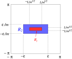
Fix positive constants $L$ and $\varepsilon$ to be specified later and decompose the region ${\mathcal{R}}:=[-\pi,\pi]^{2}$ as the disjoint union ${\mathcal{R}}_{1}+{\mathcal{R}}_{2}+{\mathcal{R}}_{3}$, where

$${\mathcal{R}}_{1} =[-Lm^{-1/2},Lm^{-1/2}]\times[-Lm^{-3/2},Lm^{-3/2}]$$

$${\mathcal{R}}_{2} =[-\varepsilon,\varepsilon]\times[-\varepsilon m^{-1},\varepsilon m^{-1}]\;\;\setminus\;{\mathcal{R}}_{1}$$

$${\mathcal{R}}_{3} ={\mathcal{R}}\setminus({\mathcal{R}}_{1}\cup{\mathcal{R}}_{2})\,;$$

see Figure 5 for details.

Figure 5: The regions ${\mathcal{R}}_{1}\subseteq{\mathcal{R}}_{2}\subseteq{\mathcal{R}}$ in the proof of the LCLT.

As $\int_{{\mathcal{R}}_{2}^{c}}e^{-(1/2)M(s,t)}\,ds\,dt$ decays exponentially with $m$, it suffices to obtain the following estimates

$$\int_{{\mathcal{R}}_{1}}\left|{\widehat{\phi}}(s,t)-e^{-(1/2)M(s,t)}\right|\,ds\,dt =O\left(m^{-5/2}\right)$$ (38)

$$\int_{{\mathcal{R}}_{2}}\left|{\widehat{\phi}}(s,t)-e^{-(1/2)M(s,t)}\right|\,ds\,dt =O(m^{-5/2})$$ (39)

$$\int_{{\mathcal{R}}_{3}}\left|{\widehat{\phi}}(s,t)\right|\,ds\,dt =o\left(m^{-3}\right).$$ (40)

By independence of $\{X_{j}\}$,

$$\log{\widehat{\phi}}(s,t)=\sum_{j=0}^{m}\log\mathbb{E}e^{i(s+jt)(X_{j}-\mu_{j})}\,.$$

Using Lemma 11 with $p=p_{j}$ gives

$$\left|\log\mathbb{E}e^{i(s+jt)(X_{j}-q_{j}/p_{j})}+\frac{q_{j}}{2p_{j}^{2}}(s+jt)^{2}\right|\leq K|s+jt|^{3}\,.$$

The sum of $(q_{j}/p_{j}^{2})(s+jt)^{2}$ is $M(s,t)$, therefore summing the previous inequalities over $j$ gives

$$\left|\log{\widehat{\phi}}(s,t)+\frac{1}{2}M(s,t)\right|\leq K\sum_{j=0}^{m}|s+jt|^{3}\,.$$ (41)

On ${\mathcal{R}}_{1}$ we have the upper bound $|s+jt|\leq|s|+m|t|\leq 2Lm^{-1/2}$. Thus,

$$\sum_{j=0}^{m}|s+jt|^{3}\leq(m+1)(8L^{3})m^{-3/2}=O\left(m^{-1/2}\right)\,.$$

Plugging this into (41) and exponentiating shows that the left hand side of (38) is at most $|{\mathcal{R}}_{1}|\cdot O(m^{-1/2})=O(m^{-5/2})$.

To bound the integral on ${\mathcal{R}}_{2}$, we define the sub-regions

$$S_{k}:=\left\{(x,y):k\leq\max\left(m^{1/2}|x|,m^{3/2}|y|\right)\leq k+1\right\}.$$

As the area of $S_{k}$ is $(8k+4)m^{-2}$,

$$\int_{{\mathcal{R}}_{2}}\left|{\widehat{\phi}}(s,t)-e^{-(1/2)M(s,t)}\right|\,ds\,dt \leq\sum_{k=L}^{\lceil\,\epsilon\sqrt{m}\,\rceil}\int_{S_{k}}\left|{\widehat{\phi}}(s,t)-e^{-M(s,t)/2}\right|dsdt$$

$$\leq m^{-2}\sum_{k=L}^{\lceil\,\epsilon\sqrt{m}\,\rceil}(8k+4)\max_{(s,t)\in S_{k}}\left|{\widehat{\phi}}(s,t)-e^{-M(s,t)/2}\right|\,.$$ (42)

We break this last sum into two parts, and bound each part. For $(s,t)\in{\mathcal{R}}_{2}$, we have $|s+jt|\leq|s|+m|t|\leq 2\varepsilon$ so that

$$\sum_{j=0}^{m}|s+jt|^{3}\leq 2\varepsilon\sum_{j=0}^{m}(|s|+j|t|)^{2}\leq(2\varepsilon\Delta^{-1})M(|s|,|t|).$$

Comparing this to (41) shows we may choose $\varepsilon$ small enough to guarantee that

$$\left|\log{\widehat{\phi}}(s,t)+\frac{1}{2}M(s,t)\right|\leq\frac{1}{4}M(|s|,|t|)\,,$$

so $|{\widehat{\phi}}(s,t)|\leq e^{-(1/4)M(s,t)}$. Lemma 10 shows there is a positive constant $c$ such that the minimum value of $M(s,t)$ on $S_{k}$ is at least $ck^{2}$. Thus, for $(s,t)\in S_{k}$,

$$\left|{\widehat{\phi}}(s,t)-e^{-M(s,t)/2}\right|\leq\left|e^{-M(s,t)/4}\right|+\left|e^{-M(s,t)/2}\right|\leq 2e^{-ck^{2}}.$$

If $r_{m}:=\left\lceil\sqrt{(\log m)/c}\,\right\rceil$ then

$$\sum_{k=r_{m}}^{\infty}(8k+4)(k+1)\max_{(s,t)\in S_{k}}\left|{\widehat{\phi}}(s,t)-e^{-M(s,t)/2}\right| \leq 2\sum_{k=r_{m}}^{\infty}(8k+4)(k+1)e^{-ck^{2}}$$

$$=O(m^{-1}\,\text{polylog}(m))$$

$$=O(m^{-1/2}),$$ (43)

where $\text{polylog}(m)$ denotes a quantity growing as an integer power of $\log m$. Furthermore, for $(s,t)\in S_{k}$ there exist constants $C$ and $C^{\prime}$ such that

$$\left|\log{\widehat{\phi}}(s,t)+M(s,t)/2\right|\leq C\sum_{j=0}^{m}\left|s+jt\right|^{3}\leq C\left(2(k+1)m^{-1/2}\right)^{3}(m+1)=C^{\prime}k^{3}m^{-1/2}.$$

This implies the existence of a constant $K>0$ such that for $0\leq k\leq r_{m}$ and $(s,t)\in S_{k}$,

$$\left|{\widehat{\phi}}(s,t)-e^{-M(s,t)/2}\right| =\left|e^{-M(s,t)/2}\right|\left|1-e^{\log{\widehat{\phi}}(s,t)+M(s,t)/2}\right|$$

$$\leq Ke^{-ck^{2}}k^{3}m^{-1/2}.$$

Thus,

$$\sum_{k=L}^{r_{m}}(8k+4)(k+1)\max_{(s,t)\in S_{k}}\left|{\widehat{\phi}}(s,t)-e^{-M(s,t)/2}\right| \leq Km^{-1/2}\sum_{k=L}^{r_{m}}(8k+4)(k+1)k^{3}e^{-ck^{2}}$$

$$=O(m^{-1/2}).$$ (44)

Combining (42)–(44) gives (39).

Finally, for (40), we claim there is a positive constant $c$ for which $|{\widehat{\phi}}(s,t)|\leq e^{-cm}$ on ${\mathcal{R}}_{3}$. To see this, observe (see [Dur10, p. 144]) that for each $p$ there is an $\eta>0$ such that $|\phi_{p}(\lambda)|<1-\eta$ on $[-\pi,\pi]\setminus[-\varepsilon/2,\varepsilon/2]$. Again, by continuity, we may choose one such $\eta$ valid for all $p\in[\delta,1-\delta]$. It suffices to show that when either $|s|$ or $m|t|$ is at least $\varepsilon$, then at least $m/3$ of the summands $\log\mathbb{E}e^{i(s+jt)(X_{j}-\mu_{j})}$ have real part at most $-\eta$. Suppose $s\geq\varepsilon$ (the argument is the same for $s\leq-\varepsilon$). Interpreting $s+jt$ modulo $2\pi$ always to lie in $[-\pi,\pi]$, the number of $j\in[0,m]$ for which $s+jt\in[-\varepsilon/2,\varepsilon/2]$ is at most twice the number for which $s+jt\in[\varepsilon/2,\varepsilon]$, hence at most twice the number for which $s+jt\notin[-\varepsilon/2,\varepsilon/2]$; thus at least $m/3$ of the $m+1$ values of $s+jt$ lie outside $[-\varepsilon/2,\varepsilon/2]$ and these have real part of $\log\mathbb{E}e^{i(s+jt)(X_{j}-\mu_{j})}\leq-\eta$ by choice of $\eta$. Lastly, if instead one assumes $\pi\geq t\geq\varepsilon/m$, then at most half of the values of $s+jt$ modulo $2\pi$ can fall inside any interval of length $\varepsilon/2$. Choosing $\eta$ such that the real part of $\log\mathbb{E}e^{i(s+jt)(X_{j}-\mu_{j})}$ is at most $-\eta$ outside of $[-\varepsilon/4,\varepsilon/4]$ finishes the proof of (40) and the LCLT. $\hfill\Box$

Proof of Corollary 6. In order to estimate the error terms in the approximation of $p(a,b)$ we will consider the partial differences and repeat the approximation arguments above. Changing $b$ to $b+1$ in Equations (35) and (36) implies

$$\bigg{|}p(a,b+1)-p(a,b)-\big{(}\mathcal{N}(a,b+1)-\mathcal{N}(a,b)\big{)}\bigg{|}=\int_{[-\pi,\pi]^{2}}\left|1-e^{-it}\right|\left|{\widehat{\phi}}(s,t)-e^{-1/2M(s,t)}\right|dsdt.$$ (45)

For $(s,t)\in{\mathcal{R}}_{3}$, the proof of the LCLT shows that the integral in Equation (45) decays exponentially with $m$. As $\left|1-e^{-it}\right|=\sqrt{2-2\cos(t)}\leq|t|=O(m^{-3/2})$ for $(s,t)\in{\mathcal{R}}_{1}$, the proof of the LCLT shows that the integral in Equation (45) grows as $O(m^{-3/2}\cdot m^{-5/2})=O(m^{-4})$. Finally, since $\left|1-e^{-it}\right|\leq|t|\leq(k+1)m^{-3/2}$ for $(s,t)\in S_{k}$ following the proof of the LCLT shows that

$$\int_{{\mathcal{R}}_{2}}\left|1-e^{-it}\right|\left|{\widehat{\phi}}(s,t)-e^{-1/2M(s,t)}\right|dsdt \leq m^{-7/2}\sum_{k=L}^{\lceil\,\epsilon\sqrt{m}\,\rceil}(8k+4)(k+1)\max_{(s,t)\in S_{k}}\left|{\widehat{\phi}}(s,t)-e^{-M(s,t)/2}\right|$$

$$=O(m^{-4}).$$

$\hfill\Box$

References

- [AA91] Gert Almkvist and George E. Andrews, A Hardy-Ramanujan formula for restricted partitions, J. Number Theory 38 (1991), no. 2, 135–144. MR 1111367
- [And76] George E. Andrews, The theory of partitions, Addison-Wesley Publishing Co., Reading, Mass.-London-Amsterdam, 1976, Encyclopedia of Mathematics and its Applications, Vol. 2. MR 0557013
- [BBE12] Dan Beltoft, Cédric Boutillier, and Nathanaël Enriquez, Random Young diagrams in a rectangular box, Mosc. Math. J. 12 (2012), no. 4, 719–745, 884. MR 3076852
- [Can97] E. Rodney Canfield, From recursions to asymptotics: on Szekeres’ formula for the number of partitions, Electron. J. Combin. 4 (1997), no. 2, Research Paper 6, approx. 16, The Wilf Festschrift (Philadelphia, PA, 1996). MR 1444153
- [dB58] N. G. de Bruijn, Asymptotic methods in analysis, Bibliotheca Mathematica. Vol. 4, North-Holland Publishing Co., Amsterdam; P. Noordhoff Ltd., Groningen; Interscience Publishers Inc., New York, 1958. MR 0099564
- [Dur10] Rick Durrett, Probability: theory and examples, fourth ed., Cambridge Series in Statistical and Probabilistic Mathematics, vol. 31, Cambridge University Press, Cambridge, 2010. MR 2722836
- [EL41] Paul Erdös and Joseph Lehner, The distribution of the number of summands in the partitions of a positive integer, Duke Math. J. 8 (1941), 335–345. MR 0004841
- [Fri93] Bert Fristedt, The structure of random partitions of large integers, Trans. Amer. Math. Soc. 337 (1993), no. 2, 703–735. MR 1094553
- [HR18] G. H. Hardy and S. Ramanujan, Asymptotic Formulaae in Combinatory Analysis, Proc. London Math. Soc. (2) 17 (1918), 75–115. MR 1575586
- [IP16] Christian Ikenmeyer and Greta Panova, Rectangular Kronecker coefficients and plethysms in geometric complexity theory, Proceedings IEEE 57th Annual Symposium on Foundations of Computer Science (FOCS) (2016), 396–405, Journal version: Adv. in Math., 319, 40–66, 2017.
- [JW18] Tiefeng Jiang and Ke Wang, A generalized Hardy–Ramanujan formula for the number of restricted integer partitions, https://arxiv.org/pdf/1805.06108.pdf (2018).
- [MW47] H. B. Mann and D. R. Whitney, On a test of whether one of two random variables is stochastically larger than the other, Ann. Math. Statistics 18 (1947), 50–60. MR 0022058
- [O’H90] Kathleen M. O’Hara, Unimodality of Gaussian coefficients: a constructive proof, J. Combin. Theory Ser. A 53 (1990), no. 1, 29–52. MR 1031611
- [Pet09] F. Petrov, Two elementary approaches to the limit shapes of Young diagrams, Zap. Nauchn. Sem. S.-Peterburg. Otdel. Mat. Inst. Steklov. (POMI) 370 (2009), no. Kraevye Zadachi Matematicheskoĭ Fiziki i Smezhnye Voprosy Teorii Funktsiĭ. 40, 111–131, 221. MR 2749214
- [PP13] Igor Pak and Greta Panova, Strict unimodality of -binomial coefficients, C. R. Math. Acad. Sci. Paris 351 (2013), no. 11-12, 415–418. MR 3090120
- [PP17] , Bounds on certain classes of Kronecker and -binomial coefficients, J. Combin. Theory Ser. A 147 (2017), 1–17. MR 3589885
- [PR86] M. Pouzet and I.G. Rosenberg, Sperner properties for groups and relations, European Journal of Combinatorics 7 (1986), no. 4, 349 – 370.
- [Pro82] Robert A. Proctor, Representations of on posets and the Sperner property, SIAM J. Algebraic Discrete Methods 3 (1982), no. 2, 275–280. MR 655567
- [Ric18] L. Bruce Richmond, A George Szekeres formula for restricted partitions, https://arxiv.org/abs/1803.08548 (2018).
- [Rom05] Dan Romik, Partitions of into parts, European J. Combin. 26 (2005), no. 1, 1–17. MR 2101031
- [ST77a] M. Szalay and P. Turán, On some problems of the statistical theory of partitions with application to characters of the symmetric group. I, Acta Math. Acad. Sci. Hungar. 29 (1977), no. 3-4, 361–379. MR 0506108
- [ST77b] , On some problems of the statistical theory of partitions with application to characters of the symmetric group. II, Acta Math. Acad. Sci. Hungar. 29 (1977), no. 3-4, 381–392. MR 0506109
- [Sta84] Richard P. Stanley, Combinatorial applications of the hard Lefschetz theorem, Proceedings of the International Congress of Mathematicians, Vol. 1, 2 (Warsaw, 1983), PWN, Warsaw, 1984, pp. 447–453. MR 804700
- [Sta85] , Unimodality and Lie superalgebras, Stud. Appl. Math. 72 (1985), no. 3, 263–281. MR 790132
- [Sta00] , Positivity problems and conjectures in algebraic combinatorics, Mathematics: frontiers and perspectives, Amer. Math. Soc., Providence, RI, 2000, pp. 295–319. MR MR1754784 (2001f:05001)
- [Syl78] J. J. Sylvester, Proof of the hitherto undemonstrated fundamental theorem of invariants, Philos. Mag. 5 (1878), 178 – 188, reprinted in: Coll. Math. Papers, vol. 3, Chelsea, New York, 1973, pp. 117–126.
- [Sze53] G. Szekeres, Some asymptotic formulae in the theory of partitions. II, Quart. J. Math., Oxford Ser. (2) 4 (1953), 96–111. MR 0057279
- [Sze90] , Asymptotic distribution of partitions by number and size of parts, Number theory, Vol. I (Budapest, 1987), Colloq. Math. Soc. János Bolyai, vol. 51, North-Holland, Amsterdam, 1990, pp. 527–538. MR 1058232
- [Tak86] Lajos Takács, Some asymptotic formulas for lattice paths, J. Statist. Plann. Inference 14 (1986), no. 1, 123–142. MR 845921
- [Ver96] A. M. Vershik, Statistical mechanics of combinatorial partitions, and their limit configurations, Funktsional. Anal. i Prilozhen. 30 (1996), no. 2, 19–39, 96. MR 1402079
- [VY01] A. Vershik and Yu. Yakubovich, The limit shape and fluctuations of random partitions of naturals with fixed number of summands, Mosc. Math. J. 1 (2001), no. 3, 457–468, 472. MR 1877604