CT-X: an efficient continuous-time quantum Monte Carlo impurity solver
in Kondo Regime

Abstract

In the present paper, we present an efficient continuous-time quantum Monte Carlo impurity solver with high acceptance rate at low temperature for multi-orbital quantum impurity models with general interaction. In this hybridization expansion impurity solver, the imaginary time evolution operator for the high energy multiplets, which decays very rapidly with the imaginary time, is approximated by a probability normalized $\delta$-function. As the result, the virtual charge fluctuations of $f^{n}\rightarrow f^{n\pm 1}$ are well included on the same footing without applying Schrieffer-Wolff transformation explicitly. As benchmarks, our algorithm perfectly reproduces the results for both Coqblin-Schriffeer and Kondo lattice models obtained by CT-J method developed by Otsuki et al. Furthermore, it allows capturing low energy physics of heavy-fermion materials directly without fitting the exchange coupling $J$ in the Kondo model.

I Introduction

Due to the rapid development of hybridization expansion continuous-time quantum Monte-Carlo (CT-HYB)Gull et al. [2011] method, an efficient solver for quantum impurity models, substantial progress has been achieved in the electronic structure studies of strongly correlated materials within the framework of density functional theory (DFT) implemented with dynamical mean-field theory (DMFT)Kotliar et al. [2006]. However, CT-HYB is insufficient for the studies of low temperature ($\sim$O(10)K) properties of heavy fermion materials in the Kondo regime, where the itinerant $s$, $p$, $d$ electrons co-exist and interact with the localized $f$ electrons caused by the large Coulomb repulsion $U$ among them. The failure of CT-HYB lies in its algorithm construction where configurations with large charge fluctuations are frequently proposed in the process of Monte Carlo updates, resulting in small acceptance rates in the Kondo regime where the charge fluctuations are nearly frozen. With the decrement of temperature T, CT-HYB method becomes increasingly inefficient because with the longer imaginary time $\beta=1/k_{B}T$, configurations with large charge fluctuation are more and more likely to be proposed during the sampling process, which has very small acceptance rate.

One way to solve the above problem is to perform Schrieffer-Wolff transformation (SWT) Schrieffer and Wolff [1966] to single impurity Anderson model (SIAM) in the strong coupling limit and one gets effective low energy $s$-$d$ exchange model in which local charge fluctuations are projected out and only virtual processes are considered. The well-known Coqblin-Shrieffer(CS)Coqblin and Schrieffer [1969] model and Kondo modelKondo [1964] are two typical SW transformed models. CT-J  Otsuki et al. [2007] algorithm is developed to simulate such models by expanding partition function in term of $s$-$d$ exchange terms. With much higher efficiency, CT-J can be applied to study Kondo physics within the two localized models down to much lower temperature. Based on the corresponding Kondo lattice model, Matsumoto et al. have performed DMFT calculations for Ce-122 compounds and successfully reproduced the general trend of antiferromagnetic transition temperature around the magnetic quantum critical pointMatsumoto et al. [2009]. In their approach, they first calculated hybridization function between the conduction bands and the 4$f$ electrons by DFT+DMFT with Hubbard-I approximation as an impurity solver and then constructed the effective CS model afterward by estimating $s$-$d$ exchange parameter $J$ obtained by SWT. However, such construction process neglects the fact that $J$ has momentum and orbital dependence. Furthermore, once the realistic interactions (not the density-density type) among the $f$-electrons have been considered, the SWT will become enormously tedious and complicatedThomas et al. [2011]. As a result, CT-J is not the best practical choice for the calculations of the realistic heavy fermion materials.

In CT-HYB, the local trace part in the partition function can be viewed as contributions from the various “evolution paths”Huang et al. [2015] among different atomic multiplets $\{\Gamma\}$ which can be grouped into high energy states $\{\Gamma^{h}\}$ and low energy states $\{\Gamma^{l}\}$ according to their atomic eigenenergy $E_{\Gamma}$. In Kondo regime, it is assumed that $\{\Gamma^{l}\}$ are configurations with occupancy $n$, and $\{\Gamma^{h}\}$ are of occupancy $n\pm 1$ with $n$ being an non-zero integer. Furthermore, it is also assumed that $E_{\Gamma^{h}}\gg E_{\Gamma^{l}}$ as schematically shown in Fig. 1(a). In this condition, if one takes snapshots of the dynamics of electrons on the impurity site, atomic states would keep most time on low energy configurations for most of the time, as shown in Fig. 1(c). The lower the energy is, the longer time it will spend on correspondingly. The imaginary-time evolution operator of the high energy states, $e^{-E_{\Gamma^{h}}\tau}$, decays much faster than that of $\Gamma^{l}$ as illustrated in Fig. 1(b). As $E_{\Gamma^{h}}$ increases, the sharply decaying $e^{-E_{\Gamma^{h}}\tau}$ can be well approximated by the $\delta$-functions centered at time zero, assuming that $\Gamma^{h}$ appears only in the range of $\tau\in[0,\sim 0^{+})$. Based on the above assumption, in the present paper we introduce a new impurity solver by approximating $e^{-E_{\Gamma^{h}}\tau}$ with a probability normalized $\delta$-function. With this new method, we are able to take into account all the virtual processes that involve the charge fluctuations from $\Gamma_{l}$ to $\Gamma_{h}$ states without explicitly applying SWT which is difficult for the realistic materials. Furthermore, the approximation does not depend on the details of local interaction and thus can be easily used for the DMFT calculations of the heavy fermion materials.

The rest of the paper is organized as follows. In the second section, we first summarize the CT-HYB method and then introduce the cutoff of the local Hilbert space. After that, we propose our approximations to the local trace part in the partition functions for quantum impurity models under the Kondo limit. In Section III, we introduce how to design Monte-Carlo updates to sample the partition functions under the approximation mentioned above for both general and density-density type interactions. Finally, the benchmarks of our new impurity solver are shown in section IV on both CS and Kondo models. The summary of the paper is then given in section V.

II Method

II.1 Hybridization Expansion

Let us begin with the multi-band single impurity Anderson model (SIAM), which reads

$$H_{\text{SIAM}}=H_{\text{loc}}+H_{\text{hyb}}+H_{\text{bath}},$$ (1)

where

$$H_{\text{loc}}=\sum_{\alpha\beta}\epsilon_{\alpha\beta}f_{\alpha}^{\dagger}f_{\beta}+\sum_{\alpha\beta\delta\gamma}U_{\alpha\beta\delta\gamma}f_{\alpha}^{\dagger}f_{\beta}^{\dagger}f_{\gamma}f_{\delta},$$ (2)

$$H_{\text{hyb}}=\sum_{\boldsymbol{k}\nu\alpha}V_{\boldsymbol{k}\nu}^{\alpha}c_{\boldsymbol{k}\nu}^{\dagger}f_{\alpha}+h.c.,$$ (3)

$$H_{\text{bath}}=\sum_{\boldsymbol{k}\nu}\varepsilon_{\boldsymbol{k}\nu}c_{\boldsymbol{k}\nu}^{\dagger}c_{\boldsymbol{k}\nu}.$$ (4)

The Greek letters $\alpha,\beta,\delta,\gamma$ denote $N_{0}$ localized spin-orbital index, and $p\equiv\boldsymbol{k}\nu$ denotes the conduction band (bath) electron with momentum $\boldsymbol{k}$ and spin-orbital index $\nu$.

The configuration space of hybridization expansion algorithm is given by the set of imaginary times $\{\tau\}$ and corresponding orbital indices $\{\alpha\}$:

$$\mathcal{C}=\{\{\tau_{1},\cdots,\tau_{k}^{\prime};f_{\alpha_{1}},\cdots,f_{\alpha_{k}}^{\dagger}\}|k=0,1,\cdots\}$$ (5)

Integrating out the bath operators $c_{p}(\tau)$, the partition function $Z$ reads (detailed derivations are given in Appendix A and Ref. [Gull et al., 2011])

$$Z =Z_{\text{bath}}\sum_{k=0}^{\infty}\int_{0}^{\beta}d\tau_{1}\cdots\int_{\tau_{k-1}}^{\beta}d\tau_{k}\int_{0}^{\beta}d\tau_{1}^{\prime}\cdots\int_{\tau_{k-1}^{\prime}}^{\beta}d\tau_{k}^{\prime}$$ (6)

$$\times\sum_{\alpha_{1}\cdots\alpha_{k}}\sum_{\alpha_{1}^{\prime}\cdots\alpha_{k}^{\prime}}w_{\text{loc}}(\mathcal{C}_{k})w_{\det}(\mathcal{C}_{k}),$$

where $w_{\text{loc}}(\mathcal{C}_{k})$ is the so-called local trace part

$$w_{\text{loc}}(\mathcal{C}_{k})=\text{Tr}_{f}[\mathcal{T}_{\tau}e^{-\beta H_{\text{loc}}}f_{\alpha_{k}}(\tau_{k})f_{\alpha_{k}^{\prime}}^{\dagger}(\tau_{k}^{\prime})\cdots f_{\alpha_{1}}(\tau_{1})f_{\alpha_{1}^{\prime}}^{\dagger}(\tau_{1}^{\prime})],$$ (7)

and $w_{\det}(\mathcal{C}_{k}$) is the so-called determinant part

$$w_{\det}(\mathcal{C}_{k})=\det\Delta^{(\mathcal{C}_{k})}.$$ (8)

$\Delta^{(\mathcal{C}_{k})}$ is a $k\times k$ matrix with its elements being anti-periodic hybridization functions $\Delta^{(\mathcal{C}_{k})}_{ij}=\Delta_{\alpha_{i}\alpha_{j}^{\prime}}(\tau_{i}-\tau_{j}^{\prime})$,

$$\Delta_{\alpha_{i}\alpha_{j}^{\prime}}(\tau)=\sum_{p}\frac{V_{p}^{\alpha_{i}}V_{p}^{\alpha_{j}^{\prime}*}}{1+e^{-\varepsilon_{p}\beta}}\times\begin{cases}e^{\varepsilon_{p}(\tau-\beta)},&0<\tau<\beta\\ -e^{\varepsilon_{p}\tau},&-\beta<\tau<0\end{cases},$$ (9)

here $\tau\equiv\tau_{i}-\tau_{j}^{\prime}$. $\Delta$ can be reduced to a block-diagonal matrix if the coupling to the bath is diagonal in spin-orbital indices, and in this case we have $\det\Delta^{(\mathcal{C}_{k})}=\prod_{\alpha}\det\Delta^{(\mathcal{C}_{k})}_{\alpha}$. We make this assumption of diagonal hybridization throughout the rest of this paper. In practice, the inverse of $\Delta^{(\mathcal{C}_{k})}_{\alpha}$ denoted by $\mathcal{M}^{(\mathcal{C}_{k})}_{\alpha}=[\Delta_{\alpha}^{(\mathcal{C}_{k})}]^{-1}$ is more convenient to be saved and used in the fast-update formulaRubtsov et al. [2005].

When the interaction among $f$-electrons is density-density type, the $w_{\text{loc}}(\mathcal{C}_{k})$ can be easily evaluated by segment algorithmWerner et al. [2006]. When the interaction term is the generalized type, the local Hamiltonian $H_{loc}$ is more complicated and the atomic eigenstates are no longer Fock states. In this case, the evaluation of the local trace part $w_{\text{loc}}(\mathcal{C}_{k})$ becomes very time consuming and can be expressed in terms of the atomic eigenstates as

$$\omega_{\text{loc}}(\mathcal{C}_{k}) =s_{T_{\tau}}\cdot\sum_{\Gamma_{1}\Gamma_{2}\cdots\Gamma_{2k}}e^{-(\beta-\tau_{k})E_{\Gamma_{1}}}\langle\Gamma_{1}|f_{\alpha_{k}}|\Gamma_{2k}\rangle$$ (10)

$$\times e^{-(\tau_{k}-\tau_{k}^{\prime})E_{\Gamma_{2k}}}\langle\Gamma_{2k}|f_{\alpha_{k}^{\prime}}^{\dagger}|\Gamma_{2k-1}\rangle\cdots\langle\Gamma_{3}|f_{\alpha_{1}^{\prime}}^{\dagger}|\Gamma_{2}\rangle$$

$$\times e^{-(\tau_{1}^{\prime}-\tau_{1})E_{\Gamma_{2}}}\langle\Gamma_{2}|f_{\alpha_{1}}|\Gamma_{1}\rangle e^{-(\tau_{1}-0)E_{\Gamma_{1}}},$$

where $s_{T_{\tau}}$ is the sign determined by the time-ordering of the fermionic operators. Each term in Eq. (10) can be diagrammatically illustrated as an evolution pathHuang et al. [2015] of $\{\Gamma\}$, e.g.

$$\beta\vdash\Gamma_{1}\xleftarrow{f_{\alpha_{k}}(\tau_{k})}\Gamma_{2k}\xleftarrow{f_{\alpha_{k}^{\prime}}^{\dagger}(\tau_{k}^{\prime})}\cdots\xleftarrow{f_{\alpha_{1}^{\prime}}^{\dagger}(\tau_{1}^{\prime})}\Gamma_{2}\xleftarrow{f_{\alpha_{1}}(\tau_{1})}\Gamma_{1}\dashv 0,$$ (11)

which means that the local configuration evolves from $\Gamma_{1}$ at $\tau=0$ to other multiplets successively by annihilation or creation of electrons and finally returns back to $\Gamma_{1}$ at $\tau=\beta$.

II.2 Truncation of the Hilbert space

For the sake of simplicity, $\{\Gamma\}$ can be divided into two classes, high energy states $\{\Gamma^{h}\}$ and low energy states $\{\Gamma^{l}\}$. In the Kondo limit, the average occupation number for the $f$-orbitals is very close to an integer, $n$, which naturally defines the low energy atomic states with $n_{f}=n$. The rest of the atomic states have much higher charging energy about several times of Hubbard U in difference comparing to the low energy states. In the CS transformation, these high energy atomic states are treated as virtual processes, which lead to exchange interaction between the localized f-electrons and itinerant electrons in the $s,p,d$ bands. For instance, in Cerium compounds low energy states are $n_{f}=1$, and both the $n_{f}=0$ and $n_{f}=2$ states are treated as virtual processes. Therefore for general SIAM with strong Coulomb repulsion and deep local impurity level, the states $\{\Gamma^{h}\}=\{f^{n\pm 1}\}$ are included as the virtual states. Now after the first step the local Hilbert space considered in our approach has been truncated to

$$\{\Gamma\}=\{\Gamma^{l}|N_{\Gamma^{l}}=n\}\bigcup\{\Gamma^{h}|N_{\Gamma^{h}}=n\pm 1\}.$$ (12)

$\{\Gamma^{h}\}$ are still rarely visited in MC sampling whose energy difference to $\{\Gamma^{l}\}$ is about several eV, which is one or two orders of magnitude larger than the typical Kondo temperature. In other words, the time evolution function, which determines the appearance probability of specific atomic configurations in the MC processes, satisfies $e^{-\tau E_{\Gamma^{h}}}\ll e^{-\tau E_{\Gamma^{l}}}$ especially at low temperature. When $H_{loc}$ is in density-density form and segment picture is adopted, this implies the overlapping segments or anti-segments are very short.

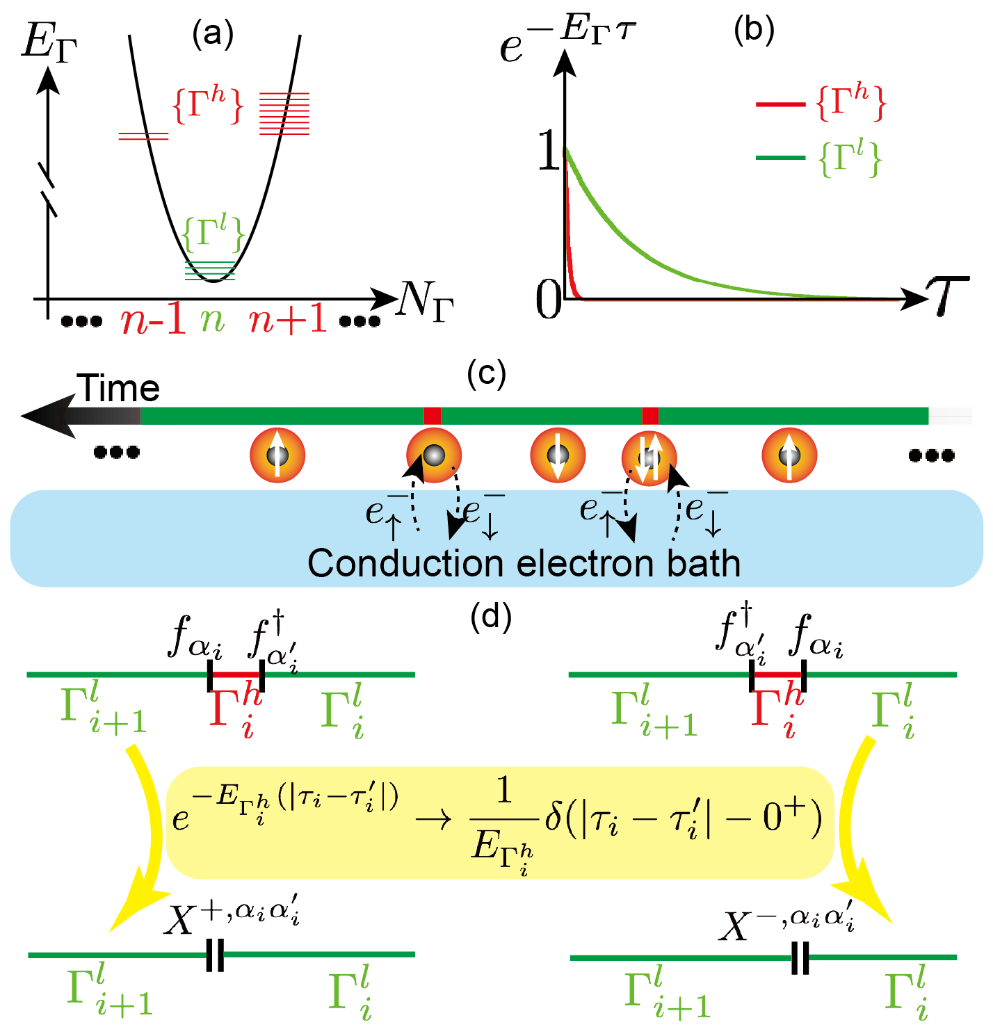
Figure 1: (Color online). Approximations made to CT-HYB in Kondo regime. (a) Energy of atomic multiplets $\Gamma$ as a function of occupation number, in Kondo regime there is $E_{\Gamma}^{h}\gg E_{\Gamma}^{l}$. (b) Schematic plot of $e^{-\Gamma\tau}$ as a function of $\tau$. $e^{-\Gamma^{h}\tau}$ decays much faster than $e^{-\Gamma^{l}\tau}$. (c) Schematic plot of the impurity site hybridizing with the heat bath. In the simplest case of the single orbital model, impurity site spend most of the time on two low energy single occupied states, $|\uparrow\rangle$ and $|\downarrow\rangle$, than on two high energy states, unoccupied $|\rangle$ and double occupied $|\uparrow\downarrow\rangle$ (adapted from Ref. [Kotliar and Vollhardt, 2004]). (d) Sharply decaying imaginary time evolution operator of high energy states is approximated by a normalized Delta function, leading to virtual processes included in $X$ matrix. Left panel, $\tau_{i}>\tau_{i}^{\prime}$; right panel, $\tau_{i}<\tau_{i}^{\prime}$.

The above truncation requires that evolution paths with non-zero contributions to $w_{\text{loc}}(\mathcal{C}_{k})$ are those alternating $\{\Gamma^{h}\}$ and $\{\Gamma^{l}\}$ since

$$|\{\Gamma^{h}|N_{\Gamma^{h}}=n+1\}\rangle \leftarrow f_{\alpha}^{\dagger}|\{\Gamma^{l}|N_{\Gamma^{l}}=n\}\rangle,$$ (13)

$$|\{\Gamma^{h}|N_{\Gamma^{h}}=n-1\} \leftarrow f_{\alpha}|\{\Gamma^{l}|N_{\Gamma^{l}}=n\}\rangle,$$

$$|\emptyset\rangle \leftarrow f_{\alpha}^{\dagger}|\{\Gamma^{h}|N_{\Gamma^{h}}=n+1\}\rangle,$$

$$|\emptyset\rangle \leftarrow f_{\alpha}|\{\Gamma^{h}|N_{\Gamma^{h}}=n-1\}\rangle.$$

$w_{\text{loc}}(\mathcal{C}_{k})$ can be split into two parts according to the energy hierarchy of the head/tail state $\{\Gamma_{1}\}$. The part which starts from and ends in $\{\Gamma_{1}^{h}\}$ is generally much smaller, since it contains more time evolution of the high energy states and thus can be reasonably neglected, especially at very low temperature. Thus, we obtain

$$w_{\text{loc}}(\mathcal{C}_{k}) \approx s_{T_{\tau}}\sum_{\Gamma_{1}^{l}\Gamma_{1}^{h}\cdots\Gamma_{k}^{l}\Gamma_{k}^{h}}e^{-(\beta-\tau_{k})E_{\Gamma_{1}^{l}}}\langle\Gamma_{1}^{l}|f_{\alpha_{k}}|\Gamma_{k}^{h}\rangle$$ (14)

$$\times e^{-(\tau_{k}-\tau_{k}^{\prime})E_{\Gamma_{k}}^{h}}\langle\Gamma_{k}^{h}|f_{\alpha_{k}^{\prime}}^{\dagger}|\Gamma_{k}^{l}\rangle\cdots\langle\Gamma_{2}^{l}|f_{\alpha_{1}^{\prime}}^{\dagger}|\Gamma_{1}^{h}\rangle$$

$$\times e^{-(\tau_{1}^{\prime}-\tau_{1})E_{\Gamma_{1}^{h}}}\langle\Gamma_{1}^{h}|f_{\alpha_{1}}|\Gamma_{1}^{l}\rangle e^{-(\tau_{1}-0)E_{\Gamma_{1}^{l}}},$$

which evolves in $\{\Gamma^{l}\}\leftarrow\{\Gamma^{h}\}\cdots\{\Gamma^{l}\}\leftarrow\{\Gamma^{h}\}\leftarrow\{\Gamma^{l}\}$.

II.3 Energy shift

Eigenvalues of $H_{\text{loc}}$, $\{E_{\Gamma}\}$, can be negative or positive, therefore $e^{-\tau E_{\Gamma}}$($\tau>0$) is either monotonically increasing or decreasing function, respectively. However, it is the relative difference between $\{E_{\Gamma^{h}}\}$ and $\{E_{\Gamma_{l}}\}$ that matters in Monte Carlo simulations. Then it is convenient to make a shift to $\{E_{\Gamma}\}$ such that the time evolution functions appearing in our simulations are always monotonically decreasing. To realize that, we shift the zero of the energy to $E_{0}$, where $E_{0}=\min\{E_{\Gamma^{l}}\}$,

$$E_{\Gamma}\rightarrow E_{\Gamma}^{\prime}=E_{\Gamma}-E_{0}\geq 0.$$ (15)

The transformation is equivalent to multiply a positive factor $e^{\beta E_{0}}$ to $w_{\text{loc}}(\mathcal{C}_{k})$

$$\omega_{\text{loc}}(\mathcal{C}_{k})\rightarrow\omega_{\text{loc}}^{\prime}(\mathcal{C}_{k})=\omega_{\text{loc}}(\mathcal{C}_{k})\times e^{\beta E_{0}},$$ (16)

and partition function is changed to

$$Z\rightarrow Z^{\prime}=Z\times e^{\beta E_{0}}.$$ (17)

Please note that the expectation value of an operator will not be modified by the above transformation,

$$\langle\hat{O}\rangle_{Z^{\prime}} =\frac{\int d\mathcal{C}w^{\prime}(\mathcal{C})O(\mathcal{C})}{Z^{\prime}}=\frac{\int d\mathcal{C}w(\mathcal{C})e^{\beta E_{0}}O(\mathcal{C})}{Z\times e^{\beta E_{0}}}$$ (18)

$$=\frac{\int d\mathcal{C}w(\mathcal{C})O(\mathcal{C})}{Z}=\langle\hat{O}\rangle_{Z}.$$

Prime $\prime$ is omitted for $E_{\Gamma}^{\prime}$, $Z^{\prime}$, etc. hereafter for the sake of simplicity.

II.4 Approximations in Kondo limit

Two typical fragments of evolution paths appearing in $w_{\text{loc}}(\mathcal{C}_{k}$) in Eq. (14) are schematically depicted in Fig. 1(d) where each high energy state is sandwiched between one creation and one annihilation operators. Here we focus on the left panel where $\tau_{i}>\tau_{i}^{\prime}$. In the limit of $E_{\Gamma_{i}^{h}}\rightarrow+\infty$, the probability of finding a configuration with finite $\tau=\tau_{i}-\tau_{i}^{\prime}>0$ approaches 0 due to the exponentially decreasing factor $e^{-(\tau_{i}-\tau_{i}^{\prime})E_{\Gamma_{i}^{h}}}$, which means that excitations to high energy states are instantaneous, i.e. $\tau_{i}-\tau_{i}^{\prime}=0^{+}$, in the Kondo limit. Integrating over $\tau_{i}^{\prime}$, we obtain

$$\int_{\tau_{i-1}}^{\tau_{i}}e^{-(\tau_{i}-\tau_{i}^{\prime})E_{\Gamma_{i}^{h}}}d\tau_{i}^{\prime}\cdots=\cdots\frac{1}{E_{\Gamma_{i}^{h}}}\cdots|_{E_{\Gamma_{i}^{h}}\rightarrow+\infty},$$ (19)

where $\frac{1}{E_{\Gamma_{i}^{h}}}$ indicates total probability for this particular type of virtual processes. Then in the Kondo limit, where all the high energy local atomic states can be treated as the virtual processes, the sharply decreasing time evolution can be well approximated by a probability normalized delta function

$$e^{-(\tau_{i}-\tau_{i}^{\prime})E_{\Gamma_{i}^{h}}}\rightarrow\frac{1}{E_{\Gamma_{i}^{h}}}\delta(\tau_{i}-\tau_{i}^{\prime}-0^{+}).$$ (20)

This approximation is getting better and better when the charging energy $E_{\Gamma^{h}}$ is approaching infinity, which is very suitable for the heavy fermion systems at the Kondo limit. The above approximation has the following advantages. 1) By neglecting the time dependence of the local propagator for the high energy atomic states, the charge fluctuations to these high energy atomic states will be treated as the virtual processes, which induce an effective exchange coupling among the conduction electrons and the low energy atomic states. For simple model system, i.e. the single orbital Anderson impurity model, it can automatically obtain the exact same coupling terms as the SWT. 2) This approximation can be easily applied to more realistic models generated during the process of LDA+DMFT, the coupling terms between the f-electrons and conduction electrons have the momentum and orbital dependence, which make SWT very difficult.

Replacing all $e^{-\tau\cdot E_{\Gamma^{h}}}$ with $\frac{1}{E_{\Gamma^{h}}}\delta(\tau-0^{+})$ and integrating over all $\{\tau_{i}^{\prime}\}$, we find that a creation operator and an annihilation operator always appear in adjacent pairs. The configuration space now reads

$$\mathcal{C} =\{\{\},\{\tau_{1};s_{1}f_{\alpha_{1}}f_{\alpha_{1}}^{\dagger}\},\cdots,$$ (21)

$$\times\{\tau_{1},\cdots,\tau_{k};\>s_{1}f_{\alpha_{1}}f_{\alpha_{1}^{\prime}}^{\dagger},\cdots,s_{k}f_{\alpha_{k}}f_{\alpha_{k}^{\prime}}^{\dagger}\},\cdots\},$$

where

$$s_{i}f_{\alpha_{i}}f_{\alpha_{i}^{\prime}}^{\dagger}|_{s_{i}=1} \equiv f_{\alpha_{i}}f_{\alpha_{i}^{\prime}}^{\dagger}\rightarrow\tau_{i}=\tau_{i}^{\prime}+0^{+},$$ (22)

$$s_{i}f_{\alpha_{i}}f_{\alpha_{i}^{\prime}}^{\dagger}|_{s_{i}=-1} \equiv f_{\alpha_{i}^{\prime}}^{\dagger}f_{\alpha_{i}}\rightarrow\tau_{i}=\tau_{i}^{\prime}-0^{+}.$$

Summation over $\{\Gamma^{h}\}$ can be written in a compact form by defining two types of $X$-matrices labelled by $s$

$$X_{\Gamma_{i+1}^{l}\Gamma_{i}^{l}}^{s_{i}\alpha_{i}\alpha_{i}^{\prime}}|_{s_{i}=1} \equiv\sum_{\Gamma_{i}^{h}}\langle\Gamma_{i+1}^{l}|f_{\alpha_{i}}|\Gamma_{i}^{h}\rangle\frac{1}{E_{\Gamma_{i}^{h}}}\langle\Gamma_{i}^{h}|f_{\alpha_{i}^{\prime}}^{\dagger}|\Gamma_{i}^{l}\rangle,$$ (23)

which describes virtual charge excitations $f^{n}\rightarrow f^{n+1}$ and

$$X_{\Gamma_{i+1}^{l}\Gamma_{i}^{l}}^{s_{i}\alpha_{i}\alpha_{i}^{\prime}}|_{s_{i}=-1} \equiv\sum_{\Gamma_{i}^{h}}\langle\Gamma_{i+1}^{l}|f_{\alpha_{i}^{\prime}}^{\dagger}|\Gamma_{i}^{h}\rangle\frac{1}{E_{\Gamma_{i}^{h}}}\langle\Gamma_{i}^{h}|f_{\alpha_{i}}|\Gamma_{i}^{l}\rangle,$$ (24)

which describes virtual charge excitations from $f^{n}\rightarrow f^{n-1}$ . Finally one obtains the partition function

$$Z \approx Z_{\text{bath}}\sum_{k=0}^{\infty}\int_{0}^{\beta}d\tau_{1}\cdots\int_{\tau_{k-1}}^{\beta}d\tau_{k}\sum_{\begin{subarray}{c}\alpha_{1}\cdots\alpha_{k}\\ \alpha_{1}^{\prime}\cdots\alpha_{k}^{\prime}\end{subarray}}s_{T_{\tau}}$$ (25)

$$\times w_{\text{loc}}(\mathcal{C}_{k})\prod_{\alpha}\det(\mathcal{M}_{\alpha}^{(k_{\alpha})})^{-1},$$

where the local trace is reformulated in terms of $X$-matrices as

$$w_{\text{loc}}(\mathcal{C}_{k}) =\sum_{\Gamma_{1}^{l}\cdots\Gamma_{k}^{l}}e^{-(\beta-\tau_{k})E_{\Gamma_{1}^{l}}}X_{\Gamma_{1}^{l}\Gamma_{k}^{l}}^{s_{k}\alpha_{k}\alpha_{k}^{\prime}}e^{-(\tau_{k}-\tau_{k-1})E_{\Gamma_{k}^{l}}}$$ (26)

$$\times\cdots X_{\Gamma_{3}^{l}\Gamma_{2}^{l}}^{s_{2}\alpha_{2}\alpha_{2}^{\prime}}e^{-(\tau_{2}-\tau_{1})E_{\Gamma_{2}^{l}}}X_{\Gamma_{2}^{l}\Gamma_{1}^{l}}^{s_{1}\alpha_{1}\alpha_{1}^{\prime}}e^{-(\tau_{1}-0)E_{\Gamma_{1}^{l}}}.$$

An example of third order configuration $\mathcal{C}_{3}$ is schematically shown in Fig. 2(a) and its determinant part is

$$w_{\det}(\mathcal{C}_{3})=\left|\begin{array}[]{ccc}\triangle_{\alpha_{1}^{\prime}\alpha_{1}}(0^{-})&\triangle_{\alpha_{1}^{\prime}\alpha_{2}}(\tau_{1}-\tau_{2})&\triangle_{\alpha_{1}^{\prime}\alpha_{3}}(\tau_{1}-\tau_{3})\\ \triangle_{\alpha_{2}^{\prime}\alpha_{1}}(\tau_{2}-\tau_{1})&\triangle_{\alpha_{2}^{\prime}\alpha_{2}}(0^{+})&\triangle_{\alpha_{2}^{\prime}\alpha_{3}}(\tau_{2}-\tau_{3})\\ \triangle_{\alpha_{3}^{\prime}\alpha_{1}}(\tau_{3}-\tau_{1})&\triangle_{\alpha_{3}^{\prime}\alpha_{2}}(\tau_{3}-\tau_{2})&\triangle_{\alpha_{3}^{\prime}\alpha_{3}}(0^{-})\end{array}\right|,$$ (27)

which can be expanded into $3!=6$ terms as schematically represented in Fig. 2(b-g).

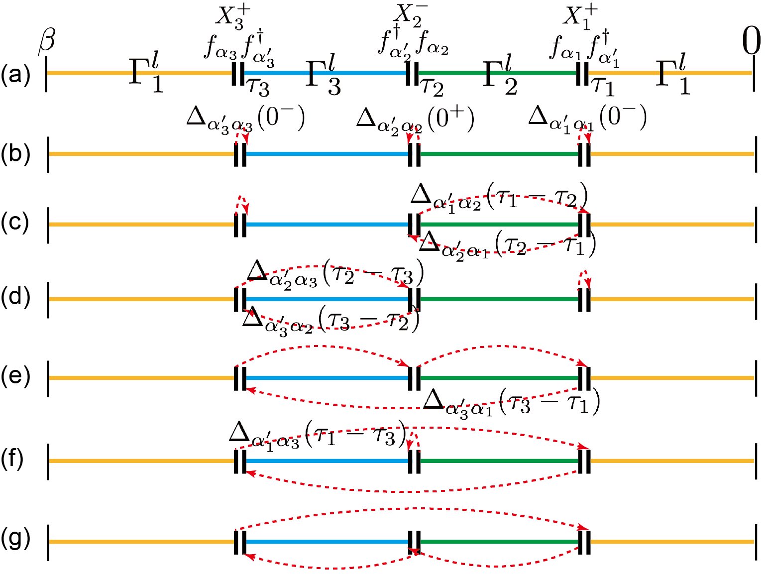
Figure 2: (Color online) Schematic plot of a third order configuration in the approximated partition function Eq. (25). (a), The evolution of low energy states ($\Gamma^{l}_{i}$, labelled by horizontal solid colored lines) by means of virtual processes. Two adjacent vertical solid black lines are to denote the creation and annihilation operator pair in an $X$ matrix. $\pm$ in $X^{\pm}_{i}$ is to denote the type ($s_{i}=\pm 1$) of $X$ matrices defined in Eq. (23, 24). (b-g), Illustration of the hybridizations determinant, Eq. (27), by arrowed dashed red lines starting from a annihilation operator and ending at a creation operator. For a three order term, there are $3!=6$ terms in the determinant.

III Monte Carlo sampling

Before introducing the detail of the Monte Carlo sampling, we first divide the different pair operators into the following types

• pure-pair: $\alpha_{i}=\alpha_{i}^{\prime}$, $sf_{\alpha_{i}}f_{\alpha_{i}}^{\dagger}$,

• mix-pair: $\alpha_{i}\neq\alpha_{i}^{\prime}$, $s_{i}f_{\alpha_{i}}f_{\alpha_{i}^{\prime}}^{\dagger}$.

An $k$-th order configuration $\mathcal{C}_{k}$ consists of time-ordered pure-pairs and mix-pairs

$$\beta\vdash s_{k}f_{\alpha_{k}}f_{\alpha_{k}^{\prime}}^{\dagger}(\tau_{k})-\cdots-s_{1}f_{\alpha_{1}}f_{\alpha_{1}^{\prime}}^{\dagger}(\tau_{1})\dashv 0.$$ (28)

$\mathcal{C}_{k}$ contains an equal number of creation and annihilation operators for each flavor by construction. With fixed $\{\tau_{i}\}$ and fixed number of single-particle operators of each flavor, $\mathcal{C}_{k}$ is mathematically an element in the set of direct products of operators permutations $\mathscr{P}$,

$$\{\mathcal{C}_{ki}\} =\{\mathscr{P}\{f_{\alpha_{k}},\cdots,f_{\alpha_{1}}\}\bigotimes\mathscr{P}\{f_{\alpha_{k}^{\prime}}^{\dagger},\cdots,f_{\alpha_{1}^{\prime}}^{\dagger}\}$$ (29)

$$\bigotimes\prod_{i=1}^{k}\mathscr{P}\{f_{\alpha_{i}},f_{\alpha_{i}^{\prime}}^{\dagger}\}\}.$$

Based on the fact that any permutation can be expressed as the product of transpositions, we design updates which keep diagram order as the following,

• left-exchange: exchange annihilation operators of two adjacent pairs,

• right-exchange: exchange creation operators of two adjacent pairs,

• in-pair swap: $s_{i}\rightarrow-s_{i}$.

Ergodicity can be satisfied by the above updates together with insertion and removal of pure-pairs at random times which change expansion order by 1, since any $\mathcal{C}_{ki}$ can be generated from an list of pure pairs by successive transpositions. Updates which shift pair-operators is not necessary but is useful to increase sampling efficiency.

Metropolis-Hastings algorithm is used to sample configuration space $\mathcal{C}$ according to the configuration weight $w(\mathcal{C}_{k})=w_{\text{loc}}(\mathcal{C}_{k})\prod_{\alpha}\det(\mathcal{M}_{\alpha}^{(\mathcal{C}_{k})})^{-1}d\tau^{k}$. The random walk in $\mathcal{C}$ must satisfy detailed balance condition and ergodicity.

In the following, we first discuss the update scheme for general interaction and then for density-density iteration. The main difference between the two is the way to calculate local trace.

III.1 General interactions

As shown in Eq. (26), the calculation of local trace requires multiplication of matrices and is time-consuming. We can take advantages of symmetries of $H_{\text{loc}}$ and divide the full Hilbert space of $H_{\text{loc}}$ into much smaller subspaces labeled by some good quantum numbers (GQNs)Haule [2007], such as the total particle number $N_{\text{tot}}$, the total Spin $z$-component $S_{\text{tot}}^{z}$, the total angular momentum $J_{z}$, etc. Single particle creation and annihilation operators are therefore in block diagonal form, which speeds up the calculation. Further speed-up can be achieved by using the divide-and-conquerHuang et al. [2015] trick based on the fact that diagrammatic configurations are modified locally in each update.

III.1.1 Pure-pair insertion/removal

To insert a pure-pair in configuration $\mathcal{C}_{k}$, we pick a random flavor $\alpha$, a random pair with type $s$, and a random time $\tau$ in $(0,\beta)$. In the corresponding removal process, we simply delete one of the existing pure-pairs among $k_{\alpha}+1$ pairs. The ratio of the transition probabilities can be calculated for the inserting case as

$$\frac{p(k_{\alpha}\rightarrow k_{\alpha}+1)}{p(k_{\alpha}+1\rightarrow k_{\alpha})}=\frac{w_{\text{loc}}(\mathcal{C}_{k+1})\det(\mathcal{M}_{\alpha}^{(\mathcal{C}_{k+1})})^{-1}}{w_{\text{loc}}(\mathcal{C}_{k})\det(\mathcal{M}_{\alpha}^{(\mathcal{C}_{k})})^{-1}}\times\frac{2\beta}{k_{\alpha}+1},$$ (30)

where $w_{\text{loc}}(\mathcal{C}_{k+1})$ is the local trace and $(\mathcal{M}_{\alpha}^{(\mathcal{C}_{k+1})})^{-1}$ is the hybridization matrix of the new configuration at order $k+1$.

III.1.2 Left/right-exchange

In the left-exchange update, we randomly pick a pair operator $s_{i}f_{\alpha_{i}}f_{\alpha_{i}^{\prime}}^{\dagger}$ together with its left neighbor $s_{i+1}f_{\alpha_{i+1}}f_{\alpha_{i+1}^{\prime}}^{\dagger}$ and exchange their annihilation operators if $\alpha_{i}\neq\alpha_{i+1}$

$$\cdots-s_{i+1}f_{\alpha_{i+1}}f_{\alpha_{i+1}^{\prime}}^{\dagger}(\tau_{i+1}) -s_{i}f_{\alpha_{i}}f_{\alpha_{i}^{\prime}}^{\dagger}(\tau_{i})-\cdots$$ (31)

$$\Downarrow$$

$$\cdots-s_{i+1}f_{\alpha_{i}}f_{\alpha_{i+1}^{\prime}}^{\dagger}(\tau_{i+1}) s_{i}f_{\alpha_{i+1}}f_{\alpha_{i}^{\prime}}^{\dagger}(\tau_{i})-\cdots.$$

If $i=k$, the right-most pair is selected as the left neighbor of $k$-th pair$(k\geq 2)$. It is equivalent to two successive shifts: $f_{\alpha}$ from $\tau_{i+1}$ to $\tau_{i}$ and $f_{\alpha_{i+1}}$ from $\tau_{i}$ to $\tau_{i+1}$. Using Metropolis-Hasting algorithm we obtain

$$\frac{p(k)^{\prime}}{p(k)}=\frac{w_{\text{loc}}(\mathcal{C}_{k}^{\prime})}{w_{\text{loc}}(\mathcal{C}_{k})}\times\frac{\det(\mathcal{M}_{\alpha_{i}}^{(\mathcal{C}^{\prime}_{k})})^{-1}}{\det(\mathcal{M}_{\alpha_{i}}^{(\mathcal{C}_{k})})^{-1}}\times\frac{\det(\mathcal{M}_{\alpha_{i+1}}^{(\mathcal{C}^{\prime}_{k})})^{-1}}{\det(\mathcal{M}_{\alpha_{i+1}}^{(\mathcal{C}_{k})})^{-1}},$$ (32)

where $(\mathcal{M}_{\alpha}^{(\mathcal{C}^{\prime}_{k})})^{-1}$ ($\alpha=\alpha_{i},\alpha_{i+1}$) is the new hybridization matrix of flavor $\alpha$ with shifted $f_{\alpha}$ compared with original $(\mathcal{M}_{\alpha}^{(\mathcal{C}_{k})})^{-1}$.

The right-exchange updates works quite similar to left-exchange except that it operates on creation operators, and the detailed balance condition is of the form of Eq. (32) where $(\mathcal{M}_{\alpha}^{(\mathcal{C}^{\prime}_{k})})^{-1}$ is hybridization matrix with $f_{\alpha}^{\dagger}$ being shifted.

III.1.3 Swap

The $i$th pair is randomly selected, and we flip its type from $s_{i}$ to $-s_{i}$. Swap update is very important for satisfying ergodicity since it switches virtual charge fluctuations between $f^{n}\rightarrow f^{n-1}$ and $f^{n}\rightarrow f^{n+1}$. Pure-pair will not be selected since the swap of pure-pair can be done by removal of $s_{i}f_{\alpha_{i}}f_{\alpha_{i}^{\prime}}^{\dagger}$ and insertion of $-s_{i}f_{\alpha_{i}}f_{\alpha_{i}^{\prime}}^{\dagger}$ at $\tau_{i}$ successively. The ratio of the transition probabilities is

$$\frac{p(k)^{\prime}}{p(k)}=\frac{w_{\text{loc}}(\mathcal{C}_{k}^{\prime})}{w_{\text{loc}}(\mathcal{C}_{k})},$$ (33)

The reason why $\mathcal{M}^{-1}$ is not involved in Eq. (33) is that it’s block diagonal in spin-orbitals.

III.2 Density-Density interactions

If $H_{loc}$ commutes with the occupation number operator of each orbital, the eigenstates of $H_{loc}$ are Fock states. For each orbital, creation operator has to be followed by an annihilation operator for all valid configurations(we refer it as NN-Rule). The weighting factor of the allowed configuration $\mathcal{C}_{k}$ can then be expressed as

$$w_{\text{loc}}(\mathcal{C}_{k}) =s_{T_{\tau}}\cdot e^{-(\beta-\tau_{k})E_{\Gamma_{1}^{l}}}X_{\Gamma_{1}^{l}\Gamma_{k}^{l}}^{s_{k}\alpha_{k}\alpha_{k}^{\prime}}e^{-(\tau_{k}-\tau_{k-1})E_{\Gamma_{k}^{l}}}\cdots$$ (34)

$$\times X_{\Gamma_{3}^{l}\Gamma_{2}^{l}}^{s_{2}\alpha_{2}\alpha_{2}^{\prime}}e^{-(\tau_{2}-\tau_{1})E_{\Gamma_{2}^{l}}}X_{\Gamma_{2}^{l}\Gamma_{1}^{l}}^{s_{1}\alpha_{1}\alpha_{1}^{\prime}}e^{-(\tau_{1}-0)E_{\Gamma_{1}^{l}}}.$$

To propose valid configurations, updates should be carefully designed to satisfy the NN-Rule.

III.2.1 Pure-pair insertion/removal

The main difference with the general interaction case is that the pair type $s$ can not be randomly selected. For a given configuration, if the orbital $\alpha$ is occupied (unoccupied) in the Fock state spanning $\tau$, only the insertion of $f_{\alpha}^{\dagger}f_{\alpha}$($f_{\alpha}f_{\alpha}^{\dagger}$) at $\tau$ is allowed. When it comes to pure-pair removal, we correspondingly delete $f_{\alpha}^{\dagger}f_{\alpha}$ ($f_{\alpha}^{\dagger}f_{\alpha}$) away from $\tau$. The condition for detail balance reads

$$\frac{p(k_{\alpha}\rightarrow k_{\alpha}+1)}{p(k_{\alpha}+1\rightarrow k_{\alpha})}=\frac{w_{\text{loc}}(\mathcal{C}_{k+1})\det(\mathcal{M}_{\alpha}^{(\mathcal{C}_{k+1})})^{-1}}{w_{\text{loc}}(\mathcal{C}_{k})\det(\mathcal{M}_{\alpha}^{(\mathcal{C}_{k})})^{-1}}\times\frac{\beta}{k_{\alpha}+1}.$$ (35)

III.2.2 Left/right-exchange and swap

Exchange process which violate the NN-Rule will be directly rejected. Swap updates will not violate the rule since only mix-pairs are swapped. The conditions for the detailed balance are same with those of general interactions except for the calculations of local trace. While left/right-exchange is equivalent to shift of segments, swap is equivalent to switch between infinitesimal small segment and anti-segment.

IV Measurements

The most important observable for QMC impurity solvers is the finite temperature imaginary-time Green’s function defined by $G_{\alpha\alpha^{\prime}}^{f}(\tau)=-\langle\mathcal{T}_{\tau}f_{\alpha}(\tau)f_{\alpha^{\prime}}^{\dagger}(0)\rangle$. The single particle green’s function, in general, includes high energy process that involve states with different occupation numbers. Such process, however, are missing in our approximated parition function, Eq. (25), in the Kondo limit, where charge fluctuations are projected out completely. Nevertheless, we can still measure the low-energy contributions to $G_{\alpha\alpha^{\prime}}^{f}(\tau)$, which correspond to the quasi-particle part in the single-particle excitations. Here, we give a brief descriptions of how to measure $G_{\alpha\alpha^{\prime}}^{f}(\tau)$. The step by step derivation of the measurement formula is given in Appendix B.

In the CTQMC, the diagrams contributing to $G_{\alpha\alpha^{\prime}}^{f}(\tau)$ can be generated from diagrams in $Z$: One chooses an arbitrary pair of creation and annihilation operators in a given configuration $\mathcal{C}_{k}$, and removes the corresponding contributions to the determinant $\Delta_{\alpha}^{(\mathcal{C}_{k})}$. Within the approximation applied to the partition function, only a specific pairs of creation and annihilation operators have contributions to $G_{\alpha\alpha^{\prime}}^{f}(\tau)$. A pair of operators that belong to different $X$ matrices does contribute, while those on the same $X$ matrix do not. Those diagrams are illustrated in Fig. 3(b) and Fig. 3(c), respectively.

The measurement formula is thus given by

$$G^{f}_{\alpha\alpha^{\prime}}(\tau)=-\langle\frac{1}{\beta}\sideset{}{{}^{\prime}}{\sum}_{m,n=1}^{k}\delta_{\alpha_{m},\alpha}\delta_{\alpha_{n}^{\prime},\alpha^{\prime}}\delta^{-}[\tau-(\tau_{m}-\tau_{n})]\mathcal{M}_{nm}^{(\mathcal{C}_{k})}\rangle_{Z},$$ (36)

where $\prime$ stands for the resctriction of summations to $m\neq n$ ( $m$ and $n$ are one different $X$ matrices). The function $\delta^{-}$ is defined by $\delta^{-}(\tau-\tau^{\prime})=\delta(\tau-\tau^{\prime})$ for $\tau>0$, and $\delta^{-}(\tau-\tau^{\prime})=-\delta(\tau-\tau^{\prime}-\beta)$ for $\tau<0$. After the Fourier transform, we obtain

$$G_{\alpha\alpha^{\prime}}^{f}(i\omega_{l})=-\langle\frac{1}{\beta}\sideset{}{{}^{\prime}}{\sum}_{m,n=1}^{k}\delta_{\alpha_{m},\alpha}\delta_{\alpha_{n}^{\prime},\alpha^{\prime}}\mathcal{M}_{nm}^{(\mathcal{C}_{k})}e^{i\omega_{l}(\tau_{m}-\tau_{n})}\rangle.$$ (37)

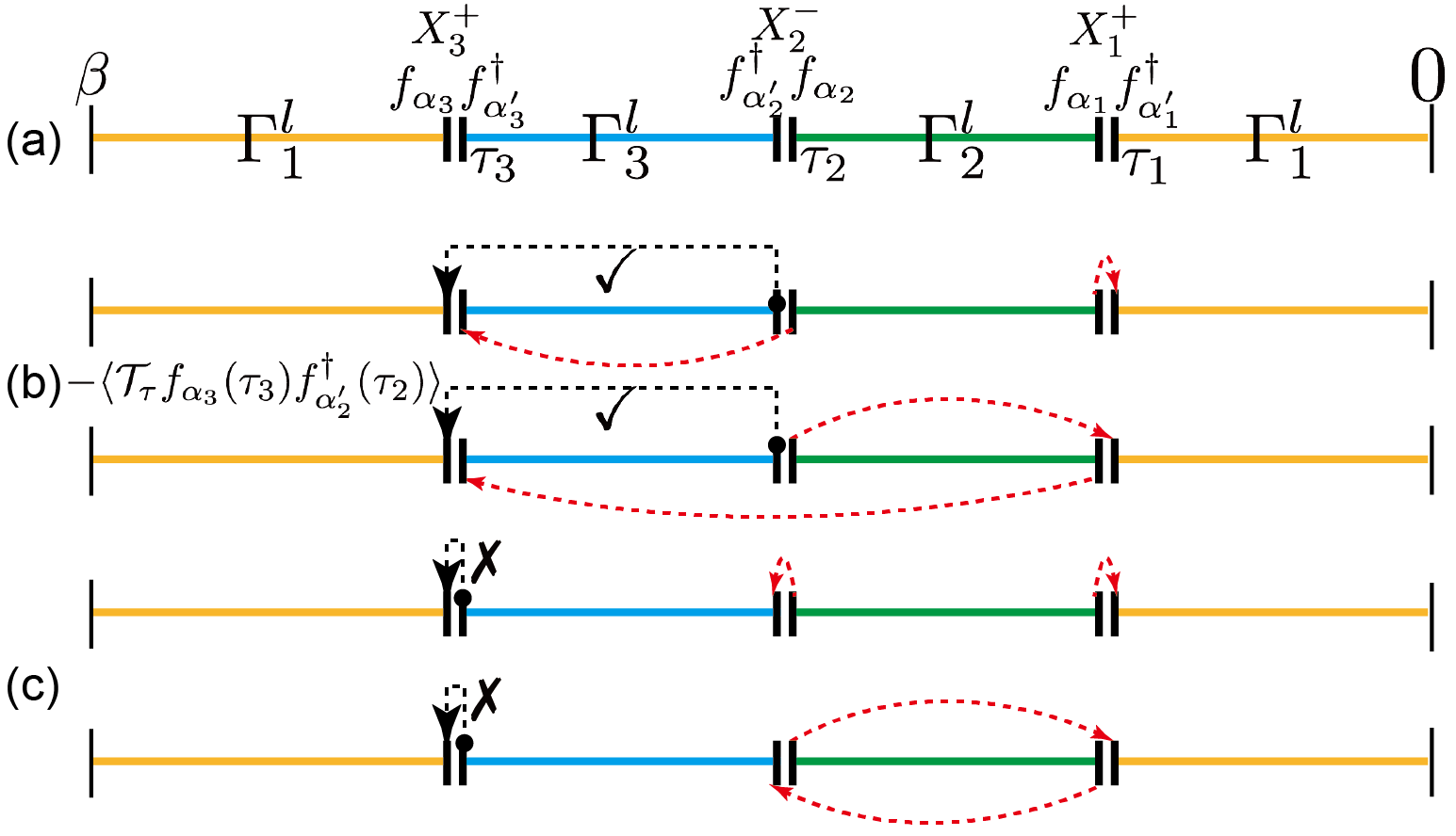
Figure 3: (Color online) Schematic plot of a third order configuration for measurement of Green’s function in Kondo regime. (a) Local trace part of Green’s function $G_{\alpha\alpha}^{f}(\tau)$, which is the same as that of $Z$ shown in Fig. 2(a). (b) An example of allowed (marked by ✓) measurement for $G_{\alpha\alpha}^{f}(\tau)$. Two operators from two different $X$ matrices [here $f_{\alpha_{3}}(\tau_{3})$ of pair $X_{3}$ and $f_{\alpha^{\prime}_{2}}^{\dagger}(\tau_{2})$ of pair $X_{2}$] are identified as operators in $G_{\alpha\alpha}^{f}(\tau)$. In upper and lower panels, we plot existing hybridization lines which do not connect between the selected operators. (c) An example of forbidden (marked by ✗) measurement in $G_{\alpha\alpha}^{f}(\tau)$. Two operators belonging to the same $X$ matrix are not allowed to be chosen in measurement.

We can compare the present measurement formula, Eq. (36), with that for the of $t$-matrix in the CS model, Eq. (9) in Ref. [Otsuki et al., 2007]. They are related by $t(\tau)=V^{2}G(\tau)$ if there is no $k$ dependence in $V_{k}$.

The asymptotic behavior of $G(i\omega_{n})$ is $i\omega_{n}*G(i\omega_{n})|_{n\rightarrow\infty}=z$ with $z<1$ being the quasi-particle weight in the Kondo limit.

The measurement formula for the two particle correlation function bear exactly the same form as Eq. (11)-(13) of Ref. [Otsuki et al., 2007], which are not mentioned here.

V Benchmarks

While Coqblin-Shrieffer(CS) model is a low energy effective Hamiltonian of ASIM in large $U$ limit in which only virtual excitations $f^{1}\rightarrow f^{0}$ survive, Kondo model incorporates both $f^{1}\rightarrow f^{0}$ and $f^{1}\rightarrow f^{2}$ by assuming deep impurity level $\epsilon_{f}$ and large $U$. Both the two models can be derived by SWT from SIAM with density-density interaction shown below

$$H =\sum_{k\alpha}\epsilon_{k}c_{k\alpha}^{\dagger}c_{k\alpha}+\sum_{\alpha=-j}^{j}\varepsilon_{\alpha}n_{\alpha}+U\sum_{\alpha<\alpha^{\prime}}n_{\alpha}n_{\alpha^{\prime}},$$ (38)

$$+\sum_{\alpha k}[V_{k}^{\alpha}f_{\alpha}^{\dagger}c_{k\alpha}+V_{k}^{\alpha*}c_{k\alpha}^{\dagger}f_{\alpha}],$$

with $N=2j+1$. A constant density of states $\rho(\epsilon)=\frac{1}{2D}\theta(D-|\epsilon|)$ with $D=1$ is chosen for conduction electrons. Both the CS and Kondo models are derived from SIAM under certain conditions. Therefore the comparison between the Monte Carlo simulations on these models using CT-J method and directly on SIAM using our new method proposed in this paper can be used as the benchmark. For sake of simplicity, our CT-QMC formalism for partition function (25) is referred as CT-X, where “X” refers to $X$-matrices.

V.1 CS model

The CS model reads

$$H_{0} =\sum_{k\alpha}\epsilon_{k}c_{k\alpha}^{\dagger}c_{k\alpha}+\sum_{\alpha}(\varepsilon_{\alpha}+J_{\alpha\alpha})|\alpha\rangle\langle\alpha|,$$ (39)

$$H_{1} =\sum_{\alpha\alpha^{\prime}}J_{\alpha\alpha^{\prime}}|\alpha\rangle\langle\alpha^{\prime}|(-c_{\alpha}c_{\alpha^{\prime}}^{\dagger}),$$ (40)

where $c_{\alpha}=N_{0}^{-1/2}\sum_{k}c_{k\alpha}$, with $N_{0}$ being number of sites and $\alpha$ denotes the spin/orbital indices. Partition function of CS model in CT-J can be obtained by applying the following restrictions to Eq. (24) and Eqs. (25)–(26):

• $V_{k}^{\alpha}=V_{k}^{\alpha*}=V^{\alpha}$, since exchange parameters in CS model can be chosen as momentum independent;

• $J_{\alpha\alpha^{\prime}}\equiv\frac{V_{\alpha}V_{\alpha^{\prime}}}{-\min\{\varepsilon_{\alpha}\}}$, where $E_{\Gamma^{h}}=-\min\{\varepsilon_{\alpha}\}$ is the shifted energy of $f^{0}$ state;

• $X^{-1,\alpha\alpha^{\prime}}$ has only one none-zero element $X_{|\alpha\rangle|\alpha^{\prime}\rangle}^{-1,\alpha\alpha^{\prime}}=\frac{1}{-\min\{\varepsilon_{\alpha}\}}|\alpha\rangle\langle\alpha^{\prime}|$.

To simulate the CS model, we should put an additional restriction to $\mathcal{C}_{k}$ with $\{s_{i}=-1|i=1,\cdots,k\}$, which means that only pair operators describing $f^{1}\rightarrow f^{0}$ enters in $\mathcal{C}_{k}$. Furthermore, intra-pair swap update is forbidden since it gives rise to virtual excitation $f^{1}\rightarrow f^{2}$ which is absent in the CS model.

V.1.1 t-matrix

To test CT-X, we calculate t-matrix with $N=8$ and compare it with the results obtained by CT-J. We choose the exchange parameter $J=\frac{V^{2}}{-\epsilon_{f}}$ to be 0.075 and temperature $T=0.001D$. The results obtained by CT-X and CT-J are plotted together in FIG. 4, which show excellent agreement.

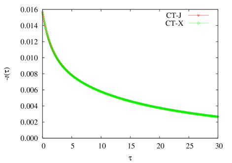
Figure 4: The impurity t-matrix $t_{\alpha}(\tau)$ in the imaginary-time domain for $N=8$, $J=0.075$ and $T=0.001$. Datas of CT-J is obtained from Fig. 7 in Ref. [Otsuki et al., 2007].

V.1.2 static susceptibility

The static susceptibility is evaluated by integrating dynamical susceptibility $\chi(\tau)$ as introduced in detail in section 2.3 of Ref. [Otsuki et al., 2007]. The results obtained by CT-X and CT-J are shown in FIG. 5. Again they match each other very well.

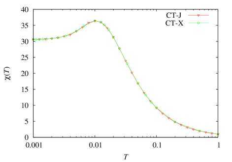
Figure 5: Temperature dependence of the static susceptibility $\chi$ for N=8 and J=0.075. Datas of CT-J is obtained from Fig. 6 in Ref. [Otsuki et al., 2007].

V.2 Kondo model

The Kondo model is given by

$$H=\sum_{k\sigma}\epsilon_{k}c_{k\sigma}^{\dagger}c_{k\sigma}+J\boldsymbol{S}\cdot\boldsymbol{\sigma}_{c}.$$ (41)

where $\boldsymbol{S}=\sum_{\alpha\beta}f_{\alpha}^{\dagger}\boldsymbol{\sigma}_{\alpha\beta}f_{\beta}$ and $\boldsymbol{\sigma}_{c}=\sum_{\sigma\sigma^{\prime}}c_{\sigma}^{\dagger}\boldsymbol{\sigma}_{\sigma\sigma^{\prime}}c_{\sigma^{\prime}}$ denoting the spin operators of the local moments and itinerant electrons respectively. The spin-spin exchange terms can be obtained by considering both of the two virtual processes $f^{1}\rightarrow f^{0}$ and $f^{1}\rightarrow f^{2}$. With the particle-hole symmetry, we set $U=-2\epsilon_{f}$ thus $J=\frac{V^{2}}{-\epsilon_{f}}=\frac{V^{2}}{U+\epsilon_{f}}$ . To simulate the Kondo model by our CT-X method, all types of pair operators are allowed to appear in the MC configurations.

As a benchmark, we calculated the $t$-matrix with $J$=0.3 and $T$=0.001 by CX-T and compare it with the results obtained by CT-J In FIG. 6. Again the results from CT-X and CT-J agree very well indicating that CT-X can treat two types of virtual charge fluctuations well. With the particle-hole symmetry of Kondo model, the real part of $t(i\omega_{n})$ is zero and hence not plotted in FIG. 6.

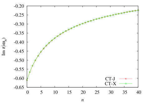
Figure 6: Imaginary part of the impurity t-matrix $t(i\omega_{n})$ of the Kondo model in the imaginary-frequency domain for N=2 and J=0.300. Note: datas of CT-J in this figure is collected by means of WebPlotDigitizer Rohatgi from Fig. 11. in Ref. [Otsuki et al., 2007].

V.3 Kondo lattice model (KLM)

KLM reads

$$H=\sum_{k\sigma}\epsilon_{k}c_{k\alpha}^{\dagger}c_{k\alpha}+J\sum_{i}S_{i}\cdot\boldsymbol{\sigma}_{i}.$$ (42)

To further test this new impurity solver, we perform DMFT calculations on KLM in the infinite-dimension hyper-cubic lattice with the density of states $\rho_{c}(\omega)=D^{-1}\sqrt{2/\pi}exp(-2\omega^{2}/D^{2})$. We set $D=1$ and fix the conduction-electron density per site as $n_{c}=0.9$ as that in Ref. [Otsuki et al., 2009]. The DMFT is iterated on conduction-electron self-energy $\Sigma_{c}$$(i\omega_{n})$, which is related to the cavity Green function $\mathcal{G}_{c}^{0}$ and the measured impurity $t$-matrix by Dyson equation $\Sigma_{c}(i\omega_{n})^{-1}=t(i\omega_{n})+\mathcal{G}_{c}^{0}(i\omega_{n})$. For sake of benchmark, we calculate the momentum distribution of conduction electrons:

$$n_{c}(\boldsymbol{\kappa})=\langle c_{k\sigma}^{\dagger}c_{k\sigma}\rangle=T\sum_{n}G_{c}(\boldsymbol{\kappa},i\omega_{n})e^{i\omega_{n}0^{+}},$$ (43)

where $\boldsymbol{\kappa}\equiv\epsilon_{k}$ and $G_{c}$ is the conduction-electron Green function in the KLM, $G_{c}(\boldsymbol{\kappa},i\omega_{n})=[i\omega_{n}-\boldsymbol{\kappa}+\mu-\Sigma_{c}(i\omega_{n})]^{-1}$. FIG. 7 shows the temperature dependence of $n_{c}(\boldsymbol{\kappa})$ at T=0.0050, 0.0025 and 0.0010 and well reproduces the evolution of Fermi surface as shown in FIG. 4 of Ref. [Otsuki et al., 2009]. For comparison, we plot in FIG. 8 the results computed by CT-X together with results computed by CT-X at T=0.001. Once again it demonstrates that CT-X can treat two types of virtual charge fluctuations well.

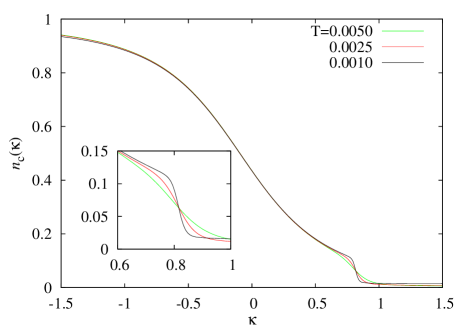
Figure 7: (Color online). Temperature dependence of momentum distribution $n_{c}(\boldsymbol{\kappa})$ computed by CT-X for $J$=0.3 and $n_{c}$=0.9. The vicinity of the large Fermi surface is enlarged in the inset.

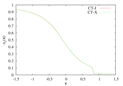
Figure 8: (Color online). Momentum distribution $n_{c}(\boldsymbol{\kappa})$ at T=0.001 and comparison with the CT-X. Datas of CT-J is obtained from Fig. 74 in Ref. [Otsuki et al., 2009].

VI Discussion and Conclusion

We have proposed a new CTQMC method called CT-X, which can simulate the SIAM in the Kondo limit by projecting out local charge fluctuations, not in the effective Hamiltonian but each diagram sampled by the MC procedure. This is done by approximating the high-energy states’ imaginary-time evolution operators which are sharply decreasing by a probability normalized $\delta$ function. This approximation is equivalent to apply SWT for each particular diagrams.

Benchmarks of CT-X on CS model, Kondo model and Kondo lattice model with previously proposed CT-J method show that CT-X method works very well for these model systems. However, since in the CT-X method the SWT type approximation is applied to each particular Feynman diagrams in Monte Carlo procedure, it can be easily applied to more general quantum impurity models that describe realistic materials. Realistic models contain a generalized form of interaction, generalized occupation number and generalized crystal field, which is difficult for the method based on effective model approach such as the CT-J method. Therefore the CT-X method developed in the present paper can become a very good impurity solver for DMFT to study strongly correlated systems such as the heavy fermion materials.

Appendix A Partition function

In this appendix, we derive the starting expression for $Z$ in Eq. (6). First, $Z=\text{Tr}[e^{-\beta H}]$ is perturbatively expanded in terms of $H_{1}$ as

$$Z=\text{Tr}[e^{-\beta H_{0}}\mathcal{T}_{\tau}e^{-\int_{0}^{\beta}H_{1}(\tau)d\tau}]=\sum_{n=0}^{\infty}(-1)^{n}\frac{1}{n!}\int_{0}^{\beta}d\tau_{1}\cdots\int_{0}^{\beta}d\tau_{n}\text{Tr}[\mathcal{T}_{\tau}e^{-\beta H_{0}}H_{1}(\tau_{1})\cdots H_{1}(\tau_{k})],$$ (A.1)

where $H_{0}=H_{\text{loc}}+H_{\text{bath}}$, $H_{1}\equiv H_{\text{hyb}}=V+V^{\dagger}$ with $V\equiv\sum_{p}V_{p}^{\alpha}c_{p}^{\dagger}f_{\alpha}$ and $p\equiv\boldsymbol{k}\nu$. Particle number conservation requires that the terms with the non-zero contribution to $Z$ must contain an equal number of $V$ and $V^{\dagger}$. In other words, $n$ needs to be even. By denoting $n=2k$, we have

$$Z=\sum_{k=0}^{\infty}\frac{1}{(2k)!}\int_{0}^{\beta}d\tau_{1}\cdots\int_{0}^{\beta}d\tau_{2k}\text{Tr}[\mathcal{T}_{\tau}e^{-\beta H_{0}}H_{1}(\tau_{1})\cdots H_{1}(\tau_{2k})].$$ (A.2)

There are $C_{2k}^{k}$ different ways to divide $2k$ $H_{1}$ terms into two groups and pick $V$ part from the first group and $V^{\dagger}$ part from the other. To label the $i$-th configuration, we introduce an integer set with $k$ elements, $S^{i}$, to mark the group of $H_{1}$ terms from which the $V$ terms have been picked. These integers ranging from 1 to $2k$ are pairwise distinct and arranged in ascending order. If we shift number of $k$ $V$ to the left side, there will be no additional sign created since $V$ and $V^{\dagger}$ are bosonic operators

$$Z=\sum_{k=0}^{\infty}\frac{1}{(2k)!}\int_{0}^{\beta}d\tau_{1}\cdots\int_{0}^{\beta}d\tau_{2k}\sum_{i=1}^{C_{2k}^{k}}\text{Tr}[\mathcal{T}_{\tau}e^{-\beta H_{0}}\prod_{j=1}^{k}V(\tau_{S_{j}^{i}})\prod_{j=1}^{k}V^{\dagger}(\tau_{\overline{S^{i}}_{j}})],$$ (A.3)

where $\overline{S^{i}}$ is used to denote the complement set of $S^{i}$ in set $\{1,2,\cdots,2k\}$. All these $C_{2k}^{k}$ terms contribute equally to $Z$ because of unconstrained integrals and bosonic feature of $V$ and $V^{\dagger}$. Then we have

$$Z =\sum_{k=0}^{\infty}\frac{C_{2k}^{k}}{(2k)!}\int_{0}^{\beta}d\tau_{1}\cdots\int_{0}^{\beta}d\tau_{2k}\text{Tr}[\mathcal{T}_{\tau}e^{-\beta H_{0}}V(\tau_{1})\cdots V(\tau_{k})V^{\dagger}(\tau_{k+1})\cdots V^{\dagger}(\tau_{2k})]$$ (A.4)

$$=\sum_{k=0}^{\infty}\frac{1}{(k!)^{2}}\int_{0}^{\beta}d\tau_{1}\cdots\int_{0}^{\beta}d\tau_{k}\int_{0}^{\beta}d\tau_{1}^{\prime}\cdots\int_{0}^{\beta}d\tau_{k}^{\prime}\text{Tr}[\mathcal{T}_{\tau}e^{-\beta H_{0}}V(\tau_{1})\cdots V(\tau_{k})V^{\dagger}(\tau_{1}^{\prime})\cdots V^{\dagger}(\tau_{k}^{\prime})]$$

$$=\sum_{k=0}^{\infty}\int_{0}^{\beta}d\tau_{1}\cdots\int_{\tau_{k-1}}^{\beta}d\tau_{k}\int_{0}^{\beta}d\tau_{1}^{\prime}\cdots\int_{\tau_{k-1}^{\prime}}^{\beta}d\tau_{k}^{\prime}\text{Tr}[\mathcal{T}_{\tau}e^{-\beta H_{0}}V(\tau_{1})\cdots V(\tau_{k})V^{\dagger}(\tau_{1}^{\prime})\cdots V^{\dagger}(\tau_{k}^{\prime})]$$

where $\{\tau_{k+1},\cdots,\tau_{2k}\}$ is renamed as $\{\tau_{1}^{\prime},\cdots,\tau_{k}^{\prime}\}$ in the second step, while the unconstrained integrals are replaced by the constrained ones in the third step. Plugging the explicit forms of $V$ and $V^{\dagger}$ into $Z$, we obtain

$$Z =\sum_{k=0}^{\infty}\int_{0}^{\beta}d\tau_{1}\cdots\int_{\tau_{k-1}}^{\beta}d\tau_{k}\int_{0}^{\beta}d\tau_{1}^{\prime}\cdots\int_{\tau_{k-1}^{\prime}}^{\beta}d\tau_{k}^{\prime}\sum_{\begin{subarray}{c}\alpha_{1}\cdots\alpha_{k}\\ \alpha_{1}^{\prime}\cdots\alpha_{k}^{\prime}\end{subarray}}\sum_{\begin{subarray}{c}p_{1}\cdots p_{k}\\ p_{1}^{\prime}\cdots p_{k}^{\prime}\end{subarray}}V_{p_{1}}^{\alpha_{1}}\cdots V_{p_{k}}^{\alpha_{k}}V_{p_{1}^{\prime}}^{\alpha_{1}^{\prime}}\cdots V_{p_{k}^{\prime}}^{\alpha_{k}^{\prime}}$$ (A.5)

$$\times\text{Tr}[\mathcal{T}_{\tau}e^{-\beta H_{0}}c_{p_{1}}^{\dagger}(\tau_{1})f_{\alpha_{1}}(\tau_{1})\cdots c_{p_{k}}^{\dagger}(\tau_{k})f_{\alpha_{k}}(\tau_{k})f_{\alpha_{1}^{\prime}}^{\dagger}(\tau_{1}^{\prime})c_{p_{1}^{\prime}}(\tau_{1}^{\prime})\cdots f_{\alpha_{k}^{\prime}}^{\dagger}(\tau_{k}^{\prime})c_{p_{k}^{\prime}}(\tau_{k}^{\prime})].$$

If we move all the conduction electrons’ operators in $\text{Tr}[\mathcal{T}_{\tau}e^{-\beta H_{0}}\cdots]$ to the left side without altering their numerical orders, an extra sign $s$ relating to such manipulation will arise since we are dealing with fermionic operators. Fortunately, $s$ turns out to be 1

$$s=(-1)^{k}\cdot(-1)^{\sum_{i=1}^{2k}(i-1)}=(-1)^{2k^{2}}=1,$$ (A.6)

resulting in

$$\text{Tr}[\mathcal{T}_{\tau}e^{-\beta H_{0}}c_{p_{1}}^{\dagger}(\tau_{1})f_{\alpha_{1}}(\tau_{1})\cdots c_{p_{k}}^{\dagger}(\tau_{k})f_{\alpha_{k}}(\tau_{k})f_{\alpha_{1}^{\prime}}^{\dagger}(\tau_{1}^{\prime})c_{p_{1}^{\prime}}(\tau_{1}^{\prime})\cdots f_{\alpha_{k}^{\prime}}^{\dagger}(\tau_{k}^{\prime})c_{p_{k}^{\prime}}(\tau_{k}^{\prime})]$$ (A.7)

$$= \text{Tr}[\mathcal{T}_{\tau}e^{-\beta H_{0}}c_{p_{1}}^{\dagger}(\tau_{1})\cdots c_{p_{k}}^{\dagger}(\tau_{k})c_{p_{1}^{\prime}}(\tau_{1}^{\prime})\cdots c_{p_{k}^{\prime}}(\tau_{k}^{\prime})f_{\alpha_{1}}(\tau_{1})\cdots f_{\alpha_{k}}(\tau_{k})f_{\alpha_{1}^{\prime}}^{\dagger}(\tau_{1}^{\prime})\cdots f_{\alpha_{k}^{\prime}}^{\dagger}(\tau_{k}^{\prime})].$$

Separating the bath and impurity operators, we obtain

$$Z =\sum_{k=0}^{\infty}\int_{0}^{\beta}d\tau_{1}\cdots\int_{\tau_{k-1}}^{\beta}d\tau_{k}\int_{0}^{\beta}d\tau_{1}^{\prime}\cdots\int_{\tau_{k-1}^{\prime}}^{\beta}d\tau_{k}^{\prime}\sum_{\begin{subarray}{c}\alpha_{1}\cdots\alpha_{k}\\ \alpha_{1}^{\prime}\cdots\alpha_{k}^{\prime}\end{subarray}}\sum_{\begin{subarray}{c}p_{1}\cdots p_{k}\\ p_{1}^{\prime}\cdots p_{k}^{\prime}\end{subarray}}V_{p_{1}}^{\alpha_{1}}\cdots V_{p_{k}}^{\alpha_{k}}V_{p_{1}^{\prime}}^{\alpha_{1}^{\prime}}\cdots V_{p_{k}^{\prime}}^{\alpha_{k}^{\prime}}$$ (A.8)

$$\times\text{Tr}_{c}[\mathcal{T}_{\tau}e^{-\beta H_{\text{bath}}}c_{p_{1}}^{\dagger}(\tau_{1})\cdots c_{p_{k}}^{\dagger}(\tau_{k})c_{p_{1}^{\prime}}(\tau_{1}^{\prime})\cdots c_{p_{k}^{\prime}}(\tau_{k}^{\prime})]$$

$$\times\text{Tr}_{f}[\mathcal{T}_{\tau}e^{-\beta H_{\text{loc}}}f_{\alpha_{1}}(\tau_{1})\cdots f_{\alpha_{k}}(\tau_{k})f_{\alpha_{1}^{\prime}}^{\dagger}(\tau_{1}^{\prime})\cdots f_{\alpha_{k}^{\prime}}^{\dagger}(\tau_{k}^{\prime})].$$

According to Eq. (A.8), configuration space of $Z$ is given by sets of imaginary times and corresponding orbitals

$$\mathcal{C}=\{\{\tau_{1},\cdots,\tau_{k},\tau_{1}^{\prime},\cdots,\tau_{k}^{\prime}\},\{\alpha_{1},\cdots,\alpha_{k},\alpha_{1}^{\prime},\cdots,\alpha_{k}^{\prime}\}|k=0,1,\cdots\},$$ (A.9)

with $\tau_{1}<\cdots<\tau_{k}$ and $\tau_{1}^{\prime}<\cdots<\tau_{k}^{\prime}$. Furthermore, we introduce the definition of hybridization determinant for configuration $\mathcal{C}_{k}$ as

$$\det\Delta^{(\mathcal{C}_{k})} \equiv\det\left(\begin{array}[]{ccc}\triangle_{\alpha_{1}^{\prime}\alpha_{1}}(\tau_{1}^{\prime}-\tau_{1})&\cdots&\triangle_{\alpha_{1}^{\prime}\alpha_{k}}(\tau_{1}^{\prime}-\tau_{k})\\ \vdots&\ddots&\vdots\\ \triangle_{\alpha_{k}^{\prime}\alpha_{1}}(\tau_{k}^{\prime}-\tau_{1})&\cdots&\triangle_{\alpha_{k}^{\prime}\alpha_{k}}(\tau_{k}^{\prime}-\tau_{k})\end{array}\right)$$ (A.10)

$$=\frac{1}{Z_{\text{bath}}}\sum_{\begin{subarray}{c}p_{1}\cdots p_{k}\\ p_{1}^{\prime}\cdots p_{k}^{\prime}\end{subarray}}V_{p_{1}}^{\alpha_{1}}\cdots V_{p_{k}}^{\alpha_{k}}V_{p_{1}^{\prime}}^{\alpha_{1}^{\prime}}\cdots V_{p_{k}^{\prime}}^{\alpha_{k}^{\prime}}\text{Tr}_{c}[\mathcal{T}_{\tau}e^{-\beta H_{\text{bath}}}c_{p_{1}}^{\dagger}(\tau_{1})c_{p_{1}^{\prime}}(\tau_{1}^{\prime})\cdots c_{p_{k}}^{\dagger}(\tau_{k})c_{p_{k}^{\prime}}(\tau_{k}^{\prime})]$$

$$=\sum_{\begin{subarray}{c}p_{1}\cdots p_{k}\\ p_{1}^{\prime}\cdots p_{k}^{\prime}\end{subarray}}V_{p_{1}}^{\alpha_{1}}\cdots V_{p_{k}}^{\alpha_{k}}V_{p_{1}^{\prime}}^{\alpha_{1}^{\prime}}\cdots V_{p_{k}^{\prime}}^{\alpha_{k}^{\prime}}\text{Tr}_{c}[\mathcal{T}_{\tau}e^{-\beta H_{\text{bath}}}c_{p_{1}}^{\dagger}(\tau_{1})\cdots c_{p_{k}}^{\dagger}(\tau_{k})c_{p_{1}^{\prime}}(\tau_{1}^{\prime})\cdots c_{p_{k}^{\prime}}(\tau_{k}^{\prime})]$$

$$\times(-1)^{\sum_{i=1}^{k}(i-1)},$$

where we define the bath partition function

$$Z_{\text{bath}}=\text{Tr}_{c}e^{-\beta H_{\text{bath}}},$$ (A.11)

and the hybridization function

$$\triangle_{\alpha_{i}^{\prime}\alpha_{j}}(\tau_{i}^{\prime}-\tau_{j})=\sum_{p_{i}^{\prime}p_{j}}V_{p_{i}^{\prime}}^{\alpha_{i}^{\prime}*}V_{p_{j}}^{\alpha_{j}}\text{Tr}_{c}[e^{-\beta H_{\text{bath}}}c_{p_{j}}^{\dagger}(\tau_{j})c_{p_{i}^{\prime}}(\tau_{i}^{\prime})].$$ (A.12)

With the above defined determinant $\det\Delta^{(\mathcal{C}_{k})}$, the partition function $Z$ can be written as

$$Z =Z_{\text{bath}}\sum_{k=0}^{\infty}\int_{0}^{\beta}d\tau_{1}\cdots\int_{\tau_{k-1}}^{\beta}d\tau_{k}\int_{0}^{\beta}d\tau_{1}^{\prime}\cdots\int_{\tau_{k-1}^{\prime}}^{\beta}d\tau_{k}^{\prime}\sum_{\begin{subarray}{c}\alpha_{1}\cdots\alpha_{k}\\ \alpha_{1}^{\prime}\cdots\alpha_{k}^{\prime}\end{subarray}}(-1)^{\sum_{i=1}^{k}(i-1)}\det\Delta^{(\mathcal{C}_{k})}$$ (A.13)

$$\times\text{Tr}_{f}[\mathcal{T}_{\tau}e^{-\beta H_{\text{loc}}}f_{\alpha_{1}}(\tau_{1})\cdots f_{\alpha_{k}}(\tau_{k})f_{\alpha_{1}^{\prime}}^{\dagger}(\tau_{1}^{\prime})\cdots f_{\alpha_{k}^{\prime}}^{\dagger}(\tau_{k}^{\prime})].$$

Contribution of configuration $\mathcal{C}_{k}$ to $Z$ can be expressed as

$$w_{Z}(\mathcal{C}_{k}) =Z_{\text{bath}}\prod_{i=1}^{k}d\tau_{i}d\tau_{i}^{\prime}(-1)^{\sum_{i=1}^{k}(i-1)}\det\Delta^{(\mathcal{C}_{k})}$$ (A.14)

$$\times\text{Tr}_{f}[\mathcal{T}_{\tau}e^{-\beta H_{\text{loc}}}f_{\alpha_{1}}(\tau_{1})\cdots f_{\alpha_{k}}(\tau_{k})f_{\alpha_{1}^{\prime}}^{\dagger}(\tau_{1}^{\prime})\cdots f_{\alpha_{k}^{\prime}}^{\dagger}(\tau_{k}^{\prime})].$$

$Z$ is just the summation over configuration space

$$Z=\sum_{k}\sum_{\mathcal{C}_{k}}w_{Z}(\mathcal{C}_{k}).$$ (A.15)

Appendix B Green’s function

In this appendix, we present a derivation of the measurement formula for $G_{\alpha\alpha^{\prime}}^{f}(\tau)$ in Eq. (36). As in the partition function $Z$, we perform an expansion with respect $H_{1}$ as follows:

$$G_{\alpha\alpha^{\prime}}(\tau,\tau^{\prime}) \equiv G^{f}_{\alpha\alpha^{\prime}}(\tau,\tau^{\prime})=-\langle\mathcal{T}_{\tau}f_{\alpha}(\tau)f_{\alpha^{\prime}}^{\dagger}(\tau^{\prime})\rangle$$ (B.1)

$$=-\frac{1}{Z}\text{Tr}[\mathcal{T}_{\tau}e^{-\beta H_{0}}e^{-\int_{0}^{\beta}H_{1}(\tilde{\tau})d\tilde{\tau}}f_{\alpha}(\tau)f_{\alpha^{\prime}}^{\dagger}(\tau^{\prime})]$$

$$=-\frac{1}{Z}\sum_{k=0}^{\infty}\frac{1}{(k!)^{2}}\int_{0}^{\beta}d\tau_{1}\cdots\int_{0}^{\beta}d\tau_{k}\int_{0}^{\beta}d\tau_{1}^{\prime}\cdots\int_{0}^{\beta}d\tau_{k}^{\prime}\text{Tr}[\mathcal{T}_{\tau}e^{-\beta H_{0}}V(\tau_{1})\cdots V(\tau_{k})V^{\dagger}(\tau_{1}^{\prime})\cdots V^{\dagger}(\tau_{k}^{\prime})f_{\alpha}(\tau)f_{\alpha^{\prime}}^{\dagger}(\tau^{\prime})]$$

$$=-\frac{1}{Z}\sum_{k=0}^{\infty}\frac{1}{(k!)^{2}}\int_{0}^{\beta}d\tau_{1}\cdots\int_{0}^{\beta}d\tau_{k}\int_{0}^{\beta}d\tau_{k+1}\int_{0}^{\beta}d\tau_{1}^{\prime}\cdots\int_{0}^{\beta}d\tau_{k}^{\prime}\int_{0}^{\beta}d\tau_{k+1}^{\prime}\sum_{\alpha_{k+1}}\sum_{\alpha_{k+1}^{\prime}}\delta_{\alpha_{k+1}\alpha}\delta_{\alpha_{k+1}^{\prime}\alpha^{\prime}}$$

$$\times\text{Tr}[\mathcal{T}_{\tau}e^{-\beta H_{0}}V(\tau_{1})\cdots V(\tau_{k})V^{\dagger}(\tau_{1}^{\prime})\cdots V^{\dagger}(\tau_{k}^{\prime})f_{\alpha_{k+1}}(\tau_{k+1})f_{\alpha_{k+1}^{\prime}}^{\dagger}(\tau_{k+1}^{\prime})]\delta(\tau-\tau_{k+1})\delta(\tau^{\prime}-\tau_{k+1}^{\prime}).$$

Because $V$ and $V^{\dagger}$ are essentially bosonic, it results in no sign by shifting $f_{\alpha_{k+1}}(\tau_{k+1})$ and $f_{\alpha_{k+1}^{\prime}}^{\dagger}(\tau_{k+1}^{\prime})$ over $V(\tau_{i})$ or $V^{\dagger}(\tau_{i}^{\prime})$. There are $(k+1)^{2}$ different ways to move $f_{\alpha_{k+1}}(\tau_{k+1})$ to other positions among the $V(\tau_{1})\cdots V(\tau_{k})$ terms and $f_{\alpha_{k+1}^{\prime}}^{\dagger}(\tau_{k+1}^{\prime})$ to other positions among $V^{\dagger}(\tau_{1}^{\prime})\cdots V^{\dagger}(\tau_{k}^{\prime})$ terms. And since the integral is unconstrained, all these $(k+1)^{2}$ terms are actually equal to each other. For each of those $(k+1)^{2}$ situations , we can reindex $(2k+2)$ operators with $f_{\alpha_{k+1}}(\tau_{k+1})$ being located at the $m$-th location among $V(\tau_{1})\cdots V(\tau_{k})$ while $f_{\alpha_{k+1}^{\prime}}^{\dagger}(\tau_{k+1}^{\prime})$ being located at the $n$-th location among $V^{\dagger}(\tau_{1}^{\prime})\cdots V^{\dagger}(\tau_{k}^{\prime})$

$$G_{\alpha\alpha^{\prime}}(\tau,\tau^{\prime}) =-\frac{1}{Z}\sum_{k=0}^{\infty}\frac{1}{(k!)^{2}}\left[\frac{1}{(k+1)^{2}}\sum_{m,n=0}^{k+1}\right]\int_{0}^{\beta}d\tau_{1}\cdots\int_{0}^{\beta}d\tau_{k+1}\int_{0}^{\beta}d\tau_{1}^{\prime}\cdots\int_{0}^{\beta}d\tau_{k+1}^{\prime}$$ (B.2)

$$\times\delta(\tau-\tau_{m})\delta(\tau^{\prime}-\tau_{n}^{\prime})\sum_{\alpha_{m}}\sum_{\alpha_{n}^{\prime}}\delta_{\alpha_{m}\alpha}\delta_{\alpha_{n}^{\prime}\alpha^{\prime}}$$

$$\text{Tr}[\mathcal{T}_{\tau}e^{-\beta H_{0}}V(\tau_{1})\cdots V(\tau_{m-1})f_{\alpha_{m}}(\tau_{m})V(\tau_{m+1})\cdots V(\tau_{k+1})$$

$$\times V^{\dagger}(\tau_{1}^{\prime})\cdots V^{\dagger}(\tau_{n-1}^{\prime})f_{\alpha_{n}^{\prime}}^{\dagger}(\tau_{n}^{\prime})V^{\dagger}(\tau_{n+1}^{\prime})\cdots V^{\dagger}(\tau_{k+1}^{\prime})].$$

Changing the unconstrained integrals to the constrained ones and plugging in explicit forms of $V$ and $V^{\dagger}$ into Green’s function, we obtain

$$G_{\alpha\alpha^{\prime}}(\tau,\tau^{\prime}) =-\frac{1}{Z}\sum_{k=0}^{\infty}\sum_{m,n=0}^{k+1}\int_{0}^{\beta}d\tau_{1}\cdots\int_{\tau_{k}}^{\beta}d\tau_{k+1}\int_{0}^{\beta}d\tau_{1}^{\prime}\cdots\int_{\tau_{k}^{\prime}}^{\beta}d\tau_{k+1}^{\prime}\delta(\tau-\tau_{m})\delta(\tau^{\prime}-\tau_{n}^{\prime}).$$ (B.3)

$$\times\sum_{\begin{subarray}{c}\alpha_{1}\cdots\alpha_{k+1}\\ \alpha_{1}^{\prime}\cdots\alpha_{k+1}^{\prime}\end{subarray}}\delta_{\alpha_{m}\alpha}\delta_{\alpha_{n}^{\prime}\alpha^{\prime}}\sum_{\begin{subarray}{c}p_{1}\cdots p_{m-1}p_{m+1}\cdots p_{k}\\ p_{1}^{\prime}\cdots p_{n-1}^{\prime}p_{n+1}^{\prime}p_{k}^{\prime}\end{subarray}}V_{p_{1}}^{\alpha_{1}}\cdots V_{p_{m-1}}^{\alpha_{m-1}}V_{p_{m+1}}^{\alpha_{m+1}}\cdots V_{p_{k+1}}^{\alpha_{k+1}}V_{p_{1}^{\prime}}^{\alpha_{1}^{\prime}}\cdots V_{p_{n-1}^{\prime}}^{\alpha_{n-1}^{\prime}}V_{p_{n+1}^{\prime}}^{\alpha_{n+1}^{\prime}}\cdots V_{p_{k+1}^{\prime}}^{\alpha_{k+1}^{\prime}}\text{Tr}[\mathcal{T}_{\tau}e^{-\beta H_{0}}$$

$$\times c_{p_{1}}^{\dagger}(\tau_{1})f_{\alpha_{1}}(\tau_{1})\cdots c_{p_{m-1}}^{\dagger}(\tau_{m-1})f_{\alpha_{m-1}}(\tau_{m-1})f_{\alpha_{m}}(\tau_{m})c_{p_{m+1}}^{\dagger}(\tau_{m+1})f_{\alpha_{m+1}}(\tau_{m+1})\cdots c_{p_{k+1}}^{\dagger}(\tau_{k+1})f_{\alpha_{k+1}}(\tau_{k+1})$$

$$\times f_{\alpha_{1}^{\prime}}^{\dagger}(\tau_{1}^{\prime})c_{p_{1}^{\prime}}(\tau_{1}^{\prime})\cdots f_{\alpha_{n-1}^{\prime}}^{\dagger}(\tau_{n-1}^{\prime})c_{p_{n-1}^{\prime}}(\tau_{n-1}^{\prime})f_{\alpha_{n}^{\prime}}^{\dagger}(\tau_{n}^{\prime})f_{\alpha_{n+1}^{\prime}}^{\dagger}(\tau_{n+1}^{\prime})c_{p_{n+1}^{\prime}}(\tau_{n+1}^{\prime})\cdots f_{\alpha_{k+1}^{\prime}}^{\dagger}(\tau_{k+1}^{\prime})c_{p_{k+1}^{\prime}}(\tau_{k+1}^{\prime})]$$

If we shift all conduction electron’s operators to the left side and then separate bath and impurity operators, there will be a sign, $s$, relating to such manipulation as

$$s =(-1)^{\sum_{i=1}^{m-1}(i-1)}\cdot(-1)^{\sum_{i=1}^{k+1-m}(i-1+m)}\cdot(-1)^{\sum_{i=1}^{n-1}(i+k+1)}\cdot(-1)^{\sum_{i=1}^{k+1-n}(i+k+1+n)}$$ (B.4)

$$=(-1)^{2+3k+2k^{2}-m-n}=(-1)^{k+m+n}.$$

As a result,

$$G_{\alpha\alpha^{\prime}}(\tau,\tau^{\prime}) =-\frac{1}{Z}\sum_{k=0}^{\infty}\sum_{m,n=0}^{k+1}\int_{0}^{\beta}d\tau_{1}\cdots\int_{\tau_{k}}^{\beta}d\tau_{k+1}\int_{0}^{\beta}d\tau_{1}^{\prime}\cdots\int_{\tau_{k}^{\prime}}^{\beta}d\tau_{k+1}^{\prime}\delta(\tau-\tau_{m})\delta(\tau^{\prime}-\tau_{n}^{\prime})\cdot(-1)^{k+m+n}$$ (B.5)

$$\times\sum_{\begin{subarray}{c}\alpha_{1}\cdots\alpha_{k+1}\\ \alpha_{1}^{\prime}\cdots\alpha_{k+1}^{\prime}\end{subarray}}\delta_{\alpha_{m}\alpha}\delta_{\alpha_{n}^{\prime}\alpha^{\prime}}\sum_{\begin{subarray}{c}p_{1}\cdots p_{m-1}p_{m+1}\cdots p_{k+1}\\ p_{1}^{\prime}\cdots p_{n-1}^{\prime}p_{n+1}^{\prime}p_{k+1}^{\prime}\end{subarray}}V_{p_{1}}^{\alpha_{1}}\cdots V_{p_{m-1}}^{\alpha_{m-1}}V_{p_{m+1}}^{\alpha_{m+1}}\cdots V_{p_{k+1}}^{\alpha_{k+1}}V_{p_{1}^{\prime}}^{\alpha_{1}^{\prime}}\cdots V_{p_{n-1}^{\prime}}^{\alpha_{n-1}^{\prime}}V_{p_{n+1}^{\prime}}^{\alpha_{n+1}^{\prime}}\cdots V_{p_{k+1}^{\prime}}^{\alpha_{k+1}^{\prime}}$$

$$\times\text{Tr}_{c}[\mathcal{T}_{\tau}e^{-\beta H_{bath}}c_{p_{1}}^{\dagger}(\tau_{1})\cdots c_{p_{m-1}}^{\dagger}(\tau_{m-1})c_{p_{m+1}}^{\dagger}(\tau_{m+1})\cdots c_{p_{k+1}}^{\dagger}(\tau_{k+1})$$

$$\times\hfill\quad c_{p_{1}^{\prime}}(\tau_{1}^{\prime})\cdots c_{p_{n-1}^{\prime}}(\tau_{n-1}^{\prime})c_{p_{n+1}^{\prime}}(\tau_{n+1}^{\prime})\cdots c_{p_{k+1}^{\prime}}(\tau_{k+1}^{\prime})]$$

$$\times\text{Tr}_{f}[\mathcal{T}_{\tau}e^{-\beta H_{loc}}f_{\alpha_{1}}(\tau_{1})\cdots f_{\alpha_{k+1}}(\tau_{k+1})f_{\alpha_{1}^{\prime}}^{\dagger}(\tau_{1}^{\prime})\cdots f_{\alpha_{k+1}^{\prime}}^{\dagger}(\tau_{k+1}^{\prime})].$$

According to Eq. (A.10), we have

$$\frac{1}{Z_{\text{bath}}}\sum_{\begin{subarray}{c}p_{1}\cdots p_{m-1}p_{m+1}\cdots p_{k+1}\\ p_{1}^{\prime}\cdots p_{n-1}^{\prime}p_{n+1}^{\prime}p_{k+1}^{\prime}\end{subarray}}V_{p_{1}}^{\alpha_{1}}\cdots V_{p_{m-1}}^{\alpha_{m-1}}V_{p_{m+1}}^{\alpha_{m+1}}\cdots V_{p_{k+1}}^{\alpha_{k+1}}V_{p_{1}^{\prime}}^{\alpha_{1}^{\prime}}\cdots V_{p_{n-1}^{\prime}}^{\alpha_{n-1}^{\prime}}V_{p_{n+1}^{\prime}}^{\alpha_{n+1}^{\prime}}\cdots V_{p_{k+1}^{\prime}}^{\alpha_{k+1}^{\prime}}\text{Tr}_{c}[\mathcal{T}_{\tau}e^{-\beta H_{bath}}$$ (B.6)

$$\times c_{p_{1}}^{\dagger}(\tau_{1})\cdots c_{p_{m-1}}^{\dagger}(\tau_{m-1})c_{p_{m+1}}^{\dagger}(\tau_{m+1})\cdots c_{p_{k+1}}^{\dagger}(\tau_{k+1})c_{p_{1}^{\prime}}(\tau_{1}^{\prime})\cdots c_{p_{n-1}^{\prime}}(\tau_{n-1}^{\prime})c_{p_{n+1}^{\prime}}(\tau_{n+1}^{\prime})\cdots c_{p_{k+1}^{\prime}}(\tau_{k+1}^{\prime})]$$

$$= (-1)^{\sum_{i=1}^{k}(i-1)}\Delta_{(\bcancel{n,m})}^{(\mathcal{C}_{k+1})}$$

where $\Delta_{(\bcancel{n,m})}^{(\mathcal{C}_{k+1})}$ is obtained from $\Delta^{(\mathcal{C}_{k+1})}$ by deleting $n$-th row and $m$-th colum. Green’s function now reads

$$G_{\alpha\alpha^{\prime}}(\tau,\tau^{\prime}) =-\frac{Z_{\text{bath}}}{Z}\sum_{k=0}^{\infty}\sum_{m,n=0}^{k+1}\int_{0}^{\beta}d\tau_{1}\cdots\int_{\tau_{k}}^{\beta}d\tau_{k+1}\int_{0}^{\beta}d\tau_{1}^{\prime}\cdots\int_{\tau_{k}^{\prime}}^{\beta}d\tau_{k+1}^{\prime}\delta(\tau-\tau_{m})\delta(\tau^{\prime}-\tau_{n}^{\prime})$$ (B.7)

$$\times\sum_{\begin{subarray}{c}\alpha_{1}\cdots\alpha_{k+1}\\ \alpha_{1}^{\prime}\cdots\alpha_{k+1}^{\prime}\end{subarray}}\delta_{\alpha_{m}\alpha}\delta_{\alpha_{n}^{\prime}\alpha^{\prime}}\det\Delta_{(\bcancel{n,m})}^{(\mathcal{C}_{k+1})}\cdot(-1)^{\sum_{i=1}^{k}(i-1)}\cdot(-1)^{k+m+n}$$

$$\times\text{Tr}_{f}[\mathcal{T}_{\tau}e^{-\beta H_{loc}}f_{\alpha_{1}}(\tau_{1})\cdots f_{\alpha_{k+1}}(\tau_{k+1})f_{\alpha_{1}^{\prime}}^{\dagger}(\tau_{1}^{\prime})\cdots f_{\alpha_{k+1}^{\prime}}^{\dagger}(\tau_{k+1}^{\prime})].$$

Configuration spaces of Green’s function at $k$-th order can be represented by those of partition function at $k+1$ order, $\mathcal{C}_{k}^{G}\equiv\mathcal{C}_{k+1}$, which contribute to Green’s function with the weight

$$w_{G}(\mathcal{C}_{k+1})= -Z_{\text{bath}}\prod_{i=1}^{k+1}d\tau_{i}d\tau_{i}^{\prime}\sum_{m,n=0}^{k+1}\delta_{\alpha_{m}\alpha}\delta_{\alpha_{n}^{\prime}\alpha^{\prime}}\det\Delta_{(\bcancel{n,m})}^{(\mathcal{C}_{k+1})}\cdot(-1)^{\sum_{i=1}^{k}(i-1)}\cdot(-1)^{k+m+n}$$ (B.8)

$$\times\delta(\tau-\tau_{m})\delta(\tau^{\prime}-\tau_{n}^{\prime})\text{Tr}_{f}[\mathcal{T}_{\tau}e^{-\beta H_{loc}}f_{\alpha_{1}}(\tau_{1})\cdots f_{\alpha_{k+1}}(\tau_{k+1})f_{\alpha_{1}^{\prime}}^{\dagger}(\tau_{1}^{\prime})\cdots f_{\alpha_{k+1}^{\prime}}^{\dagger}(\tau_{k+1}^{\prime})].$$

For the sake of convenience, we here give the contribution of configuration $\mathcal{C}_{k+1}$ to $Z$

$$w_{Z}(\mathcal{C}_{k+1}) =Z_{\text{bath}}\prod_{i=1}^{k+1}d\tau_{i}d\tau_{i}^{\prime}(-1)^{\sum_{i=1}^{k+1}(i-1)}\det\Delta^{(\mathcal{C}_{k+1})}$$ (B.9)

$$\times\text{Tr}_{f}[\mathcal{T}_{\tau}e^{-\beta H_{loc}}f_{\alpha_{1}}(\tau_{1})\cdots f_{\alpha_{k+1}}(\tau_{k+1})f_{\alpha_{1}^{\prime}}^{\dagger}(\tau_{1}^{\prime})\cdots f_{\alpha_{k+1}^{\prime}}^{\dagger}(\tau_{k+1}^{\prime})].$$

The measurement of Green’s function is

$$G_{\alpha\alpha^{\prime}}(\tau,\tau^{\prime}) =\frac{1}{Z}\sum_{k=0}^{\infty}\sum_{\mathcal{C}_{k+1}}\frac{w_{G}(\mathcal{C}_{k+1})}{w_{Z}(\mathcal{C}_{k+1})}w_{Z}(\mathcal{C}_{k+1})=\langle\frac{w_{G}(\mathcal{C}_{k+1})}{w_{Z}(\mathcal{C}_{k+1})}\rangle_{Z}$$ (B.10)

$$=\langle-\sum_{m,n=0}^{k+1}\delta_{\alpha_{m}\alpha}\delta_{\alpha_{n}^{\prime}\alpha^{\prime}}\delta(\tau-\tau_{m})\delta(\tau^{\prime}-\tau_{n}^{\prime})\cdot\frac{(-1)^{m+n}\det\Delta_{(\bcancel{n,m})}^{(\mathcal{C}_{k+1})}}{\det\Delta^{(\mathcal{C}_{k+1})}}\rangle_{Z}$$

$$=\langle-\frac{1}{\beta}\sum_{m,n=0}^{k+1}\delta_{\alpha_{m}\alpha}\delta_{\alpha_{n}^{\prime}\alpha^{\prime}}\delta(\tau-\tau^{\prime},\tau_{m}-\tau_{n}^{\prime})\mathcal{M}_{mn}^{(\mathcal{C}_{k+1})}\rangle_{Z}.$$

where $\mathcal{M}^{(\mathcal{C}_{k+1})}=[\Delta^{(\mathcal{C}_{k+1})}]^{-1}$. The arguments, $\tau$ and $\tau^{\prime}$, are in $[0,\beta]$ as a priori. Actually, $G_{\alpha\alpha^{\prime}}(\tau,\tau^{\prime})$ is a $\beta$-antiperiodic function of $\tau-\tau^{\prime}$. To restore $\beta$-antiperiodicity, $\delta(\tau)$ is replaced by Dirac comb defined as

$$\delta^{-}(\tau)\equiv\sum_{l\in\mathbb{Z}}(-1)^{l}\delta(\tau-l\beta).$$ (B.11)

Using the translational invariance

$$G_{\alpha\alpha^{\prime}}(\tau-\tau^{\prime})=\frac{1}{\beta}\int_{0}^{\beta}dsG_{\alpha\alpha^{\prime}}(\tau+s,\tau^{\prime}+s)$$ (B.12)

we finally get the measurement formula for Green’s function

$$G_{\alpha\alpha^{\prime}}(\tau-\tau^{\prime})=-\langle\frac{1}{\beta}\sum_{m,n=1}^{k+1}\delta_{\alpha_{m},\alpha}\delta_{\alpha_{n}^{\prime},\alpha^{\prime}}\delta^{-}[\tau-\tau^{\prime}-(\tau_{m}-\tau_{n}^{\prime})]\mathcal{M}_{nm}^{(\mathcal{C}_{k+1})}\rangle_{Z}.$$ (B.13)

Replacing $k+1$ by $k$ ( since we typically call “current” configuration as $\mathcal{C}_{k}$), we have

$$G_{\alpha\alpha^{\prime}}(\tau-\tau^{\prime})=-\langle\frac{1}{\beta}\sum_{m,n=1}^{k}\delta_{\alpha_{m},\alpha}\delta_{\alpha_{n}^{\prime},\alpha^{\prime}}\delta^{-}[\tau-\tau^{\prime}-(\tau_{m}-\tau_{n}^{\prime})]\mathcal{M}_{nm}^{(\mathcal{C}_{k})}\rangle_{Z}.$$ (B.14)

Eq. (B.14) is just the measurement formula of Green’s function for CT-HYB.

We emphasize that the local trace, $\text{Tr}_{f}[\cdots]$, is completely canceled in $\langle\frac{w_{G}(\mathcal{C}_{k+1})}{w_{Z}(\mathcal{C}_{k+1})}\rangle_{Z}$ of Eq. (B.10), which means that the measurement formula of Green’s function in CT-X has the same form to that in CT-HYB since approximations in CT-X are only made to the local trace. However, one has to reinterpret the configuration spaces: under the approximations made in CT-X, $2k$ separated operators form number of $k$ pair-operators as encoded in the definition of $X$ matrices, Eq. (23-24). As a result, summation over separated creation ($\sum_{n}$) and annihilation ($\sum_{m}$) operators in CT-HYB is reinterpreted as summation over pair-operators: $f_{\alpha_{m}}$ is from the $m$-th $X$-matrix located at $\tau_{m}$ while $f_{\alpha^{\prime}_{n}}^{\dagger}$ is from the $n$-th $X$-matrix located at $\tau_{n}\equiv\tau_{n}^{\prime}$. Last but not the least, we have to discard summands with $m=n$ which are from high energy processes. Finally, we arrive at the measurement formula of Green’s function in CT-X

$$G_{\alpha\alpha^{\prime}}(\tau)=-\langle\frac{1}{\beta}\sum_{m,n=1}^{\,k\,\prime}\delta_{\alpha_{m},\alpha}\delta_{\alpha_{n}^{\prime},\alpha^{\prime}}\delta^{-}[\tau-(\tau_{m}-\tau_{n})]\mathcal{M}_{nm}^{(\mathcal{C}_{k})}\rangle_{Z}.$$ (B.15)

References

- Gull et al. [2011] E. Gull, A. J. Millis, A. I. Lichtenstein, A. N. Rubtsov, M. Troyer, and P. Werner, Rev. Mod. Phys. 83, 349 (2011).
- Kotliar et al. [2006] G. Kotliar, S. Y. Savrasov, K. Haule, V. S. Oudovenko, O. Parcollet, and C. A. Marianetti, Rev. Mod. Phys. 78, 865 (2006).
- Schrieffer and Wolff [1966] J. R. Schrieffer and P. A. Wolff, Phys. Rev. 149, 491 (1966).
- Coqblin and Schrieffer [1969] B. Coqblin and J. R. Schrieffer, Phys. Rev. 185, 847 (1969).
- Kondo [1964] J. Kondo, Progress of Theoretical Physics 32, 37 (1964), http://ptp.oxfordjournals.org/content/32/1/37.full.pdf+html .
- Otsuki et al. [2007] J. Otsuki, H. Kusunose, P. Werner, and Y. Kuramoto, J. Phys. Soc. Jpn. 76, 114707 (2007).
- Matsumoto et al. [2009] M. Matsumoto, M. J. Han, J. Otsuki, and S. Y. Savrasov, Phys. Rev. Lett. 103, 096403 (2009).
- Thomas et al. [2011] C. Thomas, A. S. da Rosa Simões, J. R. Iglesias, C. Lacroix, N. B. Perkins, and B. Coqblin, Phys. Rev. B 83, 014415 (2011).
- Huang et al. [2015] L. Huang, Y. Wang, Z. Y. Meng, L. Du, P. Werner, and X. Dai, Computer Physics Communications 195, 140 (2015).
- Rubtsov et al. [2005] A. N. Rubtsov, V. V. Savkin, and A. I. Lichtenstein, Phys. Rev. B 72, 035122 (2005).
- Werner et al. [2006] P. Werner, A. Comanac, L. de’ Medici, M. Troyer, and A. J. Millis, Phys. Rev. Lett. 97, 076405 (2006).
- Kotliar and Vollhardt [2004] G. Kotliar and D. Vollhardt, Physics Today 57, 53 (2004), https://doi.org/10.1063/1.1712502 .
- Haule [2007] K. Haule, Phys. Rev. B 75, 155113 (2007).
- [14] A. Rohatgi, http://arohatgi.info/WebPlotDigitizer.
- Otsuki et al. [2009] J. Otsuki, H. Kusunose, and Y. Kuramoto, Phys. Rev. Lett. 102, 017202 (2009).