The reaction coordinate mapping in quantum thermodynamics
Abstract
We present an overview of the reaction coordinate approach to handling strong system-reservoir interactions in quantum thermodynamics. This technique is based on incorporating a collective degree of freedom of the reservoir (the reaction coordinate) into an enlarged system Hamiltonian (the supersystem), which is then treated explicitly. The remaining residual reservoir degrees of freedom are traced out in the usual perturbative manner. The resulting description accurately accounts for strong system-reservoir coupling and/or non-Markovian effects over a wide range of parameters, including regimes in which there is a substantial generation of system-reservoir correlations. We discuss applications to both discrete stroke and continuously operating heat engines, as well as perspectives for additional developments. In particular, we find narrow regimes where strong coupling is not detrimental to the performance of continuously operating heat engines.
I Introduction
The standard formulation of thermodynamics is based around the assumption of vanishingly weak interactions between the system of interest and any thermal reservoirs to which it is attached. Under these conditions, a system that is put into contact with a single heat reservoir will customarily thermalise to a canonical Gibbs state, with the reservoir itself assumed to remain in thermal equilibrium at a given temperature. A weak coupling approximation is generally very well justified on macroscopic scales, whereby only a small fraction of the system and reservoir constituent degrees of freedom are usually in contact. On nanoscales, however, such a simplification becomes much more questionable, perhaps particularly so when the system and reservoir are quantum mechanical in nature and the generation of non-classical correlations between the two may then play a prominent role.
Several attempts have therefore been made to move beyond weak coupling in this context Liu et al. (2007); Nesi et al. (2007); Hörhammer and Büttner (2008); Campisi et al. (2009); Nicolin and Segal (2011); Deffner and Lutz (2011); Hausinger and Grifoni (2011); Pucci et al. (2013); Schaller et al. (2013); Ankerhold and Pekola (2014); Iles-Smith et al. (2014); Gallego et al. (2014); Wang et al. (2015); Esposito et al. (2015a, b); Gelbwaser-Klimovsky and Aspuru-Guzik (2015); Carrega et al. (2015); Strasberg et al. (2016); Katz and Kosloff (2016); Cerrillo et al. (2016); Seifert (2016); Newman et al. (2017); Strasberg and Esposito (2017); Miller and Anders (2017); Mu et al. (2017); Jarzynski (2017); Freitas and Paz (2017); Perarnau-Llobet et al. (2018). Examples include consideration of the Hamiltonian of mean force, which was reviewed in the previous chapter, the hierarchical equations of motion technique to be reviewed in the following chapter, and unitary transform methods Gelbwaser-Klimovsky and Aspuru-Guzik (2015); Wang et al. (2015). Here we consider another established but powerful approach Burkey and Cantrell (1984); Garg et al. (1985); Martinazzo et al. (2011); Woods et al. (2014) that was recently put forward in a thermodynamic context Iles-Smith et al. (2014); Strasberg et al. (2016); Newman et al. (2017); Schaller et al. (2018); Strasberg et al. (2018); Restrepo et al. (2018), namely the reaction coordinate mapping. This technique aims to explicitly account for the most prominent reservoir influences by defining a collective degree of freedom of the reservoir (the reaction coordinate) that is then absorbed into an enlarged supersystem. The remaining reservoir degrees of freedom are then treated in the usual manner as being weakly coupled to the supersystem. As we shall see, one advantage of such a formalism is that it allows us to apply much of the intuition of standard weak-coupling thermodynamics, though now without the restriction to vanishingly weak system-reservoir interactions. Furthermore, dynamical and steady-state benchmarking of the reaction coordinate technique has demonstrated that it is extremely accurate in a number of situations of practical interest, in particular when non-Markovian and strong system-reservoir correlation effects become important Iles-Smith et al. (2014, 2016).
The chapter is organised as follows. In the next section we summarise the main ideas behind the reaction coordinate mapping and give the essential details pertaining to both bosonic and fermionic reservoirs. We then analyse the stationary state of the mapped system, explain how it differs from a Gibbs state of the original unmapped system, and outline its connection to the Hamiltonian of mean force. Subsequently, we discuss applications of the reaction coordinate formalism to discrete stroke heat engines such as the Otto cycle, and then continuously operating thermo-machines through the example of a single-electron transistor. Finally, we present an outlook on potential future applications of the reaction coordinate technique to related problems where accounting for strong system-reservoir coupling is of crucial importance. For completeness, mathematical details are presented in appendices.
II The reaction coordinate mapping
Many typical system-reservoir setups employ simple non-interacting Hamiltonians for the reservoirs and assume that they are coupled linearly to the system. This means that the reservoir Hamiltonian is generally quadratic in bosonic or fermionic creation and annihilation operators, whereas these operators enter the interaction Hamiltonian only linearly, e.g. as absorption/emission or tunneling terms. Such systems can be treated with the approach that we shall now discuss.
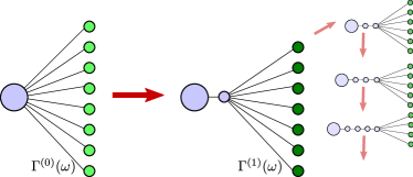
A schematic of the reaction coordinate mapping is shown in Fig. 1. Formally, such mappings can be realized as Bogoliubov transforms, whereby bosonic (or fermionic) annihilation operators are linearly transformed to new bosonic (or fermionic) modes . The reaction coordinate is then selected as one of these new modes :
| (1) |
To preserve the bosonic (fermionic anti-) commutation relations, the Bogoliubov transform needs to be symplectic, i.e., the matrices formed by the complex-valued coefficients and have to obey the relations and , where the sign accounts for bosons and the sign for fermions, respectively. For example, when the transform does not mix creation and annihilation operators (), just needs to be a unitary matrix. As another example, one can construct a bosonic symplectic transform which mixes between annihilation and creation operators from a given orthogonal transform via and where and are real parameters and the orthogonality relation just imposes the constraint . In general, there is an infinite number of such transformations, and we are interested in the ones giving rise to special mappings between Hamiltonians as considered below.
II.1 Spectral bounds
Many generic bosonic Hamiltonians are specifically designed for the weak-coupling limit. When these are naively extrapolated towards strong couplings, it may happen that the spectrum of the complete system is no longer bounded from below, leading to unphysical artifacts. This problem can be circumvented by writing the initial Hamiltonian as a sum of positive definite terms, which upon expansion leads to a renormalized system Hamiltonian. In our considerations below, we will assume that a decomposition of the total Hamiltonian into completed squares has initially been performed, such that the spectrum is always bounded from below for any value of the coupling strength.
II.2 Mappings for continuous bosonic reservoirs
II.2.1 Phonon Mapping
We would like to obtain a map satisfying
| (2) |
where denotes a dimensionless operator acting in the system Hilbert space only, which need not necessarily be bosonic. We term this the phonon mapping due to the position-like couplings both before and after the transformation Woods et al. (2014). In the second line the symbol indicates that the mapped reservoir terms contain one less mode (we may not consistently use this in the following, as the number of modes should become clear from the context). We further note that we have chosen , as a possible phase can be absorbed into the and operators, eventually only leading to a phase in the coefficients. With the same argument, we can choose the coefficients to be real-valued from the beginning. We follow the conventions of defining the corresponding spectral (coupling) densities as
| (3) |
In our units, these have dimensions of energy.
In terms of Bogoliubov transforms, the mapping (II.2.1) can be realized with a normal-mode transformation, where
| (4) |
with real-valued orthogonal matrix , and where the are the natural frequencies of the original modes and the the energies of the transformed modes; specifically is the reaction coordinate energy. Some algebra shows that the first column of the orthogonal matrix is fixed by the original system-reservoir coupling . With this, one obtains the new coupling strength from the old spectral density via
| (5) |
where the energy of the reaction coordinate is determined by
| (6) |
such that both and have dimensions of energy, see Refs. Martinazzo et al. (2011); Strasberg et al. (2016) (note the different factor of two in the definition of the spectral densities).
With the mapping (II.2.1), manipulations on the Heisenberg equations of motion (see Appendix A) tell us that under appropriate conditions the transformed spectral density can be obtained from the old one by the following transformation:
| (7) |
where denotes the Cauchy principal value, and we see that also has units of energy. In this relation, the analytic continuation of the spectral density to the complete real axis is understood. This is again compatible with previous discussions Martinazzo et al. (2011) when the factor of two in the definition of the spectral densities and the correct dimensionality of coupling coefficients in each representation are taken into account. Further, the mapping can be applied recursively, e.g. in the next step we have , and its convergence properties have been thoroughly investigated Martinazzo et al. (2011); Woods et al. (2014). It is straightforward to see that when rescaling with some dimensionless constant , we will just modify the transformed system-reaction coordinate coupling , but the residual spectral density will remain unaffected. This already tells us that the method can be used to explore the strong-coupling limit of extremely large whenever the residual coupling is small. We furthermore see that the spectrum of the supersystem Hamiltonian is bounded from below for any value of when one can decompose , where is bounded from below.
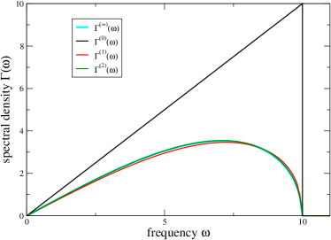
In Table 1 we summarize a few spectral densities for which an analytic computation of the mapping relations according to Eqs. (5), (6), and (7) is possible. One can see that without a rigid cutoff, one may soon obtain spectral densities that do not decay fast enough to allow for another recursive mapping. With a rigid cutoff, we can however observe convergence towards a stationary Rubin-type spectral density as in the bottom right of Table 1, see also Fig. 2 (left panel).
 |
 |
II.2.2 Particle mapping
In analogy with the phonon mapping case, we let the particle mapping be given by
| (8) |
Here, is again some dimensionless system operator, which need not necessarily be Hermitian, and it suffices to choose the Bogoliubov transform as unitary (), see also Ref. Woods et al. (2014) for examples. Then, from identifying and demanding bosonic commutation relations, we must have
| (9) |
Second, we see that the relations together with the unitarity relation fix the first coefficients , which when inserted into the energy of the reaction coordinate eventually yields
| (10) |
such that also has dimensions of energy.
The Heisenberg equations (see Appendix B) tell us that the following spectral density mapping relation should hold
| (11) |
Here, the difference to the phonon mapping is that are not analytically continued to the complete real axis, as is assumed throughout. The convergence properties of related recursion relations have been discussed in great detail Woods et al. (2014, 2015); Woods and Plenio (2016).
As with the previous treatment, the structure of the Hamiltonian (bosonic tunneling) is similar before and after the transformation, we just need to redefine the system and reservoir. Therefore, it can also be applied recursively. This way, we can understand the reaction coordinate mapping as the sequential application of multiple Bogoliubov transformations. In practise, one would truncate the resulting chain at some point, using a perturbative approach such as the master equation Iles-Smith et al. (2014, 2016).
Now, the spectrum of the supersystem Hamiltonian is bounded from below for any value of when one can decompose it as , where is bounded from below. We finally note that by choosing we can switch from a phonon-type representation to a particle-type representation.
II.3 Fermionic particle mapping
We can also investigate these problems for fermions, where the mapping reads
| (12) |
The difference is that the spectral densities can be defined also for negative frequencies, such that no analytic continuation is necessary. Now, we obtain the reaction coordinate coupling and energy from integrals over the complete energies
| (13) |
The Heisenberg equations (see Appendix C) tell us that the following mapping relations should hold
| (14) |
where we again stress that the spectral density is defined also for negative energies. When we consider the case that it strictly vanishes for negative energies, we recover the case of bosonic particle mappings from Eqs. (9), (10), and (11).
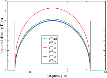
Table 2 provides some examples of spectral densities and their mappings according to Eqs. (13) and (14). The functional form of the mapping implies that convergence of all integrals is ensured only for a hard cutoff. In particular, the limiting case for particle mappings with a rigid cutoff is a semicircle, see the bottom right entry in Table 2, which we also observe numerically in Fig. 2 (right panel).
II.4 General Properties: Stationary state of the supersystem
In the strong-coupling limit, we no longer expect the local Gibbs state to be the stationary state of the system. Rather, one might expect it to be given by the reduced density matrix of the total Gibbs state Gogolin and Eisert (2016); Perarnau-Llobet et al. (2018)
| (15) |
which would only coincide with the system-local Gibbs state when (vanishingly weak coupling). Since the reaction coordinate mappings allow for arbitrarily strong coupling between the original system and reservoir, we can test when the resulting stationary state in the supersystem is consistent with these expectations.
In particular, we assume here that the coupling between the supersystem and residual reservoir is small, such that we can apply the master equation formalism to the supersystem Iles-Smith et al. (2014, 2016)
| (16) |
composed of system and reaction coordinate. For the standard quantum-optical master equation (based in general on Born-Markov and secular approximations) it is known that for a single reservoir the stationary state will approach the system-local Gibbs state Dümcke and Spohn (1979); Breuer and Petruccione (2002), now associated with the supersystem Iles-Smith et al. (2014)
| (17) |
We define a Hamiltonian of mean force – see also the previous chapter –via the relation
| (18) |
It can be seen as an effective Hamiltonian for the system in the strong coupling limit. In the weak-coupling limit () we get . By construction, the Hamiltonian of mean force obeys
| (19) |
Here, serves as a dimensionless bookkeeping parameter for the coupling between the reaction coordinate and the residual reservoir. With Eq. (17), this implies that the reduced steady state of the original system becomes
| (20) |
where the last equality follows directly from performing . That is, when the coupling between the supersystem and the residual reservoir (i.e. the transformed spectral density) is small, the approach recovers the reduced steady state (15) of the global Gibbs state Iles-Smith et al. (2014); Strasberg et al. (2016).
III Applications to thermal machines
Heat engines generate useful work by harnessing heat flow between hot and cold reservoirs. Usually, heat engine models are analysed under the simplifying assumption of negligibly weak interactions between the working system and the reservoirs. However, as argued earlier, for heat engines operating at the quantum scale such an approximation may not be well justified, since interaction energies potentially become comparable with system and reservoir self-energy scales. The treatment becomes even more challenging when one allows for driven heat engines, where the coupling strength between the system and reservoir is modified periodically. In such cases, even the correct partition of the time-dependent system-reservoir driving into heat and work contributions is generally a challenging task, where the reaction coordinate treatment is indeed helpful Restrepo et al. (2018). For conceptual simplicity, however, we shall put the simultaneous treatment of driving and dissipation aside and therefore review two types of heat engine model in this section – discrete stroke and continuous – that have recently been analysed beyond weak system-reservoir coupling by employing the reaction coordinate formalism outlined above.
III.1 Discrete stroke engines: the Otto cycle
Discrete stroke heat engines operate in closed cycles that are divided into individual sections (strokes) in which particular operations such as heat exchange, expansion, compression, or combinations, take place. The working system returns to its original state at the end of the cycle and in order to produce a finite power output, each stroke must be performed within a finite time. Nevertheless, the study of infinite time cycles (which produce work but zero power output) has been crucial in identifying fundamental thermodynamic bounds on heat engine performance, and indeed led to Carnot’s principle. Furthermore, the identification of a closed cycle is made easier in the infinite time limit due to the knowledge of the state (whether within the weak-coupling or reaction coordinate approaches) after equilibration between the system and the hot or cold reservoir. Thus, zero power cycles provide a natural setting in which to begin exploring extensions of heat engine models beyond the weak system-reservoir coupling regime.
Here we shall review the reaction coordinate analysis of a discrete stroke quantum Otto cycle beyond weak reservoir coupling as presented in Ref. Newman et al. (2017). This cycle is a quantum analogy of a four-stroke internal combustion engine model. It has the advantage of separating strokes in which energy is exchanged between the system and the reservoirs from those in which work is either extracted from or done on the system with the reservoirs uncoupled. In this way, we seek to avoid the complications of defining work and heat at strong-coupling for strokes in which both may be important, as encountered for example within the Carnot cycle.
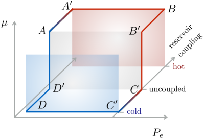
The strokes of our quantum Otto cycle are depicted schematically in Fig. 3. We consider a two-level working system with ground state and excited state , split by an energy . The system may be coupled to and decoupled from two reservoirs, one hot and one cold. In the standard approach assuming negligibly weak system-reservoir interactions these coupling and decoupling steps make no energetic contribution to the cycle. This can be seen, for example, if we consider the system to couple linearly to bosonic reservoirs that remain in thermal equilibrium (factorised from the system state) throughout the cycle, in which case the trace of the interaction Hamiltonian evaluates to zero. Under these conditions, the Otto cycle consists of four strokes, two isentropes in which the system Hamiltonian is varied in time in the absence of any reservoir coupling, and two isochores in which the system equilibrates with either the hot or cold reservoir without any variations in the system Hamiltonian. However, for the case of finite reservoir coupling that is of interest here, there is no reason to believe that the coupling and decoupling steps can be neglected. We must therefore enlarge the cycle to include these contributions as well, leading to the primed points in Fig. 3.
Let us now analyse the cycle in more detail, contrasting the reaction coordinate and weakly-interacting approaches. Starting, arbitrarily, at point in Fig. 3, the system and hot reservoir have just been coupled. They are allowed to equilibrate along the subsequent stroke, known as the hot isochore, which means that within the weak-coupling limit the state of the system plus hot reservoir is given at point by
| (21) |
Here, is the inverse temperature of the hot reservoir with internal Hamiltonian . For weak coupling, the system simply thermalises along the stroke with respect to its internal Hamiltonian . The system-reservoir coupling strength thus plays no role in the infinite time weak-coupling limit. In contrast, within the reaction coordinate formalism the state at the end of the stroke is given by
| (22) |
where is now a Gibbs (thermal) state of the supersystem comprised of both the original two-level system and the reaction coordinate, as defined in Eq. (17) with . This encodes correlations due to finite interactions between the system and reservoir, and thus has a natural dependence on the system-reservoir coupling strength as well as the reservoir temperature. Note that the factorisation in Eq. (22) is made only with respect to the mapped residual bath with internal Hamiltonian , given for example by the final terms in Eqs. (II.2.1) and (II.2.2). It is not, therefore, equivalent to a weak-coupling approximation between the system and the full reservoir as in Eq. (21). Accordingly, numerical benchmarking of the reaction coordinate method has shown it to be accurate over a very wide range of system-environment coupling strengths Iles-Smith et al. (2014, 2016).
The quantity of interest for analysing the cycle performance is the energy expectation value at the end of each stroke. In the weak coupling limit only changes to the two-level system energy are tracked, and so we consider
| (23) |
In the reaction coordinate approach, on the other hand, changes to both the system and reaction coordinate are monitored, and so we have
| (24) |
which includes additional contributions from the reaction coordinate and system-reaction coordinate Hamiltonians through , as well as correlation effects through .111Note that there is a subtlety in the strong-coupling cycle. When coupled, the interaction between the system and the reservoir pushes the latter out of thermal equilibrium. We assume that once the system and reservoir are decoupled at the end of the stroke, the reservoir rapidly relaxes back to equilibrium. Hence, when the system comes to be coupled to the reservoir again on the next cycle, the reservoir is thermal once more. The re-thermalisation of the reservoirs entails accounting for some extra energetic contributions around the cycle, as described in detail in Newman et al. (2017).
At point the interaction between the system and hot reservoir is now turned off to reach point , which we must explicitly account for within the reaction coordinate analysis. For simplicity we shall assume this happens suddenly, such that the full state does not change, and hence define a work cost associated with decoupling of
| (25) |
This cost impacts adversely on the total work output of the cycle. In Ref. Newman et al. (2017) it is shown that part (though not all) of the work cost can be mitigated by decoupling the system and reservoir slowly (i.e. in the adiabatic limit), see also Fig. 4.
From point to the system Hamiltonian is changed such that the splitting is reduced () in the absence of any reservoir coupling, with the stroke thus being termed isentropic expansion. For changes that are slow enough to justify use of the quantum adiabatic theorem, the average system energy along the stroke is given simply by
| (26) |
where refers to the start of the stroke, in the weak-coupling case, and in the reaction coordinate treatment. Thus, the work output of the stroke becomes
| (27) |
which is negative by convention.
The coupling to the cold reservoir is now switched on (). We assume the reservoirs relax back to thermal equilibrium when decoupled from the system, and so there is no work contribution associated with this step in either treatment as the trace of the interaction Hamiltonian is then zero. The system and cold reservoir now equilibrate along the subsequent stroke (), which we may analyse in the same way as the hot isochore. They are then decoupled () once more incurring a work cost in the reaction coordinate treatment. Subsequently, we do work on the system during an isentropic compression (). Here, the system splitting is adiabatically increased back to its earlier value, such that . Finally, the system and hot reservoir are coupled (, no work cost) and the cycle is complete.
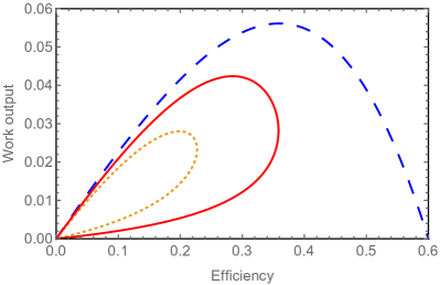
In Fig. 4 we show some example parametric plots of the efficiency and work output of the Otto cycle as treated within both the weak-coupling and reaction coordinate frameworks. To generate these curves the difference in splittings between the start and end of the isentropic stokes is varied. In the weak-coupling case, the net work output is simply the difference in work along the two isentropic strokes, whereas in the reaction coordinate treatment we must include the decoupling costs as well. In both cases, we define the efficiency in the standard way as
| (28) |
where is the cycle net work output and is the energy change along the hot isochore. For the weak-coupling case this can be expressed in the simple form , which depends only on the ratio of the two-level splittings. We can see from Fig. 4 that the weak-coupling efficiency reaches a maximum at the point at which the work output vanishes. Here, the ratio of splittings becomes equal to the ratio of cold to hot reservoir temperatures, , and so the weak-coupling efficiency reaches the Carnot bound. The behaviour of the cycle is qualitatively different, and inferior, in the reaction coordinate case. The maximum efficiency occurs at finite work output, though takes values well below the Carnot bound, and the efficiency also falls to zero as the work output vanishes at larger ratios of the two-level splittings. The decoupling cost contributions are the primary cause for the reduced engine performance at strong-coupling, with a small reduction in energy absorbed along the hot isochore insufficient to overcome their detrimental effect to the efficiency Newman et al. (2017). Finally, we note that an adiabatic decoupling protocol can improve both efficiency and work output (though not up to the idealised weak-coupling limit), and should thus be an important consideration in optimising the performance of nanoscale (quantum) engine cycles where the presence of non-negligible reservoir couplings is expected Le Hur (2012); Goldstein et al. (2013); Peropadre et al. (2013); Nazir and McCutcheon (2016).
III.2 Continuously operating thermo-machines
For continuously operating heat engines (or refrigerators), the system of interest is coupled to multiple reservoirs that are held at different local thermal equilibrium states throughout Kosloff and Levy (2014). It is then possible to use, for example, a thermal gradient between the reservoirs to extract (chemical) work by transporting electrons against a bias (heat engine) or to cool the coldest reservoir by investing work (chemical work or the energy provided by a so-called work reservoir). In this section, we shall exemplarily benchmark the reaction coordinate treatment of an exactly-solvable two-terminal model.
The single-electron transistor (SET) with Hamiltonian
| (29) |
describes a single quantum dot with on-site energy that is coupled via tunneling amplitudes to two fermionic leads . Letting the leads become continuous, we introduce the original lead spectral densities . The model can be analyzed as a heat engine with a perturbative treatment of the Esposito et al. (2009). However, an exact solution can also be derived Haug and Jauho (2008) and analyzed from a thermodynamic viewpoint Topp et al. (2015). We consider reservoirs described by temperatures and chemical potentials and use conservation of energy and matter currents at steady state throughout.
One observable of interest is then the chemical work rate extracted from the system
| (30) |
where denotes the electronic matter current counting positive from left to right. For , this process can be interpreted as electric power used to transport electrons against a bias voltage . Furthermore, we define the stationary heat currents entering the system as
| (31) |
where denotes the energy current counting positive from left to right. Without loss of generality, we consider setups where and (). Then, the efficiency of generating electric power from the heat coming from the hot reservoir becomes
| (32) |
where denotes the Heaviside- function. Here, the upper bound by Carnot efficiency follows from the positivity of the entropy production rate, which at steady state reduces to Topp et al. (2015). With the same argument, the coefficient of performance for cooling the cold reservoir by investing chemical work ,
| (33) |
must also obey a Carnot bound.
We can exactly evaluate energy and matter currents for the SET model using for example nonequilibrium Green’s function techniques Haug and Jauho (2008); Bruch et al. (2016) or other approaches Topp et al. (2015), which eventually allows for an exact evaluation of heat engine efficiency (32) and COP (33) for arbitrary system-reservoir coupling strengths. Alternatively, we can apply the fermionic reaction coordinate mapping Strasberg et al. (2018), which – when we use a separate reaction coordinate for every reservoir – transforms the SET to a triple quantum dot that is tunnel-coupled to two residual leads Schaller et al. (2018)
| (34) |
where we have reaction coordinate couplings and energies as well as a new spectral density . Specifically, using the Lorentzian spectral density from the first row of Table 2 centred around with coupling strengths and width , we see that the resulting triple quantum dot is tunnel-coupled to two residual reservoirs with a flat spectral density, to which a Markovian treatment of the supersystem (first three terms in the above equation) should apply when is small. For this supersystem, we can set up the (non-secular) master equation (compare with Ref. Schaller et al. (2018) in absence of feedback control operations) and compute energy and matter currents entering the supersystem from the residual reservoirs. At steady state, we can identify these with the original currents defined above (the reaction coordinates can only host finite charge/energy) and therefore likewise evaluate heat engine efficiency and COP within the reaction coordinate formalism. The result of this procedure is depicted in Fig. 5 (left panel).
There we see that at vanishing coupling, where the conventional single dot master equation approach to the SET applies Esposito et al. (2009), maximal efficiencies are actually reached (albeit at zero power or cooling current, respectively), and the transition between heat engine and cooling operational modes happens directly. This can be understood since in the limit of vanishing coupling, the SET obeys the so-called tight-coupling condition . For finite coupling strengths , a gap between these modes opens, which is also observed in other models beyond the weak-coupling limit Restrepo et al. (2018). When we further increase the coupling strength, the cooling function is no longer attainable, and also the efficiency of the heat engine decreases. Most importantly, we see that the reaction coordinate treatment (dashed contours), reproduces the exact solution (colours and solid green contours) well, which is attributable to the fact that we choose initially highly peaked spectral densities, such that the residual coupling is very small and the reaction coordinate treatment is valid.
One might now be tempted to think that larger coupling strengths are always detrimental to the perfomance of thermoelectric devices, compare Ref. Perarnau-Llobet et al. (2018) or the discussion in the previous subsection. With the exact solution at hand, there is little intuitive evidence for finding other interesting parameter regimes. However, going further towards ultra-strong coupling reveals that there is a regime where the heat engine efficiency increases again, and even the cooling operational mode is revived, as is illustrated in Fig. 5 (right panel). From comparing the contours we can see that the reaction coordinate treatment (dashed) correctly predicts the revival of the cooling mode and the strengthening of the heat engine efficiency in this limit. We note that as the tunnel amplitudes scale only with the root of the coupling strength for the parameters in Fig. 5, this regime is actually not unrealistic, as has been experimentally demonstrated in various quantum dot systems Baines et al. (2012); Hensgens et al. (2017); Bayer et al. (2017). From the experimental side, the challenge is rather the maintenance of a thermal gradient.
Within the reaction coordinate picture, this worsening and re-strengthening of performance can be understood with a simple transport spectroscopy interpretation. It is rather straightforward to diagonalize the supersystem Hamiltonian in the first three terms of Eq. (34). Between the 8 energy eigenstates of the supersystem, not all transitions are allowed in the sequential tunneling regime, see Fig. 6.
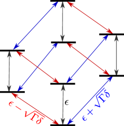
Adopting equal coupling strengths and widths for both reservoirs, and matching the maximum tunneling rate with that of the central dot , the allowed transition frequencies simplify to
| (35) |
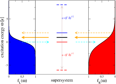
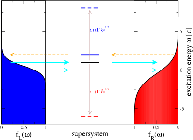
With modifying the coupling strength , we therefore change the transition energies as well. For vanishingly small coupling strengths , the splitting is not resolved by the rather large reservoir temperatures as , and the only visible transition frequency is . As mentioned, in this regime the setup approximately obeys the tight-coupling property , and maximum efficiencies are reached (albeit at vanishing power) den Broeck (2005); Gomez-Marin and Sancho (2006); Sheng and Tu (2013). Here, even the naive (weak-coupling) SET master equation treatment is valid. When we increase the coupling strength, we leave the tight-coupling regime, i.e. energy and matter currents are no longer proportional to each other, which is known to decrease efficiencies, eventually even leading to the loss of the cooling function. However, when , , and , the two shifted excitation energies will have left the transport window and will no longer participate in transport. Then, tight coupling is again restored as only one transition energy remains inside the transport window. We illustrate this in Fig. 7.
 |
 |
Beyond a benchmark of the reaction coordinate treatment, this example provides a simple explanation of the observed behaviour and demonstrates that the mapping can be used as a tool to identify interesting parameter regimes, allowing for useful operational modes. Strong coupling is not always detrimental to the efficiency of continuous heat engines. However, regarding overall power output, it should be noted that we had to choose small (highly structured reservoirs) to maintain the validity of the reaction coordinate treatment. This does of course bound the total power output of the device, which is not proportional to the coupling strength in this regime.
IV Outlook
The reaction coordinate mapping is typically used to explore the strong-coupling regime, and as such it has found widespread application. We stress here that it may also be extended to fermionic reservoirs. By construction, the mapping itself is exact and thus barely suffers from additional constraints. It can also be combined, for example, with formally exact methods such as nonequilibrium Green’s functions Haug and Jauho (2008), to simplify the structure of the resulting equations. However, when it is combined with some perturbative technique, its applicability will be limited to a certain degree. For example, to apply a master equation to the supersystem, it is required that the residual (mapped) spectral density allows for a Markovian treatment. Thus, the master equation solution obtained via the reaction coordinate mapping will in general have a different range of validity than the master equation solution of the original system Iles-Smith et al. (2014, 2016). We further note that with the mapping, one can transfer the time-dependence of parameters into the supersystem, thus enabling the treatment of open-loop control schemes such as periodic driving Restrepo et al. (2018), or feedback control schemes such as Maxwell’s demon Schaller et al. (2018), from the perspective of a driven system only.
The intuitive simplicity of the reaction coordinate technique makes it suitable to extend the range of validity of many different perturbative approaches. Indeed, beyond strong coupling, other problems can be treated with reaction coordinate mappings. For example, with the mapping one can study the effect of initial system-reservoir correlations by means of master equations. Furthermore, as the treatment of the supersystem is Markovian, but the reduced dynamics of the original need not be, one can see the reaction coordinate mapping as a Markovian embedding to study non-Markovian dynamics.
Finally, we mention that one can also use the mapping to engineer structured reservoirs. Equipping a quantum system of interest with auxiliary degrees of freedom, which are coupled to structureless reservoirs, we can interpret the auxiliary degrees of freedom as reaction coordinates and perform the inverse mapping. Eventually, this yields a system coupled to structured reservoirs, with reaction coordinates that can for example be used as frequency filters to optimize performance of heat engines or other devices.
V Acknowledgments
G.S. gratefully acknowledges discussions with J. Cerrillo, N. Martensen, S. Restrepo, and P. Strasberg and financial support by the DFG (GRK 1558, SFB 910, SCHA 1646/3-1, BR 1528/9-1).
A.N. would like to thank D. Newman, F. Mintert, J. Iles-Smith, N. Lambert, Z. Blunden-Codd and V. Jouffrey for discussions. A.N. is supported by the Engineering and Physical Sciences Research Council, grant no. EP/N008154/1.
References
- Liu et al. (2007) Y. Liu, Y. Zheng, W. Gong, W. Gao, and T. Lü, Physics Letters A 365, 495 (2007).
- Nesi et al. (2007) F. Nesi, E. Paladino, M. Thorwart, and M. Grifoni, Europhysics Letters 80, 40005 (2007).
- Hörhammer and Büttner (2008) C. Hörhammer and H. Büttner, Journal of Statistical Physics 133, 1161 (2008).
- Campisi et al. (2009) M. Campisi, P. Talkner, and P. Hänggi, Phys. Rev. Lett. 102, 210401 (2009).
- Nicolin and Segal (2011) L. Nicolin and D. Segal, Physical Review B 84, 161414 (2011).
- Deffner and Lutz (2011) S. Deffner and E. Lutz, Phys. Rev. Lett. 107, 140404 (2011).
- Hausinger and Grifoni (2011) J. Hausinger and M. Grifoni, Physical Review A 83, 030301 (2011).
- Pucci et al. (2013) L. Pucci, M. Esposito, and L. Peliti, Journal of Statistical Mechanics: Theory and Experiment 2013, P04005 (2013).
- Schaller et al. (2013) G. Schaller, T. Krause, T. Brandes, and M. Esposito, New Journal of Physics 15, 033032 (2013).
- Ankerhold and Pekola (2014) J. Ankerhold and J. P. Pekola, Phys. Rev. B 90, 075421 (2014).
- Iles-Smith et al. (2014) J. Iles-Smith, N. Lambert, and A. Nazir, Physical Review A 90, 032114 (2014).
- Gallego et al. (2014) R. Gallego, A. Riera, and J. Eisert, New Journal of Physics 16, 125009 (2014).
- Wang et al. (2015) C. Wang, J. Ren, and J. Cao, Scientific Reports 5, 11787 (2015).
- Esposito et al. (2015a) M. Esposito, M. A. Ochoa, and M. Galperin, Phys. Rev. Lett. 114, 080602 (2015a).
- Esposito et al. (2015b) M. Esposito, M. A. Ochoa, and M. Galperin, Physical Review B 92, 235440 (2015b).
- Gelbwaser-Klimovsky and Aspuru-Guzik (2015) D. Gelbwaser-Klimovsky and A. Aspuru-Guzik, The Journal of Physical Chemistry Letters 6, 3477 (2015).
- Carrega et al. (2015) M. Carrega, P. Solinas, A. Braggio, M. Sassetti, and U. Weiss, New Journal of Physics 17, 045030 (2015).
- Strasberg et al. (2016) P. Strasberg, G. Schaller, N. Lambert, and T. Brandes, New Journal of Physics 18, 073007 (2016).
- Katz and Kosloff (2016) G. Katz and R. Kosloff, Entropy 18, 186 (2016).
- Cerrillo et al. (2016) J. Cerrillo, M. Buser, and T. Brandes, Physical Review B 94, 214308 (2016).
- Seifert (2016) U. Seifert, Phys. Rev. Lett. 116, 020601 (2016).
- Newman et al. (2017) D. Newman, F. Mintert, and A. Nazir, Physical Review E 95, 032139 (2017).
- Strasberg and Esposito (2017) P. Strasberg and M. Esposito, Physical Review E 95, 062101 (2017).
- Miller and Anders (2017) H. J. D. Miller and J. Anders, Phys. Rev. E 95, 062123 (2017).
- Mu et al. (2017) A. Mu, B. K. Agarwalla, G. Schaller, and D. Segal, New Journal of Physics 19, 123034 (2017).
- Jarzynski (2017) C. Jarzynski, Phys. Rev. X 7, 011008 (2017).
- Freitas and Paz (2017) N. Freitas and J. P. Paz, Phys. Rev. E 95, 012146 (2017).
- Perarnau-Llobet et al. (2018) M. Perarnau-Llobet, H. Wilming, A. Riera, R. Gallego, and J. Eisert, Phys. Rev. Lett. 120, 120602 (2018).
- Burkey and Cantrell (1984) R. S. Burkey and C. D. Cantrell, Journal of the Optical Society of America B 1, 169 (1984).
- Garg et al. (1985) A. Garg, J. N. Onuchic, and V. Ambegaokar, The Journal of Chemical Physics 83, 4491 (1985).
- Martinazzo et al. (2011) R. Martinazzo, B. Vacchini, K. H. Hughes, and I. Burghardt, The Journal of Chemical Physics 134, 011101 (2011).
- Woods et al. (2014) M. P. Woods, R. Groux, A. W. Chin, S. F. Huelga, and M. B. Plenio, Journal of Mathematical Physics 55, 032101 (2014).
- Schaller et al. (2018) G. Schaller, J. Cerrillo, G. Engelhardt, and P. Strasberg, Phys. Rev. B 97, 195104 (2018).
- Strasberg et al. (2018) P. Strasberg, G. Schaller, T. L. Schmidt, and M. Esposito, Phys. Rev. B 97, 205405 (2018).
- Restrepo et al. (2018) S. Restrepo, J. Cerrillo, P. Strasberg, and G. Schaller, New Journal of Physics doi:10.1088/1367-2630/aac583 (2018), 10.1088/1367-2630/aac583.
- Iles-Smith et al. (2016) J. Iles-Smith, A. G. Dijkstra, N. Lambert, and A. Nazir, The Journal of Chemical Physics 144, 044110 (2016).
- Huh et al. (2014) J. Huh, S. Mostame, T. Fujita, M.-H. Yung, and A. Aspuru-Guzik, New Journal of Physics 16, 123008 (2014).
- Woods et al. (2015) M. P. Woods, M. Cramer, and M. B. Plenio, Physical Review Letters 115, 130401 (2015).
- Woods and Plenio (2016) M. P. Woods and M. B. Plenio, Journal of Mathematical Physics 57, 022105 (2016).
- Gogolin and Eisert (2016) C. Gogolin and J. Eisert, Reports on Progress in Physics 79, 056001 (2016).
- Dümcke and Spohn (1979) R. Dümcke and H. Spohn, Zeitschrift für Physik B 34, 419 (1979).
- Breuer and Petruccione (2002) H.-P. Breuer and F. Petruccione, The Theory of Open Quantum Systems (Oxford University Press, Oxford, 2002).
- Le Hur (2012) K. Le Hur, Phys. Rev. B 85, 140506 (2012).
- Goldstein et al. (2013) M. Goldstein, M. H. Devoret, M. Houzet, and L. I. Glazman, Phys. Rev. Lett. 110, 017002 (2013).
- Peropadre et al. (2013) B. Peropadre, D. Zueco, D. Porras, and J. J. García-Ripoll, Phys. Rev. Lett. 111, 243602 (2013).
- Nazir and McCutcheon (2016) A. Nazir and D. P. S. McCutcheon, Journal of Physics: Condensed Matter 28, 103002 (2016).
- Kosloff and Levy (2014) R. Kosloff and A. Levy, Annual Review of Physical Chemistry 65, 365 (2014).
- Esposito et al. (2009) M. Esposito, K. Lindenberg, and C. V. den Broeck, Europhysics Letters 85, 60010 (2009).
- Haug and Jauho (2008) H. Haug and A.-P. Jauho, Quantum Kinetics in Transport and Optics of Semiconductors (Springer, 2008).
- Topp et al. (2015) G. E. Topp, T. Brandes, and G. Schaller, Europhysics Letters 110, 67003 (2015).
- Bruch et al. (2016) A. Bruch, M. Thomas, S. Viola Kusminskiy, F. von Oppen, and A. Nitzan, Phys. Rev. B 93, 115318 (2016).
- Baines et al. (2012) D. Y. Baines, T. Meunier, D. Mailly, A. D. Wieck, C. Bäuerle, L. Saminadayar, P. S. Cornaglia, G. Usaj, C. A. Balseiro, and D. Feinberg, Phys. Rev. B 85, 195117 (2012).
- Hensgens et al. (2017) T. Hensgens, T. Fujita, L. Janssen, X. Li, C. J. V. Diepen, C. Reichl, W. Wegscheider, S. D. Sarma, and L. M. K. Vandersypen, Nature 548, 70 (2017).
- Bayer et al. (2017) J. C. Bayer, T. Wagner, E. P. Rugeramigabo, and R. J. Haug, Phys. Rev. B 96, 235305 (2017).
- den Broeck (2005) C. V. den Broeck, Physical Review Letters 95, 190602 (2005).
- Gomez-Marin and Sancho (2006) A. Gomez-Marin and J. M. Sancho, Phys. Rev. E 74, 062102 (2006).
- Sheng and Tu (2013) S. Sheng and Z. C. Tu, Journal of Physics A: Mathematical and Theoretical 46, 402001 (2013).
Appendix A Heisenberg equations for the phonon mapping
The Heisenberg equations of motion for a system observable read in the original representation
| (36) |
We now Fourier-transform these equations according to with the convention . In -space, the creation and annihilation operators are no longer adjoint to each other, but we will keep the -notation. This yields the algebraic equations (convolution theorem)
| (37) |
We can solve the last two equations and , and insert them into the first
| (38) |
Here, we have in the first step used the fact that the harmonic oscillator frequencies are by construction all positive and we have introduced the Cauchy transform
| (39) |
where the last equality sign holds for analytic continuation as an odd function . In particular, we note the important property
| (40) |
Similarly, we can derive the Heisenberg equations of motion in the mapped representation, and Fourier-transform them according to the same prescription, yielding
| (41) |
Again, we follow the approach of successively eliminating the , , and then the , variables, yielding for the remaining equation
| (42) |
Comparing this with the original representation, we can infer a relation between and , which can be used to obtain the transformed spectral density
| (43) |
Appendix B Heisenberg equations for the particle mapping
Now, the Heisenberg equations of motion for a system observable read in the original representation
| (44) |
Fourier-transformation yields
| (45) |
Inserting the solutions of the last two equations into the first we get
| (46) |
In the mapped representation, we have
| (47) |
such that Fourier transformation yields
| (48) |
Successive elimination of the last four equations yields for the remaining one
| (49) | ||||
From comparison with the first representation, we conclude
| (50) |
where the second equation just encodes the first at and is therefore not independent.
From realizing that
| (51) |
we can use e.g. the first of these relations to infer a mapping relation between the spectral densities,
| (52) |
where is assumed throughout.
Appendix C Heisenberg equations for fermionic reservoirs
To avoid case distinctions on whether the system operator commutes or anti-commutes with the coupling operator, we just consider the Heisenberg equations for the creation and annihilation operators. In the original representation, they become
| (53) |
and similarly for the creation operators. Since at this level they do not mix, we consider only the annihilation operators. Fourier-transformation yields
| (54) |
Eliminating the second equation then gives
| (55) |
In contrast, the mapped representation yields
| (56) |
Fourier-transforming and eliminating the non-system variables then gives
| (57) |
and from comparison we get the relation
| (58) |
Converting the sums to integrals and evaluating at when we obtain a mapping relation between the fermionic spectral densities:
| (59) |