Anchored Bayesian Gaussian Mixture Models

Deborah Kunkel¹ and Mario Peruggia²

1. School of Mathematical and Statistical Sciences, Clemson University, Clemson, SC, USA
2. Department of Statistics, The Ohio State University, Columbus, OH, USA

Abstract

Finite mixtures are a flexible modeling tool for irregularly shaped densities and samples from heterogeneous populations. When modeling with mixtures using an exchangeable prior on the component features, the component labels are arbitrary and are indistinguishable in posterior analysis. This makes it impossible to attribute any meaningful interpretation to the marginal posterior distributions of the component features. We propose a model in which a small number of observations are assumed to arise from some of the labeled component densities. The resulting model is not exchangeable, allowing inference on the component features without post-processing. Our method assigns meaning to the component labels at the modeling stage and can be justified as a data-dependent informative prior on the labelings. We show that our method produces interpretable results, often (but not always) similar to those resulting from relabeling algorithms, with the added benefit that the marginal inferences originate directly from a well specified probability model rather than a post hoc manipulation. We provide asymptotic results leading to practical guidelines for model selection that are motivated by maximizing prior information about the class labels and demonstrate our method on real and simulated data.

1 Introduction

Finite mixture models are flexible tools that are often applied to data from heterogeneous populations or from distributions with irregularly-shaped densities. In these context, they can produce useful approximations to the unknown density functions in both univariate and multivariate settings (Frühwirth-Schnatter,, 2006; Marin and Robert,, 2014; Rossi,, 2014). Results concerning the accuracy and consistency of the approximations (as the number of components increases at an appropriate rate) have been established both in the frequentist and in the Bayesian settings (Roeder and Wasserman,, 1997; Genovese and Wasserman,, 2000; Norets and Pelenis,, 2012). In many situations, if the true density is well-behaved in the tails, satisfactory approximations can be obtained using a small or moderate number of mixture components.

When mixture distributions are used to model heterogeneous populations, the mixture components are thought to represent clusters of similar units. Such analyses are found in areas such as medicine, the social sciences, and genetics, where identifying subgroups of similar individuals may help to generate hypotheses for future research. When subgroup identification is an important goal, as it is in this paper, the parameters of the component distributions provide population-level information about the features of groups, which can elucidate the overarching patterns of heterogeneity within a population. Therefore, accurate estimates of component-specific parameters, with attendant measures of uncertainty, become a vital element of inference. Further, the mixture model allows estimation of a probabilistic clustering structure from the data.

Adopting standard notation (e.g., Frühwirth-Schnatter,, 2006), we represent the likelihood for a $k$-component finite mixture model for a response $\mbox{\boldmath$y$}=(y_{1},\ldots,y_{n})$ as

$$f(\mbox{\boldmath$y$}|\mbox{\boldmath$\gamma$},\mbox{\boldmath$\eta$}) =\prod_{i=1}^{n}\sum_{j=1}^{k}\eta_{j}p(y_{i}|\gamma_{j}),$$ (1)

where $p(\cdot|\gamma_{j})$ denotes the $j$th component density. The model is parameterized by $\mbox{\boldmath$\eta$}=(\eta_{1},\ldots,\eta_{k})$, the vector of mixture proportions whose elements sum to one, and $\mbox{\boldmath$\gamma$}=(\gamma_{1},\ldots,\gamma_{k})$, the vector of features of the component densities. It is often helpful to write the model (1) hierarchically, using latent variables $\mbox{\boldmath$S$}=\{S_{1},\ldots,S_{n}\}$, $S_{i}\in\{1,\ldots,k\}$, $i=1,\ldots,n$, to indicate component membership. The resulting likelihood is

$$f(\mbox{\boldmath$y$}|\mbox{\boldmath$s$},\mbox{\boldmath$\gamma$}) =\prod_{i=1}^{n}p(y_{i}|\gamma_{s_{i}}),\quad\mbox{where }\;\;\;P(S_{i}=j|\mbox{\boldmath$\eta$})=\eta_{j},\quad j=1,\ldots,k;\quad i=1,\ldots,n.$$ (2)

If the population comprises well-understood groups, it is appropriate to incorporate information regarding the groups’ relative locations and scales into the prior on $(\mbox{\boldmath$\gamma$},\mbox{\boldmath$\eta$})$. Often, however, little is known about these groups ahead of time, and it is natural to assume prior exchangeability of component features. Let $q$ index the $k!$ possible permutations of the integers $1,\ldots,k$ and let $\rho_{q}(\cdot)$ relabel its argument according to the $q$th permutation. We will use the same symbol $\rho_{q}(\cdot)$ to denote the action of the $q$th permutation on a given index between 1 and $k$ and on the elements of a vector argument. For example, if the $q$th permutation of $(1,2,3,4)$ is $(1,3,4,2)$, then $\rho_{q}(3)=4$ and $\rho_{q}(a_{1},a_{2},a_{3},a_{4})=(a_{1},a_{3},a_{4},a_{2})$.

An exchangeable prior with density $\pi$ satisfies $\pi(\mbox{\boldmath$\gamma$},\mbox{\boldmath$\eta$})=\pi(\rho_{q}(\mbox{\boldmath$\gamma$},\mbox{\boldmath$\eta$})),$ $q=1,\ldots,k!$. This specification produces a posterior distribution that inherits the same label invariance; that is, letting $p_{E}(\cdot|\mbox{\boldmath$y$})$ denote the posterior density of $(\mbox{\boldmath$\gamma$},\mbox{\boldmath$\eta$})$ under the exchangeable model,

$$p_{E}(\mbox{\boldmath$\gamma$},\mbox{\boldmath$\eta$}|\mbox{\boldmath$y$}) =p_{E}(\rho_{q}(\mbox{\boldmath$\gamma$},\mbox{\boldmath$\eta$})|\mbox{\boldmath$y$}),\quad q=1,\ldots,k!.$$ (3)

The posterior density is symmetric with respect to the $k!$ labelings of the components, often producing $k!$ modal regions in the parameter space. The marginal distributions of the component-specific parameters are identical. When Markov Chain Monte Carlo methods are used to sample from the posterior distribution of $(\mbox{\boldmath$\gamma$},\mbox{\boldmath$\eta$})$, a well-mixed chain will jump from one possible labeling to another, a phenomenon referred to as “label-switching.”

The posterior symmetry and accompanying label-switching in no way hinders the model’s predictive performance, nor does it preclude meaningful inference on objects that do not depend on the component labels. When label-switching occurs, however, ergodic averages cannot be used for inference on the component-specific features, making it impossible to use labeled parameters to learn about distinctions among the mixture components. Much work has been devoted to either preventing or reversing label-switching by placing prior constraints on the parameter space or by post-processing posterior samples in a way that allows only one possible labeling of the mixture components. These approaches, particularly the post-processing approach, are popular in practice.

Prior identifiability constraints create a non-exchangeable prior by requiring $(\mbox{\boldmath$\gamma$},\mbox{\boldmath$\eta$})$ to lie in some sub-region of the parameter space that is compatible with only one possible labeling. For example, one could require that $\eta_{1}<\ldots<\eta_{k}$ with probability $1$, or establish similar ordering constraints among the component feature parameters. The limitations of these approaches are addressed in detail by, among others, Celeux et al., (2000) and Jasra et al., (2005). They are often considered too informative in their strict restrictions of the parameter space and may not effectively isolate a single modal region of the posterior density. It is not always obvious, a priori, what choice of constraint is appropriate for a problem.

Relabeling algorithms, such as those presented by Stephens, (2000); Celeux et al., (2000); Marin et al., (2005); Papastamoulis and Iliopoulos, (2010); Bardenet et al., (2012); Rodriguez and Walker, (2014), and Li and Fan, (2016), tend to be preferred. These algorithms specify a loss function and find the labeling that minimizes the loss function for each posterior sample of $(\mbox{\boldmath$\gamma$},\mbox{\boldmath$\eta$})$ and, if sampled, $s$. Upon convergence, each unique value of $(\mbox{\boldmath$\gamma$},\mbox{\boldmath$\eta$})$ is restricted to only one possible labeling. For this reason, Jasra et al., (2005) have described this strategy as a way of automatically applying an identifiability constraint. Relabeling algorithms often appear to perform “better” than prior constraints, in that they produce relabeled posterior samples that have unimodal and well-separated marginal densities. In contrast to methods based on prior constraints, however, it is not straightforward to obtain expressions for the joint or marginal distributions of the elements of $(\mbox{\boldmath$\eta$},\mbox{\boldmath$\gamma$})$ corresponding to a relabeling method. The constrained region of the parameter space is the solution to the iterative minimization of the chosen loss function, and, as such, cannot be described concisely as a component of the probability model. Because its constraints are not the result of a clearly defined prior specification, it is difficult to evaluate rigorously the underlying structure that the relabeling algorithm imposes upon a problem. It is not obvious whether this approach can be justified as a basis for making inferential claims about the posterior distribution of the component-specific parameters.

We introduce a modification to the standard finite mixture model, the anchor model, in which a small number of observations are assumed to be drawn from known component densities. This breaks the model’s label invariance in a data-dependent manner while avoiding the strong, subjective restrictions imposed by prior identifiability constraints. The anchor model provides an appropriate basis upon which to interpret the component-specific feature parameters by assigning meaning a priori to their labels. The proposed modeling framework requires a modest amount of pre-processing to identify the pre-classified observations but avoids the computational burden of post-processing.

The rest of the paper is organized as follows. In Section 2 we describe our proposed anchored mixture model and its basic properties. We also examine the implications of its asymptotic behavior on the identifiability of the component-specific feature parameters. In Section 3 we outline practical strategies for model specification. In Sections 4 and 5 we present data analysis examples that make use of our proposed methodology. In Section 6 we present concluding remarks and discuss directions for possible future developments.

2 Anchor models

The idea of assuming known labels for some observations has been considered by Chung et al., (2004), who present this as a way of specifying an informative prior, and, more recently, by Egidi et al., (2018), who propose a post-processing strategy that assigns labels to observations with zero posterior probability of being allocated to the same mixture component. Related approaches that disallow specific allocations of the observations to the various mixture components have been suggested as a means of guaranteeing propriety of the posterior distribution if improper priors are specified (Diebolt and Robert,, 1994; Wasserman,, 2000). We build on these ideas by formalizing this strategy as a modeling procedure that requires no post-processing of an MCMC sample. A careful assignment of a small number of observations to specific components yields a well-defined mixture model whose components can accurately reflect homogeneous subgroups in the population. We define the anchor model and describe several of its basic properties in the following sections.

2.1 Definition of an anchor model

The anchor model modifies the finite mixture likelihood by selecting a small number of observations whose component labels are assumed to be known. These observations will be called anchor points. The resulting model can be fully described using $k$ index sets $A_{j},\,\,j=1,\ldots,k$, where $A_{j}$ contains the indices of those observations in the dataset that are to be “anchored” to the $j$th component and $A=\{A_{1},\ldots,A_{k}\}$ is the set of indices of all anchor points. The likelihood in (1) is replaced by

$$\begin{split}f_{A}(y_{i}|\mbox{\boldmath$\gamma$},\mbox{\boldmath$\eta$})&=\begin{cases}\sum_{j=1}^{k}\eta_{j}p(y_{i}|\gamma_{j}),\quad&i\notin A,\\ p(y_{i}|\gamma_{j}),\quad&i\in A_{j},\quad j=1,\ldots,k.\end{cases}\end{split}$$ (4)

We use $m_{j}$ to denote the number of points anchored to the $j$th component and $m=\sum_{j=1}^{k}m_{j}$ to denote the total number of anchor points. Some of the $A_{j}$ may be empty and the number of components that contain one or more anchor points is denoted by $k_{0}\leq k$. The anchor model can equivalently be represented using latent allocations: if $i$ is the index of an anchored observation, $P(S_{i}=j)=1$ for one prespecified component $j$. This restricts the support of $S$ so that a subset of the possible allocation vectors has prior probability of $0$. The hierarchical representation of the probability density for $y_{i}$ under anchor model $A$ is

$$\begin{split}f(y_{i}|S_{i}=s_{i},\mbox{\boldmath$\gamma$})&=p(y_{i}|\gamma_{s_{i}}),\,P_{A}(S_{i}=j|\mbox{\boldmath$\eta$})=\begin{cases}\eta_{j},\quad&i\notin A,\\ 1,\quad&i\in A_{j},\\ 0,\quad&i\in A_{j^{\prime}},\quad\mbox{with }j^{\prime}\in\{1,\ldots,k\}\setminus\{{j}\},\end{cases}\end{split}$$ (5)

Since an observation can be anchored to at most one component, we require $A_{j}\cap A_{h}=\emptyset$ for $j=1,\ldots,k_{0}-1$ and $h=j+1,\ldots,k_{0}$. To impose a unique labeling on each anchor model, we will further require that $A_{j}\neq\emptyset$ for $j=1,\ldots,k_{0}$, (if any components have no anchor points, they will be labeled $k_{0}+1,\ldots,k$) and that $\min_{i}(A_{1})<\min_{i}(A_{2})<\ldots<\min_{i}(A_{k_{0}})$. We will denote the values of the anchor points by $\mbox{\boldmath$x$}=(\mbox{\boldmath$x$}_{1},\ldots,\mbox{\boldmath$x$}_{k})$, where $\mbox{\boldmath$x$}_{j}=\{y_{i}:i\in A_{j}\}$.

For the remainder of this paper, we consider the anchored Gaussian mixture model, in which $p(\cdot|\mbox{\boldmath$\gamma$}_{j})$ is a $p$-variate Normal distribution with density denoted by $\phi_{p}(\cdot;\mbox{\boldmath$\gamma$}_{j})$ and $\mbox{\boldmath$\gamma$}_{j}=(\theta_{j},\Sigma_{j})$, where $\theta_{j}$ and $\Sigma_{j}$ are the mean vector and covariance matrix of the $j$th component density, respectively. We assume that $\eta$ and $\gamma$ are a priori independent and that their distributions satisfy two conditions:

1. The prior on the mixture proportions, $\eta_{1},\ldots,\eta_{k}$, is a Dirichlet distribution with concentration parameter $\alpha\mbox{\boldmath$1$}_{k}$, where $1_{k}$ is a vector of $k$ ones and $\alpha>0$.
   

2. The prior on $\mbox{\boldmath$\gamma$}=(\gamma_{1},\ldots,\gamma_{k})$ has the form $\prod_{j=1}^{k}\pi(\mbox{\boldmath$\gamma$}_{j}|\xi)$, for some continuous density $\pi$ with (possibly unknown) hyperparameters $\xi$, and $\pi$ is positive on an open subset of the parameter space.
   For ease of notation, we will suppress $\xi$ from notation and refer to the prior density of $\mbox{\boldmath$\gamma$}_{j}$ using $\pi(\mbox{\boldmath$\gamma$}_{j})$.

2.2 Basic properties

In this section, we discuss some features of an anchor model which may be readily understood via the latent allocation representation in (5). The notation $\mathscr{S}$ will denote the set of all $k^{n}$ possible allocation vectors of length $n$, the sample space of the latent variable $S$ under the exchangeable model. Each allocation vector separates the data into $k$ or fewer groups of observations and we will refer to each unique grouping as a “partition” of the data. All allocation vectors that are equal up to a relabeling of the component labels induce the same partition of the data; e.g., we will say that the allocations $(1,2,2,2,3)$ and $(2,1,1,1,3)$ induce the same partition.

Let $\mathscr{S}^{A}$ be the subset of allocations that have nonzero probability under $A=\{A_{1},\ldots,A_{k}\}$, an anchor model with $m$ anchor points. Then $\mathscr{S}^{A}$ contains $k^{n-m}$ elements and $A$ assigns probability zero to every allocation that satisfies $s_{i}=s_{i\prime}$, for some $i\in A_{j}$ and $i\prime\in A_{j\prime}$, $j\neq j\prime$. Consequently, all partitions which assign $i$ and $i\prime$ to the same group have probability zero. This is a key difference between anchor models and relabeling methods that also restrict the set of allocations such as those of Papastamoulis and Iliopoulos, (2010) and Rodriguez and Walker, (2014). The relabeling in those references creates a restricted set of allocations that includes exactly one labeling for each partition but does not eliminate any partitions.

Under mild conditions, the anchor model admits no labeling ambiguity, thus eliminating the symmetry of the exchangeable model. The following proposition is a direct consequence of the definition of the anchor models and is proved in the Appendix.

Proposition 1

The following two statements hold under conditions C.1 and C.2.

1. An anchor model $A=\{A_{1},\ldots,A_{k}\}$ imposes a unique labeling on each partition that has nonzero probability if and only if $A_{1},\ldots,A_{k-1}$ are non-empty; that is, $k_{0}\geq k-1$.

2. For any $j\leq k_{0}$, $j\neq j\prime$, the marginal posterior density of $\mbox{\boldmath$\gamma$}_{j}$ is distinct from the marginal posterior density of $\mbox{\boldmath$\gamma$}_{j\prime}$ with probability 1.

To get an intuition of why the second statement of Proposition 1 holds, notice that the observations anchored to component $j$ contribute to the updating of the distribution of $\mbox{\boldmath$\gamma$}_{j}$ with probability 1, but never contribute to the updating of $\mbox{\boldmath$\gamma$}_{j\prime}$. Any anchor model satisfying the conditions in Proposition 1 produces distinct posterior distributions for the component-specific features. The next two sections describe properties that aid in evaluating which anchor models are most effective at separating distinct groups in the sample.

2.3 Model evidence

One key advantage of the anchor model is that each set of anchor points results in a unique, well-defined probability model, making it possible to compare different anchor models using standard model selection criteria. The goodness-of-fit of an anchor model $A$ may be evaluated using the model marginal likelihood, defined as $m_{A}(\mbox{\boldmath$y$})=\int f_{A}(\mbox{\boldmath$y$}|\mbox{\boldmath$\gamma$},\mbox{\boldmath$\eta$})\pi(\mbox{\boldmath$\gamma$})\pi(\mbox{\boldmath$\eta$})d(\mbox{\boldmath$\gamma$},\mbox{\boldmath$\eta$})$. This expression can be expressed in terms of the latent allocations as

$$m_{A}(\mbox{\boldmath$y$}) =\sum_{\mbox{\boldmath$s$}\in\mathscr{S}^{A}}m(\mbox{\boldmath$y$}|\mbox{\boldmath$s$})p_{A}(\mbox{\boldmath$s$}),$$ (6)

where we define $m(\mbox{\boldmath$y$}|\mbox{\boldmath$s$})=\int f(\mbox{\boldmath$y$}|\mbox{\boldmath$\gamma$},\mbox{\boldmath$s$})\pi(\mbox{\boldmath$\gamma$})d\mbox{\boldmath$\gamma$}$ and $p_{A}(\mbox{\boldmath$s$})=\int p_{A}(\mbox{\boldmath$s$}|\mbox{\boldmath$\eta$})\pi(\mbox{\boldmath$\eta$})d\mbox{\boldmath$\eta$}$. Based on Equation (6), the goodness of fit of an anchor model $A$ will be determined by a weighted average of the values $m(\mbox{\boldmath$y$}|\mbox{\boldmath$s$})$ over all allocations in $\mathscr{S}^{A}$. The terms $m(\mbox{\boldmath$y$}|\mbox{\boldmath$s$})$ describe the fit of the model conditional on the partition induced by $s$: broadly, well-fitting anchor models will be those for which the elements of $\mathscr{S}^{A}$ induce partitions that are supported by the data.

A closed-form expression for $m(\mbox{\boldmath$y$}|\mbox{\boldmath$s$})$ is available for some models, which can provide heuristic, generalizable insight into which points should be anchored. For example, consider a univariate location mixture model with $\sigma^{2}$ known, so that the component-specific parameter $\gamma_{j}$ is simply the mean of the $j$th Gaussian component. Under the Gaussian prior $\pi(\mbox{\boldmath$\gamma$})=\prod_{j=1}^{k}\phi_{1}(\gamma_{j};\mu,\tau^{2})$ with $\mu$ and $\tau^{2}$ known, the conditional marginal likelihood satisfies the condition

$$m(\mbox{\boldmath$y$}|\mbox{\boldmath$s$}) \propto\exp\left(\frac{-1}{2}\sum_{j=1}^{k}\left(\sum_{i:s_{i}=j}\frac{\left(y_{i}-\bar{y}_{j}[\mathbf{s}]\right)^{2}}{\sigma^{2}}+\frac{\mu^{2}\tau^{-2}(1+\sigma^{2})-n_{j}\left(\bar{y}_{j}[\mathbf{s}]-\mu\right)^{2}}{(n_{j}\tau^{2}+\sigma^{2})}\right)\right)\prod_{j=1}^{k}\sqrt{\frac{n_{j}\tau^{2}+\sigma^{2}}{\sigma^{2}}},$$ (7)

where $n_{j}=\sum_{i=1}^{n}I(s_{i}=j)$, and $\bar{y}_{j}[\mbox{\boldmath$s$}]=n_{j}^{-1}\sum_{i:s_{i}=j}y_{i}$.

From Equation (7) we see that, for large values of $\tau^{2}$ compared to $\sigma^{2}$, the relative magnitude of $m(\mbox{\boldmath$y$}|\mbox{\boldmath$s$})$ is determined primarily by the term $\sum_{j=1}^{k}\sum_{i:s_{i}=j}\left(y_{i}-\bar{y}_{j}[\mathbf{s}]\right)^{2}$, the within-group sum of squares, for the partition induced by $s$. This observation suggests a heuristic notion: well-fitting anchor models will be those for which $\mathscr{S}^{A}$ contains many allocations that produce well-separated groups in the data. The marginal likelihood on its own is impractical for model selection because the large cardinality of $\mathscr{S}^{A}$ makes exact computation of the expression in (6) impossible even for moderate values of $n$ and/or $k$. Consideration of this expression, nonetheless, suggests that, in specifying anchor models, we should promote separation among the mixture components. In Section 3, we propose a computationally feasible method for specifying anchor models that encourage separation and will tend to fit well.

2.4 Anchoring as an informative prior on $\mbox{\boldmath$\gamma$},\mbox{\boldmath$\eta$}$

Replacing the exchangeable model with the anchor model ($\ref{anchor_likelihood})$ can be viewed as creating a data-dependent, non-exchangeable prior on the component-specific parameters.

An anchor model with anchor points $\mbox{\boldmath$x$}_{1},\ldots,\mbox{\boldmath$x$}_{k_{0}}$ produces a posterior density of $\mbox{\boldmath$\gamma$},\mbox{\boldmath$\eta$}$ that satisfies

$$p_{A}(\mbox{\boldmath$\gamma$},\mbox{\boldmath$\eta$}|\mbox{\boldmath$y$}) \propto\pi(\mbox{\boldmath$\eta$})\left(\prod_{j=1}^{k_{0}}\pi(\mbox{\boldmath$\gamma$}_{j})\phi_{p}(\mbox{\boldmath$x$}_{j};\mbox{\boldmath$\gamma$}_{j})\right)\left(\prod_{j=k_{0}+1}^{k}\pi(\mbox{\boldmath$\gamma$}_{j})\right)\left(\prod_{i\notin A}\sum_{j=1}^{k}\eta_{j}\phi_{p}(y_{i};\mbox{\boldmath$\gamma$}_{j})\right)$$

$$=\pi(\mbox{\boldmath$\eta$})\left(\prod_{j=1}^{k_{0}}C_{j}p(\mbox{\boldmath$\gamma$}_{j}|\mbox{\boldmath$x$}_{j})\right)\left(\prod_{j=k_{0}+1}^{k}\pi(\mbox{\boldmath$\gamma$}_{j})\right)\left(\prod_{i\notin A}\sum_{j=1}^{k}\eta_{j}\phi_{p}(y_{i};\mbox{\boldmath$\gamma$}_{j})\right)$$ (8)

where $C_{j}=\int\pi(\mbox{\boldmath$w$})\phi_{p}(\mbox{\boldmath$x$}_{j};\mbox{\boldmath$w$})d\mbox{\boldmath$w$}$ and $p(\mbox{\boldmath$\gamma$}_{j}|\mbox{\boldmath$x$}_{j})$ denotes the posterior density that results from updating the distribution of $\mbox{\boldmath$\gamma$}_{j}$ with the anchor points $\mbox{\boldmath$x$}_{j}$. Because $C_{j}$ does not depend on $\mbox{\boldmath$\gamma$}_{j}$, the following proposition holds.

Proposition 2

The anchor model described in this section produces the same posterior distribution on $(\mbox{\boldmath$\gamma$},\mbox{\boldmath$\eta$})$ as a model whose likelihood is a Gaussian mixture on the $n-m$ unanchored observations and whose prior is equal to $\pi(\mbox{\boldmath$\eta$})\prod_{j=1}^{k_{0}}p(\mbox{\boldmath$\gamma$}_{j}|\mbox{\boldmath$x$}_{j})\prod_{j=k_{0}+1}^{k}\pi(\mbox{\boldmath$\gamma$}_{j})$, where $p(\mbox{\boldmath$\gamma$}_{j}|\mbox{\boldmath$x$}_{j})$ is the posterior density of $\mbox{\boldmath$\gamma$}_{j}$ given the anchor points $\mbox{\boldmath$x$}_{j}$.

Proposition 2 provides a basis for asymptotic results to be discussed in the next section.

2.5 Large sample properties and quasi-consistency

In this section we establish the asymptotic properties of an anchor model and define a derived notion of quasi-consistency that enables us to quantify probabilistically the degree of component-specific parameter identifiability attained by an anchor model.

2.5.1 Limiting behavior of the posterior distribution

To characterize the limiting behavior of an anchor model, we rely on a result from Cooley and MacEachern, (1999) which describes the large sample properties of the posterior distribution of the model parameters $(\mbox{\boldmath$\gamma$},\mbox{\boldmath$\eta$})$ in a mixture model in the setting where prior information, possibly from pre-labeled samples, is available. Applying results of Berk, (1966), they derived statements that, assuming appropriate regularity conditions, hold with probability one with respect to the product measure $F_{\mbox{\boldmath$\gamma$}_{0},\mbox{\boldmath$\eta$}_{0}}$ on the space of sample paths of the data-generating process with true model parameters $(\mbox{\boldmath$\gamma$}_{0},\mbox{\boldmath$\eta$}_{0})$.

In addition to C.1 and C.2 on page 2.1, the subsequent results require an additional assumption on the prior density $\pi(\mbox{\boldmath$\gamma$})$. The additional assumption asks that

1. $\pi(\rho_{q}(\mbox{\boldmath$\gamma$}_{0}))>0,\quad\mbox{for some }q\in\{1,\ldots,k!\}$,

that is, the prior density is positive at some relabeling of the true parameter value. Define also $\Gamma_{0}=\{\rho_{q}(\mbox{\boldmath$\gamma$}_{0},\mbox{\boldmath$\eta$}_{0}),\,\,q=1,\ldots,k!\}$, the set containing all possible labelings of $(\mbox{\boldmath$\gamma$}_{0},\mbox{\boldmath$\eta$}_{0})$ . Under C.1-C.3, the results in Cooley and MacEachern, (1999) give the following. Let $U$ denote an arbitrary open neighborhood of $\Gamma_{0}$. Then,

$$\lim_{n\rightarrow\infty}\Pi(U\,|\,y_{1},\ldots,y_{n})=1,\,\,\,a.s.-F_{\mbox{\boldmath$\gamma$}_{0},\mbox{\boldmath$\eta$}_{0}},$$ (9)

where $\Pi(\cdot\,|\,y_{1},\ldots,y_{n})$ is the posterior probability measure on the parameter space, given a random sample $y_{1},\ldots,y_{n}$ of size $n$. In addition, let $N_{\epsilon}(\mbox{\boldmath$\gamma$},\mbox{\boldmath$\eta$})$ denote an open ball of radius $\epsilon>0$ centered at $(\mbox{\boldmath$\gamma$},\mbox{\boldmath$\eta$})$. Consider the $q$th relabeling $\rho_{q}(\mbox{\boldmath$\gamma$}_{0},\mbox{\boldmath$\eta$}_{0})$ of the true model parameters, and assume that $\epsilon$ is small enough for $\bigcap_{h=1}^{k!}N_{\epsilon}(\rho_{h}(\mbox{\boldmath$\gamma$}_{0},\mbox{\boldmath$\eta$}_{0}))=\emptyset$ to hold. Then,

$$\lim_{n\rightarrow\infty}\Pi(N_{\epsilon}\left(\rho_{q}(\mbox{\boldmath$\gamma$}_{0},\mbox{\boldmath$\eta$}_{0})\right)\,|\,y_{1},\ldots,y_{n})=\frac{\pi(\rho_{q}(\mbox{\boldmath$\gamma_{0}$},\mbox{\boldmath$\eta$}_{0}))}{\sum_{h=1}^{k!}\pi(\rho_{h}(\mbox{\boldmath$\gamma$}_{0},\mbox{\boldmath$\eta$}_{0}))},\;\;\;a.s.-F_{\mbox{\boldmath$\gamma$}_{0},\mbox{\boldmath$\eta$}_{0}},$$ (10)

where $\pi$ is the prior density of $(\mbox{\boldmath$\gamma$},\mbox{\boldmath$\eta$})$. Combined, results (9) and (10) indicate that the posterior distribution concentrates on $\Gamma_{0}$ and, in the limit, the relative posterior mass given to the $q$th element of $\Gamma_{0}$ is determined solely by its prior density.

It is natural to interpret the limiting values in (10) as defining a discrete asymptotic probability distribution on the $k!$ elements of $\Gamma_{0}$, where the probabilities are determined solely by the prior. Under the exchangeable model, $\pi(\cdot)$ is equal for all elements of $\Gamma_{0}$, and we obtain a discrete uniform distribution on its $k!$ elements: no matter how much additional data accumulate, all relabelings of the true parameter remain equally likely.

For an anchor model, we can use the data-dependent prior given in Proposition 2 to determine the limiting values in (10). The probability of the $q$th relabeling of $(\mbox{\boldmath$\gamma$}_{0},\mbox{\boldmath$\eta$}_{0})$ is in fact determined by the anchor points: it is proportional to $\prod_{j=1}^{k_{0}}p(\mbox{\boldmath$\gamma$}_{0\rho_{q}(j)}|\mbox{\boldmath$x_{j}$})$. (See the proof of 3. In particular, the expression does not depend on $\mbox{\boldmath$\eta$}_{0}$ because the anchor points provide no information about the mixture proportions.) For this reason, we will use $P_{\mbox{\boldmath$x$}}(\mbox{\boldmath$\gamma$}_{0})=\{p_{q},\,\,q=1,\ldots,k!\}$ to denote the asymptotic distribution on $\Gamma_{0}$ induced by a set of anchor points $x$, or $P_{\mbox{\boldmath$x$}}$ when there is no ambiguity. It is straightforward to derive expressions for the elements of $P_{\mbox{\boldmath$x$}}$, which depend only on the Gaussian densities of the anchor points at $\mbox{\boldmath$\gamma$}_{0}$, as stated in the ensuing proposition which is proved in the Appendix.

Proposition 3

The $q$th element of $P_{\mbox{\boldmath$x$}}(\mbox{\boldmath$\gamma$}_{0})$, $p_{q}$, is equal to

$$\prod_{j=1}^{k_{0}}\phi_{p}\left(\mbox{\boldmath$x$}_{j};\mbox{\boldmath$\gamma$}_{0\rho_{q}(j)}\right)\left/\sum_{h=1}^{k!}\prod_{j=1}^{k_{0}}\phi_{p}\left(\mbox{\boldmath$x$}_{j};\mbox{\boldmath$\gamma$}_{0\rho_{h}(j)}\right)\right..$$ (11)

2.5.2 Quantifying parameter identifiability

The result in (9) states that, as the sample size goes to infinity, the posterior mass concentrates on arbitrarily small neighborhoods of the $k!$ relabelings of the true value $(\mbox{\boldmath$\gamma$}_{0},\mbox{\boldmath$\eta$}_{0})$. Thus, for both the exchangeable model and the anchored model, the asymptotic distributions concentrate on the elements of $\Gamma_{0}$. The influence of the anchor points does not disappear in large samples, however; they determine, through $P_{\mbox{\boldmath$x$}}$, the relative posterior mass given to the $k!$ modal regions that are treated symmetrically under the exchangeable model. If the distribution $P_{\mbox{\boldmath$x$}}$ assigns high probability to one relabeling, then for large samples, the density $p_{A}(\mbox{\boldmath$\gamma$},\mbox{\boldmath$\eta$}|\mbox{\boldmath$y$})$ will approximate, up to a constant factor, the density $p_{E}(\mbox{\boldmath$\gamma$},\mbox{\boldmath$\eta$}|\mbox{\boldmath$y$})$ around one of the modal regions and will tend to be flat elsewhere.

The anchor points play a crucial role in disambiguating between class labels and determining the degree with which the anchor model isolates one posterior mode. Anchor models for which $P_{\mbox{\boldmath$x$}}$ places high probability on only one relabeling of $(\mbox{\boldmath$\gamma$}_{0},\mbox{\boldmath$\eta$}_{0})$ should be preferred. This motivates the following definition.

Definition 1

Let $P_{\mbox{\boldmath$x$}}(\mbox{\boldmath$\gamma$}_{0})=\{p_{q},\,\,q=1,\ldots,k!\}$ be the limiting probability defined above for an anchor model with anchor points $x$. We say that the anchor model is $\alpha$ quasi-consistent if $\max_{q\in\{1,\ldots,k!\}}p_{q}=\alpha$

The ideal value of $\alpha$ is one; this is not attainable in practice because all probabilities in (30) are positive, but, for a good anchor model, $\alpha$ will be near one and we can report $\alpha$ as an objective measure of the quality of an anchor model. Note that $\alpha=\alpha(\mbox{\boldmath$\gamma$}_{0})$ depends on the true, unknown, component-specific parameters $\mbox{\boldmath$\gamma$}_{0}$. In practice, the latter will be replaced by an estimate $\hat{\mbox{\boldmath$\gamma$}}_{0}$ (typically a maximum a posteriori or MAP estimate under the exchangeable model), and we would report the value $\hat{\alpha}=\hat{\alpha}(\hat{\mbox{\boldmath$\gamma$}}_{0})$.

A related measure of how effectively the anchor points can resolve, asymptotically, the labeling ambiguity is given by the entropy of $P_{\mbox{\boldmath$x$}}$, $En(P_{\mbox{\boldmath$x$}},\mbox{\boldmath$\gamma$}_{0})=-\sum_{q=1}^{k!}p_{q}\log(p_{q})$, where we define $\log(0)=0$ in the expression. Lower entropy values are preferred. As in the calculation of $\widehat{\alpha}$ above, we can obtain a plug-in estimate of the entropy by substituting an estimate $\widehat{\mbox{\boldmath$\gamma$}}_{0}$ of $\mbox{\boldmath$\gamma$}_{0}$ into the expression. In Section 4, we also demonstrate a modeling strategy in which we select anchor points to minimize the entropy.

The following proposition gives two interesting results in which it can be shown analytically that certain choices of anchor points minimize $En(P_{\mbox{\boldmath$x$}},\mbox{\boldmath$\gamma$}_{0})$ in a univariate mixture in which $\mbox{\boldmath$\gamma$}_{j}=(\theta_{j},\sigma_{j}^{2})$, the mean and variance of the $j$th Gaussian component.

Proposition 4

Suppose that $k=2$ and that $m_{j}=m$ observations (with $1\leq m\leq n/2$) are to be anchored to component $j$, $j=1,2$. The following results hold:

1. (Location mixture.) If $\sigma_{1}^{2}=\sigma_{2}^{2}=\sigma^{2}$ and $\theta_{1}<\theta_{2}$, then the optimal anchoring sets $\mbox{\boldmath$x$}_{1}=(y_{(1)},\ldots,y_{(m)})$, $\mbox{\boldmath$x$}_{2}=(y_{(n-m+1)},y_{(n)})$, where $y_{(l)}$ denotes the $l$th order statistic.

2. (Scale mixture.) If $\theta_{1}=\theta_{2}=\theta$ and $\sigma_{1}^{2}<\sigma_{2}^{2}$, then the optimal anchoring sets $\mbox{\boldmath$x$}_{1}$ equal to the points that minimize $\sum_{i=1}^{m}(y_{i}-\theta)^{2}$ and $\mbox{\boldmath$x$}_{2}$ equal to the points that maximize $\sum_{i=1}^{m}(y_{i}-\theta)^{2}$.

Proposition 4 is proved in the Appendix and provides some intuition regarding which anchor models most effectively alleviate the labeling ambiguity: the minimum-entropy anchor model arises from choosing points that are as dissimilar as possible in location and/or in scale.

3 Model specification

We now address two fundamental issues: how many and which points to anchor.

3.1 Choosing the number of anchor points

Strengthening assumption C.1 by requiring equal mixture proportions (and, as a consequence, equal probabilities on all allocation vectors), the following proposition states that the marginal likelihood of an anchor model can always be increased by introducing additional anchor points. The proposition is proved in the appendix.

Proposition 5

Assume that $\eta_{j}=1/k$, $j=1,\ldots,k$. Let $A_{*}^{1},\ldots,A_{*}^{n}$ be a sequence of anchor models where $A_{*}^{m}$ has the highest marginal likelihood among all anchor models with $m$ anchor points. The marginal likelihoods of the models satisfy $m_{A_{*}^{1}}(\mbox{\boldmath$y$})\leq\ldots\leq m_{A_{*}^{n}}(\mbox{\boldmath$y$})$.

This result indicates that based on goodness-of-fit alone, it is best to specify a larger number of optimally-anchored points. However, increasing the number of anchor points strengthens the degree of prior information built into the model and may increase bias in finite samples. Intuition suggests that limiting the number of anchor points might be desirable to ensure satisfactory out-of-sample predictive performance. To assess the trade-off between goodness of fit and out-of-sample predictive performance, we conducted two small simulation studies. The details of the studies and their results are presented in the Appendix. In simulation 1, we drew data from a two-component location mixture and fit the optimal anchor model with varied values of $m$. In simulation 2, we drew data from several univariate location-scale mixtures and fit, for varied values of $m$, anchor models whose anchor points are chosen using the EM strategy to be described in Section 3.2.

In agreement with our intuition, the simulation findings show that, in cases of mixture components that are not well-separated, the out-of-sample predictive ability of the model suffers when too many anchor points are chosen. It is difficult to select a large number anchor points that accurately represent the true densities and they introduce bias in parameter estimation. Further, we found that little benefit accrues from anchoring more than one or two points to each component if the components are well-separated. These results support the recommendation to anchor either one or two points to each component. One anchor point per component will provide unique labeling for all components, as given in Proposition 1. If instead each component has two anchor points, improper priors may be used for the component-specific features of the Gaussian mixture components, a specification that is impossible under the exchangeable model. The next section proposes a method for selecting which points to anchor.

3.2 Anchored EM algorithm for selecting anchor points

We propose selecting anchor points by formulating the optimal anchor model as a solution to a modified Bayesian expectation-maximization (EM) algorithm for maximum a posteriori estimation. The method proceeds by computing a lower bound on the log posterior density of $(\mbox{\boldmath$\gamma$},\mbox{\boldmath$\eta$})$ and iteratively updating the parameter values and an anchored posterior distribution on the latent allocations to maximize this lower bound. Intuitively, a good anchor model should concentrate its posterior mass in the vicinity of one of the modal regions of the exchangeable model. Thus, we select as the optimal anchor points those that produce the best approximation (as measured by the lower bound) to the exchangeable posterior density $p_{E}(\mbox{\boldmath$\gamma$},\mbox{\boldmath$\eta$}|\mbox{\boldmath$y$})$ near one of the symmetric local modes.

The method draws on the formulation of Neal and Hinton, (1998) of the EM algorithm, which makes use of the following lower bound on the log posterior density of $(\mbox{\boldmath$\gamma$},\mbox{\boldmath$\eta$})$:

$$\log\left(p_{E}(\mbox{\boldmath$\gamma$},\mbox{\boldmath$\eta$}|\mbox{\boldmath$y$})\right)\geq\sum_{\mbox{\boldmath$s$}\in\mathscr{S}}q(\mbox{\boldmath$s$})\log\left(\frac{p(\mbox{\boldmath$s$},\mbox{\boldmath$\gamma$},\mbox{\boldmath$\eta$}|\mbox{\boldmath$y$})}{q(\mbox{\boldmath$s$})}\right).$$ (12)

This bound holds for any distribution $q$ on the latent allocations by Jensen’s inequality. The expression on the right-hand side of (12) is a function of $(\mbox{\boldmath$\gamma$},\mbox{\boldmath$\eta$})$ and $q$ and will be denoted by $F(\mbox{\boldmath$\gamma$},\mbox{\boldmath$\eta$},q)$. Neal and Hinton, (1998) show that the EM algorithm may be seen as an iterative maximization of the lower bound, $F$, with respect to $\gamma$ (M step) and $q$ (E step). At iteration $t$, conditional on the current parameter value $(\mbox{\boldmath$\gamma$}^{t-1},\mbox{\boldmath$\eta$}^{t-1})$, the distribution $q_{*}^{t}$ that maximizes $F(\mbox{\boldmath$\gamma$}^{t-1},\mbox{\boldmath$\eta$}^{t-1},\cdot)$ is the posterior distribution on the latent variables. For a Gaussian mixture, $q_{*}$ has the form $q_{*}(\mbox{\boldmath$S$}=(s_{1},\ldots,s_{n})|\mbox{\boldmath$y$},\mbox{\boldmath$\gamma$},\mbox{\boldmath$\eta$})=\prod_{i=1}^{n}\prod_{j=1}^{k}r_{ij}^{I(s_{i}=j)}$, where

$$r_{ij}=\frac{\eta_{j}\phi_{p}(y_{i};\mbox{\boldmath$\gamma$}_{j})}{\sum_{l=1}^{k}\eta_{l}\phi_{p}(y_{i};\mbox{\boldmath$\gamma$}_{l})},\quad j=1,\ldots,k,\quad i=1,\ldots,n.$$ (13)

When $q^{t}$ is set equal to $q_{*}^{t}=q_{*}(\cdot|\mbox{\boldmath$y$},\mbox{\boldmath$\gamma$}^{t-1},\mbox{\boldmath$\eta$}^{t-1})$ in the E step of the algorithm, the inequality in (12) is an equality for $(\mbox{\boldmath$\gamma$},\mbox{\boldmath$\eta$})=(\mbox{\boldmath$\gamma$}^{t-1},\mbox{\boldmath$\eta$}^{t-1})$ and the lower bound is equal to the log posterior density at that point. Further, Neal and Hinton, (1998) state that the value of $(\mbox{\boldmath$\gamma$},\mbox{\boldmath$\eta$})$ that maximizes $F(\cdot,q_{*}^{t})$ also maximizes the log posterior density.

Ganchev et al., (2008) have modified this EM formulation for settings where $q_{*}$ cannot arise as the distribution of $S$ because the model imposes certain restrictions on the latent variables. Because the lower bound on $\log(p_{E}(\mbox{\boldmath$\gamma$},\mbox{\boldmath$\eta$}|\mbox{\boldmath$y$}))$ holds for any valid probability distribution $q$, the E-step may be modified so that $q^{t}$ is chosen to maximize $F(\mbox{\boldmath$\gamma$}^{t-1},\mbox{\boldmath$\eta$}^{t-1},\cdot)$, subject to the problem-specific constraints. It is straightforward to verify that the lower bound on $\log(p_{E}(\mbox{\boldmath$\gamma$},\mbox{\boldmath$\eta$}|\mbox{\boldmath$y$}))$ satisfies

$$F\left(\mbox{\boldmath$\gamma$},\mbox{\boldmath$\eta$},q\right) =\log(p_{E}(\mbox{\boldmath$\gamma$},\mbox{\boldmath$\eta$}|\mbox{\boldmath$y$}))-D_{KL}(q||q_{*}),$$ (14)

where $D_{KL}(q||q_{*})=\sum_{\mbox{\boldmath$s$}}q(\mbox{\boldmath$s$})\log\left(q(\mbox{\boldmath$s$})/q_{*}(\mbox{\boldmath$s$})\right)$ is the Kullback-Leibler (KL) divergence of $q_{*}$ from $q$, and $q_{*}$ is the optimal posterior distribution given in (13). For a given $(\mbox{\boldmath$\gamma$},\mbox{\boldmath$\eta$})$, the lower bound $F$ will be largest when $q$ is as close as possible to $q_{*}$, in terms of KL divergence.

An anchor model imposes constraints on the distribution of $S$ and fits neatly into this framework. In fact, Neal and Hinton, (1998) and Lücke, (2016) have suggested using such EM modifications in closely related clustering problems based on Gaussian mixtures. For an anchor model, the posterior distribution of $S$ satisfies $q^{t}(\mbox{\boldmath$S$}|\mbox{\boldmath$y$},\mbox{\boldmath$\gamma$}^{t-1},\mbox{\boldmath$\eta$}^{t-1})=\prod_{i=1}^{n}q^{t}(S_{i}=s_{i}|\mbox{\boldmath$y$},\mbox{\boldmath$\gamma$}^{t-1},\mbox{\boldmath$\eta$}^{t-1})$, where $q^{t}$ is constrained to satisfy

$$q^{t}(S_{i}=j|\mbox{\boldmath$y$},\mbox{\boldmath$\gamma$}^{t-1},\mbox{\boldmath$\eta$}^{t-1}) =\begin{cases}\widetilde{r}_{ij}^{t},\quad&i\notin A,\\[-9.0pt] 1,\quad&i\in A_{j},\\[-9.0pt] 0,\quad&i\in A_{j^{\prime}},\quad j^{\prime}\neq j.\end{cases}$$ (15)

Here, the sets $A_{j}$ have cardinality $|A_{j}|=m_{j}$ for $j=1\ldots k_{0}$, and the $\widetilde{r}_{ij}^{t}$ are probabilities such that $\sum_{j=1}^{k}\widetilde{r}^{t}_{ij}=1$ for all $i\not\in A$. Subject to these requirements, the form of the optimal anchor model corresponding to a constrained distribution $q$ that minimizes the KL divergence appearing in (14) is described in the following proposition, which is proved in the Appendix.

Proposition 6

Let $q$ be the posterior distribution of the allocations under an anchor model, subject to the restrictions in (15). The KL divergence of $q_{*}$ from $q$, evaluated at a fixed value of $(\mbox{\boldmath$\gamma$},\mbox{\boldmath$\eta$})$, is minimized when the sets $A_{j}$ are chosen to maximize $\sum_{j=1}^{k_{0}}\sum_{i\in A_{j}}r_{ij}$ and when $\widetilde{r}_{ij}=r_{ij}$ for all $i\not\in A$.

The modified EM algorithm will, in the E step, hold $(\mbox{\boldmath$\gamma$}^{t-1},\mbox{\boldmath$\eta$}^{t-1})$ constant and update $q^{t}$ to correspond to a valid anchor model with the optimal anchor points identified in Proposition 6. This amounts to including $i$ in $A_{j}$ if $r_{ij}$ is among the $m_{j}$ largest allocation probabilities to component $j$, except in the case when $i$ satisfies this condition for some other $j^{\prime}\neq j$. Details on selecting the anchor points is this case are given in the Appendix. (In our experience, this case rarely occurs in real data applications if $m$ is small relative to the sample size.) In the subsequent M step, $(\mbox{\boldmath$\gamma$}^{t},\mbox{\boldmath$\eta$}^{t})$ is updated to maximize the lower bound, holding $q^{t}$ fixed at its current value. As in the standard EM algorithm, the M step can be accomplished by maximizing $E(\log(p(\mbox{\boldmath$\gamma$},\mbox{\boldmath$\eta$},\mbox{\boldmath$s$},\mbox{\boldmath$y$}))$, where the expectation is taken with respect to $q^{t}$. This maximization is computationally tractable because $E(\log(p(\mbox{\boldmath$\gamma$},\mbox{\boldmath$\eta$},\mbox{\boldmath$s$},\mbox{\boldmath$y$}))$ can be expressed as a summation of $k\times n$ addenda, by an argument analogous to the one used in the proof of Proposition 6. For the models considered in the examples of Sections 4 and 5 the maximizer can be derived in closed form. The steps of this “anchored EM Algorithm” are detailed in the Appendix.

As discussed by Ganchev et al., (2008) for related approaches, the anchored EM algorithm maximizes a penalized version of the log posterior density, where the penalty is given by the KL divergence of the distribution $q_{*}$ corresponding to the exchangeable model from the distribution $q$ corresponding to the anchored model. Each EM iteration updates both the parameters and the distribution $q$ in order to increase the lower bound on the log posterior density, yielding an optimal approximation to a local mode of the exchangeable posterior distribution.

3.3 Other strategies for model specification

We propose the anchored EM method as one potential default method for automatically selecting anchor points. The anchor modeling framework admits alternative strategies based on various modeling considerations and, if available, prior information. For example, the large-sample properties outlined in Section 2.5 motivate choosing anchor points that minimize the entropy of the asymptotic distribution on the relabelings, a strategy which we demonstrate in Section 4. In a recent case study, Kunkel and Peruggia, (2019) develop a method that uses diagnostic information from a base model to choose anchor points for a mixture of regressions model. Existing classification and clustering tools can also be used to identify anchor points as representative points from the $k$ components. Particularly applicable are a type of semi-supervised algorithms that propose strategies for introducing artificial labels to points in classification problems. For example, the Yarowsky “self-training” algorithm (Yarowsky,, 1995; Abney,, 2004) and variants thereof use allocation probabilities to assign artificial labels iteratively until a stopping criterion is reached.

4 Univariate examples

In this section we present several examples of the anchor modeling approach applied to univariate data sets.

4.1 Sampling

In the following examples, we specify a conditionally conjugate prior and use a Gibbs sampler to obtain samples from the posterior distribution. Sampling is a well-known challenge in the exchangeable mixture model due to the $k!$ symmetric regions of the posterior (see, e.g., Celeux et al., (2000); Jasra et al., (2005); Geweke, (2007)). A sampler which fully explores the posterior parameter space is, in fact, one in which perfect label switching is observed; each symmetric region must be visited with equal frequency and ergodic averages of the component-specific parameters should be equal. Label switching, then, is a requisite for convergence of the sampling algorithm, but it is difficult to ensure this behavior, particularly in a model with well-separated components. Celeux et al., (2000) recommend replacing the Gibbs sampler with a simulated tempering scheme that promotes swift movement across modal regions of the parameter space. Other strategies leverage the symmetry of the posterior to improve mixing: Frühwirth-Schnatter, (2001) proposes a sampler that, for each sampled value of the vector of component-specific parameters, proposes a random permutation of the component labels that is accepted with probability one. A similar approach of Geweke, (2007) augments each sampled value with every possible relabeling of the value.

We adopted the random permutation strategy recommended by Frühwirth-Schnatter, (2001). The resulting algorithm is a modification of a standard Gibbs algorithm for sampling draws from the posterior distribution of $(\mbox{\boldmath$\gamma$},\mbox{\boldmath$\eta$},\mbox{\boldmath$s$})$. A standard Gibbs sampler would alternate between updates of $(\mbox{\boldmath$\gamma$},\mbox{\boldmath$\eta$})$ sampled from the conditional distribution of $(\mbox{\boldmath$\gamma$},\mbox{\boldmath$\eta$})$ given $(\mbox{\boldmath$s$},\mbox{\boldmath$y$})$ and updates of $s$ sampled from the conditional distribution of $s$ given $(\mbox{\boldmath$\gamma$},\mbox{\boldmath$\eta$},\mbox{\boldmath$y$})$. The modified sampler includes an additional step after the update of $(\mbox{\boldmath$\gamma$},\mbox{\boldmath$\eta$})$ conditional on $(\mbox{\boldmath$s$},\mbox{\boldmath$y$})$. Precisely, at iteration $t$, a value $(\mbox{\boldmath$\tilde{\gamma}$}^{t},\mbox{\boldmath$\tilde{\eta}$}^{t})$ is generated conditional on $(\mbox{\boldmath$s$}^{t-1},\mbox{\boldmath$y$})$. Then, a random permutation $\rho_{q}$ of the component labels is selected according to the probabilities described in the following paragraph and $(\mbox{\boldmath$\gamma$}^{t},\mbox{\boldmath$\eta$}^{t})$ is set equal to $\rho_{q}(\mbox{\boldmath$\tilde{\gamma}$}^{t},\mbox{\boldmath$\tilde{\eta}$}^{t})$ before proceeding to the update of $\mbox{\boldmath$s$}^{t-1}$. The intermediate sample $(\mbox{\boldmath$\tilde{\gamma}$}^{t},\mbox{\boldmath$\tilde{\eta}$}^{t})$ is discarded and only $(\mbox{\boldmath$\gamma$}^{t},\mbox{\boldmath$\eta$}^{t})$ is retained as part of the chain.

Under the exchangeable model, each random permutation has equal probability of being sampled. Under the anchor model, the asymmetry of the posterior density requires the permutations to be accepted with probabilities proportional to the values of the posterior density $p_{A}(\rho_{q}(\mbox{\boldmath$\tilde{\gamma}$}^{t},\mbox{\boldmath$\tilde{\eta}$}^{t})|\mbox{\boldmath$y$})$ at the various relabelings. Simple algebraic manipulations show that, at iteration $t$, permutation $q$ is selected with probability $w_{tq}$, for $q=1,\ldots,k!$, where $w_{tq}$ is equal to

$$w_{tq} =\frac{\prod_{j=1}^{k}\prod_{i\in A_{j}}\phi(y_{i};\tilde{\mbox{\boldmath$\gamma$}}_{\rho_{q}(j)}^{t})}{\sum_{h=1}^{k!}\prod_{j=1}^{k}\prod_{i\in A_{j}}\phi(y_{i};\tilde{\mbox{\boldmath$\gamma$}}_{\rho_{h}(j)}^{t})},\quad q=1,\ldots,k!.$$ (16)

We prove in the appendix that the accepted permuted draw $(\mbox{\boldmath$\gamma$}^{t},\mbox{\boldmath$\eta$}^{t})$ is in fact a draw from the distribution of $(\mbox{\boldmath$\gamma$},\mbox{\boldmath$\eta$})$ conditional on $(\mbox{\boldmath$s$}^{t-1},\mbox{\boldmath$y$})$. Therefore this procedure results in an algorithm whose invariant distribution is the same as that of the standard algorithm.

In each of the following examples, we used a Gibbs sampler with the random permutation step. We ran 50 chains initialized at different random starting points, discarding the first 1,000 iterations of each chain as burn-in and thinning the chains every 100-th draw to obtain a total of 15,000 retained posterior samples. We estimated standard errors of the computed estimates using the overlapping batch means estimator implemented in the R package mcmcse (Flegal et al.,, 2020).

4.2 Galaxies

Our first example demonstrates the anchoring method using the galaxies data set from Roeder, (1990), now a benchmarking staple of the mixture literature. Each of the 82 measurements gives the velocity of a galaxy sampled from the Corona Borealis region of space. Previous analyses have indicated that between three and seven Gaussian components are appropriate for these data; we chose to set $k=6$, the value given the highest posterior probability in the well-known analysis of Richardson and Green, (1997) and used in subsequent analyses by Stephens, (2000) and Rodriguez and Walker, (2014). We specify the following priors and hyperparameters following the recommendations of Richardson and Green, (1997): the parameters $\mbox{\boldmath$\gamma$}_{j}=(\theta_{j},\sigma_{j}^{2})$ are a priori mutually independent. The $\theta_{j}$ are normal with mean $\mu$ and variance $1/\kappa$, the precisions, $\sigma_{j}^{-2}$, have a Gamma$(a_{0},b_{0})$ distribution, where the Gamma distribution is parameterized to have a mean of $b_{0}/a_{0}$, and $\eta$ has a Dirichlet$(\mbox{\boldmath$1$}_{k})$ distribution, where $\mbox{\boldmath$1$}_{k}$ is a vector of $k$ ones. The hyperparameters were set as $\mu=21.7255$, the midpoint of the data, $\sqrt{\kappa}=1/52$, and $a_{0}=2$. We specified a Gamma$(0.2,0.016)$ distribution for $b_{0}$.

We used two methods to specify anchor models with one anchor point per component. The first model used anchor points selected by the anchored EM method described in Section 3.2. We ran the anchored EM algorithm from 50 random starting positions and selected the anchor points that corresponded to the highest value of the lower bound in (14).

The second set of anchor points were selected to minimize the estimated entropy of the asymptotic probability distribution on the class relabelings as given by (30). To do this, we treated $En(P_{\mbox{\boldmath$x$}},\mbox{\boldmath$\widehat{\gamma}$}_{0})$ as a continuous function of $x$, where $\mbox{\boldmath$\widehat{\gamma}$}_{0}$ is a maximum a posteriori estimate of $\mbox{\boldmath$\gamma$}_{0}$ under the exchangeable model, and found a value $\mbox{\boldmath$x$}^{*}$ that minimizes this continuous function. The value $\mbox{\boldmath$x$}^{*}$ was identified using the optim function in R with the BFGS method and the tolerance parameter set equal to $10^{-10}$. We then chose the anchor points to be the observations closest to $\mbox{\boldmath$x$}^{*}$.

We used a Gibbs sampler to fit the two anchor models and the exchangeable model using the random permutation strategy described in Section 4.1. We applied two popular relabeling algorithms to the samples from the exchangeable model: the KL method (Stephens,, 2000) and data-based (DB) relabeling (Rodriguez and Walker,, 2014). Both methods are implemented in the R label.switching package (Papastamoulis,, 2016). Lastly, we applied an ordering constraint that required $\theta_{1}<\ldots<\theta_{6}$ with probability 1.

The left panel of Figure 1 shows the locations of the minimum-entropy anchor points and the anchored EM points. The EM anchor points are close to the minimum-entropy anchor points for most components except for component 5, where the minimum-entropy point falls in a cluster of high velocity near that of component 6. Using the maximum a posteriori estimate of $\mbox{\boldmath$\gamma$}_{0}$, we calculated the estimated coefficients of quasi-consistency of Definition 1, $\widehat{\alpha}$, to be greater than 0.9999 for both of the anchor models, indicating a high degree of asymptotic identifiability of the component labels.

Figure 1: Left: kernel density estimate of the galaxies data with the EM and minimum-entropy anchor points. Middle: estimated scaled component densities under the two anchor models. Right: estimated scaled component densities under the two relabeling methods.

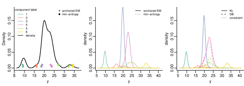
The middle and right panels of Figure 1 display Monte Carlo estimates of the scaled component densities. The scaled component density for $j$ is $\eta_{j}\phi_{p}(\cdot,\gamma_{j})$; as noted by Rodriguez and Walker, (2014), accurate posterior inference on this quantity is tantamount to inference on the posterior classification probability to component $j$. For components 1, 3, 4, and 6, all methods produce unimodal densities that are similar in location The estimated density of component 2 has an irregular shape for all methods: the density is skewed under the anchored models and KL relabeling and it is bimodal under the ordering constraint. The location of component 5 differs between the two anchor models, with the minimum-entropy model placing the component in the right-hand cluster in the data. The relabeling methods estimate a more symmetric density with a mode shifted towards the right.

The posterior means of the component-specific parameters are given in Table 1. The anchored models and relabeling methods produce similar estimates for $\theta_{1}$, $\theta_{3}$, and $\theta_{4}$. For component 4, however, the estimated standard deviations somewhat between the anchor models and relabeling methods, with the estimated values of $\sigma_{4}$ higher under the relabeling methods than the EM anchor model. Both anchor models estimate a greater degree of separation among the means of components 2, 3, 4, and 5 than either of the relabeling methods, which reflects the influence of the separation among the anchor points. Lastly, the parameter estimates for components 5 and 6 under the minimum-entropy model reflect the proximity of the anchor points assigned to these components: both components describe the distinct modal region between 30 and 35, whereas component 5 overlaps with components in the middle region under the other methods. The estimated $\eta$ values are fairly consistent across methods, except for a very low estimate of $\eta_{5}$ under the minimum-entropy model and a tendency for the ordering constraint to produce estimates closer to $1/k$ than the other methods.

Table 1: Posterior means (standard errors) of the component-specific parameters for the galaxies data.

	$\theta_{1}$	$\theta_{2}$	$\theta_{3}$	$\theta_{4}$	$\theta_{5}$	$\theta_{6}$	time(s)
anchored EM	9.713 (0.0022)	16.798 (0.0129)	19.845 (0.0018)	22.803 (0.0038)	25.408 (0.0130)	33.018 (0.0058)	11.91
min-entropy	9.713 (0.0022)	17.289 (0.0214)	19.815 (0.0021)	22.927 (0.0036)	31.512 (0.0181)	33.672 (0.0148)	58.62
KL	9.711 (0.0024)	18.522 (0.0887)	19.847 (0.0169)	22.625 (0.0057)	23.419 (0.0802)	32.795 (0.0223)	183.46
DB	9.711 (0.0024)	18.177 (0.0853)	20.049 (0.0205)	22.222 (0.0130)	23.963 (0.0817)	32.797 (0.0195)	9.04
constraint	8.099 (0.0529)	16.437 (0.0264)	19.878 (0.0118)	22.248 (0.0119)	25.631 (0.0288)	34.625 (0.0553)	N/A
	$\sigma_{1}$	$\sigma_{2}$	$\sigma_{3}$	$\sigma_{4}$	$\sigma_{5}$	$\sigma_{6}$
anchored EM	0.685 (0.0018)	1.104 (0.0058)	0.756 (0.0013)	1.110 (0.0024)	1.289 (0.0050)	1.097 (0.0038)
min-entropy	0.682 (0.0018)	1.253 (0.0083)	0.755 (0.0017)	1.490 (0.0031)	1.214 (0.0076)	1.134 (0.0069)
KL	0.708 (0.0037)	1.131 (0.0048)	0.794 (0.0031)	1.610 (0.0020)	1.315 (0.0045)	1.171 (0.0031)
DB	0.709 (0.0020)	1.080 (0.0055)	0.825 (0.0030)	1.741 (0.0065)	1.197 (0.0048)	1.178 (0.0051)
constraint	0.749 (0.0031)	0.987 (0.0047)	1.078 (0.0058)	1.369 (0.0056)	1.359 (0.0048)	1.185 (0.0056)
	$\eta_{1}$	$\eta_{2}$	$\eta_{3}$	$\eta_{4}$	$\eta_{5}$	$\eta_{6}$
anchored EM	0.090 (0.0002)	0.055 (0.0005)	0.374 (0.0007)	0.330 (0.0009)	0.105 (0.0008)	0.046 (0.0002)
min-entropy	0.091 (0.0002)	0.078 (0.0011)	0.348 (0.0007)	0.415 (0.0011)	0.038 (0.0003)	0.029 (0.0002)
KL	0.090 (0.0002)	0.041 (0.0003)	0.323 (0.0009)	0.404 (0.0011)	0.097 (0.0007)	0.045 (0.0002)
DB	0.090 (0.0002)	0.052 (0.0005)	0.312 (0.0009)	0.376 (0.0013)	0.124 (0.0010)	0.046 (0.0002)
constraint	0.082 (0.0003)	0.103 (0.0010)	0.294 (0.0013)	0.301 (0.0013)	0.178 (0.0014)	0.042 (0.0002)

Table 1 also reports the CPU times for implementing each method using an Intel Core i7-8700 processor. For the anchor models, these times are the pre-processing times required to select anchor points. For the relabeling methods, the reported times are for post-processing of the posterior samples and are thus dependent on the number of posterior samples retained for the analysis. None of the reported times includes the time required to sample from the posterior distributions.

4.3 Simulated data

We next fit anchor models to data generated from three univariate Gaussian mixtures with the parameters given in Table 2.

Table 2: Model parameters used in the simulations.

		Model 1	Model 2	Model 3
	$\eta$	$(0.65,0.35)$	$(0.25,0.25,0.25,0.25)$	$(0.2,0.2,0.25,0.2,0.15)$
	$\theta$	$(0,0)$	$(-3,-1,1,3)$	$(19,19,23,29,33)$
	$\sigma$	$(0.5,1.5)$	$(1,1,1,1)$	$(2.236,1,1,0.707,1.414)$

The density functions of models 1, 2, and 3 are shown in the left panels of Figures 2, 3, and 4, respectively. Model 1 is a scale mixture whose two components have identical locations. Models 2 and 3 have been studied previously by Papastamoulis and Iliopoulos, (2010) (Model 3) and Rodriguez and Walker, (2014) (Models 2 and 3) to assess performance of relabeling algorithms. We drew samples of size $n=200$ from Models 1 and 2 and $n=600$ from Model 3. Following the approach of Rodriguez and Walker, (2014), we used “perfect samples,” evenly-spaced quantiles of the mixture distribution as evaluated using the R package nor1mix (Maechler,, 2019), to eliminate sampling variability.

For each model, we fit three anchor models using the anchored EM method and the minimum-entropy method described in Section 4.2. The third anchor model is an “oracle” model, in which the anchor points are selected to be the observations closest to predetermined quantiles of each true component density. Such information about the true densities would not be available in practice, but we present these results as an illustration of the model’s performance when anchor points represent known features of the true mixture components. For the anchor models, we report the value of $\alpha$ evaluated at the true $\mbox{\boldmath$\gamma$}_{0}$. Finally, we fit the exchangeable model and applied the KL and DB relabeling methods and prior ordering constraints.

The following priors and hyperparameters were specified for each example, adhering to the recommendations of Richardson and Green, (1997): $\theta_{j}$ has a Normal distribution with mean $\mu$ and variance $1/\kappa$, $\sigma_{j}^{-2}$ has a Gamma$(a_{0},b_{0})$ distribution, $j=1,\ldots,k$, and $\eta$ has a Dirichlet$(\mbox{\boldmath$1$}_{k})$ distribution. Letting $R=y_{(n)}-y_{(1)}$, where $y_{(h)}$ denotes the $h$th order statistic, the hyperparameters were set as: $\mu=\bar{y}$, $\kappa=1/R^{2}$, $a_{0}=2$, $b_{0}\sim$Gamma($g_{0}$, $h_{0}$), $g_{0}=0.2$, and $h_{0}=10/R^{2}$.

The following results use $m_{j}=1$, $j=1,\ldots,k$ (one anchor point per component) for the three anchor models. The oracle anchor points are the observations closest to the median of each component. The Appendix presents results from using two anchor points per component.

4.3.1 Model 1.

Figure 2: Left panel: mixture density, anchor points, and true scaled component densities for model 1. Middle panel: estimated scaled component densities for the anchor models. Right panel: estimated scaled component densities for the relabeling methods.

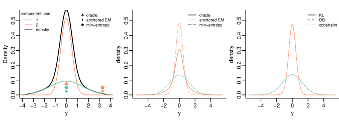
Model 1 is a scale mixture whose two components both have means of zero. The oracle anchors are nearly identical points at the median of the distribution. The anchored EM and minimum-entropy methods select the same anchor points in this example: the maximum observation is anchored to component 1 while the observation closest to the sample mean is anchored to component 2. These two anchor models have $\alpha$ values of 1.000, while the oracle anchor model has an $\alpha$ value of 0.500. Figure 2 shows the anchor points and the estimated scaled component densities, and Table 3 gives the estimated posterior means of the component-specific parameters and the total absolute errors, calculated as $\sum_{j=1}^{k}|a_{j}-\widehat{a}_{j}|$ for a parameter $a_{j}$ having posterior mean equal to $\widehat{a}_{j}$. For this example, the ordering constraint $\sigma_{1}>\sigma_{2}$ was used. The estimates are very similar across the methods for these data, with the exception of the oracle anchor model. The oracle model performs poorly, producing identical parameter estimates for both components, because the anchor points provide no information about the scale difference between the components. None of the methods accurately capture the difference between $\eta_{1}$ from $\eta_{2}$, with the anchored EM and minimum-entropy models coming the closest of the six methods.

Table 3: Posterior means (standard errors) of the component-specific parameters for Model 1.

	$\theta_{1}$	$\theta_{2}$	error	time (s)
true	1.5	0.5	N/A
oracle anchors	0.0010 (0.0010)	-0.0010 (0.0010)	0.0020	N/A
anchored EM	-0.0027 (0.0014)	-0.0009 (0.0005)	0.0036	1.03
min-entropy	-0.0003 (0.0014)	-0.0006 (0.0005)	0.0009	0.50
KL	0.0007 (0.0013)	0.0005 (0.0005)	0.0012	584.25
DB	0.0010 (0.0013)	0.0002 (0.0006)	0.0012	574.00
constraint	0.0011 (0.0013)	0.0001 (0.0006)	0.0012	N/A
	$\sigma_{1}$	$\sigma_{2}$	error
true	0.35	0.65	N/A
oracle anchors	0.867 (0.0035)	0.866 (0.0035)	0.9988
anchored EM	1.320 (0.0013)	0.467 (0.0006)	0.2125
min-entropy	1.320 (0.0013)	0.468 (0.0006)	0.2122
KL	1.309 (0.0013)	0.464 (0.0006)	0.2272
DB	1.309 (0.0013)	0.464 (0.0006)	0.2272
constraint	1.309 (0.0013)	0.464 (0.0006)	0.2272
	$\eta_{1}$	$\eta_{2}$	error
true	0.35	0.65	N/A
oracle anchors	0.501 (0.0009)	0.499 (0.0009)	0.302
anchored EM	0.430 (0.0009)	0.570 (0.0009)	0.1594
min-entropy	0.428 (0.0009)	0.572 (0.0009)	0.1568
KL	0.438 (0.0009)	0.562 (0.0009)	0.1766
DB	0.439 (0.0009)	0.561 (0.0009)	0.1772
constraint	0.439 (0.0009)	0.561 (0.0009)	0.1771

4.3.2 Model 2.

Figure 3: Left panel: mixture density, anchor points, and true scaled component densities for model 2. Middle panel: estimated scaled component densities for the anchor models. Right panel: estimated scaled component densities for the relabeling methods.

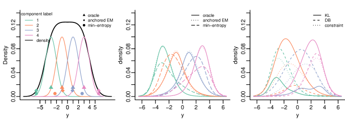
The component densities of Model 2 overlap substantially, with equal variances and evenly-spaced means. The true model and estimated anchor points are shown in the left panel of Figure 3, with $\alpha$ values of 0.947, 0.972, and 0.996 for the oracle, anchored EM, and minimum-entropy models, respectively. The EM and minimum-entropy method both select the minimum and maximum observations to be anchored to components 1 and 4, respectively. For components 2 and 3, the anchored EM points fall near the true component means of -1 and 1, while the minimum-entropy points fall closer to -2 and 2, respectively. The effect of these differences is seen in the middle panel of Figure 3. The estimated scaled densities for components 2 and 3 are approximately symmetric under the EM anchor model. Under the minimum entropy model, however, these densities are skewed, with excess mass near the anchor points, and the posterior means of $\theta_{2}$ and $\theta_{3}$, shown in Table 4, are poor estimates of the true component means. Both of the relabeling methods produce estimated component means that are biased towards zero, most substantially for components 2 and 3, and severely overestimate $\eta_{2}$ while underestimating $\eta_{3}$. The oracle and the EM anchor models produce relatively accurate estimates of all model parameters.

Table 4: Posterior means (standard errors) of the component-specific parameters for Model 2.

	$\theta_{1}$	$\theta_{2}$	$\theta_{3}$	$\theta_{4}$	error	time (s)
true	-3	-1	1	3
oracle anchors	-2.819 (0.0049)	-0.960 (0.0072)	0.956 (0.0072)	2.818 (0.0049)	0.448	N/A
anchored EM	-2.983 (0.0069)	-0.960 (0.0073)	0.997 (0.0073)	2.997 (0.0068)	0.063	24.87
min-entropy	-2.967 (0.0116)	-1.653 (0.0095)	1.965 (0.0088)	2.864 (0.0134)	1.786	10.37
KL	-1.773 (0.0344)	-1.529 (0.0084)	1.194 (0.0339)	2.074 (0.0069)	2.876	7031.77
DB	-2.556 (0.0142)	-0.250 (0.0384)	0.260 (0.0143)	2.513 (0.0196)	2.421	169.71
constraint	-3.483 (0.0231)	-1.038 (0.0121)	1.034 (0.0124)	3.453 (0.0231)	1.008	N/A
	$\sigma_{1}$	$\sigma_{2}$	$\sigma_{3}$	$\sigma_{4}$	error
true	1	1	1	1
oracle anchors	1.024 (0.0026)	1.067 (0.0041)	1.063 (0.0039)	1.026 (0.0025)	0.1805
anchored EM	1.074 (0.0025)	0.984 (0.0031)	0.984 (0.0032)	1.069 (0.0025)	0.1752
min-entropy	1.121 (0.0040)	1.089 (0.0036)	1.042 (0.0034)	1.168 (0.0043)	0.4192
KL	0.749 (0.0067)	1.449 (0.0023)	0.715 (0.0069)	1.304 (0.0031)	1.2890
DB	1.077 (0.0033)	0.698 (0.0028)	1.455 (0.0051)	0.987 (0.0032)	0.8471
constraint	0.984 (0.0038)	1.124 (0.0047)	1.122 (0.0047)	0.988 (0.0038)	0.2733
	$\eta_{1}$	$\eta_{2}$	$\eta_{3}$	$\eta_{4}$	error
true	0.25	0.25	0.25	0.25
oracle anchors	0.247 (0.0011)	0.252 (0.0013)	0.251 (0.0013)	0.250 (0.0010)	0.0059
anchored EM	0.255 (0.0012)	0.247 (0.0012)	0.247 (0.0012)	0.251 (0.0012)	0.0124
min-entropy	0.222 (0.0016)	0.283 (0.0016)	0.263 (0.0014)	0.232 (0.0018)	0.0923
KL	0.100 (0.0007)	0.439 (0.0016)	0.082 (0.0006)	0.379 (0.0015)	0.6357
DB	0.275 (0.0015)	0.078 (0.0007)	0.418 (0.0022)	0.230 (0.0014)	0.3844
constraint	0.224 (0.0017)	0.275 (0.0020)	0.274 (0.0019)	0.226 (0.0017)	0.0992

4.3.3 Model 3

Figure 4: Left panel: mixture density, anchor points, and true scaled component densities for model 3. Middle panel: estimated scaled component densities for the anchor models. Right panel: estimated scaled component densities for the relabeling methods.

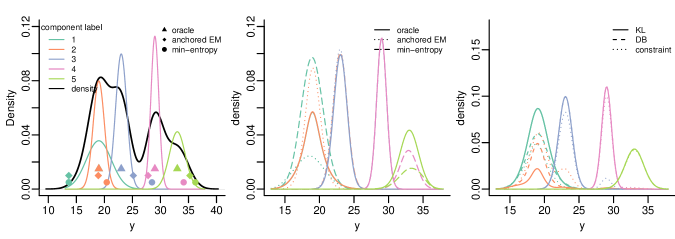
Model 3 is a five-component mixture in which the components have varying locations, scales, and weights, except components 1 and 2, which have identical locations. The true scaled component densities and anchor points are shown in Figure 4 and the posterior parameter estimates are given in Table 5. The$\alpha$ values for the oracle, anchored EM, and minimum-entropy models are 0.500, 1.000, and 0.978, respectively. The anchored EM points are offset from the true component means but still tend to fall in regions to which their component’s true density assigns sizable mass. This model produces accurate estimates of $\theta_{2}-\theta_{5}$, but incorrectly estimates a substantial location shift between components 1 and 2. Its estimates of the component standard deviations are close to their true values, except that of $\sigma_{1}$, which is underestimated as it is by all other methods. The KL and DB relabeling methods accurately estimate the means and standard deviations of all components, and the DB method also produces accurate estimates of $\eta$. Under the ordering constraint, the estimated scaled densities of components 2 and 3 are multimodal and the estimates of $\theta$ are comparatively inaccurate, reflecting the inadequacy of this constraint to describe overlapping components.

Table 5: Posterior means (standard errors) of the component-specific parameters for Model 3.

	$\theta_{1}$	$\theta_{2}$	$\theta_{3}$	$\theta_{4}$	$\theta_{5}$	error	time (s)
true	19	19	23	29	33
oracle anchors	18.955 (0.0049)	18.958 (0.0049)	23.030 (0.0014)	29.006 (0.0006)	32.990 (0.0016)	0.135	N/A
anchored EM	17.273 (0.0290)	19.049 (0.0019)	22.975 (0.0014)	29.006 (0.0006)	32.991 (0.0016)	1.816	16.60
min-entropy	18.948 (0.0014)	23.011 (0.0010)	29.006 (0.0006)	33.031 (0.0056)	33.838 (0.0100)	14.94	10.56
KL	19.080 (0.0028)	20.037 (0.0876)	23.029 (0.0016)	29.006 (0.0007)	32.993 (0.0018)	1.159	1106.45
DB	20.376 (0.0698)	18.732 (0.0417)	23.035 (0.0018)	29.007 (0.0007)	32.995 (0.0018)	1.691	287.54
constraint	17.808 (0.0288)	20.061 (0.0299)	23.847 (0.0360)	29.262 (0.0122)	33.167 (0.0146)	3.529	N/A
	$\sigma_{1}$	$\sigma_{2}$	$\sigma_{3}$	$\sigma_{4}$	$\sigma_{5}$	error
true	2.236	1	1	0.7071	1.414
oracle anchors	1.371 (0.0048)	1.380 (0.0048)	0.973 (0.0010)	0.719 (0.0005)	1.364 (0.0012)	1.334
anchored EM	1.490 (0.0081)	1.073 (0.0042)	1.011 (0.0009)	0.719 (0.0005)	1.363 (0.0012)	0.892
min-entropy	1.606 (0.0010)	1.011 (0.0007)	0.718 (0.0005)	1.067 (0.0025)	1.134 (0.0037)	1.563
KL	1.582 (0.0047)	0.976 (0.0051)	0.974 (0.0011)	0.716 (0.0005)	1.358 (0.0013)	0.769
DB	1.538 (0.0080)	1.020 (0.0053)	0.974 (0.0011)	0.716 (0.0005)	1.358 (0.0013)	0.810
constraint	1.325 (0.0050)	1.265 (0.0061)	0.934 (0.0022)	0.745 (0.0018)	1.337 (0.0019)	1.356
	$\eta_{1}$	$\eta_{2}$	$\eta_{3}$	$\eta_{4}$	$\eta_{5}$	error
true	0.2	0.2	0.25	0.2	0.15
oracle anchors	0.201 (0.0008)	0.204 (0.0008)	0.245 (0.0003)	0.201 (0.0001)	0.149 (0.0001)	0.0127
anchored EM	0.132 (0.0021)	0.255 (0.0019)	0.264 (0.0003)	0.201 (0.0001)	0.149 (0.0001)	0.1387
min-entropy	0.392 (0.0002)	0.255 (0.0002)	0.200 (0.0002)	0.088 (0.0004)	0.064 (0.0004)	0.4954
KL	0.335 (0.0010)	0.073 (0.0008)	0.246 (0.0005)	0.198 (0.0002)	0.147 (0.0002)	0.2691
DB	0.257 (0.0015)	0.151 (0.0018)	0.246 (0.0005)	0.198 (0.0002)	0.147 (0.0002)	0.1146
constraint	0.191 (0.0023)	0.252 (0.0012)	0.228 (0.0010)	0.186 (0.0007)	0.143 (0.0003)	0.1034

The minimum entropy model performs poorly for these data: the anchor points are located at the periphery of plausible regions under their respective component densities, with no points near regions of high density around the mean of component 3. As a result, the mass at this peak is split between components 2 and 3 and the estimated scaled component densities for components 2 and 3 appear bimodal. A similar phenomenon produces bimodality in component 4. Table 5 shows that this model produces the least accurate estimates of all of the methods, especially for the component means.

In each of these univariate examples, the anchored EM algorithm has selected anchor points that result in comparatively accurate estimates of the component-specific parameters. In terms of absolute relative error, it outperforms the minimum-entropy anchor model in all cases and tends to have comparable or superior performance to the relabeling methods. Interestingly, the anchored EM model occasionally performs better than the oracle model, due to the anchor points’ ability to provide information about both the locations and the relative scales of the components. The estimates produced by the minimum entropy model are less accurate because this method tends to select points in low-density areas where adjacent component begin to overlap. Although these points maximize the model’s estimated asymptotic identifiability, their influence introduces bias in finite samples. It is evident that anchor points must fall in areas with non-negligible density of the components to which they belong.

5 A multivariate example: fall detection data

We now apply the anchored modeling framework to a data set called SisFall (Sucerquia et al.,, 2017), one of a growing body of fall data sets that are being used to develop systems that detect falls automatically using wearable devices, cameras, and/or microphones. Experimental data are obtained from volunteer subjects who simulate falls and various activities of daily living (ADLs) and analyzed with the goal of characterizing the distinguishing features of falls compared to ADLs and detecting falls with high accuracy. Common practices in analyzing these types of data include thresholding (Bourke and Lyons,, 2008), in which lower- or upper-thresholds for one variable are set, and a fall is determined to have occurred if the variable exceeds the threshold during a trial. More recent analyses have used supervised classification algorithms on extracted features of the data (Albert et al.,, 2012; Casilari et al.,, 2017). Our approach uses a finite Gaussian mixture model to cluster activities into similar subgroups and to provide a characterization of the features of each group. Analyzing these data in a mixture framework makes it possible to identify groups of experimental activities that share similar features and to describe, with an accompanying appraisal of uncertainty, the typical features of each group. Using this model for classification can provide further insight about which types of ADLs are difficult to distinguish from falls.

The subjects of the SisFall experiments performed $15$ types of falls and $19$ types of ADLs, repeating $5$ trials for most of the activities, while wearing two accelerometers and one gyroscope. We analyzed the data recorded by one of the two accelerometers worn by one subject (“Subject 9”, a 24-year-old male) in the SisFall dataset. A time series of three-dimensional acceleration vectors $(x_{t},y_{t},z_{t})$ is available for each of the $154$ trials. Following common practice in the fall detection literature, we summarized the acceleration at each time point $t$ via the Signal Magnitude Vector (SMV), defined as $SMV_{t}=\sqrt{x_{t}^{2}+y_{t}^{2}+z_{t}^{2}}$. We further summarized the SMV series for each trial using the logarithm of three extracted features arranged in a three-dimensional vector. These features, previously used by Casilari et al., (2017) in analyzing several similar fall data sets, are: $\log\left(\max_{t}SMV_{t}\right)$, $\log\left(\min_{t}SMV_{t}\right)$, and $\log\left(\max_{t}|SMV_{t}-SMV_{t-1}|\right)$. Ultimately, the resulting data set contained $154$ three-dimensional vectors of extracted log-features.

Figure 5: The data and selected anchor points for the SisFall data example.

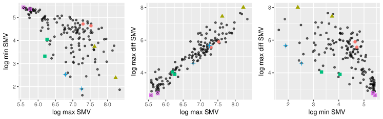
We fit a multivariate Gaussian mixture model with $k=5$ components. We selected the number of components based on the Bayesian information criterion (BIC) evaluated at MAP estimates of the exchangeable model parameters. We specified a $N_{3}(\mbox{\boldmath$\mu$},\mbox{\boldmath$\Sigma$}_{j}/\kappa)$ prior on $\mbox{\boldmath$\theta$}_{j}$ with $\mbox{\boldmath$\mu$}=\bar{\mbox{\boldmath$Y$}}$, the sample mean vector of the data, and $\kappa=0.01$. We specified a Wishart $(\nu,\mbox{\boldmath$A$})$ distribution on $\mbox{\boldmath$\Sigma$}_{j}^{-1}$ with $\nu=6$ degrees of freedom and prior scale $\mbox{\boldmath$A$}=5\mbox{\boldmath$I$}_{3}$, where $\mbox{\boldmath$I$}_{p}$ denotes the $p\times p$ identity matrix. Finally, we specified a Dirichlet$(\mbox{\boldmath$1$}_{3})$ prior for $\eta$. We used the anchored EM algorithm to select two anchor points per component. The data and selected anchor points are shown in Figure 5. The coefficient of quasi-consistency was estimated as $\widehat{\alpha}>0.9999$. Qualitatively, the selected anchor points identify well-separated sites on the periphery of the data cloud, as we would expect in a location problem by generalizing the intuition provided by Proposition 4. The high value of $\widehat{\alpha}$ indicates that we can expect our anchor points to produce high posterior concentration on the true parameter values in large samples. We fit the model using a Gibbs sampler with $200$ parallel chains. We thinned the chains after $5,000$ burn-in iterations to obtain $M=50,000$ samples from the posterior distribution.

Posterior density estimates of $\theta$ are shown in Figure 6. Table A11 lists the average posterior allocation probabilities for selected activities, where each trial’s probability of allocation to component $j$ is the relative frequency that $s_{i}^{m}=j$, calculated from the Monte Carlo posterior samples of $\mbox{\boldmath$s$}^{m}$, $m=1,\ldots,M$. The table gives these probabilities averaged over the repeated trials for each activity. The legend of Figure 6 also displays the proportion of falls among the observations classified to each component, if each trial is classified to its most probable component.

Figure 6: 2D marginal density estimates of the posterior distribution of $\mbox{\boldmath$\theta$}_{j}$ for the fall dataset.

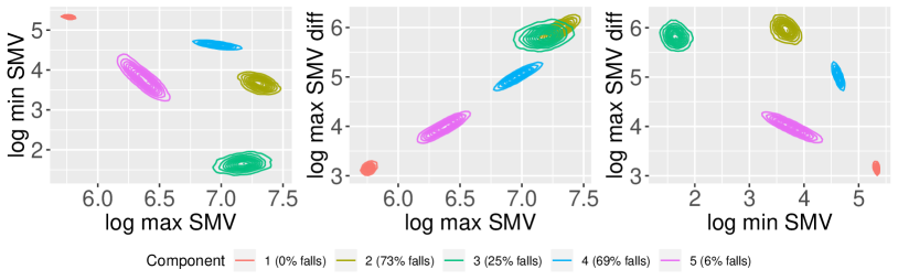
Component 1, whose mean is located in a far corner of the posterior parameter space, is characterized by low values of maximum SMV and high values of minimum SMV throughout the trial. It is unsurprising that no activities classified to this component are falls because falls are expected to be associated with large changes in acceleration. Component 5 describes activities with slightly higher values of maximum difference in SMV, and, unlike component 1, is estimated to contain a small number of falls. Table A11 indicates that quick vertical movements, such as quickly sitting and standing (D10), are likely to be classified to this component.

Components 2 and 4 both exhibit high values of maximum SMV and maximum difference in SMV. The majority of activities classified to these components are falls, with a few ADLs such as moving up and down stairs (D06), or trying to get up but collapsing into a chair (D11). The forward falls tend to be classified into component 2, whose SMV values are higher, while falls in other directions are classified into component 4. Component 3, like component 2, describes activities with very high values of maximum SMV and maximum difference, but unlike component 2 its average value of minimum SMV is low. This component contains only 25% falls, suggesting that minimum SMV is a feature that is able to distinguish ADLs from falls.

Table 6: Posterior allocation probabilities for selected activities in the SisFall dataset.

Activity	Component
	1	2	3	4	5
D03 Jogging slowly	0.000	0.000	1.000	0.000	0.000
D06 Walking upstairs and downstairs quickly	0.000	0.796	0.188	0.000	0.016
D07 Slowly sit in a half height chair, wait a moment, and up slowly	0.981	0.000	0.000	0.006	0.013
D09 Slowly sit in a low height chair, wait a moment, and up slowly	0.245	0.050	0.000	0.575	0.131
D10 Quickly sit in a low height chair, wait a moment, and up quickly	0.001	0.042	0.001	0.148	0.808
D11 Sitting a moment, trying to get up, and collapse into a chair	0.000	0.541	0.003	0.454	0.002
D18 Stumble while walking	0.000	0.957	0.003	0.040	0.000
D19 Gently jump without falling (trying to reach a high object)	0.000	0.308	0.033	0.000	0.658
F02 Fall backward while walking caused by a slip	0.000	0.302	0.001	0.697	0.000
F04 Fall forward while walking caused by a trip	0.000	0.938	0.001	0.061	0.000
F09 Lateral fall when trying to get up	0.000	0.074	0.000	0.926	0.000
F10 Fall forward when trying to sit down	0.000	0.609	0.001	0.390	0.000

Table A11 indicates that certain types of ADLs, such as sitting slowly (D07), are unlikely to be confused with falls as indicated by their high probability of allocation to component 1. The small maximum change in (log) acceleration associated with this component, is a feature that is likely to be highly predictive of certain ADLs. Other ADLs, such as going upstairs quickly (D06), share the high-acceleration features that many falls exhibit. The similarities between ADLs that involve fast movement and forward falls suggest that additional measurements, perhaps some including a directional component, may aid in better distinguishing falls in these difficult cases.

6 Discussion

The proposed anchored Bayesian mixture model offers a model-based resolution to label-switching that eliminates prior and posterior exchangeability without imposing highly restrictive identifiability constraints. In Section 2.5 we introduced a notion of quasi-consistency which guarantees that, in large samples, a well-specified anchor model places high posterior probability on one relabeling of the true component-specific parameters. Our anchored EM strategy for selecting optimal anchor points requires several pre-processing steps, but eliminates the need for post-processing of MCMC samples, often resulting in computational savings. A carefully-specified anchor model will produce component-specific parameter estimates that reflect homogeneous subgroups in the population and arise directly from the specified model.

The examples presented in this paper have demonstrated that one or two anchor points per component are often sufficient to eliminate posterior multimodality and produce accurate parameter estimates. The optimal number of anchor points may, in some situations, be higher, and may depend on the method used to select the points. Future work will investigate this question in a variety of univariate and multivariate settings.

Non-Gaussian components.

The anchor model methodology is readily applicable to non-Gaussian component distributions. The model properties that we presented in this paper do not, in general, rely on Gaussian components. Anchoring always eliminates the model’s posterior exchangeability and a minimal number of anchor points will typically produce distinct distributions for the $\gamma_{j}$, as outlined in Proposition 2, when the component distributions are continuous in $y$ and $\gamma$. Proposition 5, which stated that the anchor model’s fit improves with the addition of more anchor points, is also true for non-Gaussian mixtures under fairly general conditions. The asymptotic result in Section 2.5 does depend on several regularity conditions on the component likelihoods and priors, which may not hold for all choices of component distributions. The anchored EM algorithm of Section 3 can be implemented in models from other families. Our own applied work (Kunkel and Peruggia,, 2019) has demonstrated the use of this strategy in a Gaussian mixture of regressions model. Different component distributions will motivate new approaches to specifying anchor points and these are interesting directions of future research.

Other extensions.

Future work will explore ways to quantify the sensitivity of analyses to changes in the specification of the anchor points and the number of anchor points. An interesting feature of anchor models is that they admit the possibility of using improper priors for the component-specific parameters. Sensitivity to proper priors is a well-known issue in mixture modeling (Richardson and Green,, 1997; Frühwirth-Schnatter,, 2006) but non-informative priors are difficult to derive because improper priors typically lead to improper posteriors (Grazian and Robert,, 2018). An anchor model can restrict the space of latent allocations to prevent empty components, similarly to the methods proposed by Diebolt and Robert, (1994) and Wasserman, (2000), and this possibility allows investigation of the model’s behavior under a wider class of priors.

From an applied modeling perspective, we plan to extend the anchored mixture methodology to the case of hierarchical mixture models fit to grouped data collected on many experimental units, as in the case, for example, of the entire SisFall data set. Assuming a mixture model with a fixed number of components for the data collected on each of the experimental units, with component specific parameters tied together in a hierarchical structure, several challenging modeling questions will need an answer. Decisions will have to be made concerning the number of components needed to describe the data for each experimental unit. A simple approach would employ the same number (possibly random) of components for each subject. A more refined approach would allow for varying numbers of components across units. With specific regard to the anchored methodology, we plan to investigate different approaches to the specification of the anchor points. These include selecting anchor points using independent fits to the data for each unit and strategies that account for existing dependencies in the data. We will also consider approaches where only a subset of the units will have anchored observations.

Anchored Bayesian Gaussian Mixture Models

Deborah Kunkel and Mario Peruggia

Appendix

Appendix A Proofs of the propositions

This section presents proofs of Propositions 1 and 3-6. When necessary, references to expressions in the main manuscript will be preceded by M, so that, for example, (M2) refers to Equation (2) in the main manuscript.

Proposition 1

The following two statements hold under conditions C.1 and C.2.

1. An anchor model $A=\{A_{1},\ldots,A_{k}\}$ imposes a unique labeling on each partition that has nonzero probability if and only if $A_{1},\ldots,A_{k-1}$ are non-empty; that is, $k_{0}\geq k-1$.

2. For any $j\leq k_{0}$, $j\neq j\prime$, the marginal posterior density of $\mbox{\boldmath$\gamma$}_{j}$ is distinct from the marginal posterior density of $\mbox{\boldmath$\gamma$}_{j\prime}$ with probability 1.

Proof of part a.

Suppose $A_{k-1}$ and $A_{k}$ are empty so that at least two components have no points anchored to them. Choose an allocation $\mbox{\boldmath$s$}^{*}$ from $\mathscr{S}^{A}$ such that $\mbox{\boldmath$s$}^{*}$ has at least one element equal to $k-1$, so that $\mbox{\boldmath$s$}^{*}$ has induced a partition of the data under which one group is labeled $k-1$. The set $\mathscr{S}^{A}$ also contains the allocation obtained by permuting the label $k$ and $k-1$ in $\mbox{\boldmath$s$}^{*}$, which induces the same partition but a different labeling. In contrast, if $A_{1},\ldots,A_{k-1}$ each contain at least one point, any allocation from $\mathscr{S}^{A}$ induces a partition that cannot be relabeled without relabeling an anchor point.

Proof of part b.

Assume that component $j$ has at least one anchor point; that is, $A_{j}\neq\emptyset$, and that $\mbox{\boldmath$x$}_{h}$ denotes the anchor points for component $h$. Use $\mbox{\boldmath$\gamma$}_{-(h)}$ to denote $\mbox{\boldmath$\gamma$}=(\mbox{\boldmath$\gamma$}_{1},\ldots,\mbox{\boldmath$\gamma$}_{h-1},\mbox{\boldmath$\gamma$}_{h+1},\ldots,\mbox{\boldmath$\gamma$}_{k})$ and $\Gamma$ to denote the parameter space of $\mbox{\boldmath$\gamma$}_{h}$. The posterior density of $\mbox{\boldmath$\gamma$}_{j}$, denoted by $p_{j}(\mbox{\boldmath$\gamma$}_{j}|\mbox{\boldmath$y$})$, satisfies

$$p_{j}(\mbox{\boldmath$\gamma$}_{j}|\mbox{\boldmath$y$})\propto \int_{\mbox{\boldmath$\gamma$}_{-(j)}}\int_{\mbox{\boldmath$\eta$}}p(\mbox{\boldmath$\gamma$}_{1},\ldots,\mbox{\boldmath$\gamma$}_{k},\mbox{\boldmath$\eta$},\mbox{\boldmath$y$})d\mbox{\boldmath$\eta$}d\mbox{\boldmath$\gamma_{-(j)}$}$$ (17)

$$= \int_{\mbox{\boldmath$\gamma$}_{-(j)}}\int_{\mbox{\boldmath$\eta$}}\pi(\mbox{\boldmath$\eta$})\prod_{h=1}^{k_{0}}\phi_{p}(\mbox{\boldmath$x$}_{h};\mbox{\boldmath$\gamma$}_{h})\prod_{h=1}^{k}\pi(\mbox{\boldmath$\gamma$}_{h})\prod_{i\not\in A}\sum_{h=1}^{k}\eta_{h}\phi_{p}(y_{i};\mbox{\boldmath$\gamma$}_{h})d\mbox{\boldmath$\eta$}d\mbox{\boldmath$\gamma$}_{-(j)}.$$ (18)

Case 1: $A_{j\prime}\neq\emptyset$.

Define $c(\mbox{\boldmath$\gamma$}_{j},\mbox{\boldmath$\gamma$}_{j\prime})$ to be equal to the following function:

$$c(\mbox{\boldmath$\gamma$}_{j},\mbox{\boldmath$\gamma$}_{j\prime}) =\int_{\mbox{\boldmath$\gamma$}_{-(j,j\prime)}}\prod_{h\neq j,j\prime}^{k_{0}}\phi_{p}(\mbox{\boldmath$x$}_{h};\mbox{\boldmath$\gamma$}_{h})\prod_{h\neq j,j\prime}^{k}\pi(\mbox{\boldmath$\gamma$}_{h})\int_{\mbox{\boldmath$\eta$}}\pi(\mbox{\boldmath$\eta$})\prod_{i\not\in A}\sum_{h=1}^{k}\eta_{h}\phi_{p}(y_{i};\mbox{\boldmath$\gamma$}_{h})d\mbox{\boldmath$\eta$}d\mbox{\boldmath$\gamma$}_{-(j,j\prime)},$$ (19)

noting that the label-invariance of the mixture likelihood gives

$$c(\mbox{\boldmath$u$},\mbox{\boldmath$w$})=c(\mbox{\boldmath$w$},\mbox{\boldmath$u$}).$$ (20)

The expression (18) can be written as

$$p_{j}(\mbox{\boldmath$\gamma$}_{j}|\mbox{\boldmath$y$})\propto \pi(\mbox{\boldmath$\gamma$}_{j})\phi_{p}(\mbox{\boldmath$x$}_{j};\mbox{\boldmath$\gamma$}_{j})\int_{\mbox{\boldmath$w$}}\pi(\mbox{\boldmath$w$})\phi_{p}(\mbox{\boldmath$x$}_{j\prime};\mbox{\boldmath$w$})c(\mbox{\boldmath$w$},\mbox{\boldmath$\gamma$}_{j})d\mbox{\boldmath$w$}.$$ (21)

Further, define

$$c_{2}(\mbox{\boldmath$\gamma$}_{j},\mbox{\boldmath$x$}_{j\prime}) =\int_{\mbox{\boldmath$u$}}\pi(\mbox{\boldmath$u$})\phi_{p}(\mbox{\boldmath$x$}_{j\prime};\mbox{\boldmath$u$})c(\mbox{\boldmath$\gamma$}_{j},\mbox{\boldmath$u$})d\mbox{\boldmath$u$},$$ (22)

yielding

$$p_{j}(\mbox{\boldmath$\gamma$}_{j}|\mbox{\boldmath$y$})\propto \pi(\mbox{\boldmath$\gamma$}_{j})\phi_{p}(\mbox{\boldmath$x$}_{j};\mbox{\boldmath$\gamma$}_{j})c_{2}(\mbox{\boldmath$\gamma$}_{j},\mbox{\boldmath$x$}_{j\prime}).$$ (23)

For component $j\prime$, we have

$$p_{j\prime}(\mbox{\boldmath$\gamma$}_{j\prime}|\mbox{\boldmath$y$})\propto \pi(\mbox{\boldmath$\gamma$}_{j\prime})\phi_{p}(\mbox{\boldmath$x$}_{j\prime};\mbox{\boldmath$\gamma$}_{j\prime})\int_{\mbox{\boldmath$w$}}\pi(\mbox{\boldmath$w$})\phi_{p}(\mbox{\boldmath$x$}_{j};\mbox{\boldmath$w$})c(\mbox{\boldmath$w$},\mbox{\boldmath$\gamma$}_{j\prime})d\mbox{\boldmath$w$}$$ (24)

$$=\pi(\mbox{\boldmath$\gamma$}_{j\prime})\phi_{p}(\mbox{\boldmath$x$}_{j\prime};\mbox{\boldmath$\gamma$}_{j\prime})c_{2}(\mbox{\boldmath$\gamma$}_{j\prime},\mbox{\boldmath$x$}_{j}),$$ (25)

where the second equality follows from (20). Assumption C.2 ensures that there is some open set $W\subset\Gamma$ such that $\pi(\mbox{\boldmath$w$})>0$ for all $\mbox{\boldmath$w$}\in W$. Then for $\mbox{\boldmath$w$}\in W$, we have the posterior density of $\gamma_{j}$ satisfying

$$p_{j}(\mbox{\boldmath$w$}|\mbox{\boldmath$y$})\propto \pi(\mbox{\boldmath$w$})\phi_{p}(\mbox{\boldmath$x$}_{j};\mbox{\boldmath$w$})c_{2}(\mbox{\boldmath$w$},\mbox{\boldmath$x$}_{j\prime}),$$ (26)

while the posterior density of $\mbox{\boldmath$\gamma$}_{j\prime}$ satisfies

$$p_{j\prime}(\mbox{\boldmath$w$}|\mbox{\boldmath$y$})\propto \pi(\mbox{\boldmath$w$})\phi_{p}(\mbox{\boldmath$x$}_{j\prime};\mbox{\boldmath$w$})c_{2}(\mbox{\boldmath$w$},\mbox{\boldmath$x$}_{j}).$$ (27)

With probability 1, $\mbox{\boldmath$x$}_{j}\neq\mbox{\boldmath$x$}_{j\prime}$, and so $p_{j}(\mbox{\boldmath$w$}|\mbox{\boldmath$y$})\neq p_{j\prime}(\mbox{\boldmath$w$}|\mbox{\boldmath$y$})$ for all $\mbox{\boldmath$w$}\in W$.

Case 2.

If $A_{j\prime}=\emptyset$, then

$$p_{j}(\mbox{\boldmath$\gamma$}_{j}|\mbox{\boldmath$y$})\propto \pi(\mbox{\boldmath$\gamma$}_{j})\phi_{p}(\mbox{\boldmath$x$}_{j};\mbox{\boldmath$\gamma$}_{j})\int_{\mbox{\boldmath$w$}}\pi(\mbox{\boldmath$w$})c(\mbox{\boldmath$w$},\mbox{\boldmath$\gamma$}_{j})d\mbox{\boldmath$w$}$$ (28)

while

$$p_{j\prime}(\mbox{\boldmath$\gamma$}_{j\prime}|\mbox{\boldmath$y$})\propto \pi(\mbox{\boldmath$\gamma$}_{j\prime})c_{2}(\mbox{\boldmath$\gamma$}_{j\prime},\mbox{\boldmath$x$}_{j}).$$ (29)

For $\mbox{\boldmath$w$}\in W$, is it clear that $p_{j}(\mbox{\boldmath$w$}|\mbox{\boldmath$y$})\neq p_{j\prime}(\mbox{\boldmath$w$}|\mbox{\boldmath$y$})$.

Proposition 3

The $q$th element of $P_{\mbox{\boldmath$x$}}(\mbox{\boldmath$\gamma$}_{0})$, $p_{q}$, is equal to

$$\prod_{j=1}^{k_{0}}\phi_{p}\left(\mbox{\boldmath$x$}_{j};\mbox{\boldmath$\gamma$}_{0\rho_{q}(j)}\right)\left/\sum_{h=1}^{k!}\prod_{j=1}^{k_{0}}\phi_{p}\left(\mbox{\boldmath$x$}_{j};\mbox{\boldmath$\gamma$}_{0\rho_{h}(j)}\right)\right..$$ (30)

Proof:

The data dependent prior of $(\mbox{\boldmath$\gamma$},\mbox{\boldmath$\eta$})$ under model $A$ is proportional to

$$\pi(\mbox{\boldmath$\eta$})\prod_{j=1}^{k_{0}}p(\mbox{\boldmath$\gamma$}_{j}|\mbox{\boldmath$x$}_{j})\prod_{j=k_{0}+1}^{k}\pi(\mbox{\boldmath$\gamma$}_{j}).$$

The probability of the $q$th class label under the anchor model is

$$p_{q} =\frac{\pi(\rho_{q}(\mbox{\boldmath$\eta$}_{0}))\prod_{j=1}^{k_{0}}p(\mbox{\boldmath$\gamma$}_{0\rho_{q}(j)}|\mbox{\boldmath$x$}_{\rho_{q}(j)})\prod_{j=k_{0}+1}^{k}\pi(\mbox{\boldmath$\gamma$}_{0\rho_{q}(j)})}{\sum_{h=1}^{k!}\pi(\rho_{h}(\mbox{\boldmath$\eta$}_{0}))\prod_{j=1}^{k_{0}}p(\mbox{\boldmath$\gamma$}_{0\rho_{h}(j)}|\mbox{\boldmath$x$}_{j})\prod_{j=k_{0}+1}^{k}\pi(\mbox{\boldmath$\gamma$}_{0\rho_{h}(j)})}$$ (31)

$$=\frac{\prod_{j=1}^{k_{0}}p(\mbox{\boldmath$\gamma$}_{0j}|\mbox{\boldmath$x$}_{j})\prod_{j=k_{0}+1}^{k}\pi(\mbox{\boldmath$\gamma$}_{0\rho_{q}(j)})}{\sum_{h=1}^{k!}\prod_{j=1}^{k_{0}}p(\mbox{\boldmath$\gamma$}_{0\rho_{h}(j)}|\mbox{\boldmath$x$}_{j})\prod_{j=k_{0}+1}^{k}\pi(\mbox{\boldmath$\gamma$}_{0\rho_{h}(j)})},$$ (32)

where the terms $\pi(\rho_{q}(\mbox{\boldmath$\eta$}_{0}))$ are invariant to label permutation and are factored out in (32). For any $q$, we have

$$\prod_{j=1}^{k_{0}}p(\mbox{\boldmath$\gamma$}_{0\rho_{q}(j)})|\mbox{\boldmath$x$}_{j}) =\prod_{j=1}^{k_{0}}\pi(\mbox{\boldmath$\gamma$}_{0\rho_{q}(j)}))\phi_{p}(\mbox{\boldmath$x$}_{j};\mbox{\boldmath$\gamma$}_{0\rho_{q}(j)}))C_{j}^{-1}.$$ (33)

As in Section 2.4 of the manuscript, $C_{j}$ is defined to be

$$C_{j}=\int\pi(\mbox{\boldmath$w$})\phi_{p}(\mbox{\boldmath$x$}_{j};\mbox{\boldmath$w$})d\mbox{\boldmath$w$}$$

and does not depend on the permutation of the label of $\mbox{\boldmath$\gamma$}_{j}$. Further, $\prod_{j=1}^{k}\pi(\mbox{\boldmath$\gamma$}_{\rho_{q}(j)})$ is equal to $\prod_{j=1}^{k}\pi(\mbox{\boldmath$\gamma$}_{\rho_{q\prime}(j)})$ for any $q$ and $q\prime$. The only term in (32) that depends on the $q$th permutation is $\prod_{j=1}^{k_{0}}\phi_{p}(\mbox{\boldmath$x$}_{j};\mbox{\boldmath$\gamma$}_{\rho_{q}(j)})$. Thus the $q$th element of $P_{\mbox{\boldmath$x$}}(\mbox{\boldmath$\gamma$}_{0})$ is equal to

$$p_{q} =\frac{\prod_{j=1}^{k_{0}}\phi_{p}(\mbox{\boldmath$x$}_{j};\mbox{\boldmath$\gamma$}_{0\rho_{q}(j)})}{\sum_{h=1}^{k!}\prod_{j=1}^{k_{0}}\phi_{p}(\mbox{\boldmath$x$}_{j};\mbox{\boldmath$\gamma$}_{0\rho_{h}(j)})}$$

for $q=1,\ldots,k!$.

Proposition 4

Suppose that $p=1$, $k=2$, and that $m_{j}=m$ observations (with $1\leq m\leq n/2$) are to be anchored to component $j$, $j=1,2$. The following results hold:

1. If $\sigma_{1}^{2}=\sigma_{2}^{2}=\sigma^{2}$ and $\theta_{1}<\theta_{2}$, then the optimal anchoring sets $\mbox{\boldmath$x$}_{1}=(y_{(1)},\ldots,y_{(m)})$, $\mbox{\boldmath$x$}_{2}=(y_{(n-m+1)},y_{(n)})$, where $y_{(l)}$ denotes the $l$th order statistic.

2. If $\theta_{1}=\theta_{2}=\theta$ and $\sigma_{1}^{2}<\sigma_{2}^{2}$, then the optimal anchoring sets $\mbox{\boldmath$x$}_{1}$ equal to the points that minimize $\sum_{i=1}^{m}(y_{i}-\theta)^{2}$ and $\mbox{\boldmath$x$}_{2}$ equal to the points that maximize $\sum_{i=1}^{m}(y_{i}-\theta)^{2}$.

Proof.

When $k=2$, $P_{\mbox{\boldmath$x$}}$ has only two elements and maximizing $p_{1}$ will minimize its entropy. Thus, it is sufficient to maximize the ratio $p_{1}/p_{2}$. In the location problem (case 1), $p_{1}/p_{2}$ equals

$$\frac{\phi(\mbox{\boldmath$x$}_{1};\theta_{1},\sigma^{2})\phi(\mbox{\boldmath$x$}_{2};\theta_{2},\sigma^{2})}{\phi(\mbox{\boldmath$x$}_{1};\theta_{2},\sigma^{2})\phi(\mbox{\boldmath$x$}_{2};\theta_{1},\sigma^{2})} =\exp\left(\frac{m}{\sigma^{2}}(\theta_{2}-\theta_{1})(\bar{x}_{2}-\bar{x}_{1})\right),$$

where $\bar{x}_{1}$ and $\bar{x}_{2}$ are the sample means of $\mbox{\boldmath$x$}_{1}$ and $\mbox{\boldmath$x$}_{2}$. Because we assume $\theta_{1}<\theta_{2}$, this expression is increasing in $(\bar{x}_{2}-\bar{x}_{1})$. In case 2, $p_{1}/p_{2}$ is equal to

$$\begin{split}\frac{\phi(\mbox{\boldmath$x$}_{1};\theta,\sigma_{1}^{2})\phi(\mbox{\boldmath$x$}_{2};\theta,\sigma_{2}^{2})}{\phi(\mbox{\boldmath$x$}_{1};\theta,\sigma_{2}^{2})\phi(\mbox{\boldmath$x$}_{2};\theta,\sigma_{1}^{2})}&=\exp\left(\left(\frac{1}{2\sigma_{1}^{2}}-\frac{1}{2\sigma_{2}^{2}}\right)\left(\sum_{i=1}^{m}(x_{2i}-\theta)^{2}-\sum_{i=1}^{m}(x_{1i}-\theta)^{2}\right)\right).\end{split}$$

Because $\sigma_{1}^{2}<\sigma_{2}^{2}$, the ratio is increasing in $\sum_{i=1}^{m}(x_{2i}-\theta)^{2}$ and decreasing in $\sum_{i=1}^{m}(x_{1i}-\theta)^{2}$. This concludes the proof.

Proposition 5

Assume that $\eta_{j}=1/k$, $j=1,\ldots,k$. Let $A_{*}^{1},\ldots,A_{*}^{n}$ be a sequence of anchor models where $A_{*}^{m}$ has the highest marginal likelihood among all anchor models with $m$ anchor points. The marginal likelihoods of the models satisfy $m_{A_{*}^{1}}(\mbox{\boldmath$y$})\leq\ldots\leq m_{A_{*}^{n}}(\mbox{\boldmath$y$})$.

The proof of Proposition 5 below relies on the result stated in the following lemma.

Lemma 1

For any anchor model $A^{m}$, $m\geq 1$, it is possible to form a sequence of anchor models $A^{m},\ldots,A^{n}$ satisfying $A^{m}\subset A^{m+1}\subset\ldots A^{n}$ such that $m_{A^{m}}(\mbox{\boldmath$y$})\leq\ldots\leq m_{A^{n}}(\mbox{\boldmath$y$})$.

Proof.

Given an anchor model $A^{m}$ with $m$ anchor points and some $i\notin A^{m}$, let $A^{m+1}_{i,j}$ denote the anchor model obtained from $A^{m}$ by adding the additional anchor point with index $i$ to component $j$. We will show that for some $j$, the marginal likelihood for $A^{m+1}_{i,j}$ is greater than or equal to that of $A^{m}$.

Let $\mathscr{S}^{A^{m}}$ denote the restricted set of allocation vectors for the anchor model $A^{m}$. It is possible to write $\mathscr{S}^{A^{m}}$ as $\cup_{j=1}^{k}\mathscr{S}^{A^{m+1}_{i,j}}$ for any $i$. The marginal likelihood for $A^{m}$ can be written as

$$m_{A^{m}}(\mbox{\boldmath$y$}) =\sum_{\mathscr{S}^{A^{m}}}m(\mbox{\boldmath$y$}|\mbox{\boldmath$s$})p_{A^{m}}(\mbox{\boldmath$s$})$$

$$=\frac{1}{k^{n-m}}\sum_{\mathscr{S}^{A^{m}}}m(\mbox{\boldmath$y$}|\mbox{\boldmath$s$})$$ (34)

$$=\frac{1}{k}\sum_{j=1}^{k}\frac{1}{k^{n-m-1}}\sum_{\mathscr{S}^{A^{m+1}_{i,j}}}m(\mbox{\boldmath$y$}|\mbox{\boldmath$s$}).$$ (35)

Expression (34) follows from the fact that $p_{A^{m}}(\mbox{\boldmath$s$})=k^{-(n-m)}$ for all $\mbox{\boldmath$s$}\in\mathscr{S}^{A^{m}}$ under the assumption that $\eta_{j}=k^{-1}$, $j=1,\ldots,k$. Expression (35) shows that the marginal likelihood for $A^{m}$ is the average of the marginal likelihoods for $A^{m+1}_{i,j}$, $j=1,\ldots,k$. Thus,

$$m_{A^{m}}(\mbox{\boldmath$y$}) =\frac{1}{k}\sum_{j=1}^{k}\frac{1}{k^{n-m-1}}\sum_{\mathscr{S}^{A^{m+1}_{i,j}}}m(\mbox{\boldmath$y$}|\mbox{\boldmath$s$})$$

$$\leq\max_{j}\frac{1}{k^{n-m-1}}\sum_{\mathscr{S}^{A^{m+1}_{i,j}}}m(\mbox{\boldmath$y$}|\mbox{\boldmath$s$})$$

$$=m_{A^{m}_{i,j^{*}}}(\mbox{\boldmath$y$}),$$ (36)

where $j^{*}$ is the component to which observation $i$ can be anchored to maximize the marginal likelihood. Thus $m_{A^{m}}(\mbox{\boldmath$y$})\leq m_{A^{m+1}_{i,j^{*}}}(\mbox{\boldmath$y$})$ for any $m<n$, proving Lemma 1.

Proposition 5

Assume that $\eta_{j}=1/k$, $j=1,\ldots,k$. Let $A_{*}^{1},\ldots,A_{*}^{n}$ be a sequence of anchor models where $A_{*}^{m}$ has the highest marginal likelihood among all anchor models with $m$ anchor points. The marginal likelihoods of the models satisfy $m_{A_{*}^{1}}(\mbox{\boldmath$y$})\leq\ldots\leq m_{A_{*}^{n}}(\mbox{\boldmath$y$})$.

Proof.

Fix $m$ and let $i$ be the index of an observation not anchored in $A_{*}^{m}$. Then,

$$m_{A_{*}^{m}}(\mbox{\boldmath$y$})\leq m_{A_{i,j^{*}}^{m+1}}(\mbox{\boldmath$y$})\leq m_{A_{*}^{m+1}}(\mbox{\boldmath$y$}),$$

where the first inequality follows from Lemma 1 and the second from the definition of $A_{*}^{m+1}$.

Proposition 6

Let $q$ be the posterior distribution of the allocations under an anchor model, subject to the restrictions in (M15). The KL divergence of $q_{*}$ from $q$, evaluated at a fixed value of $\gamma$, is minimized when the sets $A_{j}$ are chosen to maximize $\sum_{j=1}^{k_{0}}\sum_{i\in A_{j}}r_{ij}$ and when $\widetilde{r}_{ij}=r_{ij}$ for all $i\not\in A$.

Proof.

For any distributions $q$ and $q_{*}$, and defining $x\log(x)=0$, the KL-divergence of $q_{*}$ from $q$ is equal to

$$D_{KL}(q||q_{*}) =\sum_{\mbox{\boldmath$s$}}q(\mbox{\boldmath$s$})\log\left(\frac{q(\mbox{\boldmath$s$})}{q_{*}(\mbox{\boldmath$s$})}\right)$$

$$=\sum_{\mbox{\boldmath$s$}}\left[\prod_{l=1}^{n}q(s_{l})\right]\log\left(\frac{\prod_{i=1}^{n}q(s_{i})}{\prod_{i=1}^{n}q_{*}(s_{i})}\right)$$

$$=\sum_{\mbox{\boldmath$s$}}\left[\prod_{l=1}^{n}q(s_{l})\right]\sum_{i=1}^{n}\left(\log\left(\frac{q(s_{i})}{q_{*}(s_{i})}\right)\right)$$

$$=\sum_{s_{1}=1}^{k}\ldots\sum_{s_{n}=1}^{k}\left[\prod_{l=1}^{n}q(s_{l})\right]\sum_{i=1}^{n}\left(\log\left(\frac{q(s_{i})}{q_{*}(s_{i})}\right)\right)$$

$$=\sum_{s_{1}=1}^{k}\ldots\sum_{s_{n-1}=1}^{k}\left[\prod_{l=1}^{n-1}q(s_{l})\right]\sum_{s_{n}=1}^{k}q(s_{n})\sum_{i=1}^{n}\left(\log\left(\frac{q(s_{i})}{q_{*}(s_{i})}\right)\right)$$

$$\begin{split}&=\sum_{s_{1}=1}^{k}\ldots\sum_{s_{n-1}=1}^{k}\left[\prod_{l=1}^{n-1}q(s_{l})\right]\\ &\;\;\;\;\;\;\;\;\;\;\left[\sum_{s_{n}=1}^{k}q(s_{n})\sum_{i=1}^{n-1}\left(\log\left(\frac{q(s_{i})}{q_{*}(s_{i})}\right)\right)+\sum_{s_{n}=1}^{k}q(s_{n})\left(\log\left(\frac{q(s_{n})}{q_{*}(s_{n})}\right)\right)\right]\end{split}$$

$$=\sum_{s_{1}=1}^{k}\ldots\sum_{s_{n-1}=1}^{k}\left[\prod_{l=1}^{n-1}q(s_{l})\right]\left[\sum_{i=1}^{n-1}\left(\log\left(\frac{q(s_{i})}{q_{*}(s_{i})}\right)\right)+\sum_{s_{n}=1}^{k}q(s_{n})\left(\log\left(\frac{q(s_{n})}{q_{*}(s_{n})}\right)\right)\right]$$

$$\vdots$$

$$=\sum_{i=1}^{n}\sum_{s_{i}=1}^{k}q(s_{i})\log\left(\frac{q(s_{i})}{q_{*}(s_{i})}\right).$$

Substituting the definition of $q_{*}$ in (M13) and the restrictions on $q$ from (M15) yields

$$D_{KL}(q||q_{*}) =\sum_{i=1}^{n}\sum_{j=1}^{k}q(s_{i}=j)\log\left(\frac{q(s_{i}=j)}{r_{ij}}\right)$$

$$=\sum_{i\in A_{j}}\sum_{j=1}^{k}I(s_{i}=j)\log\left(\frac{I(s_{i}=j)}{r_{ij}}\right)+\sum_{i\notin A}\sum_{j=1}^{k}\widetilde{r}_{ij}\log\left(\frac{\widetilde{r}_{ij}}{r_{ij}}\right)$$

$$=-\sum_{j=1}^{k}\sum_{i\in A_{j}}\log\left(r_{ij}\right)+\sum_{j=1}^{k}\sum_{i\notin A}\widetilde{r}_{ij}\log\left(\frac{\widetilde{r}_{ij}}{r_{ij}}\right).$$ (37)

The second term in (37) is non-negative and can be made equal to zero by setting $\widetilde{r}_{ij}=r_{ij}$ for $i\notin A$. The first term decreases toward zero as $r_{ij}\rightarrow 1$ for $i\in A$. Subject to the restriction that $A_{j}\cap A_{j^{\prime}}=\emptyset$ and $|A_{j}|=m_{j}$, the $q$ that minimizes $D_{KL}(q||q_{*})$ is

$$q(S_{i}=j) =\begin{cases}r_{ij}\quad&i\notin A\\ 1\quad&i\in A_{j}\\ 0\quad&i\in A_{j^{\prime}},\quad j^{\prime}\neq j,\end{cases}$$

where the $A_{j}$ are selected to maximize $\sum_{j=1}^{k}\sum_{i\in A_{j}}r_{ij}$. The sets $A_{j}$ will contain the $m_{j}$ observations with the highest value(s) of $r_{ij}$, for $j=1,\ldots,k_{0}$, if there are no observations that fit this criterion for more than one value of $j$.

Appendix B Simulation study

Here, we describe in detail the simulation studies referenced in Section 3.1 of the main manuscript, evaluating how the number of anchor points affects out-of-sample predictions from the anchor model.

B.1 Simulation 1.

In the first simulation study, we simulated data from a mixture with $k=2$ mixture components to assess the relationship between goodness of fit and predictive performance of the anchor model. For each data set we fit a univariate location model assuming $\sigma_{1}=\sigma_{2}=1$ and $\eta_{1}=\eta_{2}=0.5$, using independent $N(0,25)$ prior distributions on the component means $\theta_{1}$ and $\theta_{2}$. We generated data from a Gaussian mixture with means $\theta_{1}=0$, $\theta_{2}=\delta$ and standard deviations $\sigma_{1}=1$ and $\sigma_{2}=\sigma$. We considered several values of $\delta$ to assess the effect of separation among the mixture components and several values of $\sigma$ to assess the effect of model misspecification. For each combination of $\delta$ and $\sigma$, we generated 1,000 small data sets, $\mbox{\boldmath$y$}_{j,(\delta,\sigma)}$, $j=1,\ldots,1,000$, of size $n=10$. To each of these data sets, we fit nine anchor models $A_{j,(\delta,\sigma)}^{2},\ldots,A_{j,(\delta,\sigma)}^{10}$, having $m=2,\ldots,10$ anchor points such that $A_{j,(\delta,\sigma)}^{m}$ has the highest marginal likelihood among anchor models with $m$ anchor points, subject to the additional requirement that at least one anchor point be assigned to each of the two components. Note that, to block out uninteresting sources of variation, we used a common master batch of 1,000 data sets sampled from a model with standard normal mixture components and obtained the 1,000 data sets for each $(\delta,\sigma)$ pair through appropriate rescaling and translation of the observations.

We assessed the out-of-sample predictive performance of each model in terms of its expected log pointwise predictive density (ELPPD) (Gelman et al.,, 2014) as follows. For a given simulated data set, $\mbox{\boldmath$y$}_{j,(\delta,\sigma)}$, we generated $\widetilde{N}=1,000$ replicate data sets, $\widetilde{\mbox{\boldmath$y$}}_{j,(\delta,\sigma)}^{1},\ldots,\widetilde{\mbox{\boldmath$y$}}_{j,(\delta,\sigma)}^{\widetilde{N}}$, from the same distribution as that of $\mbox{\boldmath$y$}_{j,(\delta,\sigma)}$. Again, this was done using a common master batch of 1,000 standardized data sets. For each anchor model $A_{j,(\delta,\sigma)}^{m}$, we generated $T=3,000$ Monte Carlo samples of the model parameters $\mbox{\boldmath$\gamma$}^{1},\ldots,\mbox{\boldmath$\gamma$}^{T}$ from the posterior distribution of $\gamma$ conditional on $\mbox{\boldmath$y$}_{j,(\delta,\sigma)}$. We then estimated the ELPPD for that anchor model fit to $\mbox{\boldmath$y$}_{j,(\delta,\sigma)}$ by the quantity $1/\widetilde{N}\sum_{i=1}^{\widetilde{N}}\left\{\sum_{k=1}^{10}\left[\log\left(T^{-1}\sum_{t=1}^{T}f(\widetilde{y}_{j,(\delta,\sigma)}^{\,i,k}|\mbox{\boldmath$\gamma$}^{t})\right)\right]\right\}$, which provides a Monte Carlo estimate of the expected log predictive density, $p(\tilde{\mbox{\boldmath$y$}}|\mbox{\boldmath$y$}_{j,(\delta,\sigma)})$, of a new sample, $\tilde{\mbox{\boldmath$y$}}$, and will be large when the model has strong predictive performance.

Figure A7 shows boxplots of the 1,000 estimated ELPPD values for each of the $(\delta,\sigma)$ simulation settings, with $\delta=0.25,1.75,2.75$ and $\sigma_{2}=0.10,1,$ and each value for the number of anchor points, $m$, between 2 and 9. For the settings with the largest value of $\delta=2.75$ in which the mixture components are well-separated, there is only a slight increase in predictive performance as the number of anchored points increases. For the smallest value of $\delta=0.25$, however, the predictive performance deteriorates when the number of anchor points is large: the ELPPD values appear to have both lower medians and higher variability for models with more anchor points. For the settings in which the data were generated with $\sigma\neq 1$, this pattern of deterioration as $m$ grows is more apparent.

Figure A7: Boxplots of the values of the ELPPD of each simulated dataset for anchor models with $m=2,\ldots,10$. The panels show results for selected experimental conditions with $\delta=0.25,1.75,2.75$ and $\sigma=0.1,1$.

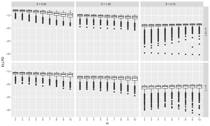
B.2 Simulation 2

The second simulation sought to investigate the effect of increasing the number of anchor points when using the anchored EM algorithm. We simulated data from models 1, 2, and 3, whose parameters are given in Table M2 and analyses of which are presented in Section M4.3 with the same prior and hyperparameter specification. From each model we generated 250 data sets of size $n=100$ and fit eight different anchor models, requiring $m_{j}=m$, $j=1,\ldots,k$, using the values of $m=1,2,3,5,7,9,10,12$. The anchor points were chosen using the anchored EM method as well as two oracle methods. The first set of oracle anchor points (random oracle points) were selected randomly from, for component $j$, the observations generated from component $j$. The second set of oracle anchor points (quantile oracle points) were chosen to be evenly-spaced percentiles from the true component densities, beginning at the 5th percentile and ending at the 95th. The model with $m=1$ uses only the 5th percentile.

The estimated ELPPD was calculated for each data set to assess the model’s predictive performance. Figure A8 shows boxplots of the ELPPD values for models 1, 2, and 3 respectively.

Figure A8: Estimated ELPPD values under the anchored EM (left), random oracle (center), and quantile oracle (right) anchor models. Rows 1, 2 and 3 give results for models 1,  2, and 3, respectively.

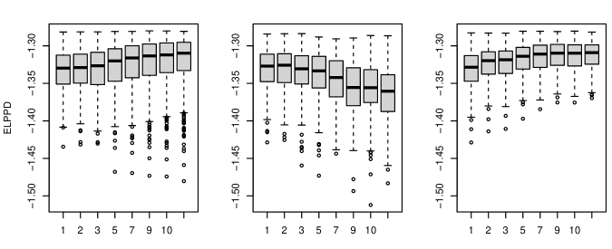
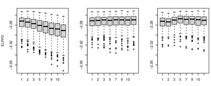
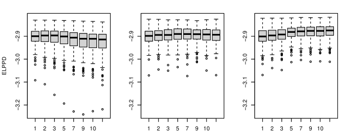
The left-hand panels display the values under anchor models specified using anchored EM, as would occur in practice. For model 1, the two-component scale mixture, the median predictive performance improves slightly as $m$ increases, but for model 2, the four-component location mixture, the performance deteriorates noticeably as the number of anchor points increases. For model 3 there is also a slight tendency for the ELPPD to decrease with higher values of $m$. In all models there is more variability in the ELPPD when $m$ is large. This pattern suggest that in models with substantial overlap among components, using many points selected by anchored EM leads to models that may introduce bias. In all models there is little apparent difference in the average ELPPD between models with $m=1$ and $m=2$.

The random and quantile oracle methods demonstrate how predictive performance changes with anchor points that represent true features of the distributions. In the random oracle models, shown in the middle panels of Figure A8 the anchor points are guaranteed to be a random sample from the component to which they are anchored. In models 2 and 3, there is little difference in the model performance as $m$ increases. In model 1, larger numbers of points lead to poorer predictive performance. The estimated ELPPD values under the quantile oracle models, are shown in the right panels of Figure A8. As $m$ increases, these points will become increasingly representative of the features of the true component densities. It is unsurprising that, for these methods, there is a slight increase in predictive performance as $m$ increases.

Appendix C Anchored EM algorithm

In this section we list the pseudo-code of the Anchored EM algorithm described in Section 3.2 of the main manuscript.

Algorithm 1 Anchored EM Algorithm

0:  Initialize $\mbox{\boldmath$\gamma$}^{0}$ and select $\epsilon>0$. Set $t=1$ and $\delta>\epsilon$.

  while  $\delta\geq\epsilon$ do

     E step: Calculate the unconstrained posterior probabilities $r_{ij}^{t}$ at the current value of $\mbox{\boldmath$\gamma$}^{t-1}$. Initialize $A^{t}=\emptyset$.

     Find $A^{t}$ to maximize $\sum_{j=1}^{k_{0}}\sum_{i\in A_{j}}r_{ij}^{t}$. Set $\widetilde{r}_{ij}^{t}=1$ and $\widetilde{r}_{il}^{t}=0,l\neq j$ for $i\in A_{j}^{t}$, $j=1,\ldots,k_{0}$. Set $\widetilde{r}_{ij}^{t}=r_{ij}^{t}$ for $i\notin A^{t},j=1,\ldots,k$. Define $q^{t}$ as in $M14$ using $\widetilde{r}_{ij}^{t}$.

     M step: Set $\mbox{\boldmath$\gamma$}^{t}=\operatorname*{arg\,max}_{\mbox{\boldmath$\gamma$}}F(\mbox{\boldmath$\gamma$},q^{t})$.

     $\delta=F(\mbox{\boldmath$\gamma$}^{t},q^{t})-F(\mbox{\boldmath$\gamma$}^{t-1},q^{t-1})$; t++.

  end while

An exact solution to the maximization of $A^{t}$ above may framed as a solution to a transportation problem where $k_{0}$ sources must be connected to $n$ destinations and the cost of connecting source $j$ to destination $i$ is $-r_{ij}^{t}$. The solution can be expressed as an $n\times k_{0}$ matrix $B$ of 0’s and 1’s, where $B_{ij}=1$ if $i\in A_{j}$, subject to the constraints $\sum_{j=1}^{k_{0}}B_{ij}\leq 1$ and $\sum_{i=1}^{n}B_{ij}=m_{j}$. The function lp.transport in the R package lpSolve (Berkelaar,, 2015) can be used to perform this step of the algorithm. Alternatively, an approximate solution may be found using, for example, Vogel’s approximation method and variants thereof (Mathirajan and Meenakshi,, 2004; Juman and Hoque,, 2015) or using the heuristic method described in the pseudo-code below.

  while $|A^{t}|<m$ do

     Find $i^{\prime},j^{\prime}=\max_{i,j:i\not\in A^{t},\;|A_{j}^{t}|<m_{j}}r_{ij}^{t}$. Set $i^{\prime}\in A_{j^{\prime}}$.

     Set $\widetilde{r}_{i^{\prime}j^{\prime}}^{t}=1$ and $\widetilde{r}_{i^{\prime}l}^{t}=0,l\neq j^{\prime}$.

  end while

Appendix D Random permutation sampler

As noted in Section 4.1, to prove that the random permutation sampler is a Gibbs sampler that generates draws from the target posterior distribution we need to show that the accepted randomly permuted draw $(\mbox{\boldmath$\gamma$},\mbox{\boldmath$\eta$})$ is in fact a draw from the distribution of $(\mbox{\boldmath$\gamma$},\mbox{\boldmath$\eta$})$ given $(\mbox{\boldmath$s$},\mbox{\boldmath$y$})$. Let $C$ be a measurable subset and let the symbol $p_{T}(\cdot|\cdot)$ denote generically a conditional density under the target posterior for the given model (either the exchangeable or the anchor model). We note first that the absolute values of the Jacobian determinants for the $k!$ permutations and their inverses are all equal to one and can therefore be ignored in the following derivation. Then we have

$$P((\mbox{\boldmath$\gamma$},\mbox{\boldmath$\eta$})\in C|\mbox{\boldmath$s$},\mbox{\boldmath$y$}) =\sum_{q=1}^{k!}\int_{\rho_{q}^{-1}(C)}\frac{p_{T}(\rho_{q}(\rho_{q}^{-1}(\mbox{\boldmath$\gamma$},\mbox{\boldmath$\eta$}))|\mbox{\boldmath$y$})}{\sum_{h=1}^{k!}p_{T}(\rho_{h}(\rho_{q}^{-1}(\mbox{\boldmath$\gamma$},\mbox{\boldmath$\eta$}))|\mbox{\boldmath$y$})}p_{T}(\rho_{q}^{-1}(\mbox{\boldmath$\gamma$},\mbox{\boldmath$\eta$})|\mbox{\boldmath$s$},\mbox{\boldmath$y$})\,d(\rho_{q}^{-1}(\mbox{\boldmath$\gamma$},\mbox{\boldmath$\eta$}))$$

$$=\sum_{q=1}^{k!}\int_{C}\frac{p_{T}(\rho_{q}(\mbox{\boldmath$\gamma$},\mbox{\boldmath$\eta$})|\mbox{\boldmath$y$})}{\sum_{h=1}^{k!}p_{T}(\rho_{h}(\mbox{\boldmath$\gamma$},\mbox{\boldmath$\eta$})|\mbox{\boldmath$y$})}p_{T}(\mbox{\boldmath$\gamma$},\mbox{\boldmath$\eta$}|\mbox{\boldmath$s$},\mbox{\boldmath$y$})\,d(\mbox{\boldmath$\gamma$},\mbox{\boldmath$\eta$})$$

$$=\int_{C}\frac{\sum_{q=1}^{k!}p_{T}(\rho_{q}(\mbox{\boldmath$\gamma$},\mbox{\boldmath$\eta$})|\mbox{\boldmath$y$})}{\sum_{h=1}^{k!}p_{T}(\rho_{h}(\mbox{\boldmath$\gamma$},\mbox{\boldmath$\eta$})|\mbox{\boldmath$y$})}p_{T}(\mbox{\boldmath$\gamma$},\mbox{\boldmath$\eta$}|\mbox{\boldmath$s$},\mbox{\boldmath$y$})\,d(\mbox{\boldmath$\gamma$},\mbox{\boldmath$\eta$})$$

$$=\int_{C}p_{T}(\mbox{\boldmath$\gamma$},\mbox{\boldmath$\eta$}|\mbox{\boldmath$s$},\mbox{\boldmath$y$})\,d(\mbox{\boldmath$\gamma$},\mbox{\boldmath$\eta$})$$

$$=P_{T}((\mbox{\boldmath$\gamma$},\mbox{\boldmath$\eta$})\in C|\mbox{\boldmath$s$},\mbox{\boldmath$y$}),$$

proving the claim. Note that for the exchangeable model all relabelings will have the same probability $1/k!$ of being selected and the algorithm reduces to the original algorithm proposed in  Frühwirth-Schnatter, (2001).

Appendix E Univariate examples with $m_{j}=2$

In this section, we revisit the univariate examples of Section (M4) using two anchor points per component. The oracle anchor points when $m_{j}=2$ are chosen as the 5th and 95th percentiles of the true component distributions. There is no minimum-entropy method demonstrated for this case.

Figure A9 shows the scaled component densities under Model 1 for the anchor models and relabeling methods. Table A7 gives posterior means of the model parameters for all methods, including the anchor models with $m_{j}=1$ as presented in the main manuscript.

Figure A9: Left panel: anchor points and true scaled component densities for model 1. Middle panel: estimated scaled component densities for the anchor models. Right panel: estimated scaled component densities for the relabeling methods and prior constraints.

Table A7: Posterior means of the component-specific parameters for Model 1.

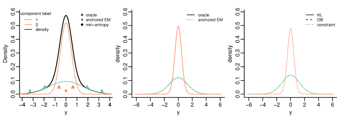
	$\theta_{1}$	$\theta_{2}$	error	time (s)
true	0	0	0	0
oracle anchors ($m_{j}=2$)	0.0004 (0.0014)	-0.0008 (0.0005)	0.0012	N/A
anchored EM ($m_{j}=2$)	-0.0004 (0.0014)	-0.0007 (0.0005)	0.0011	1.03
oracle anchors ($m_{j}=1$)	0.0010 (0.0010)	-0.0010 (0.0010)	0.0020	N/A
anchored EM ($m_{j}=1$)	-0.0027 (0.0014)	-0.0009 (0.0005)	0.0036	1.03
min-entropy($m_{j}=1$)	-0.0003 (0.0014)	-0.0006 (0.0005)	0.0009	0.50
KL	0.0005 (0.0013)	-0.0008 (0.0005)	0.0013	1102.78
DB	0.0005 (0.0013)	-0.0008 (0.0005)	0.0013	547.59
constraint	0.0005 (0.0013)	-0.0008 (0.0005)	0.0013	N/A
	$\sigma_{1}$	$\sigma_{2}$	error
true	1.5	0.5	0
oracle anchors ($m_{j}=2$)	1.356 (0.0013)	0.485 (0.0005)	0.1593
anchored EM ($m_{j}=2$)	1.333 (0.0013)	0.470 (0.0006)	0.1973
oracle anchors ($m_{j}=1$)	0.867 (0.0035)	0.866 (0.0035)	0.9988
anchored EM ($m_{j}=1$)	1.320 (0.0013)	0.467 (0.0006)	0.2125
min-entropy ($m_{j}=1$)	1.320 (0.0013)	0.468 (0.0006)	0.2122
KL	1.307 (0.0013)	0.464 (0.0005)	0.2293
DB	1.307 (0.0013)	0.464 (0.0006)	0.2293
constraint	1.733 (0.0013)	0.220 (0.0005)	0.5129
	$\eta_{1}$	$\eta_{2}$	error
true	0.35	0.65	0
oracle anchors ($m_{j}=2$)	0.395 (0.0008)	0.605 (0.0008)	0.0907
anchored EM ($m_{j}=2$)	0.418 (0.0008)	0.582 (0.0008)	0.1363
oracle anchors ($m_{j}=1$)	0.501 (0.0009)	0.499 (0.0009)	0.3020
anchored EM ($m_{j}=1$)	0.430 (0.0009)	0.570 (0.0009)	0.1594
min-entropy ($m_{j}=1$)	0.428 (0.0009)	0.572 (0.0009)	0.1568
KL	0.439 (0.0009)	0.561 (0.0009)	0.1781
DB	0.439 (0.0009)	0.561 (0.0009)	0.1782
constraint	0.439 (0.0009)	0.561 (0.0009)	0.1781

Figure A10 shows the scaled component densities under Model 2 and Table A8 gives posterior means of the model parameters for all methods, including the anchor models with $m_{j}=1$ as presented in the main manuscript.

Figure A10: Left panel: anchor points and true scaled component densities for model 2. Middle panel: estimated scaled component densities for the anchor models. Right panel: estimated scaled component densities for the relabeling methods and prior constraints.

The results for Model 3 are shown in Figure A11 and Table A9.

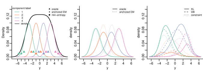
In Model 1, the anchor models with two anchor points provide parameter estimates with higher accuracy than the ones with one anchor points. This improvement is, however, not seen for all parameters in Model 2 and Model 3. The anchored EM model with $m_{j}=1$ provides more accurate estimates of both $\theta$ and $\eta$ for Model 2, although $m_{j}=2$ produces better estimates of $\sigma$. For Model 3, the anchored EM model is more accurate with $m_{j}=1$ than with $m_{j}=2$.

Table A8: Posterior means of the component-specific parameters for Model 2.

	$\theta_{1}$	$\theta_{2}$	$\theta_{3}$	$\theta_{4}$	error	time (s)
true	-3	-1	1	3	0
oracle anchors ($m_{j}=2$)	-2.802 (0.0037)	-0.978 (0.0059)	0.979 (0.0057)	2.800 (0.0038)	0.442	N/A
anchored EM ($m_{j}=2$)	-3.104 (0.0051)	-1.061 (0.0050)	1.138 (0.0050)	3.140 (0.0051)	0.443	21.39
oracle anchors ($m_{j}=1$)	-2.819 (0.0049)	-0.960 (0.0072)	0.956 (0.0072)	2.818 (0.0049)	0.448	N/A
anchored EM ($m_{j}=1$)	-2.983 (0.0069)	-0.960 (0.0073)	0.997 (0.0073)	2.997 (0.0068)	0.063	24.87
min-entropy ($m_{j}=1$)	-2.967 (0.0116)	-1.653 (0.0095)	1.965 (0.0088)	2.864 (0.0134)	1.786	10.37
KL	-2.208 (0.0078)	-0.942 (0.0376)	1.288 (0.0090)	1.864 (0.0318)	2.274	6134.31
DB	-2.536 (0.0141)	-0.259 (0.0393)	0.278 (0.0136)	2.520 (0.0199)	2.408	159.00
constraint	-3.477 (0.0230)	-1.039 (0.0129)	1.027 (0.0127)	3.492 (0.0225)	1.035	N/A
	$\sigma_{1}$	$\sigma_{2}$	$\sigma_{3}$	$\sigma_{4}$	error
true	1	1	1	1	0
oracle anchors ($m_{j}=2$)	1.109 (0.0020)	1.257 (0.0030)	1.259 (0.0031)	1.108 (0.0020)	0.7333
anchored EM ($m_{j}=2$)	1.011 (0.0020)	0.954 (0.0027)	0.945 (0.0026)	1.001 (0.0020)	0.1135
oracle anchors ($m_{j}=1$)	1.024 (0.0026)	1.067 (0.0041)	1.063 (0.0039)	1.026 (0.0025)	0.1805
anchored EM ($m_{j}=1$)	1.074 (0.0025)	0.984 (0.0031)	0.984 (0.0032)	1.069 (0.0025)	0.1752
min-entropy ($m_{j}=1$)	1.121 (0.0040)	1.089 (0.0036)	1.042 (0.0034)	1.168 (0.0043)	0.4192
KL	1.243 (0.0037)	0.699 (0.0069)	1.497 (0.0023)	0.766 (0.0068)	1.270
DB	1.071 (0.0033)	0.687 (0.0028)	1.476 (0.0050)	0.970 (0.0031)	0.8893
constraint	0.981 (0.0038)	1.123 (0.0048)	1.122 (0.0048)	0.979 (0.0038)	0.2848
	$\eta_{1}$	$\eta_{2}$	$\eta_{3}$	$\eta_{4}$	error
true	0.25	0.25	0.25	0.25	0
oracle anchors ($m_{j}=2$)	0.245 (0.0007)	0.254 (0.0009)	0.255 (0.0009)	0.246 (0.0007)	0.0181
anchored EM ($m_{j}=2$)	0.236 (0.0010)	0.269 (0.0010)	0.266 (0.0010)	0.229 (0.0009)	0.0702
oracle anchors ($m_{j}=1$)	0.247 (0.0011)	0.252 (0.0013)	0.251 (0.0013)	0.250 (0.0010)	0.0059
anchored EM ($m_{j}=1$)	0.255 (0.0012)	0.247 (0.0012)	0.247 (0.0012)	0.251 (0.0012)	0.0124
min-entropy ($m_{j}=1$)	0.222 (0.0016)	0.283 (0.0016)	0.263 (0.0014)	0.232 (0.0018)	0.0923
KL	0.353 (0.0015)	0.075 (0.0006)	0.459 (0.0017)	0.114 (0.0008)	0.6230
DB	0.273 (0.0015)	0.077 (0.0007)	0.427 (0.0022)	0.223 (0.0014)	0.4010
constraint	0.224 (0.0017)	0.276 (0.0020)	0.277 (0.0019)	0.224 (0.0017)	0.1047

Figure A11: Left panel: anchor points and true scaled component densities for model 3. Middle panel: estimated scaled component densities for the anchor models. Right panel: estimated scaled component densities for the relabeling methods and prior constraints.

Table A9: Posterior means of the component-specific parameters for Model 3.

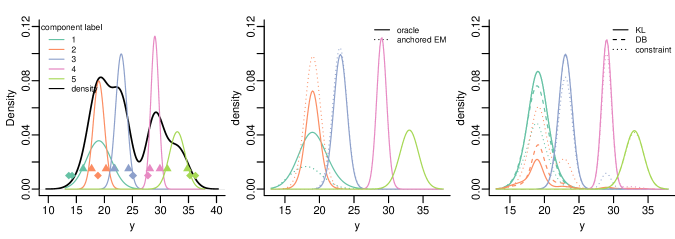
	$\theta_{1}$	$\theta_{2}$	$\theta_{3}$	$\theta_{4}$	$\theta_{5}$	error	time (s)
true	19	19	23	29	33	0
oracle anchors ($m_{j}=2$)	18.990 (0.0053)	19.012 (0.0020)	23.023 (0.0011)	29.007 (0.0006)	32.993 (0.0016)	0.059	N/A
anchored EM ($m_{j}=2$)	16.822 (0.0224)	19.044 (0.0015)	22.954 (0.0012)	29.006 (0.0006)	32.990 (0.0016)	2.284	16.11
oracle anchors ($m_{j}=1$)	18.955 (0.0049)	18.958 (0.0049)	23.030 (0.0014)	29.006 (0.0006)	32.990 (0.0016)	0.135	N/A
anchored EM ($m_{j}=1$)	17.273 (0.0290)	19.049 (0.0019)	22.975 (0.0014)	29.006 (0.0006)	32.991 (0.0016)	1.816	16.60
min-entropy ($m_{j}=1$)	18.948 (0.0014)	23.011 (0.0010)	29.006 (0.0006)	33.031 (0.0056)	33.838 (0.0100)	14.94	10.56
KL	19.086 (0.0026)	20.087 (0.0868)	23.028 (0.0016)	29.005 (0.0007)	32.992 (0.0018)	1.215	986.31
DB	18.799 (0.0062)	20.335 (0.0831)	23.065 (0.0044)	29.007 (0.0007)	32.994 (0.0018)	1.613	285.12
constraint	17.848 (0.0255)	20.062 (0.0287)	23.856 (0.0351)	29.266 (0.0117)	33.167 (0.0150)	3.504	N/A
	$\sigma_{1}$	$\sigma_{2}$	$\sigma_{3}$	$\sigma_{4}$	$\sigma_{5}$	error
true	2.236	1	1	0.7071	1.414	0
oracle anchors ($m_{j}=2$)	2.059 (0.0028)	1.018 (0.0020)	0.973 (0.0008)	0.717 (0.0005)	1.363 (0.0012)	0.284
anchored EM ($m_{j}=2$)	1.377 (0.0067)	1.125 (0.0031)	1.023 (0.0009)	0.719 (0.0005)	1.364 (0.0012)	1.070
oracle anchors $(m_{j}=1)$	1.371 (0.0048)	1.380 (0.0048)	0.973 (0.0010)	0.719 (0.0005)	1.364 (0.0012)	1.334
anchored EM $(m_{j}=1)$	1.490 (0.0081)	1.073 (0.0042)	1.011 (0.0009)	0.719 (0.0005)	1.363 (0.0012)	0.892
min-entropy $(m_{j}=1)$	1.606 (0.0010)	1.011 (0.0007)	0.718 (0.0005)	1.067 (0.0025)	1.134 (0.0037)	1.563
KL	1.581 (0.0023)	0.986 (0.0062)	0.973 (0.0013)	0.716 (0.0011)	1.358 (0.0007)	0.760
DB	1.579 (0.0036)	0.989 (0.0052)	0.971 (0.0012)	0.716 (0.0006)	1.358 (0.0013)	0.761
constraint	1.322 (0.0049)	1.273 (0.0060)	0.934 (0.0024)	0.746 (0.0018)	1.338 (0.0019)	1.368
	$\eta_{1}$	$\eta_{2}$	$\eta_{3}$	$\eta_{4}$	$\eta_{5}$	error
true	0.2	0.2	0.25	0.2	0.15	0
oracle anchors ($m_{j}=2$)	0.219 (0.0006)	0.187 ( NA)	0.244 (0.0003)	0.201 (0.0001)	0.149 (0.0001)	0.0405
anchored EM ($m_{j}=2$)	0.094 (0.0015)	0.286 (0.0013)	0.269 (0.0003)	0.201 (0.0001)	0.149 (0.0001)	0.2134
oracle anchors $(m_{j}=1)$	0.201 (0.0008)	0.204 (0.0008)	0.245 (0.0003)	0.201 (0.0001)	0.149 (0.0001)	0.0127
anchored EM $(m_{j}=1)$	0.132 (0.0021)	0.255 (0.0019)	0.264 (0.0003)	0.201 (0.0001)	0.149 (0.0001)	0.1387
min-entropy $(m_{j}=1)$	0.392 (0.0002)	0.255 (0.0002)	0.200 (0.0002)	0.088 (0.0004)	0.064 (0.0004)	0.4954
KL	0.334 (0.0011)	0.074 (0.0008)	0.246 (0.0005)	0.198 (0.0002)	0.147 (0.0002)	0.2688
DB	0.303 (0.0016)	0.106 (0.0013)	0.245 (0.0005)	0.198 (0.0002)	0.147 (0.0002)	0.2063
constraint	0.189 (0.0023)	0.253 (0.0012)	0.228 (0.0010)	0.186 (0.0007)	0.143 (0.0003)	0.1060

Appendix F Analysis of the SisFall data

This section provides additional details on the data analysis example presented in Section 5 of the main manuscript.

Data.

The full SisFall data set collected by Sucerquia et al., (2017), with additional details on the experimental procedure, is available at http://sistemic.udea.edu.co/en/research/projects/english-falls/.

Additional tables.

Table A10 gives posterior means of $\mbox{\boldmath$\theta$}_{j}$ for each mixture component. Table A11 gives the full table of posterior allocation probabilities for each of the activities considered in the analysis. Activities beginning with “D” are ADLs and activities beginning with “F” are falls.

Table A10: Posterior means of $\mbox{\boldmath$\theta$}_{j}$ for each component from the SisFall data.

Component	1	2	3	4	5
$\log(\max_{t}SMV_{t})$	5.769	7.304	7.169	6.972	6.366
$\log(\min_{t}SMV_{t})$	5.323	3.661	1.686	4.626	3.795
$\log(\max_{t}|SMV_{t}-SMV_{t-1}|)$	3.162	5.963	5.802	5.021	3.979

Table A11: Posterior allocation probabilities for selected activities in the SisFall dataset.

Activity	Component
	1	2	3	4	5
D01 Walking slowly	0.099	0.008	0.000	0.490	0.403
D02 Walking quickly	0.000	0.086	0.000	0.066	0.848
D03 Jogging slowly	0.000	0.000	1.000	0.000	0.000
D04 Jogging quickly	0.000	0.011	0.989	0.000	0.000
D05 Walking upstairs and downstairs slowly	0.059	0.027	0.000	0.887	0.027
D06 Walking upstairs and downstairs quickly	0.000	0.796	0.188	0.000	0.016
D07 Slowly sit in a half height chair, wait a moment, and up slowly	0.981	0.000	0.000	0.006	0.013
D08 Quickly sit in a half height chair, wait a moment, and up quickly	0.000	0.019	0.001	0.024	0.956
D09 Slowly sit in a low height chair, wait a moment, and up slowly	0.245	0.050	0.000	0.575	0.131
D10 Quickly sit in a low height chair, wait a moment, and up quickly	0.001	0.042	0.001	0.148	0.808
D11 Sitting a moment, trying to get up, and collapse into a chair	0.000	0.541	0.003	0.454	0.002
D12 Sitting a moment, lying slowly, wait a moment, and sit again	0.938	0.020	0.000	0.035	0.007
D13 Sitting a moment, lying quickly, wait a moment, and sit again	0.173	0.110	0.000	0.695	0.022
D14 Being on one’s back change to lateral position, wait a moment, and change to one’s back	0.942	0.001	0.000	0.038	0.019
D15 Standing, slowly bending at knees, and getting up	0.978	0.000	0.000	0.010	0.012
D16 Standing, slowly bending without bending knees, and getting up	0.986	0.000	0.000	0.008	0.005
D17 Standing, get into a car, remain seated and get out of the car	0.797	0.003	0.000	0.156	0.045
D18 Stumble while walking	0.000	0.957	0.003	0.040	0.000
D19 Gently jump without falling (trying to reach a high object)	0.000	0.308	0.033	0.000	0.658
F01 Fall forward while walking caused by a slip	0.000	0.915	0.001	0.084	0.000
F02 Fall backward while walking caused by a slip	0.000	0.302	0.001	0.697	0.000
F03 Lateral fall while walking caused by a slip	0.000	0.250	0.000	0.750	0.000
F04 Fall forward while walking caused by a trip	0.000	0.938	0.001	0.061	0.000
F05 Fall forward while jogging caused by a trip	0.000	0.799	0.201	0.000	0.000
F06 Vertical fall while walking caused by fainting	0.000	0.058	0.000	0.942	0.000
F07 Fall while walking, with use of hands in a table to dampen fall, caused by fainting	0.000	0.211	0.001	0.788	0.000
F08 Fall forward when trying to get up	0.001	0.586	0.001	0.412	0.000
F09 Lateral fall when trying to get up	0.000	0.074	0.000	0.926	0.000
F10 Fall forward when trying to sit down	0.000	0.609	0.001	0.390	0.000
F11 Fall backward when trying to sit down	0.000	0.230	0.002	0.760	0.008
F12 Lateral fall when trying to sit down	0.000	0.239	0.001	0.759	0.000
F13 Fall forward while sitting, caused by fainting or falling asleep	0.014	0.726	0.001	0.124	0.135
F14 Fall backward while sitting, caused by fainting or falling asleep	0.001	0.527	0.003	0.467	0.002
F15 Lateral fall while sitting, caused by fainting or falling asleep	0.000	0.439	0.001	0.561	0.000

References

- Abney, (2004) Abney, S. (2004). Understanding the Yarowsky algorithm. Comput. Linguist., 30(3):365–395.
- Albert et al., (2012) Albert, M. V., Kording, K., Herrmann, M., and Jayaraman, A. (2012). Fall classification by machine learning using mobile phones. PLOS ONE, 7:1–6.
- Bardenet et al., (2012) Bardenet, R., Cappe, O., Fort, G., and Kegl, B. (2012). Adaptive Metropolis with online relabeling. In Lawrence, N. D. and Girolami, M., editors, Proceedings of the Fifteenth International Conference on Artificial Intelligence and Statistics, volume 22 of Proceedings of Machine Learning Research, pages 91–99, La Palma, Canary Islands. PMLR.
- Berk, (1966) Berk, R. H. (1966). Limiting behavior of posterior distributions when the model is incorrect. 37:51–58.
- Berkelaar, (2015) Berkelaar, M. (2015). lpSolve: Interface to ‘Lp_solve’ v. 5.5 to Solve Linear/Integer Programs. R package version 5.6.13.
- Bourke and Lyons, (2008) Bourke, A. and Lyons, G. (2008). A threshold-based fall-detection algorithm using a bi-axial gyroscope sensor. Medical Engineering & Physics, 30:84 – 90.
- Casilari et al., (2017) Casilari, E., Santoyo-Ramón, J.-A., and Cano-García, J.-M. (2017). Analysis of public datasets for wearable fall detection systems. Sensors, 17.
- Celeux et al., (2000) Celeux, G., Hurn, M., and Robert, C. P. (2000). Computational and inferential difficulties with mixture posterior distributions. Journal of the American Statistical Association, 95:957–970.
- Chung et al., (2004) Chung, H., Loken, E., and Schafer, J. L. (2004). Difficulties in drawing inferences with finite-mixture models. The American Statistician, 58:152–158.
- Cooley and MacEachern, (1999) Cooley, C. A. and MacEachern, S. N. (1999). Prior elicitation in the classification problem. The Canadian Journal of Statistics / La Revue Canadienne de Statistique, 27:299–313.
- Diebolt and Robert, (1994) Diebolt, J. and Robert, C. P. (1994). Estimation of finite mixture distributions through Bayesian sampling. Journal of the Royal Statistical Society. Series B (Statistical Methodology), 56:363–375.
- Egidi et al., (2018) Egidi, L., Pappadà, R., Pauli, F., and Torelli, N. (2018). Relabelling in bayesian mixture models by pivotal units. Statistics and Computing, 28:957–969.
- Flegal et al., (2020) Flegal, J. M., Hughes, J., Vats, D., and Dai, N. (2020). mcmcse: Monte Carlo Standard Errors for MCMC. Riverside, CA, Denver, CO, Coventry, UK, and Minneapolis, MN. R package version 1.4-1.
- Frühwirth-Schnatter, (2001) Frühwirth-Schnatter, S. (2001). Markov chain Monte Carlo estimation of classical and dynamic switching and mixture models. Journal of the American Statistical Association, 96:194–209.
- Frühwirth-Schnatter, (2006) Frühwirth-Schnatter, S. (2006). Finite mixture and Markov switching models. Springer.
- Ganchev et al., (2008) Ganchev, K., Taskar, B., and ao Gama, J. (2008). Expectation maximization and posterior constraints. In Platt, J. C., Koller, D., Singer, Y., and Roweis, S. T., editors, Advances in Neural Information Processing Systems 20, pages 569–576. Curran Associates, Inc.
- Gelman et al., (2014) Gelman, A., Hwang, J., and Vehtari, A. (2014). Understanding predictive information criteria for Bayesian models. Statistics and Computing, 24:997–1016.
- Genovese and Wasserman, (2000) Genovese, C. R. and Wasserman, L. (2000). Rates of convergence for the Gaussian mixture sieve. The Annals of Statistics, 28:1105–1127.
- Geweke, (2007) Geweke, J. (2007). Interpretation and inference in mixture models: Simple MCMC works. Computational Statistics & Data Analysis, 51(7):3529 – 3550.
- Grazian and Robert, (2018) Grazian, C. and Robert, C. P. (2018). Jeffreys priors for mixture estimation: Properties and alternatives. Computational Statistics & Data Analysis, 121:149 – 163.
- Jasra et al., (2005) Jasra, A., Holmes, C. C., and Stephens, D. A. (2005). Markov chain Monte Carlo methods and the label switching problem in Bayesian mixture modeling. Statistical Science, 20:50–67.
- Juman and Hoque, (2015) Juman, Z. and Hoque, M. (2015). An efficient heuristic to obtain a better initial feasible solution to the transportation problem. Applied Soft Computing, 34:813 – 826.
- Kunkel, (2018) Kunkel, D. (2018). Anchored Bayesian Gaussian Mixture Models. PhD thesis, The Ohio State University.
- Kunkel and Peruggia, (2019) Kunkel, D. and Peruggia, M. (2019). Statistical inference with anchored Bayesian mixture of regressions models: A case study analysis of allometric data. arXiv preprint, arXiv:1905.04389.
- Li and Fan, (2016) Li, H. and Fan, X. (2016). A pivotal allocation-based algorithm for solving the label-switching problem in Bayesian mixture models. Journal of Computational and Graphical Statistics, 25:266–283.
- Lücke, (2016) Lücke, J. (2016). Truncated variational expectation maximization. arXiv preprint, arXiv:1610.03113.
- Maechler, (2019) Maechler, M. (2019). nor1mix: Normal aka Gaussian (1-d) Mixture Models. R package version 1.3-0.
- Marin et al., (2005) Marin, J.-M., Mengersen, K., and Robert, C. P. (2005). Bayesian modelling and inference on mixtures of distributions. In Dey, D. and Rao, C., editors, Bayesian Thinking Modeling and Computation, volume 25 of Handbook of Statistics, pages 459 – 507. Elsevier.
- Marin and Robert, (2014) Marin, J.-M. and Robert, C. P. (2014). Bayesian essentials with R. Springer.
- Mathirajan and Meenakshi, (2004) Mathirajan, M. and Meenakshi, B. (2004). Experimental analysis of some variants of Vogel’s approximation method. Asia - Pacific Journal of Operational Research, 21(4):447–462.
- Neal and Hinton, (1998) Neal, R. M. and Hinton, G. E. (1998). A View of the EM Algorithm that Justifies Incremental, Sparse, and other Variants, pages 355–368. Springer Netherlands, Dordrecht.
- Norets and Pelenis, (2012) Norets, A. and Pelenis, J. (2012). Bayesian modeling of joint and conditional distributions. Journal of Econometrics, 168:332–346.
- Papastamoulis, (2016) Papastamoulis, P. (2016). label.switching: An R package for dealing with the label switching problem in MCMC outputs. Journal of Statistical Software, Code Snippets, 69:1–24.
- Papastamoulis and Iliopoulos, (2010) Papastamoulis, P. and Iliopoulos, G. (2010). An artificial allocations based solution to the label switching problem in bayesian analysis of mixtures of distributions. Journal of Computational and Graphical Statistics, 19(2):313–331.
- Richardson and Green, (1997) Richardson, S. and Green, P. J. (1997). On Bayesian analysis of mixtures with an unknown number of components (with discussion). Journal of the Royal Statistical Society: Series B (Statistical Methodology), 59:731–792.
- Rodriguez and Walker, (2014) Rodriguez, C. E. and Walker, S. G. (2014). Label switching in Bayesian mixture models. Journal of Computational and Graphical Statistics, 23:25–45.
- Roeder, (1990) Roeder, K. (1990). Density estimation with confidence sets exemplified by superclusters and voids in the galaxies. Journal of the American Statistical Association, 85:617–624.
- Roeder and Wasserman, (1997) Roeder, K. and Wasserman, L. (1997). Practical Bayesian density estimation using mixtures of normals. Journal of the American Statistical Association, 92:894–902.
- Rossi, (2014) Rossi, P. E. (2014). Bayesian Non- and Semi-parametric Methods and Applications. Princeton University Press.
- Stephens, (2000) Stephens, M. (2000). Dealing with label switching in mixture models. Journal of the Royal Statistical Society. Series B (Statistical Methodology), 62:795–809.
- Sucerquia et al., (2017) Sucerquia, A., López, J. D., and Vargas-Bonilla, J. F. (2017). SisFall: A fall and movement dataset. Sensors, 17.
- Wasserman, (2000) Wasserman, L. (2000). Asymptotic inference for mixture models by using data-dependent priors. Journal of the Royal Statistical Society: Series B (Statistical Methodology), 62:159–180.
- Yarowsky, (1995) Yarowsky, D. (1995). Unsupervised word sense disambiguation rivaling supervised methods. In Proceedings of the 33rd Annual Meeting on Association for Computational Linguistics, ACL ’95, pages 189–196, Stroudsburg, PA, USA. Association for Computational Linguistics.