Multiple Causal Inference with Latent Confounding

Abstract

Causal inference from observational data requires assumptions. These assumptions range from measuring confounders to identifying instruments. Traditionally, causal inference assumptions have focused on estimation of effects for a single treatment. In this work, we construct techniques for estimation with multiple treatments in the presence of unobserved confounding. We develop two assumptions based on shared confounding between treatments and independence of treatments given the confounder. Together, these assumptions lead to a confounder estimator regularized by mutual information. For this estimator, we develop a tractable lower bound. To recover treatment effects, we use the residual information in the treatments independent of the confounder. We validate on simulations and an example from clinical medicine.

1 Introduction

Causal inference aims to estimate the effect one variable has on another. Causal inferences form the heart of inquiry in many domains, including estimating the value of giving a medication to a patient, understanding the influence of genetic variations on phenotypes, and measuring the impact of job training programs on income.

Assumption-free causal inferences rely on randomized experimentation (Cook et al.,, 2002; Pearl et al.,, 2009). Randomized experiments break the relationship between the intervention variable (the treatment) and variables that could alter both the treatment and the outcome—confounders. Though powerful, randomized experimentation fails to make use of large collections of non-randomized observational data (like electronic health records in medicine) and is inapplicable where broad experimentation is infeasible (like in human genetics). The counterpart to experimentation is causal inference from observational data. Causal inference from observational data requires assumptions. These assumptions include measurement of all confounders (Rosenbaum and Rubin,, 1983), the presence of external randomness that partially controls treatment (Angrist et al.,, 1996), and structural assumptions on the randomness (Hoyer et al.,, 2009).

Though causal inference from observational data has been used in many domains, the assumptions that underlie these inferences focus on estimation of a causal effect with a single treatment. But many real-world applications consist of multiple treatments. For example, the effects of genetic variation on various phenotypes (Consortium et al.,, 2007) or the effects of medications from order sets in clinical medicine (O’connor et al.,, 2009) consist of causal problems with multiple treatments rather than a single treatment. Considering multiple treatments make new kinds of assumptions possible.

We formalize multiple causal inference, a collection of causal inference problems with multiple treatments and a single outcome. We develop a set of assumptions under which causal effects can be estimated when confounders are unmeasured. Two assumptions form the starting point: that the treatments share confounders, and that given the shared confounder, all of the treatments are independent. This kind of shared confounding structure can be found in many domains such as genetics.

One class of estimators for unobserved confounders take in treatments and output a noisy estimate of the unmeasured confounders. Estimators for multiple causal inference should respect the assumptions of the problem. To respect shared confounding, the information between the confounder and a treatment given the rest of the treatments should be minimal. However, forcing this information to zero makes the confounder independent of the treatments. This can violate the assumption of independence given the shared confounder. This tension parallels that between underfitting and overfitting. Confounders with low information underfit, while confounders with high information memorize the treatments and overfit.

To resolve the tension between the two assumptions, we develop a regularizer based on the additional mutual information each treatment contributes to the estimated confounder given the rest of the treatments. We develop an algorithm that estimates the confounder by simultaneously minimizing the reconstruction error of the treatments, while regularizing the additional mutual information. The stochastic confounder estimator can include complex nonlinear transformations of the treatments. In practice, we use neural networks. The additional mutual information is intractable, so we build a lower bound called the multiple causal lower bound (mclbo).

The last step in building a causal estimator is to build the outcome model. Traditional outcome models regress the confounders and treatments to the outcome (Morgan and Winship,, 2014). However, since the confounder estimate is a stochastic function of the treatments, it contains no new information about the response over the treatments—a regression on both the estimated confounder and treatments can ignore the estimated confounder. Instead, we build regression models using the residual information in the treatments and develop an estimator to compute these residuals. We call the entire causal estimation process multiple causal estimation via information (mcei). Under technical conditions, we show that the causal estimates converge to the true causal effects as the number of treatments and examples grow. The assumptions we develop strengthen the foundation for existing causal estimation with unobserved confounders such as causal estimation with linear mixed models (lmms) (Kang et al.,, 2010; Lippert et al.,, 2011).

We demonstrate mcei on a large simulation study. Though traditional methods like principal component analysis (pca) adjustment (Yu et al.,, 2006) closely approximate the family of techniques we describe, we find that our approach more accurately estimates the causal effects, even when the confounder dimensionality is misspecified. Finally, we apply the mclbo to control for confounders in a medical prediction problem on health records from the Multiparameter Intelligent Monitoring in Intensive Care (mimic iii) clinical database (Johnson et al.,, 2016). We show the recovered effects match the literature.

Related Work.

Causal inference has a long history in many disciplines including statistics, computer science, and econometrics. A full review is outside of the scope of this article, however, we highlight some of recent advances in building flexible causal models. Wager and Athey, (2017) develop random forests to capture variability in treatment effects (Wager and Athey,, 2017). Hill, (2011) uses Bayesian nonparametric methods to model the outcome response. Louizos et al., (2017) build flexible latent variables to correct for confounding when proxies of confounders are measured, rather than the confounders themselves. Johansson et al., (2016); Shalit et al., (2017) develop estimators with theoretical guarantees by building representations that penalize differences in confounder distributions between the treated and untreated.

The above approaches focus on building estimators for single treatments, where either the confounder or a non-treatment proxy is measured. In contrast, computational genetics has developed a variety of methods to control for unmeasured confounding in genome-wide association studies (gwas). Genome-wide association studies have multiple treatments in the form of genetic variations across multiple sites. Yu et al., (2006); Kang et al., (2010); Lippert et al., (2011) estimate kinship matrices between individuals using a subset of the genetic variations, then fit a lmm where the kinship provides the covariance for random effects. Song et al., (2015) adjust for confounding via factor analysis on discrete variables and use inverse regression to estimate individual treatment effects. Tran and Blei, (2017) build implicit models for genome-wide association studies and describe general implicit causal models in the same vein as Kocaoglu et al., (2017). A formulation of multiple causal inference was also proposed by (Wang and Blei,, 2018); they take a model-based approach in the potential outcomes framework that leverages predictive checks.

Our grounding for multiple causal inference complements this earlier work. We develop the two assumptions of shared confounding and of independence given shared confounders. We introduce a mutual information based regularizer that trades off between these assumptions. Earlier work estimates confounders by choosing their dimensionality (e.g., number of PCA components) to not overfit. This matches the flavor of the estimator we develop. Lastly, we describe how residual information must be used to fit complex outcome models.

2 Multiple Causal Inference

The trouble with causal inference from observational data lies in confounders, variables that affect both treatments and outcome. The problem is that the observed statistical relationship between the treatment and outcome may be partially or completely due to the confounder. Randomizing the treatment breaks the relationship between the treatment and confounder, rendering the observed statistical relationship causal. But the lack of randomized data necessitates assumptions to control for potential confounders. These assumptions have focused on causal estimation with a single treatment and a single outcome. In real-world settings such as in genetics and medicine, there are multiple treatments. We now define the multiple causal inference problem, detail assumptions for multiple causal inference, and develop new estimators for the causal effects given these assumptions.

Multiple causal inference consists of a collection of causal inference problems. Consider a set of $T$ treatments indexed by $i$ denoted $t_{i}$ and an outcome $y$. The goal of multiple causal inference is to compute the joint casual effect of intervening on treatments by setting them to ${\boldsymbol{\mathbf{t}}}^{*}$

$$\mathbb{E}[y\,|\,do({\boldsymbol{\mathbf{t}}}={\boldsymbol{\mathbf{t}}}^{*})]$$

For example, $t_{i}$ could be the $i$th medication for a disease given to a patient and $y$ could be the severity of that disease. The patient’s unmeasured traits induce a relationship between the treatments and the outcome. The goal of multiple causal inference is to simultaneously estimate the causal effects for all $T$ treatments. We develop two assumptions under which these causal effects can be estimated in the presence of unobserved confounders and later show that the estimation error gets small as the number of treatments and observations gets large.

Shared Confounding.

The first assumption we make to identify multiple causal effects is that of shared confounder(s). The shared confounder assumption posits that the confounder is shared across all of the treatments. Under this assumption, each treatment provides a view on the shared confounder. With sufficient views, the confounder becomes unveiled. Shared confounding is a natural assumption in many problems. For example, in gwas, treatments are genetic variations and the outcome is a phenotype. Due to correlations in genetic variations caused by ancestry, the treatments share confounding.

Independence Given Unobserved Confounders.

The shared confounding assumption does not identify the causal effects since there can be direct causal links between treatments $t_{i}$ and $t_{j}$. In the presence of these links, we cannot get a clear view of the shared confounder because the dependence between $t_{i}$ and $t_{j}$ may be due either to confounding or to the direct link between the pair of treatments. To address this, we assume that treatments are independent given confounders. In the discussion, we explore strategies to loosen this assumption.

Implied Model.

We developed two assumptions: shared confounding and independence given the confounder. Together, these assumptions imply the existence of an unmeasured variable ${\boldsymbol{\mathbf{z}}}$ with some unknown distribution such that when conditioned on, the treatments become independent:

Proposition 1

Let ${\boldsymbol{\mathbf{\epsilon}}}$ be independent noise terms, and $f,g,h$ be functions. Then, shared confounding and independence given unobserved confounding imply a generative process for the data that is

$${\boldsymbol{\mathbf{z}}} =f({\boldsymbol{\mathbf{\epsilon}}}_{\boldsymbol{\mathbf{z}}}),\quad t_{i}=h_{i}({\boldsymbol{\mathbf{\epsilon}}}_{i},{\boldsymbol{\mathbf{z}}}),\quad y=g({\boldsymbol{\mathbf{\epsilon}}}_{y},{\boldsymbol{\mathbf{z}}},t_{1},...,t_{T}).$$ (1)

We require that (i) any given value of the treatments, $t_{i}$, be expressible as a function of the treatment noise, ${\boldsymbol{\mathbf{\epsilon}}}_{i}$, given any value of the confounder, ${\boldsymbol{\mathbf{z}}}$. Also, we require that (ii) the outcome, $y$, be a non-degenerate function of the treatment noise, ${\boldsymbol{\mathbf{\epsilon}}}_{i}$, via the treatments, $t_{i}$. This requirement ensures that there is a one-to-one mapping between $y=g({\boldsymbol{\mathbf{\epsilon}}}_{y},{\boldsymbol{\mathbf{z}}},t_{1},...,t_{T})$ and the rewritten version $y=g({\boldsymbol{\mathbf{\epsilon}}}_{y},{\boldsymbol{\mathbf{z}}},h_{1}({\boldsymbol{\mathbf{\epsilon}}}_{1},{\boldsymbol{\mathbf{z}}}),...,h_{T}({\boldsymbol{\mathbf{\epsilon}}}_{T},{\boldsymbol{\mathbf{z}}}))$.

If the model in Equation 1 were explicitly given, posterior inference would reveal the causal effects up to the posterior variance of the latent confounder. In general the model is not known, thus the goal is to build a flexible estimator for a broad class of problems.

3 Unobserved Confounder Estimation in Multiple Causal Inference

We develop an estimator for the unobserved confounder in multiple causal inference without directly specifying a generative model. This estimator finds the confounder that reconstructs each treatment given the other treatments. The estimator works via information-based regularization and cross-validation in a way that is agnostic to the particular functional form of the estimator. We present a pair of lower bounds to estimate the confounder.

Confounder Estimation.

The most general form of a confounder estimator is a function that takes the following as input: noise ${\boldsymbol{\mathbf{\epsilon}}}$, parameters ${\boldsymbol{\mathbf{\theta}}}$, treatments ${\boldsymbol{\mathbf{t}}}_{j}$, and outcome $y_{j}$. Using the outcome without extra assumptions is inherently ambiguous. The ambiguity lies in how much of $y_{j}$ is retained in ${\boldsymbol{\mathbf{z}}}_{j}$. The only statistics we observe about $y$ come from $y$ or its cross statistics with ${\boldsymbol{\mathbf{t}}}$. From eq. 1, we know that the cross statistics provide a way to estimate ${\boldsymbol{\mathbf{z}}}$ the confounder. However, since the outcome depends on the treatments, cross statistics between the treatment and outcome could either be from the confounder or from the direct relationship between the treatments and outcome. This ambiguity cannot be resolved without further assumptions like assuming a model. Therefore we focus on estimating the unobserved confounder without using the outcome, where the outcome has been marginalized.

A generic stochastic confounder estimator with marginalized outcome is a stochastic function of the treatments controlled by parameters ${\boldsymbol{\mathbf{\theta}}}$. The posterior of the latent confounder in a model is an example of such a stochastic function. To respect the assumptions, we want to find a ${\boldsymbol{\mathbf{\theta}}}$ such that conditional on the confounder, the treatments are independent. The trivial answer to this estimation problem is to have the confounder memorize the treatments. We develop a regularizer based on the information the confounder retains about each treatment.

Additional Mutual Information.

We formalize the notion of information using mutual information (Cover and Thomas,, 2012). Let $\mathbb{I}(a,b)$ denote the mutual information. Mutual information is nonnegative and is zero when $a$ and $b$ are independent. To understand the flexibility in building stochastic confounder estimators, consider the information between the estimated confounder and treatment $i$ given the remaining treatments ${\boldsymbol{\mathbf{t}}}_{-i}$: $\mathbb{I}(t_{i},{\boldsymbol{\mathbf{z}}}\,|\,{\boldsymbol{\mathbf{t}}}_{-i})$. We call this the additional mutual information (ami). It is the additional information a treatment can provide to the confounder, over what the rest of the treatments provide. The additional mutual information takes values between zero and some nonnegative number. The maximum indicates that ${\boldsymbol{\mathbf{z}}}$ and ${\boldsymbol{\mathbf{t}}}_{-i}$ perfectly predict $t_{i}$. When all variables are discrete, the upper bound is the entropy $\mathbb{H}(t_{i}\,|\,{\boldsymbol{\mathbf{t}}}_{-i})$. This range parameterizes the flexibility in how much information the confounder encodes about treatment $i$, over the information present in the remaining treatments.

At first glance, letting $\mathbb{I}(t_{i},{\boldsymbol{\mathbf{z}}}\,|\,{\boldsymbol{\mathbf{t}}}_{-i})>0$ seems to violate shared confounding because the confounder ${\boldsymbol{\mathbf{z}}}$ has information about a treatment that is not in the other treatments. But setting $\mathbb{I}(t_{i},{\boldsymbol{\mathbf{z}}}\,|\,{\boldsymbol{\mathbf{t}}}_{-i})=0$ forces the confounder to be independent of all of the treatments. The shared confounder assumption is in tension with the assumption of the independence of treatments given the confounder. Since if the confounder-estimated entropy $\mathbb{H}(t_{i}\,|\,{\boldsymbol{\mathbf{t}}}_{-i})$ is bigger than the true entropy under the population sampling distribution $F$, $\mathbb{H}_{F}(t_{i}\,|\,{\boldsymbol{\mathbf{t}}}_{-i})$, the treatments cannot be independent given the confounder.

From the perspective of confounder estimation, the two assumptions can be seen as underfitting and overfitting. Satisfying the shared confounding assumption leads to underfitting since no information goes to the confounder. While independence of treatments given confounder favors overfitting by pushing all treatment information into the confounder.

Regularized Confounder Estimation.

The estimator controls the ami  $\mathbb{I}(t_{i},{\boldsymbol{\mathbf{z}}}\,|\,{\boldsymbol{\mathbf{t}}}_{-i})$ via regularization. For compactness, we drop the unobserved confounder estimator’s functional dependence on ${\boldsymbol{\mathbf{\epsilon}}}$ and write ${\boldsymbol{\mathbf{z}}}\sim p_{\boldsymbol{\mathbf{\theta}}}({\boldsymbol{\mathbf{z}}}\,|\,{\boldsymbol{\mathbf{t}}})$. Let $p({\boldsymbol{\mathbf{t}}})$ be the empirical distribution over the observed treatments, let ${\boldsymbol{\mathbf{\beta}}}$ be a parameter, and let $\alpha$ be a regularization parameter. Then we define an objective that tries to reconstruct each treatment independently given ${\boldsymbol{\mathbf{z}}}$, while controlling the additional mutual information:

$$\max_{{\boldsymbol{\mathbf{\theta}}},{\boldsymbol{\mathbf{\beta}}}}\quad\mathbb{E}_{{\boldsymbol{\mathbf{t}}}\sim p({\boldsymbol{\mathbf{t}}})} \mathbb{E}_{p_{\boldsymbol{\mathbf{\theta}}}({\boldsymbol{\mathbf{z}}}\,|\,{\boldsymbol{\mathbf{t}}})}\left[\sum_{i=1}^{T}\log p_{{\boldsymbol{\mathbf{\beta}}}}(t_{i}\,|\,{\boldsymbol{\mathbf{z}}})\right]$$

$$- \alpha\sum_{i=1}^{T}\mathbb{I}_{\boldsymbol{\mathbf{\theta}}}(t_{i},{\boldsymbol{\mathbf{z}}}\,|\,{\boldsymbol{\mathbf{t}}}_{-i}).$$ (2)

We will suppress the index $i$ in $p_{\boldsymbol{\mathbf{\beta}}}$ when clear. The distributions $p_{\boldsymbol{\mathbf{\beta}}}$ and $p_{\boldsymbol{\mathbf{\theta}}}$ can be from any class with tractable log probabilities; in practice we use conditional distributions built from neural networks, e.g., ${\boldsymbol{\mathbf{z}}}\sim\textrm{Normal}(\mu_{\boldsymbol{\mathbf{\theta}}}({\boldsymbol{\mathbf{t}}}),\sigma_{\boldsymbol{\mathbf{\theta}}}({\boldsymbol{\mathbf{t}}}))$, where $\mu$ and $\sigma$ are neural networks. This objective finds the ${\boldsymbol{\mathbf{z}}}$ that can reconstruct ${\boldsymbol{\mathbf{t}}}$ most accurately, assuming the treatments are conditionally independent given ${\boldsymbol{\mathbf{z}}}$. Equation 2 can be viewed as an autoencoder where the code is regularized to limit the additional mutual information, thereby preferring to keep information this is shared between treatments.

The information regularizer is similar to regularizers in supervised learning. Consider how well the confounder predicts a treatment when estimated conditional on the rest of the treatments. When $\alpha$ is too small for a flexible model, the confounder memorizes the treatment so the prediction error $\mathbb{H}(t_{i}\,|\,{\boldsymbol{\mathbf{t}}}_{-i})$ is big. When $\alpha$ is too large, ${\boldsymbol{\mathbf{z}}}$ is independent of the treatments so again the prediction error is big. This mirrors choosing the regularization coefficient in linear regression. When the regularization is too large, the regression coefficients ignore the data, and when it is too small, the regression coefficients memorize the data. As in regression, $\alpha$ can be found by cross-validation. Minimizing the conditional entropy directly rather than by cross-validation leads to the degenerate solution of ${\boldsymbol{\mathbf{z}}}$ having all the information in ${\boldsymbol{\mathbf{t}}}$.

Directly controlling the additional mutual information contrasts classical latent variable models, where tuning parameters like the dimensionality, flexibility of the likelihood, and number of layers in a neural network implicitly controls the additional mutual information.

Since we do not have access to $p(t_{i},{\boldsymbol{\mathbf{z}}}\,|\,{\boldsymbol{\mathbf{t}}}_{-i})$, the objective contains an intractable mutual information term. We develop a tractable objective based on lower bounds of the negative mutual information.

We develop two lower bounds for the negative ami. The first bounds the entropy, while the second introduces an auxiliary distribution to help make a tight bound.

Direct Entropy Bound.

The conditional mutual information can be written in terms of conditional entropies as

$$\mathbb{I}_{\boldsymbol{\mathbf{\theta}}}(t_{i},{\boldsymbol{\mathbf{z}}}\,|\,{\boldsymbol{\mathbf{t}}}_{-i}) =\mathbb{H}_{\boldsymbol{\mathbf{\theta}}}({\boldsymbol{\mathbf{z}}}\,|\,{\boldsymbol{\mathbf{t}}}_{-i})-\mathbb{H}_{\boldsymbol{\mathbf{\theta}}}({\boldsymbol{\mathbf{z}}}\,|\,{\boldsymbol{\mathbf{t}}}_{-i},{\boldsymbol{\mathbf{t}}}_{i})$$

$$=\mathbb{H}_{\boldsymbol{\mathbf{\theta}}}({\boldsymbol{\mathbf{z}}}\,|\,{\boldsymbol{\mathbf{t}}}_{-i})-\mathbb{H}_{\boldsymbol{\mathbf{\theta}}}({\boldsymbol{\mathbf{z}}}\,|\,{\boldsymbol{\mathbf{t}}}).$$

The second term comes from the entropy of $p_{\boldsymbol{\mathbf{\theta}}}({\boldsymbol{\mathbf{z}}}\,|\,{\boldsymbol{\mathbf{t}}})$ and is tractable when the distribution of the confounder estimate is known. But the first term requires marginalizing out the treatment $t_{i}$. This conditional entropy with marginalized treatment is not tractable, so we develop a lower bound. Let $p(\hat{t}_{i})$ be the marginal distribution of treatment $i$ and C be a constant with respect to ${\boldsymbol{\mathbf{\theta}}}$; expanding the integral gives

$$-\mathbb{H}_{\boldsymbol{\mathbf{\theta}}}({\boldsymbol{\mathbf{z}}}\,|\,{\boldsymbol{\mathbf{t}}}_{-i}) \geq\int p({\boldsymbol{\mathbf{z}}}\,|\,{\boldsymbol{\mathbf{t}}})p({\boldsymbol{\mathbf{t}}})p(\hat{t}_{i})\log p({\boldsymbol{\mathbf{z}}}\,|\,{\boldsymbol{\mathbf{t}}}_{-i},\hat{t}_{i})d{\boldsymbol{\mathbf{z}}}d{\boldsymbol{\mathbf{t}}}+C$$

The lower bound follows from Jensen’s inequality. A full derivation is in the appendix. Unbiased estimates of the lower bound can be computed via Monte Carlo. Substituting this back, the information-regularized confounder estimator objective gives a tractable lower bound to the information-regularized objective.

Lower Bound via Auxillary Distributions.

The gap between the information regularizer and the direct entropy lower bound may be large. Here, we introduce a lower bound with parametric auxillary distributions whose parameters can be optimized to tighten the bound. Let $r$ be a probability distribution with parameters ${\boldsymbol{\mathbf{\xi}}}_{i}$, then a lower bound on the negative mutual information is

$$-\mathbb{I}(t_{i};{\boldsymbol{\mathbf{z}}}\,|\,{\boldsymbol{\mathbf{t}}}_{-i}) =-\textrm{KL}(p(t_{i};{\boldsymbol{\mathbf{z}}}\,|\,{\boldsymbol{\mathbf{t}}}_{-i})||p(t_{i}\,|\,{\boldsymbol{\mathbf{t}}}_{-i})p({\boldsymbol{\mathbf{z}}}\,|\,{\boldsymbol{\mathbf{t}}}_{-i}))$$

$$\geq-\mathbb{E}_{p({\boldsymbol{\mathbf{t}}})p({\boldsymbol{\mathbf{z}}}\,|\,{\boldsymbol{\mathbf{t}}})}\log\frac{p({\boldsymbol{\mathbf{z}}}\,|\,{\boldsymbol{\mathbf{t}}})}{r_{{\boldsymbol{\mathbf{\xi}}}_{i}}({\boldsymbol{\mathbf{z}}}\,|\,{\boldsymbol{\mathbf{t}}}_{-i})}$$

$$:=\mathbb{G}_{{\boldsymbol{\mathbf{\theta}}},{{\boldsymbol{\mathbf{\xi}}}_{i}}}({\boldsymbol{\mathbf{z}}}\,|\,{\boldsymbol{\mathbf{t}}}_{-i}).$$

This bound becomes tight when $r({\boldsymbol{\mathbf{z}}}\,|\,{\boldsymbol{\mathbf{t}}}_{-i};{\boldsymbol{\mathbf{\xi}}}_{i})$ equals $p({\boldsymbol{\mathbf{z}}}\,|\,{\boldsymbol{\mathbf{t}}}_{-i})$, the condition under the confounder estimator. We derive this lower bound in detail in the appendix. Substituting this bound into the information-regularized confounder objective gives

$$\mathcal{L}= \mathbb{E}_{{\boldsymbol{\mathbf{t}}}\sim p({\boldsymbol{\mathbf{t}}})}\mathbb{E}_{p_{\boldsymbol{\mathbf{\theta}}}({\boldsymbol{\mathbf{z}}}\,|\,{\boldsymbol{\mathbf{t}}})}\left[\sum_{i=1}^{T}\log p_{\boldsymbol{\mathbf{\beta}}}(t_{i}\,|\,{\boldsymbol{\mathbf{z}}})\right]+\alpha\sum_{i=1}^{T}\mathbb{G}_{{\boldsymbol{\mathbf{\theta}}},{{\boldsymbol{\mathbf{\xi}}}_{i}}}({\boldsymbol{\mathbf{z}}}\,|\,{\boldsymbol{\mathbf{t}}}_{-i}).$$ (3)

We call this lower bound the multiple causal lower bound (mclbo).

Algorithm.

To optimize the mclbo, we use stochastic gradients by passing the derivative inside expectations (Williams,, 1992). These techniques underly black box variational inference algorithms (Ranganath et al.,, 2014; Kingma and Welling,, 2014; Rezende et al.,, 2014). We derive the full gradients for ${\boldsymbol{\mathbf{\beta}}}$, ${\boldsymbol{\mathbf{\theta}}}$, and ${\boldsymbol{\mathbf{\xi}}}$ in the appendix. With these gradients, the algorithm can be summarized in Algorithm 1. We choose a range of $\alpha$ values and fit the confounder estimator using the mclbo. We then select the $\alpha$ that minimizes the entropy $\sum_{i}\mathbb{H}({\boldsymbol{\mathbf{t}}}_{i}\,|\,{\boldsymbol{\mathbf{t}}}_{-i})$ on held-out treatments. In practice, we allow a small relative tolerance for larger $\alpha$’s over the best held-out prediction to account for finite sample estimation error. The algorithm can be seen as learning an autoencoder. The code of the this autoencoder minimizes the information retained about each treatment subject to the code predicting each $t_{i}$ best when the code is computed only from ${\boldsymbol{\mathbf{t}}}_{-i}$, the remaining treatments.

Input : Reconstruction: $p_{\boldsymbol{\mathbf{\beta}}}({\boldsymbol{\mathbf{t}}}_{i}\,|\,{\boldsymbol{\mathbf{z}}})$,
Stochastic Confounder Estimate $p_{\boldsymbol{\mathbf{\theta}}}({\boldsymbol{\mathbf{z}}}\,|\,{\boldsymbol{\mathbf{t}}})$,
Lower Bound $r_{{\boldsymbol{\mathbf{\xi}}}_{i}}({\boldsymbol{\mathbf{z}}}\,|\,{\boldsymbol{\mathbf{t}}}_{-i})$
Vector of $\alpha$

Output : Confounder Estimate Parameters: ${\boldsymbol{\mathbf{\theta}}}$

Initialize ${\boldsymbol{\mathbf{\beta}}}$ and ${\boldsymbol{\mathbf{\theta}}}$ randomly.

for each $\alpha$ do

       while not converged do

             Compute unbiased estimate of $\nabla_{{\boldsymbol{\mathbf{\theta}}}}\mathcal{L}$.  (eq. 8)

             Compute unbiased estimate of $\nabla_{{\boldsymbol{\mathbf{\beta}}}}\mathcal{L}$.  (eq. 9)

             Compute unbiased estimate of $\nabla_{{\boldsymbol{\mathbf{\xi}}}}\mathcal{L}$.  (eq. 10)

             Update ${\boldsymbol{\mathbf{\theta}}}$, ${\boldsymbol{\mathbf{\beta}}}$, ${\boldsymbol{\mathbf{\xi}}}$ using stochastic gradient ascent.

            

       end while

      

end for

Return ${\boldsymbol{\mathbf{\theta}}}$ for best $\alpha$ in $\sum\mathbb{H}({\boldsymbol{\mathbf{t}}}_{i}\,|\,{\boldsymbol{\mathbf{t}}}_{-i})$ on held out data.

Algorithm 1 Confounder estimation via lower bound

4 Estimating the Outcome Model

In traditional observational causal inference, the possible outcomes are independent of the treatments given the confounders, so predictions given confounders are causal estimates. With the $do$ notation that removes any influence from confounding variables, we have

$$\mathbb{E}[y\,|\,do({\boldsymbol{\mathbf{t}}}={\boldsymbol{\mathbf{t}}}^{*})] =\mathbb{E}_{p({\boldsymbol{\mathbf{z}}})}\mathbb{E}[y\,|\,do({\boldsymbol{\mathbf{t}}}={\boldsymbol{\mathbf{t}}}^{*}),{\boldsymbol{\mathbf{z}}}]$$

$$=\mathbb{E}_{p({\boldsymbol{\mathbf{z}}})}\mathbb{E}[y\,|\,{\boldsymbol{\mathbf{t}}}^{*},{\boldsymbol{\mathbf{z}}}].$$

So to estimate the causal effect, it suffices to build a consistent regression model. However with estimations of unobserved confounder that are stochastic functions of the treatment, this relationship breaks: $\mathbb{I}({\boldsymbol{\mathbf{z}}},y)\leq\mathbb{I}({\boldsymbol{\mathbf{t}}},y)$ and $\mathbb{I}(y,{\boldsymbol{\mathbf{z}}}\,|\,{\boldsymbol{\mathbf{t}}})=0$. The confounder has less information about the outcomes than the treatments themselves. Given the treatments, the confounders provide no information about the outcome. The lack of added information means that if we were to simply regress ${\boldsymbol{\mathbf{t}}}$ and ${\boldsymbol{\mathbf{z}}}$ to $y$, the regression could completely ignore the confounder. Building outcome models for each ${\boldsymbol{\mathbf{z}}}$ addresses this issue, but requires doing separate regressions for every possible ${\boldsymbol{\mathbf{z}}}$.

A regression conditional on the confounder can only treatment variation independent of the confounder. Recovering these independent components makes outcome estimation feasible. Formally, let ${\boldsymbol{\mathbf{\epsilon}}}_{i}$ be the independent component of the $i$th treatment, then we would like to find a distribution $p({\boldsymbol{\mathbf{\epsilon}}}_{i}\,|\,{\boldsymbol{\mathbf{z}}},{\boldsymbol{\mathbf{t}}})$ that maximizes

$$\mathbb{E}_{p({\boldsymbol{\mathbf{t}}})p_{\boldsymbol{\mathbf{\theta}}}({\boldsymbol{\mathbf{z}}}\,|\,{\boldsymbol{\mathbf{t}}})\prod_{i}p({\boldsymbol{\mathbf{\epsilon}}}_{i}\,|\,{\boldsymbol{\mathbf{z}}},t_{i})}\left[\sum_{i=1}^{T}\log p(t_{i}\,|\,{\boldsymbol{\mathbf{z}}},{\boldsymbol{\mathbf{\epsilon}}}_{i})\right],$$

$$\textrm{such that }\mathbb{I}({\boldsymbol{\mathbf{\epsilon}}}_{i},{\boldsymbol{\mathbf{z}}})=0.$$ (4)

Optimizing this objective over $p({\boldsymbol{\mathbf{\epsilon}}}_{i}\,|\,{\boldsymbol{\mathbf{z}}},{\boldsymbol{\mathbf{t}}})$ and $p(t_{i}\,|\,{\boldsymbol{\mathbf{z}}},{\boldsymbol{\mathbf{\epsilon}}}_{i})$ provides stochastic estimates of the part of $t_{i}$ independent of ${\boldsymbol{\mathbf{z}}}$. We call this leftover part ${\boldsymbol{\mathbf{\epsilon}}}_{i}$ the residuals. These residuals are independent of the confounders and therefore $\mathbb{I}(y,{\boldsymbol{\mathbf{z}}}\,|\,{\boldsymbol{\mathbf{\epsilon}}})=\mathbb{I}(y,{\boldsymbol{\mathbf{z}}})$, so when regressing confounders and residuals to the outcome, the confounding is no longer ignored. The residuals are a type of instrumental variables; they are independent and affect the outcome only through the treatments.

Optimizing eq. 4 can be a challenge both due to the intractable mutual information constraint and that $p(t_{i}\,|\,{\boldsymbol{\mathbf{z}}},{\boldsymbol{\mathbf{\epsilon}}}_{i})$ may have degenerate density. In the appendix, we provide a general estimation technique for the residuals. Here we focus on a simple case where $t_{i}\sim p_{{\boldsymbol{\mathbf{\beta}}}}(t_{i}\,|\,{\boldsymbol{\mathbf{z}}})$ in eq. 2 can be for, some function $d$, written as $t_{i}=d({\boldsymbol{\mathbf{z}}},{\boldsymbol{\mathbf{\epsilon}}}_{i})$ for ${\boldsymbol{\mathbf{\epsilon}}}_{i}$ drawn independently. Then if $d$ is invertible for every fixed value of ${\boldsymbol{\mathbf{z}}}$, the residuals ${\boldsymbol{\mathbf{\epsilon}}}_{i}$ that satisfy eq. 4 can be found via inversion. That is, eq. 4 is optimal if ${\boldsymbol{\mathbf{\epsilon}}}_{i}=d^{-1}({\boldsymbol{\mathbf{z}}},t_{i})$, since ${\boldsymbol{\mathbf{\epsilon}}}_{i}$ is independent of ${\boldsymbol{\mathbf{z}}}$ by construction and in conjunction with ${\boldsymbol{\mathbf{z}}}$ perfectly reconstructs ${\boldsymbol{\mathbf{t}}}_{i}$. This means when the reconstruction in eq. 2 is invertible, independent residuals are easy to compute.

To learn the outcome model, we regress with the residuals and confounder by maximizing

$$\max_{{\boldsymbol{\mathbf{\eta}}}}\,\,\mathbb{E}_{p(y,{\boldsymbol{\mathbf{t}}})p_{\boldsymbol{\mathbf{\theta}}}({\boldsymbol{\mathbf{z}}}\,|\,{\boldsymbol{\mathbf{t}}})p({\boldsymbol{\mathbf{\epsilon}}}_{i}\,|\,{\boldsymbol{\mathbf{z}}},{\boldsymbol{\mathbf{t}}})}[\log p_{{\boldsymbol{\mathbf{\eta}}}}(y\,|\,{\boldsymbol{\mathbf{z}}},{\boldsymbol{\mathbf{\epsilon}}})].$$ (5)

Since ${\boldsymbol{\mathbf{\epsilon}}}$ and ${\boldsymbol{\mathbf{z}}}$ are independent, they provide different information to $y$. To compute the causal estimate, $p(y\,|\,{\boldsymbol{\mathbf{z}}},do({\boldsymbol{\mathbf{t}}}))$ given $p(y\,|\,{\boldsymbol{\mathbf{z}}},{\boldsymbol{\mathbf{\epsilon}}})$, we can substitute:

$$p(y\,|\,{\boldsymbol{\mathbf{z}}},do({\boldsymbol{\mathbf{t}}}={\boldsymbol{\mathbf{t}}}^{*}))=p(y\,|\,{\boldsymbol{\mathbf{z}}},{\boldsymbol{\mathbf{t}}}^{*})=p(y\,|\,{\boldsymbol{\mathbf{z}}},{\boldsymbol{\mathbf{\epsilon}}}=d^{-1}({\boldsymbol{\mathbf{t}}}^{*},{\boldsymbol{\mathbf{z}}})).$$ (6)

The right hand side is in terms of known quantities: the outcome model from eq. 5 and the ${\boldsymbol{\mathbf{\epsilon}}}$ from the confounder estimation in eq. 3. The causal estimate of $do({\boldsymbol{\mathbf{t}}}={\boldsymbol{\mathbf{t}}}^{*})$ can be computed by averaging over $p({\boldsymbol{\mathbf{z}}})$. We call the process of confounder estimation with the mclbo followed by outcome estimation with residuals, multiple causal estimation via information (mcei).

Casual Recovery.

It is not possible to recover latent variables without strong assumptions such as a full probabilistic model. Any information preserving transformations of the confounder estimate look equivalent to the mclbo. However this is not a problem. The outcome model and estimation with Equation 6 produce the same result for information preserving transformations.

Recovering the residual for each treatment and the latent confounder from the treatments requires finding $T+1$ variables from $T$ variables; this has many possible solutions. The existence of an extra variable might raise concerns about the ability to find a solution or that positivity, all treatments will occur for each value of the confounder, is met. Both of these issues become smaller as the number of treatments grows. We formalize causal recovery with mcei in a simple setting.

Proposition 2

If the confounder is finite dimensional and the treatments are i.i.d. given the confounder, then the multiple causal estimator in eq. 2 combined with eq. 6 recovers the correct causal estimate as $T\to\infty$, $N\to\infty$.

The intuition is that as $T\to\infty$, we get perfect estimates of ${\boldsymbol{\mathbf{z}}}$ up to information equivalences. The amount of information about each treatment in the confounder given the rest of the treatments goes to zero, so the assumption of shared confounding and independence are both satisified. Asymptotics require constraints for the outcome model to be well defined. For example, with normally distributed outcomes the variance needs to be finite (D’Amour,, 2018). This proposition generalizes to non-identically distributed treatments where posterior concentration occurs.

Positivity in this proposition gets satisfied by the fact that we required earlier that (i) $y$, be a non-degenerate function of the treatment noise meaning that $y$ can only be written as a function of the confounder and treatment in one way even asymptotically and (ii) any given value of the treatments, $t_{i}$, be expressible as a function of the treatment noise, ${\boldsymbol{\mathbf{\epsilon}}}_{i}$, given any value of the confounder, and that the confounder estimate converges to a constant for each data point. To see this constructively, let ${\boldsymbol{\mathbf{t}}}_{e}$ be the treatments with even index and let ${\boldsymbol{\mathbf{t}}}_{o}$ be the treatments with odd index. Recall that if $I({\boldsymbol{\mathbf{t}}}_{o};{\boldsymbol{\mathbf{z}}}\,|\,{\boldsymbol{\mathbf{t}}}_{e})=I({\boldsymbol{\mathbf{t}}}_{e};{\boldsymbol{\mathbf{z}}}\,|\,{\boldsymbol{\mathbf{t}}}_{o})=0$, then the pair ${\boldsymbol{\mathbf{t}}}_{o},{\boldsymbol{\mathbf{t}}}_{e}$ is independent of ${\boldsymbol{\mathbf{z}}}$. As $T$ gets large, both additional mutual informations, $I({\boldsymbol{\mathbf{t}}}_{o};{\boldsymbol{\mathbf{z}}}\,|\,{\boldsymbol{\mathbf{t}}}_{e}),I({\boldsymbol{\mathbf{t}}}_{e};{\boldsymbol{\mathbf{z}}}\,|\,{\boldsymbol{\mathbf{t}}}_{o})$, tend to zero. The estimated confounder becomes independent. The assumption (i) of non-degenerate response functions of the treatment noise rules out outcome models that asymptotically only depend on the confounder, while assumption (ii) rules out treatment values reachable by only certain unmeasured confounder values. Together, along with the estimated ${\boldsymbol{\mathbf{z}}}$’s asymptotic independence of the treatments ensure that positivity is met.

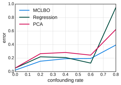
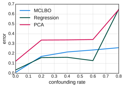
Figure 1: Simulation results for the correctly specified (left) and overspecified (right) confounder dimensionality. mcei performs similar or better than pca and better tolerates misspecification. Basic regression performs poorly at high levels of confounding.

Flexible Estimators.

With flexible estimators, there can be an issue that leads to high estimator variance. We illustrate this issue with the simple case of independent treatments. Suppose the true treatments ${\boldsymbol{\mathbf{t}}}_{j}$ come from an unconfounded model, where all of the ${\boldsymbol{\mathbf{t}}}_{j}$ are independent. Consider using a latent variable model for confounder estimation, where each observation has a latent variable ${\boldsymbol{\mathbf{z}}}$ and treatment vector ${\boldsymbol{\mathbf{t}}}$. Let $W$ be a matrix of parameters, let $\kappa$ and $\sigma$ be hyperparameters, and let $j$ index observations. Then the model is ${\boldsymbol{\mathbf{z}}}_{j}\sim\mathcal{N}(0,\sigma),\quad{\boldsymbol{\mathbf{t}}}_{j}\sim\mathcal{N}(W{\boldsymbol{\mathbf{z}}}_{j},\kappa)$. The maximum likelihood estimate for the this model with latent size equal to data size given this true model is $W^{*}=I(1-\kappa)$, up to rotations. Posterior distributions are a type of stochastic confounder estimator. Here, the posterior distribution is

$$p({\boldsymbol{\mathbf{z}}}\,|\,{\boldsymbol{\mathbf{t}}})=\mathcal{N}\left(\frac{\sigma}{\sigma+\kappa}{\boldsymbol{\mathbf{t}}},\sigma^{2}\left(1-\frac{\sigma}{\sigma+\kappa}\right)\right).$$

A range of estimators given by this posterior indexed by $\kappa$ have the same conditional entropy and predictive likelihoods. All residuals for any $\kappa>0$ recover the right causal effect. The trouble comes in as $\kappa$ gets small. Here the variance in the residual gets small, which in turn implies the variance of the estimated causal effect gets large similar to when using a weak instrument. In the appendix, we provide families of estimators that exhibit this problem for general treatments. If the estimator family is rich enough there may be multiple, ami regularization values $\alpha$ that lead to the same prediction. Choosing the largest value of ami regularization mitigates this issue by find the estimator in the equivalence class that leaves the most information for the residuals, thus reducing the variance of the causal estimates.

5 Experiments

We demonstrate our approach on a large simulation where the noise also grows with the amount of confounding. We study variants of the simulation where the estimators are misspecified. We also study a real-world example from medicine. Here, we look at the effects of various lab values prior to entering the intensive care unit on the length of stay in the hospital.

Simulation.

Consider a model with real-valued treatments. Let $n$ index the observations and $i$ the treatments. Let $W$ be a parameter matrix, $\sigma$ be the simulation standard deviation, $\gamma$ be the confounding rate, and $D$ be the dimensionality of ${\boldsymbol{\mathbf{z}}}$. The treatments are drawn conditional on an unobserved ${\boldsymbol{\mathbf{z}}}_{n}$ as

$${\boldsymbol{\mathbf{z}}}_{n}\sim\textrm{Normal} (0,\gamma),\quad{\boldsymbol{\mathbf{\epsilon}}}_{n}\sim\textrm{Normal}(0,1-\gamma),$$

$$t_{i,n}\sim\textrm{Normal}(W{\boldsymbol{\mathbf{z}}}+{\boldsymbol{\mathbf{\epsilon}}}_{n},\sigma),$$ (7)

where $\gamma$ scales the influence of ${\boldsymbol{\mathbf{z}}}_{n}$ on each of the treatments. Let $b$ be weight vectors and $\sigma_{y}$ be the outcome standard deviation. Then the outcomes are

$$y_{n}\sim\textrm{Normal}((1-\gamma)b_{\epsilon}^{\top}{\boldsymbol{\mathbf{\epsilon}}}_{n}+\gamma b_{{\boldsymbol{\mathbf{z}}}}^{\top}|{\boldsymbol{\mathbf{z}}}_{n}|,\sigma_{y}).$$

The amount of confounding grows with $\gamma$. The simulation is nonlinear and as the confounding rate grows, the estimation problem becomes harder because the $\sigma_{y}$ gets larger relative to the effects.

We compare our approach to the pca correction (Yu et al.,, 2006) which closely relates to lmm (Kang et al.,, 2010; Lippert et al.,, 2011). These approaches should perform well in confounding estimation since the process in eq. 7 matches the assumptions behind probabilistic pca (Bishop,, 2016). However because of the outcome information problem from the previous section, the results may be vary depending on whether the outcome model uses the estimated confounders. For confounder estimation by the mclbo, we limit mcei to have a similar number of parameters. Details are in the appendix.

We study two cases. First, we correctly give all methods the right dimensionality $D=2$. Second, we misspecify: all methods use a bigger dimension $10$, while the true $D=2$. We measure MSE to the true parameters scaled by the true norm. We simulate $10,000$ observations with $50$ treatments over $5$ redraws. We use neural networks for all functions and Gaussian likelihoods. We describe the remaining simulation parameters in the appendix.

Figure 1 shows the results. The left panel plots the error for varying levels of confounding when the confounder dimension is correctly specified. We find that confounder estimation with mcei performs similar to or better than pca. Regression performs poorly as the confounding grows. Though pca is the correct model to recover the unobserved confounders, the outcome model can ignore the confounder due to the information inequality in the previous section. The right panels show mcei tolerates misspecification better than pca.

Clinical Experiment.

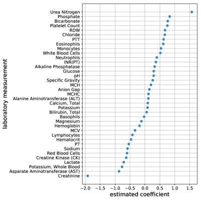
Figure 2: Causal estimates for effects of laboratory values on ICU length of stay.

Length of stay (los) is defined as the duration of a hospital visit. This measure is often used as an intermediate outcome in studies due to the associated adverse primary outcomes. Patient flow is important medically because unnecessarily prolonged hospitalization places patients at risk for hospital acquired infections (among other adverse outcomes). These can be difficult to treat and are associated with significant morbidity, mortality, and cost. Studies have found a 1.37% increase in infection risk and 6% increase in any adverse event risk for each excess los day (Hassan et al.,, 2010; Andrews et al.,, 1997). Also, it is of operational concern for hospitals because reimbursement for medical care is increasingly tied to visit episodes rather than to discrete products or services provided (Press et al.,, 2016).

The dataset studied in this experiment is comprised of 25753 ICU visits and 37 laboratory tests from the mimic iii clinical database (Johnson et al.,, 2016). We applied our mcei approach to laboratory tests measured in the emergency department prior to admission as treatments, and a binarized los based on the average value as outcome. Laboratory test values were shifted, log-transformed, and standardized with missing values imputed to the median of the laboratory test type.

The results are shown in fig. 2 and correlate well with findings in the literature regarding factors influencing los. For example, elevated blood urea nitrogen is associated with states of hypovolemia (prerenal azotemia) and hypercatabolism and has been linked to increased los in pancreatitis and stroke patients (Faisst et al.,, 2010; Lin et al.,, 2015). Elevated white blood cells, or leukocytosis, is one of the main markers for infection and, as expected, infection has been associated with increased los, particularly when systemic (Beyersmann et al.,, 2009; Talmor et al.,, 1999). Other findings, such as an inverse relationship to potassium (hypokalemia) is also supported by the literature (Paltiel et al.,, 2001). An inverse relationship with creatinine may be due to age, a confounder that was not included and likely violates the shared confounding because it primarily only effects creatinine.

6 Conclusion

We formalized two assumptions needed for multiple causal inference, namely shared confounding and independence between treatments given the shared confounders. Together, these assumptions imply a information-regularized estimator for unmeasured confounders. We developed lower bounds for a tractable algorithm. We showed how stochastic residuals can be used to estimate the outcome model, and we demonstrated our approach in simulations and on ICU data.

Many future directions remain. First, the assumptions we made are likely not tight. For example, the independence between treatments given the shared confounder could be relaxed to allow a finite number of dependencies between observations. The intuition is that if there is a limited amount of dependence between treatments, the confounder can be estimated from the other treatments. Next, in the algorithm to estimate the information, the lower bound can be replaced by likelihood ratio estimation. This has the benefit of removing slack in the bound, while also improving numerical stability by avoiding differences. Finally, with multiple outcomes, new kinds of estimators that are simpler can be developed.

Acknowledgments

We would like to acknowledge Jaan Altosaar, Fredrik Johansson, Rahul Krishnan, Aahlad Manas Puli, and Bharat Srikishan for helpful discussion and comments.

Appendix A Appendix

Big Estimator Classes.

Stochastic confounder estimators can be constructed by looking at posteriors of models. We construct a big estimator class by building two models that match the observed data and looking at mixtures of these two models. Both models have the same distribution of treatments and outcomes and have treatments that are independent of the outcome. Take the model

$${\boldsymbol{\mathbf{z}}} =f({\boldsymbol{\mathbf{\epsilon}}}_{\boldsymbol{\mathbf{z}}})$$

$$t_{i} =h_{i}({\boldsymbol{\mathbf{\epsilon}}}_{i},{\boldsymbol{\mathbf{z}}})$$

$$y =g({\boldsymbol{\mathbf{\epsilon}}}_{y},{\boldsymbol{\mathbf{z}}},t_{1},....t_{T}),$$

and the model

$${\boldsymbol{\mathbf{z}}} =f({\boldsymbol{\mathbf{\epsilon}}}_{\boldsymbol{\mathbf{z}}}),{\boldsymbol{\mathbf{\epsilon}}}_{1},...,{\boldsymbol{\mathbf{\epsilon}}}_{T}$$

$$t_{i} =h_{i}({\boldsymbol{\mathbf{z}}})$$

$$y =g({\boldsymbol{\mathbf{\epsilon}}}_{y},{\boldsymbol{\mathbf{z}}},h_{1}({\boldsymbol{\mathbf{z}}}),...,h_{T}({\boldsymbol{\mathbf{z}}})).$$

Both of these models satisfy the independence of treatments given the shared confounder and have the same joint distribution on ${\boldsymbol{\mathbf{t}}},y$. But the second model differs in key way. It assumes all of the treatments are due to confounding. Mixtures of these models also have the same distribution. As the mixing portion of the second model goes to one, the estimated causal effects would have high variance. Many ami regularization values have the same prediction error. To reduce variance, we select the largest ami regularization value in the class that predicts the best.

Negative Entropy Lower Bound

$$-\mathbb{H}_{\boldsymbol{\mathbf{\theta}}}({\boldsymbol{\mathbf{z}}}\,|\,{\boldsymbol{\mathbf{t}}}_{-i}) =\int p({\boldsymbol{\mathbf{z}}},{\boldsymbol{\mathbf{t}}}_{-i})\log p({\boldsymbol{\mathbf{z}}}\,|\,{\boldsymbol{\mathbf{t}}}_{-i})d{\boldsymbol{\mathbf{z}}}d{\boldsymbol{\mathbf{t}}}_{-i}$$

$$=\int p({\boldsymbol{\mathbf{z}}}\,|\,{\boldsymbol{\mathbf{t}}})p({\boldsymbol{\mathbf{t}}})\log p({\boldsymbol{\mathbf{z}}}\,|\,{\boldsymbol{\mathbf{t}}}_{-i})d{\boldsymbol{\mathbf{z}}}d{\boldsymbol{\mathbf{t}}}$$

$$=\int p({\boldsymbol{\mathbf{z}}}\,|\,{\boldsymbol{\mathbf{t}}})p({\boldsymbol{\mathbf{t}}})\log\left[\int p({\boldsymbol{\mathbf{z}}}\,|\,{\boldsymbol{\mathbf{t}}}_{-i},\hat{t}_{i})p(t_{i}=\hat{t}_{i}\,|\,{\boldsymbol{\mathbf{t}}}_{-i})d\hat{t}_{i}\right]d{\boldsymbol{\mathbf{z}}}d{\boldsymbol{\mathbf{t}}}$$

$$=\int p({\boldsymbol{\mathbf{z}}}\,|\,{\boldsymbol{\mathbf{t}}})p({\boldsymbol{\mathbf{t}}})\log\left[\int p({\boldsymbol{\mathbf{z}}}\,|\,{\boldsymbol{\mathbf{t}}}_{-i},\hat{t}_{i})\frac{p(t_{i}=\hat{t}_{i})p({\boldsymbol{\mathbf{t}}}_{-i}\,|\,t_{i}=\hat{t}_{i})}{p({\boldsymbol{\mathbf{t}}}_{-i})}d\hat{t}_{i}\right]d{\boldsymbol{\mathbf{z}}}d{\boldsymbol{\mathbf{t}}}$$

$$=\int p({\boldsymbol{\mathbf{z}}}\,|\,{\boldsymbol{\mathbf{t}}})p({\boldsymbol{\mathbf{t}}})\log\left[\int p(t_{i}=\hat{t}_{i})\frac{p({\boldsymbol{\mathbf{z}}}\,|\,{\boldsymbol{\mathbf{t}}}_{-i},\hat{t}_{i})p({\boldsymbol{\mathbf{t}}}_{-i}\,|\,t_{i}=\hat{t}_{i})}{p({\boldsymbol{\mathbf{t}}}_{-i})}d\hat{t}_{i}\right]d{\boldsymbol{\mathbf{z}}}d{\boldsymbol{\mathbf{t}}}$$

$$\geq\int p({\boldsymbol{\mathbf{z}}}\,|\,{\boldsymbol{\mathbf{t}}})p({\boldsymbol{\mathbf{t}}})\left[\int p(t_{i}=\hat{t}_{i})\log\frac{p({\boldsymbol{\mathbf{z}}}\,|\,{\boldsymbol{\mathbf{t}}}_{-i},\hat{t}_{i})p({\boldsymbol{\mathbf{t}}}_{-i}\,|\,t_{i}=\hat{t}_{i})}{p({\boldsymbol{\mathbf{t}}}_{-i})}d\hat{t}_{i}\right]d{\boldsymbol{\mathbf{z}}}d{\boldsymbol{\mathbf{t}}}$$

$$=\int p({\boldsymbol{\mathbf{z}}}\,|\,{\boldsymbol{\mathbf{t}}})p({\boldsymbol{\mathbf{t}}})p(t_{i}=\hat{t}_{i})\left(\log p({\boldsymbol{\mathbf{z}}}\,|\,{\boldsymbol{\mathbf{t}}}_{-i},\hat{t}_{i})+\log\frac{p({\boldsymbol{\mathbf{t}}}_{-i}\,|\,t_{i}=\hat{t}_{i})}{p({\boldsymbol{\mathbf{t}}}_{-i})}\right)d\hat{t}_{i}d{\boldsymbol{\mathbf{z}}}d{\boldsymbol{\mathbf{t}}}$$

$$=\int p({\boldsymbol{\mathbf{z}}}\,|\,{\boldsymbol{\mathbf{t}}})p({\boldsymbol{\mathbf{t}}})p(t_{i}=\hat{t}_{i})\log p({\boldsymbol{\mathbf{z}}}\,|\,{\boldsymbol{\mathbf{t}}}_{-i},\hat{t}_{i})d\hat{t}_{i}d{\boldsymbol{\mathbf{z}}}d{\boldsymbol{\mathbf{t}}}+\int p({\boldsymbol{\mathbf{z}}}\,|\,{\boldsymbol{\mathbf{t}}})p({\boldsymbol{\mathbf{t}}})p(t_{i}=\hat{t}_{i})\log\frac{p({\boldsymbol{\mathbf{t}}}_{-i}\,|\,t_{i}=\hat{t}_{i})}{p({\boldsymbol{\mathbf{t}}}_{-i})}d\hat{t}_{i}d{\boldsymbol{\mathbf{z}}}d{\boldsymbol{\mathbf{t}}}$$

$$=\int p({\boldsymbol{\mathbf{z}}}\,|\,{\boldsymbol{\mathbf{t}}})p({\boldsymbol{\mathbf{t}}})p(t_{i}=\hat{t}_{i})\log p({\boldsymbol{\mathbf{z}}}\,|\,{\boldsymbol{\mathbf{t}}}_{-i},\hat{t}_{i})d\hat{t}_{i}d{\boldsymbol{\mathbf{z}}}d{\boldsymbol{\mathbf{t}}}+C$$

The above bound does not require any extra parameters. It may however be loose. With an auxiliary parameter, we can create a bound that gets tighter as the auxiliary parameter is optimized. Let ${\boldsymbol{\mathbf{\xi}}}_{i}$ be an auxiliary parameter and $r$ a distribution parametrized by ${\boldsymbol{\mathbf{\xi}}}_{i}$, then we have the following lower bound on the negative mutual information

$$-\mathbb{I}(t_{i};{\boldsymbol{\mathbf{z}}}\,|\,{\boldsymbol{\mathbf{t}}}_{-i}) =-\textrm{KL}(p(t_{i};{\boldsymbol{\mathbf{z}}}\,|\,{\boldsymbol{\mathbf{t}}}_{-i})||p(t_{i}\,|\,{\boldsymbol{\mathbf{t}}}_{-i})p({\boldsymbol{\mathbf{z}}}\,|\,{\boldsymbol{\mathbf{t}}}_{-i}))=-\mathbb{E}_{p({\boldsymbol{\mathbf{t}}})p({\boldsymbol{\mathbf{z}}}\,|\,{\boldsymbol{\mathbf{t}}})}\log\frac{p(t_{i},{\boldsymbol{\mathbf{z}}}\,|\,{\boldsymbol{\mathbf{t}}}_{-i})}{p(t_{i}\,|\,{\boldsymbol{\mathbf{t}}}_{-i})p({\boldsymbol{\mathbf{z}}}\,|\,{\boldsymbol{\mathbf{t}}}_{-i})}$$

$$=-\left(\mathbb{E}_{p({\boldsymbol{\mathbf{t}}})p({\boldsymbol{\mathbf{z}}}\,|\,{\boldsymbol{\mathbf{t}}})}\log\frac{p(t_{i},{\boldsymbol{\mathbf{z}}}\,|\,{\boldsymbol{\mathbf{t}}}_{-i})}{p(t_{i}\,|\,{\boldsymbol{\mathbf{t}}}_{-i})p({\boldsymbol{\mathbf{z}}}\,|\,{\boldsymbol{\mathbf{t}}}_{-i})}+\mathbb{E}_{p({\boldsymbol{\mathbf{t}}}_{-i})}[\textrm{KL}(p({\boldsymbol{\mathbf{z}}}\,|\,{\boldsymbol{\mathbf{t}}}_{-i})||p({\boldsymbol{\mathbf{z}}}\,|\,{\boldsymbol{\mathbf{t}}}_{-i}))]\right)$$

$$\geq-\left(\mathbb{E}_{p({\boldsymbol{\mathbf{t}}})p({\boldsymbol{\mathbf{z}}}\,|\,{\boldsymbol{\mathbf{t}}})}\log\frac{p(t_{i},{\boldsymbol{\mathbf{z}}}\,|\,{\boldsymbol{\mathbf{t}}}_{-i})}{p(t_{i}\,|\,{\boldsymbol{\mathbf{t}}}_{-i})p({\boldsymbol{\mathbf{z}}}\,|\,{\boldsymbol{\mathbf{t}}}_{-i})}+\mathbb{E}_{p({\boldsymbol{\mathbf{t}}}_{-i})}[\textrm{KL}(p({\boldsymbol{\mathbf{z}}}\,|\,{\boldsymbol{\mathbf{t}}}_{-i})||r({\boldsymbol{\mathbf{z}}}\,|\,{\boldsymbol{\mathbf{t}}}_{-i};{\boldsymbol{\mathbf{\xi}}}_{i}))]\right)$$

$$=-\left(\mathbb{E}_{p({\boldsymbol{\mathbf{t}}})p({\boldsymbol{\mathbf{z}}}\,|\,{\boldsymbol{\mathbf{t}}})}\log\frac{p(t_{i},{\boldsymbol{\mathbf{z}}}\,|\,{\boldsymbol{\mathbf{t}}}_{-i})}{p(t_{i}\,|\,{\boldsymbol{\mathbf{t}}}_{-i})p({\boldsymbol{\mathbf{z}}}\,|\,{\boldsymbol{\mathbf{t}}}_{-i})}+\mathbb{E}_{p({\boldsymbol{\mathbf{t}}}_{-i})p({\boldsymbol{\mathbf{z}}}\,|\,{\boldsymbol{\mathbf{t}}}_{-i})}\log\frac{p({\boldsymbol{\mathbf{z}}}\,|\,{\boldsymbol{\mathbf{t}}}_{-i})}{r({\boldsymbol{\mathbf{z}}}\,|\,{\boldsymbol{\mathbf{t}}}_{-i};{\boldsymbol{\mathbf{\xi}}}_{i})}\right)$$

$$=-\left(\mathbb{E}_{p({\boldsymbol{\mathbf{t}}})p({\boldsymbol{\mathbf{z}}}\,|\,{\boldsymbol{\mathbf{t}}})}\log\frac{p(t_{i},{\boldsymbol{\mathbf{z}}}\,|\,{\boldsymbol{\mathbf{t}}}_{-i})}{p(t_{i}\,|\,{\boldsymbol{\mathbf{t}}}_{-i})p({\boldsymbol{\mathbf{z}}}\,|\,{\boldsymbol{\mathbf{t}}}_{-i})}+\mathbb{E}_{p({\boldsymbol{\mathbf{t}}})p({\boldsymbol{\mathbf{z}}}\,|\,{\boldsymbol{\mathbf{t}}})}\log\frac{p({\boldsymbol{\mathbf{z}}}\,|\,{\boldsymbol{\mathbf{t}}}_{-i})}{r({\boldsymbol{\mathbf{z}}}\,|\,{\boldsymbol{\mathbf{t}}}_{-i};{\boldsymbol{\mathbf{\xi}}}_{i})}\right)$$

$$=-\mathbb{E}_{p({\boldsymbol{\mathbf{t}}})p({\boldsymbol{\mathbf{z}}}\,|\,{\boldsymbol{\mathbf{t}}})}\log\frac{p(t_{i},{\boldsymbol{\mathbf{z}}}\,|\,{\boldsymbol{\mathbf{t}}}_{-i})}{p(t_{i}\,|\,{\boldsymbol{\mathbf{t}}}_{-i})r({\boldsymbol{\mathbf{z}}}\,|\,{\boldsymbol{\mathbf{t}}}_{-i};{\boldsymbol{\mathbf{\xi}}}_{i})}$$

$$=-\mathbb{E}_{p({\boldsymbol{\mathbf{t}}})p({\boldsymbol{\mathbf{z}}}\,|\,{\boldsymbol{\mathbf{t}}})}\log\frac{p({\boldsymbol{\mathbf{z}}}\,|\,{\boldsymbol{\mathbf{t}}})}{r({\boldsymbol{\mathbf{z}}}\,|\,{\boldsymbol{\mathbf{t}}}_{-i};{\boldsymbol{\mathbf{\xi}}}_{i})}$$

This is a lower bound because KL divergence is nonnegative. Maximizing this bound with respect to ${\boldsymbol{\mathbf{\xi}}}_{i}$ increases the tightness of the bound by minimizing the KL-divergence. The confounder parameters and the bound parameters can be simultaneously maximized. The bound is tight when $r({\boldsymbol{\mathbf{z}}}\,|\,{\boldsymbol{\mathbf{t}}}_{-i};{\boldsymbol{\mathbf{\xi}}}_{i})=p({\boldsymbol{\mathbf{z}}}\,|\,{\boldsymbol{\mathbf{t}}}_{-i})$, so if $r$ is rich enough to contain $p({\boldsymbol{\mathbf{z}}}\,|\,{\boldsymbol{\mathbf{t}}}_{-i})$. The gap will be zero. The introduction of the auxiliary distribution, $r$, is similar to those used in variational inference (Agakov and Barber,, 2004; Salimans et al.,, 2015; Ranganath et al.,, 2016; Maaløe et al.,, 2016).

Proposition 1.

Independence given the confounder means that $t_{i}$ is independent of $t_{j}$ given the unobserved confounder. Shared confounding means there is only a single confounder ${\boldsymbol{\mathbf{z}}}$. Since the form of $f$ is arbitrary, the distribution on ${\boldsymbol{\mathbf{z}}}$ is arbitrary. Also, since $h_{i}$ is arbitrary the distribution of $t_{j}$ given ${\boldsymbol{\mathbf{z}}}$ is arbitrary. Thus the generative process in Equation 1 constructs treatments that are conditionally independent given the confounder. It can represent any distribution for each treatment given the confounder. The confounder can also can take any distribution. This means that Equation 1 can represent any distribution of treatments that satisfy both assumptions, of shared confounding and of independence given confounding. The outcome function $g$ is arbitrary and so can be chosen to match any true outcome model.

Gradients of the mclbo.

The terms in the mclbo are all integrals with respect to the distribution $p_{\boldsymbol{\mathbf{\theta}}}({\boldsymbol{\mathbf{z}}}\,|\,{\boldsymbol{\mathbf{t}}})$. To compute stochastic gradients, we differentiate under the integral sign as in variational inference. For simplicity, we assume that a sample from $p_{\boldsymbol{\mathbf{\theta}}}({\boldsymbol{\mathbf{z}}}\,|\,{\boldsymbol{\mathbf{t}}})$ can be generated by transforming parameter-free noise ${\boldsymbol{\mathbf{\delta}}}\sim s$ through a function ${\boldsymbol{\mathbf{z}}}={\boldsymbol{\mathbf{z}}}({\boldsymbol{\mathbf{\delta}}},{\boldsymbol{\mathbf{\theta}}},{\boldsymbol{\mathbf{t}}})$. This assumption leads to simpler gradient computation (Kingma and Welling,, 2014; Rezende et al.,, 2014). The gradient with respect to ${\boldsymbol{\mathbf{\theta}}}$ can be written as

$$\nabla_{\boldsymbol{\mathbf{\theta}}}\mathcal{L}= \mathbb{E}_{p({\boldsymbol{\mathbf{t}}})}\mathbb{E}_{s({\boldsymbol{\mathbf{\delta}}})}\left[\nabla_{\boldsymbol{\mathbf{\theta}}}{\boldsymbol{\mathbf{z}}}({\boldsymbol{\mathbf{\delta}}},{\boldsymbol{\mathbf{\theta}}},{\boldsymbol{\mathbf{t}}})\nabla_{\boldsymbol{\mathbf{z}}}\sum_{i=1}^{T}\log p_{\boldsymbol{\mathbf{\beta}}}(t_{i}\,|\,{\boldsymbol{\mathbf{z}}})\right]$$

$$+\alpha\sum_{i=1}^{T}\mathbb{E}_{p({\boldsymbol{\mathbf{t}}})}\mathbb{E}_{s({\boldsymbol{\mathbf{\delta}}})}\left[\nabla_{\boldsymbol{\mathbf{\theta}}}{\boldsymbol{\mathbf{z}}}({\boldsymbol{\mathbf{\delta}}},{\boldsymbol{\mathbf{\theta}}},{\boldsymbol{\mathbf{t}}})\nabla_{\boldsymbol{\mathbf{z}}}\log r_{{\boldsymbol{\mathbf{\xi}}}_{i}}({\boldsymbol{\mathbf{z}}}\,|\,{\boldsymbol{\mathbf{t}}}_{-i})\right]$$

$$-\alpha T\mathbb{E}_{p({\boldsymbol{\mathbf{t}}})}\mathbb{E}_{s({\boldsymbol{\mathbf{\delta}}})}\left[\nabla_{\boldsymbol{\mathbf{\theta}}}{\boldsymbol{\mathbf{z}}}({\boldsymbol{\mathbf{\delta}}},{\boldsymbol{\mathbf{\theta}}},{\boldsymbol{\mathbf{t}}})\nabla_{\boldsymbol{\mathbf{z}}}\log p_{\boldsymbol{\mathbf{\theta}}}({\boldsymbol{\mathbf{z}}}\,|\,{\boldsymbol{\mathbf{t}}})\right].$$ (8)

Sampling from the various expectations gives a noisy unbiased estimate of the gradient. The gradient for ${\boldsymbol{\mathbf{\beta}}}$ is much simpler, as the sampled distributions do not depend on ${\boldsymbol{\mathbf{\beta}}}$:

$$\nabla_{\boldsymbol{\mathbf{\beta}}}\mathcal{L}=\mathbb{E}_{p({\boldsymbol{\mathbf{t}}})}\mathbb{E}_{p_{\boldsymbol{\mathbf{\theta}}}({\boldsymbol{\mathbf{z}}}\,|\,{\boldsymbol{\mathbf{t}}})}\left[\sum_{i=1}^{T}\nabla_{\boldsymbol{\mathbf{\beta}}}\log p_{\boldsymbol{\mathbf{\beta}}}({\boldsymbol{\mathbf{t}}}\,|\,{\boldsymbol{\mathbf{z}}})\right].$$ (9)

Sampling from the observed data then sampling the confounder estimate gives an unbiased estimate of this gradient. The gradient for ${\boldsymbol{\mathbf{\xi}}}_{i}$ follows similarly

$$\nabla_{\boldsymbol{\mathbf{\xi}}}\mathcal{L}=\alpha\mathbb{E}_{p({\boldsymbol{\mathbf{t}}})}\mathbb{E}_{p_{\boldsymbol{\mathbf{\theta}}}({\boldsymbol{\mathbf{z}}}\,|\,{\boldsymbol{\mathbf{t}}})}\left[\sum_{i=1}^{T}\nabla_{{\boldsymbol{\mathbf{\xi}}}_{i}}[\log r_{{\boldsymbol{\mathbf{\xi}}}_{i}}({\boldsymbol{\mathbf{z}}}\,|\,{\boldsymbol{\mathbf{t}}}_{-i})]\right]$$ (10)

The confounder estimation for a fixed value of $\alpha$ is summarized in Algorithm 1.

Equivalent Confounders.

Invertible transformations of a random variable preserve the information in that random variable. Take two distributions for computing the stochastic confounder ${\boldsymbol{\mathbf{z}}}_{1}\sim p_{1}(\cdot\,|\,{\boldsymbol{\mathbf{t}}})$ and ${\boldsymbol{\mathbf{z}}}_{2}\sim p_{2}(\cdot\,|\,{\boldsymbol{\mathbf{t}}})$ where ${\boldsymbol{\mathbf{z}}}_{2}$ can be written as an invertible function of ${\boldsymbol{\mathbf{z}}}_{1}$. These two distributions have equivalent information for downstream tasks, such as building the outcome model or conditioning on the confounder. This equivalence means we have choice on which member in the equivalence class we choose. One way to narrow the choice is to enforce that the dimensions of ${\boldsymbol{\mathbf{z}}}$ are independent by minimizing total correlation.

Connection to Factor Analysis.

Factor analysis methods work by specifying a generative model for observations that independently generate each dimension of each observation. In its most general form this model is

$${\boldsymbol{\mathbf{z}}}_{n}=f({\boldsymbol{\mathbf{\epsilon}}}_{z}),$$

$${\boldsymbol{\mathbf{t}}}_{n,i}=h_{i}({\boldsymbol{\mathbf{\epsilon}}}_{y},{\boldsymbol{\mathbf{z}}}_{n}).$$

Inference in this model matches the reconstruction term inside our confounder estimator with a $KL$-divergence regularizer. If we allow for the parameters of the prior on ${\boldsymbol{\mathbf{z}}}$ to be learned to maximize the overall likelihood, and if ${\boldsymbol{\mathbf{z}}}$’s dimensions are independent, then inference corresponds to minimizing the reconstruction eq. 2 with a total correlation style penalty.

There are many ways to choose the complexity of the factor model. One choice is to find the smallest complexity model that still gives good predictions of ${\boldsymbol{\mathbf{t}}}_{i}$ given ${\boldsymbol{\mathbf{t}}}_{-i}$ (like document completion evaluation in topic models (Wallach et al.,, 2009)). Here complexity is measured in terms of the dimensionality of ${\boldsymbol{\mathbf{z}}}$ and the complexity of $h_{i}$ and $f$. This choice tries to minimize the amount of information retained in ${\boldsymbol{\mathbf{z}}}$, while still reconstructing the treatments well. This way to select the factor analysis model’s complexity is a type of ami regularization. However, selecting discrete parameters like dimensionality give less fine-grained control over the information rates.

Proposition 2.

If the data are conditionally i.i.d., then in the true model ${\boldsymbol{\mathbf{z}}}$ concentrates as the number of treatments goes to infinity. In this setting, we can learn the model from Proposition 1 using the mclbo. This follows because the information each treatment provides goes to zero as $T\to\infty$ since they are conditionally i.i.d., thus the true confounder (and posterior), up to information equivalences, is simply a point that maximizes the reconstruction term in the mclbo subject to asymptotically zero ami. Identifying the parameters of the confounder estimator requires that $N\to\infty$. This shows outcome estimation corresponds to simple regression with treatments and confounder (up to an information equivalence), which correctly estimates the causal effects as $N\to\infty$.

Estimating ${\boldsymbol{\mathbf{\epsilon}}}_{i}$.

The ${\boldsymbol{\mathbf{\epsilon}}}_{i}$ estimation requires finding parameters ${\boldsymbol{\mathbf{\lambda}}}$ and ${\boldsymbol{\mathbf{\nu}}}$ that maximize

$$\mathbb{E}_{p({\boldsymbol{\mathbf{t}}})p_{\boldsymbol{\mathbf{\theta}}}({\boldsymbol{\mathbf{z}}}\,|\,{\boldsymbol{\mathbf{t}}})\prod_{i}p_{\boldsymbol{\mathbf{\lambda}}}({\boldsymbol{\mathbf{\epsilon}}}_{i}\,|\,{\boldsymbol{\mathbf{z}}},{\boldsymbol{\mathbf{t}}}_{i})}\left[\sum_{i=1}^{T}\log p_{\boldsymbol{\mathbf{\nu}}}(t_{i}\,|\,{\boldsymbol{\mathbf{z}}},{\boldsymbol{\mathbf{\epsilon}}}_{i})\right],\textrm{such that }\mathbb{I}[{\boldsymbol{\mathbf{\epsilon}}}_{i},{\boldsymbol{\mathbf{z}}}]=0.$$

The constraint can be baked into a Lagrangian with parameter $\kappa$,

$$\mathbb{E}_{p({\boldsymbol{\mathbf{t}}})p_{\boldsymbol{\mathbf{\theta}}}({\boldsymbol{\mathbf{z}}}\,|\,{\boldsymbol{\mathbf{t}}})\prod_{i}p_{\boldsymbol{\mathbf{\lambda}}}({\boldsymbol{\mathbf{\epsilon}}}_{i}\,|\,{\boldsymbol{\mathbf{z}}},{\boldsymbol{\mathbf{t}}}_{i})}\left[\sum_{i=1}^{T}\log p_{\boldsymbol{\mathbf{\nu}}}(t_{i}\,|\,{\boldsymbol{\mathbf{z}}},{\boldsymbol{\mathbf{\epsilon}}}_{i})\right]-\kappa\mathbb{I}[{\boldsymbol{\mathbf{\epsilon}}}_{i},{\boldsymbol{\mathbf{z}}}].$$

The mutual information can be split into entropy terms:

$$\mathbb{I}[{\boldsymbol{\mathbf{\epsilon}}}_{i},{\boldsymbol{\mathbf{z}}}]=\mathbb{H}({\boldsymbol{\mathbf{\epsilon}}}_{i})-\mathbb{H}({\boldsymbol{\mathbf{\epsilon}}}_{i}\,|\,{\boldsymbol{\mathbf{z}}}).$$

We can use the entropy bounds with auxiliary distributions on the conditioning set. These bounds work with a distribution over the reverse conditioning set in this case $r({\boldsymbol{\mathbf{t}}}\,|\,{\boldsymbol{\mathbf{z}}},{\boldsymbol{\mathbf{\epsilon}}}_{i})$. For this, we can use the reconstruction distribution $p_{\boldsymbol{\mathbf{\nu}}}(t_{i}\,|\,{\boldsymbol{\mathbf{z}}},{\boldsymbol{\mathbf{\epsilon}}}_{i})$ and the fact that $p({\boldsymbol{\mathbf{z}}})$ and $p({\boldsymbol{\mathbf{t}}})$ do not depend on the parameters ${\boldsymbol{\mathbf{\nu}}}$ and ${\boldsymbol{\mathbf{\theta}}}$.

Confounder Parameterization and Simulation Hyperparameters.

We limit the confounder to have similar complexity as pca. We do this by using a confounder distribution with normal noise, where we restrict the mean of the confounder estimate to be a linear function of the treatments ${\boldsymbol{\mathbf{t}}}$. The variance is independent and controlled by a two-layer (for second moments) neural network. We similarly limit the likelihoods and outcome model to have three-layer means and fixed variance.

For the remaining simulation hyperparameters, we set $W$ and $b$ to be the absolute value of draws from the standard normal. The weights $b_{\boldsymbol{\mathbf{\epsilon}}}$ is scaled by a decreasing sequence of $t^{-0.6}$ to ensure finite variance. We fix the simulation standard deviation to $0.02$ and fix outcome standard deviation to $0.1$.

References

- Agakov and Barber, (2004) Agakov, F. V. and Barber, D. (2004). An auxiliary variational method. In Neural Information Processing, pages 561–566.
- Andrews et al., (1997) Andrews, L. B., Stocking, C., Krizek, T., Gottlieb, L., Krizek, C., Vargish, T., and Siegler, M. (1997). An alternative strategy for studying adverse events in medical care. The Lancet, 349(9048):309–313.
- Angrist et al., (1996) Angrist, J. D., Imbens, G. W., and Rubin, D. B. (1996). Identification of causal effects using instrumental variables. Journal of the American statistical Association, 91(434):444–455.
- Beyersmann et al., (2009) Beyersmann, J., Kneib, T., Schumacher, M., and Gastmeier, P. (2009). Nosocomial infection, length of stay, and time-dependent bias. Infection Control & Hospital Epidemiology, 30(3):273–276.
- Bishop, (2016) Bishop, C. (2016). Pattern Recognition and Machine Learning. Springer-Verlag New York.
- Consortium et al., (2007) Consortium, W. T. C. C. et al. (2007). Genome-wide association study of 14,000 cases of seven common diseases and 3,000 shared controls. Nature, 447(7145):661.
- Cook et al., (2002) Cook, T. D., Campbell, D. T., and Shadish, W. (2002). Experimental and quasi-experimental designs for generalized causal inference. Houghton Mifflin Boston.
- Cover and Thomas, (2012) Cover, T. M. and Thomas, J. A. (2012). Elements of information theory. John Wiley & Sons.
- D’Amour, (2018) D’Amour, A. (2018). (Non-)identification in latent confounder models. http://www.alexdamour.com/blog/public/2018/05/18/non-identification-in-latent-confounder-models/.
- Faisst et al., (2010) Faisst, M., Wellner, U. F., Utzolino, S., Hopt, U. T., and Keck, T. (2010). Elevated blood urea nitrogen is an independent risk factor of prolonged intensive care unit stay due to acute necrotizing pancreatitis. Journal of critical care, 25(1):105–111.
- Hassan et al., (2010) Hassan, M., Tuckman, H. P., Patrick, R. H., Kountz, D. S., and Kohn, J. L. (2010). Hospital length of stay and probability of acquiring infection. International Journal of pharmaceutical and healthcare marketing, 4(4):324–338.
- Hill, (2011) Hill, J. L. (2011). Bayesian nonparametric modeling for causal inference. Journal of Computational and Graphical Statistics, 20(1):217–240.
- Hoyer et al., (2009) Hoyer, P. O., Janzing, D., Mooij, J. M., Peters, J., and Schölkopf, B. (2009). Nonlinear causal discovery with additive noise models. In Advances in neural information processing systems, pages 689–696.
- Johansson et al., (2016) Johansson, F., Shalit, U., and Sontag, D. (2016). Learning representations for counterfactual inference. In International Conference on Machine Learning, pages 3020–3029.
- Johnson et al., (2016) Johnson, A. E., Pollard, T. J., Shen, L., Li-wei, H. L., Feng, M., Ghassemi, M., Moody, B., Szolovits, P., Celi, L. A., and Mark, R. G. (2016). Mimic-iii, a freely accessible critical care database. Scientific data, 3:160035.
- Kang et al., (2010) Kang, H. M., Sul, J. H., Zaitlen, N. A., Kong, S.-y., Freimer, N. B., Sabatti, C., Eskin, E., et al. (2010). Variance component model to account for sample structure in genome-wide association studies. Nature genetics, 42(4):348.
- Kingma and Welling, (2014) Kingma, D. and Welling, M. (2014). Auto-encoding variational bayes. In International Conference on Learning Representations (ICLR-14).
- Kocaoglu et al., (2017) Kocaoglu, M., Snyder, C., Dimakis, A. G., and Vishwanath, S. (2017). Causalgan: Learning causal implicit generative models with adversarial training. arXiv preprint arXiv:1709.02023.
- Lin et al., (2015) Lin, W.-C., Shih, H.-M., and Lin, L.-C. (2015). Preliminary prospective study to assess the effect of early blood urea nitrogen/creatinine ratio-based hydration therapy on poststroke infection rate and length of stay in acute ischemic stroke. Journal of Stroke and Cerebrovascular Diseases, 24(12):2720–2727.
- Lippert et al., (2011) Lippert, C., Listgarten, J., Liu, Y., Kadie, C. M., Davidson, R. I., and Heckerman, D. (2011). Fast linear mixed models for genome-wide association studies. Nature methods, 8(10):833.
- Louizos et al., (2017) Louizos, C., Shalit, U., Mooij, J. M., Sontag, D., Zemel, R., and Welling, M. (2017). Causal effect inference with deep latent-variable models. In Advances in Neural Information Processing Systems, pages 6449–6459.
- Maaløe et al., (2016) Maaløe, L., Sønderby, C. K., Sønderby, S. K., and Winther, O. (2016). Auxiliary deep generative models. arXiv preprint arXiv:1602.05473.
- Morgan and Winship, (2014) Morgan, S. L. and Winship, C. (2014). Counterfactuals and causal inference. Cambridge University Press.
- O’connor et al., (2009) O’connor, C., Adhikari, N. K., DeCaire, K., and Friedrich, J. O. (2009). Medical admission order sets to improve deep vein thrombosis prophylaxis rates and other outcomes. Journal of hospital medicine, 4(2):81–89.
- Paltiel et al., (2001) Paltiel, O., Salakhov, E., Ronen, I., Berg, D., and Israeli, A. (2001). Management of severe hypokalemia in hospitalized patients: a study of quality of care based on computerized databases. Archives of internal medicine, 161(8):1089–1095.
- Pearl et al., (2009) Pearl, J. et al. (2009). Causal inference in statistics: An overview. Statistics surveys, 3:96–146.
- Press et al., (2016) Press, M. J., Rajkumar, R., and Conway, P. H. (2016). Medicare’s new bundled payments: design, strategy, and evolution. Jama, 315(2):131–132.
- Ranganath et al., (2014) Ranganath, R., Gerrish, S., and Blei, D. (2014). Black box variational inference. In Artificial Intelligence and Statistics, pages 814–822.
- Ranganath et al., (2016) Ranganath, R., Tran, D., and Blei, D. (2016). Hierarchical variational models. In International Conference on Machine Learning, pages 324–333.
- Rezende et al., (2014) Rezende, D. J., Mohamed, S., and Wierstra, D. (2014). Stochastic backpropagation and approximate inference in deep generative models. In International Conference on Machine Learning, pages 1278–1286.
- Rosenbaum and Rubin, (1983) Rosenbaum, P. R. and Rubin, D. B. (1983). The central role of the propensity score in observational studies for causal effects. Biometrika, 70(1):41–55.
- Salimans et al., (2015) Salimans, T., Kingma, D., and Welling, M. (2015). Markov chain monte carlo and variational inference: Bridging the gap. In International Conference on Machine Learning, pages 1218–1226.
- Shalit et al., (2017) Shalit, U., Johansson, F. D., and Sontag, D. (2017). Estimating individual treatment effect: generalization bounds and algorithms. In International Conference on Machine Learning, pages 3076–3085.
- Song et al., (2015) Song, M., Hao, W., and Storey, J. D. (2015). Testing for genetic associations in arbitrarily structured populations. Nature genetics, 47(5):550.
- Talmor et al., (1999) Talmor, M., Hydo, L., and Barie, P. S. (1999). Relationship of systemic inflammatory response syndrome to organ dysfunction, length of stay, and mortality in critical surgical illness: effect of intensive care unit resuscitation. Archives of surgery, 134(1):81–87.
- Tran and Blei, (2017) Tran, D. and Blei, D. M. (2017). Implicit causal models for genome-wide association studies. arXiv preprint arXiv:1710.10742.
- Wager and Athey, (2017) Wager, S. and Athey, S. (2017). Estimation and inference of heterogeneous treatment effects using random forests. Journal of the American Statistical Association, (just-accepted).
- Wallach et al., (2009) Wallach, H. M., Murray, I., Salakhutdinov, R., and Mimno, D. (2009). Evaluation methods for topic models. In Proceedings of the 26th annual international conference on machine learning, pages 1105–1112. ACM.
- Wang and Blei, (2018) Wang, Y. and Blei, D. M. (2018). The blessings of multiple causes. arXiv preprint arXiv:1805.06826.
- Williams, (1992) Williams, R. J. (1992). Simple statistical gradient-following algorithms for connectionist reinforcement learning. In Reinforcement Learning, pages 5–32. Springer.
- Yu et al., (2006) Yu, J., Pressoir, G., Briggs, W. H., Bi, I. V., Yamasaki, M., Doebley, J. F., McMullen, M. D., Gaut, B. S., Nielsen, D. M., Holland, J. B., et al. (2006). A unified mixed-model method for association mapping that accounts for multiple levels of relatedness. Nature genetics, 38(2):203.