“Direct” Gas-Phase Metallicity in Local Analogs of High-Redshift Galaxies: Empirical Metallicity Calibrations for High-Redshift Star-Forming Galaxies

Abstract

We study the direct gas-phase oxygen abundance using the well-detected auroral line [O III]$\lambda$4363 in the stacked spectra of a sample of local analogs of high-redshift galaxies. These local analogs share the same location as $z\sim 2$ star-forming galaxies on the [O III]$\lambda$5007/H$\beta$ versus [N II]$\lambda$6584/H$\alpha$ Baldwin-Phillips-Terlevich diagram. This type of analog has the same ionized interstellar medium (ISM) properties as high-redshift galaxies. We establish empirical metallicity calibrations between the direct gas-phase oxygen abundances ($7.8<12+\log(\rm{O/H})<8.4$) and the N2 ($\log$([N II]$\lambda$6584/H$\alpha$))/O3N2 ($\log$(([O III]$\lambda\lambda$4959,5007/H$\beta$)/([N II]$\lambda$6584/H$\alpha$))) indices in our local analogs. We find significant systematic offsets between the metallicity calibrations for our local analogs of high-redshift galaxies and those derived from the local H II regions and a sample of local reference galaxies selected from the Sloan Digital Sky Survey (SDSS). The N2 and O3N2 metallicities will be underestimated by 0.05-0.1 dex relative to our calibration, if one simply applies the local metallicity calibration in previous studies to high-redshift galaxies. Local metallicity calibrations also cause discrepancies of metallicity measurements in high-redshift galaxies using the N2 and O3N2 indicators. In contrast, our new calibrations produce consistent metallicities between these two indicators. We also derive metallicity calibrations for R23 ($\log$(([O III]$\lambda\lambda$4959,5007+[O II]$\lambda\lambda$3726,3729)/H$\beta$)), O32($\log$([O III]$\lambda\lambda$4959,5007/[O II]$\lambda\lambda$3726,3729)), $\log($[O III]$\lambda$5007/H$\beta$), and $\log$([Ne III]$\lambda$3869/[O II]$\lambda$3727) indices in our local analogs, which show significant offset compared to those in the SDSS reference galaxies. By comparing with MAPPINGS photoionization models, the different empirical metallicity calibration relations in the local analogs and the SDSS reference galaxies can be shown to be primarily due to the change of ionized ISM conditions. Assuming that temperature structure variations are minimal and ISM conditions do not change dramatically from $z\sim 2$ to $z\sim 5$, these empirical calibrations can be used to measure relative metallicities in galaxies with the redshifts up to $z\sim 5.0$ in ground-based observations.

1 Introduction

Studies of galaxy chemical abundances across cosmic history provide insight into the key physical processes governing the formation and evolution of galaxies (e.g., Finlator & Davé, 2008; Davé et al., 2012; Lilly et al., 2013; Lu et al., 2015; Ma et al., 2016). A relationship between galaxy stellar mass and gas-phase oxygen abundance has been well established in the local universe (Tremonti et al., 2004; Savaglio et al., 2005; Kewley & Ellison, 2008; Andrews & Martini, 2013). Galaxies with higher stellar masses tend to have higher metallicities than galaxies with lower stellar masses. An evolution of the mass-metallicity relation has been found in galaxies up to a redshift of $z\sim 3.5$ (Erb et al., 2006; Maiolino et al., 2008; Zahid et al., 2013, 2014; Maier et al., 2014; Steidel et al., 2014; Sanders et al., 2015; Guo et al., 2016; Ly et al., 2016b; Onodera et al., 2016). High-redshift star-forming galaxies have lower metallicities for a given stellar mass compared to galaxies at lower redshift.

There are three ways to measure the gas-phase oxygen abundances:

1. Theoretical metallicity calibrations, which combine stellar synthesis models (e.g., Starburst99, Leitherer et al., 1999) and photoionization models, including MAPPINGS (Sutherland & Dopita, 1993; Dopita et al., 2013) and CLOUDY (Ferland et al., 2013), to predict the metallicity-sensitive emission-line ratios based on input metallicities (e.g., McGaugh, 1991; Kewley & Dopita, 2002; Tremonti et al., 2004; Dopita et al., 2016).

2. The $``T_{e}"$ or “direct” method, which measures electron temperature using the ratio of the [O III]$\lambda$4363 auroral emission line to the [O III]$\lambda$5007 emission line. This method requires one to correct for unseen stages of ionization and assume a uniform electron temperature throughout the gas. The metallicity is then estimated based on the electron temperature (e.g., Pagel et al., 1992; Izotov et al., 2006).

3. Empirical metallicity calibrations, which establish relations between the $T_{e}$ metallicity and the strong line ratios to overcome the difficulty of detecting the weak [O III]$\lambda$4363 auroral emission line (e.g., Pettini & Pagel, 2004; Pilyugin & Thuan, 2005; Nagao et al., 2006; Pilyugin et al., 2010, 2012; Pérez-Montero & Contini, 2009; Marino et al., 2013; Brown et al., 2016; Cowie et al., 2016; Curti et al., 2017). For example, Pettini & Pagel (2004, PP04 hereafter) fit the relationship between the direct $T_{e}$-based metallicities and strong emission-line ratios, including the $N2=\log$([N II]$\lambda$6584/H$\alpha$) and $O3N2=\log$[([O III]$\lambda$5007/H$\beta$)/([N II]$\lambda$6584/H$\alpha$)] indices in a sample of H II regions in nearby star-forming galaxies. These empirical calibrations based on local H II regions have been widely used to estimate the metallicities in high-redshift galaxies (e.g., Erb et al., 2006; Hainline et al., 2009; Bian et al., 2010; Steidel et al., 2014; Sanders et al., 2015), though it is unclear whether these empirical calibrations are still feasible for high-redshift star-forming galaxies.

Photoionization models show that the [N II]$\lambda$6584/H$\alpha$ and [O III]$\lambda$5007/H$\beta$ ratios depend not only on the metallicity but also on other effects, including the ionization parameter, the electron density, the nitrogen-to-oxygen ratio (N/O), and the spectral shape of the radiation field (e.g., Kewley & Dopita, 2002; Kewley et al., 2013a, b; Cullen et al., 2016; Hirschmann et al., 2017). If one or a combination of these factors changes with cosmic time, metallicity calibrations derived from local galaxies will not be applicable to high-redshift galaxies (e.g., Bian et al., 2017). Changes in the physical conditions of the ionized ISM condition and/or the radiation field can also shift the location of high-redshift galaxies in the [O III]$\lambda$5007/H$\beta$ versus [N II]$\lambda$6584/H$\alpha$ “Baldwin-Phillips-Terlevich” (BPT, Baldwin et al., 1981; Veilleux & Osterbrock, 1987) diagram and in other commonly used diagnostic diagrams (e.g., Figure 1, Kewley et al., 2013a, b, 2016; Steidel et al., 2014; Shapley et al., 2015; Sanders et al., 2016b; Bian et al., 2016). Using these diagrams, studies have shown that the ionization parameter, electron density (e.g., Brinchmann et al., 2008; Liu et al., 2008; Kewley et al., 2013a, b; Nakajima & Ouchi, 2014; Shirazi et al., 2014; Sanders et al., 2016b; Kaasinen et al., 2017), hardness of the stellar radiation fields (e.g., Steidel et al., 2014; Strom et al., 2017b, a), and/or the relation between N/O and metallicity (e.g., Masters et al., 2014; Shapley et al., 2015) might change across cosmic time. These potential changes raise a crucial question: are the empirical calibrations based on the local H II regions still valid for high-redshift galaxies?

There are two methods by which to resolve this issue:

1. Implementing the effects of changing ISM conditions, radiation field, and N/O within photoionization models to obtain metallicity diagnostics for high-redshift galaxies that explicitly take these changes into account. Unfortunately for this approach, there exist degeneracies when using the BPT and other optical diagnostic diagrams to study how the above effects vary with redshift. It is still under debate which one or a combination of the above effects change with redshift and by how much.

2. Establishing the empirical relation between direct $``T_{e}"$ metallicity and the strong emission line in high-redshift galaxies. The “direct” gas-phase oxygen abundance has been well measured up to the redshift of $z\simeq 1.0$ (e.g., Ly et al., 2014, 2015, 2016a, 2016b; Jones et al., 2015). However, the [O III]$\lambda$4363 emission line is rarely detected in high-redshift galaxies at $z\sim 2$ (e.g., Yuan & Kewley, 2009; Rigby et al., 2011; Christensen et al., 2012; Sanders et al., 2016a). Alternatively, the O III]$\lambda\lambda$1661,1666 inter-combination emission line also can be used to measure the direct metallicity, however, the sample size is still small (e.g., James et al., 2014; Steidel et al., 2014, 2016; Kojima et al., 2016; Vanzella et al., 2016).

In this paper, we use a sample of local analogs of high-redshift galaxies selected from the Sloan Digital Sky Survey (SDSS) to study the empirical calibration at $z\sim 2$. These local analogs share the same region on the BPT diagram with $z\sim 2$ star-forming galaxies from Steidel et al. (2014). Bian et al. (2016) demonstrated that the galaxies with this BPT location selection have the same ionized ISM properties of $z\sim 2$ galaxies. Here, we use the stacked spectrum of both our analogs and the SDSS reference galaxies to detect the weak [O III]$\lambda$4363 line and measure the direct $T_{e}$ metallicity, which enables us to compare how the empirical metallicity calibration changes with redshift. This paper is organized as follows. In Section 2, we select an SDSS reference galaxy sample and a sample of local analogs of high-redshift galaxies. In Section 3, we measure the direct $T_{e}$ oxygen abundance in the stacked spectra of the SDSS reference galaxy sample and the local analog galaxy sample in different $N2$ bins. In Section 4, we establish the relation between the direct $T_{e}$ oxygen abundance and the metallicity diagnostic line ratios to study how the changes in the ISM conditions affect these empirical metallicity calibrations. In Section 5, we compare our new empirical metallicity calibrations with other empirical calibrations and photoionization models. In Section 6, we summarize the main results of this paper.

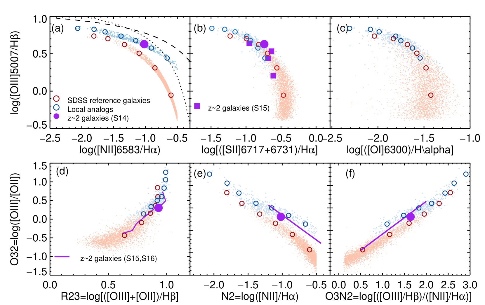
Figure 1: Diagnostic diagrams of local analogs of high-redshift galaxies and SDSS reference galaxies. The small blue and red points represent the individual local analogs and SDSS reference galaxies, respectively, and the large open blue and red points represent the stacked spectra of the local analogs and SDSS reference galaxies, respectively. The large purple filled circle represents the stacked spectrum of a sample of $z\sim 2$ UV-selected galaxies adopted from Steidel et al. (2014, S14). The purple squares represent the median distribution of a sample of $z\sim 2$ mass-selected galaxies adopted from Shapley et al. (2015, S15), and the purple solid lines represent the median distribution of a sample of $z\sim 2$ mass-selected galaxies adopted from Shapley et al. (2015, S15) and Sanders et al. (2016b, S16). The dotted and dashed lines in panel (a) represent the empirical (Kauffmann et al., 2003b) and theoretical (Kewley et al., 2001) separations of star-forming galaxies and AGNs, respectively.

2 Sample Selection

In this section, we select a sample of local reference galaxies and local analogs of high-redshift galaxies from the SDSS (York et al., 2000) MPA-JHU value-added catalog for SDSS Data Release 7 (Abazajian et al., 2009). The MPA-JHU catalog includes 819,333 galaxies, which are the part of the SDSS “main” galaxy sample (Strauss et al., 2002). The MPA-JHU catalog contains information on the fluxes, equivalent widths, and line widths of the optical emission lines, including [O II]$\lambda 3727$, H$\beta$, [O III]$\lambda\lambda 4959,5007$, H$\alpha$, [NII]$\lambda 6583$, and [S II]$\lambda\lambda 6717,6731$, stellar masses ($M_{*}$, Kauffmann et al., 2003a), star formation rates (SFRs, Brinchmann et al., 2004), and specific SFRs (SFR/$M_{*}$, sSFRs, Brinchmann et al., 2004). We first select galaxies that were classified as star-forming or starburst in the MPA-JHU catalog. Then we require the signal-to-noise ratios (S/Ns) of [O II]$\lambda$3727, H$\beta$, [O III]$\lambda\lambda 4959,5007$, H$\alpha$ and [N II]$\lambda$6583 emission lines greater than 10 in the MPA-JHU catalog. At last, we select the local reference galaxies and local analogs based on their locations on the BPT diagram.

2.1 SDSS Reference Galaxy Sample

We select local reference galaxies located in the $\pm 0.05$ dex region of the local star-forming sequence defined by the equation 3 in Kewley et al. (2013a) on the BPT diagram as follows (red small data points in Figure 1(a)):

$$\log({\rm[OIII]/H\beta)})>\frac{0.61}{\log({\rm[NII]/H\alpha)})-0.08}+1.05,$$ (1)

$$\log({\rm[OIII]/H\beta)})<\frac{0.61}{\log({\rm[NII]/H\alpha)}-0.08}+1.15,$$ (2)

and

$$\log({\rm[NII]/H\alpha)}<-0.5$$ (3)

The following [S II]$\lambda\lambda 6717,6731$ and [O I]$\lambda$6300 diagnostics are applied to further remove galaxies with AGN/shock contamination to the emission-line flux (Kewley et al., 2006)

$$\log({\rm[OIII]/H\beta})<\frac{0.72}{\log({\rm[SII]/H\alpha})-0.32}+1.30$$ (4)

$$\log({\rm[OIII]/H\beta})<\frac{0.73}{\log({\rm[OI]/H\alpha})-0.59}+1.33$$ (5)

A total of 22428 unique SDSS galaxies are selected. In general, these galaxies represent low-redshift star-forming galaxies, which are located on the local BPT star-forming sequence.

2.2 Local Analogs of High-redshift Galaxies

The sample of local analogs of high-redshift galaxies has been selected from in the $\pm 0.04$ dex region of the $z\sim 2.3$ star-forming sequence defined by equation 9 in Steidel et al. (2014) on the BPT diagram (blue small data points in Figure 1(a)):

$$\log({\rm[OIII]/H\beta)})>\frac{0.67}{\log({\rm[NII]/H\alpha)})-0.33}+1.09,$$ (6)

$$\log({\rm[OIII]/H\beta)})<\frac{0.67}{\log({\rm[NII]/H\alpha)})-0.33}+1.17,$$ (7)

and

$$\log({\rm[NII]/H\alpha)})<-0.5$$ (8)

All the galaxies selected by equations of 6 - 8 are classified as galaxies by the Kewley et al. (2001) criterion (Figure 1(a)), and all the galaxies with $\log$([N II]$\lambda$6584/H$\alpha$$)<-0.75$ are classified as galaxies by the Kauffmann et al. (2003b) criterion. We further apply the [S II] and [O I] BPT diagnostic to reduce the AGN/shock contaminants. Studies have shown that $z\sim 2$ star-forming galaxies exhibit a higher [O III]/H$\beta$ ratio for a given [S II]/H$\alpha$ ratio (e.g., Strom et al., 2017b). Thus, we shift the Kewley et al. (2006) criteria on the [O III]/H$\beta$ ratio by +0.05 dex for high-redshift galaxies.

$$\log({\rm[OIII]/H\beta})<\frac{0.72}{\log({\rm[SII]/H\alpha})-0.32}+1.35$$ (9)

$$\log({\rm[OIII]/H\beta})<\frac{0.73}{\log({\rm[OI]/H\alpha})-0.59}+1.38$$ (10)

A total of 443 galaxies are selected based on the above selection criteria. Equations 9 and 10 remove about 20%, and these two criteria do not affect the distribution of the local analogs on the optical diagnostics diagrams. We cross-correlate the positions of the analogs of high-redshift galaxies with the ROSAT ALL-Sky Survey Faint Source Catalog (Voges et al., 2000) and find that none of the analogs are detected at X-ray wavelengths. We further check the local analogs with high-redshift galaxies with high full width half maximum of the Balmer emission lines to remove potential AGNs hosting low-mass supermassive black holes ($10^{6}~{}M_{\sun}$ with $\rm FWHM>600$ km s^-1, Greene & Ho, 2004). We find only one galaxy with $\rm FWHM>400$ km s^-1 among our local analogs, and the galaxy is removed from our further analysis. We also visually inspect the image of the local analogs and their fiber positions to remove spurious galaxies being targeted due to poor photometric deblending. The properties of these local analogs can be summarized as follows. The median stellar mass is $\log(M_{*}/M_{\sun})=8.8\begin{subarray}{c}+0.06\\ -0.02\end{subarray}$. The median SFR and sSFR are $3.9\begin{subarray}{c}+0.7\\ -0.2\end{subarray}$ $M_{\sun}$ yr^-1 and $10.0\begin{subarray}{c}+1.0\\ -0.5\end{subarray}$ Gyr^-1, respectively. The sSFR of the local analogs is comparable to that in $z\sim 2$ star-forming galaxies with similar stellar mass (e.g., Rodighiero et al., 2011). Furthermore, these analogs closely resemble the ISM conditions in high-redshift galaxies, including high ionization parameters ($\log q\simeq 7.9$ cm^-1) and high electron densities ($n_{e}\simeq 120$ cm^-3). The median ionization parameters and electron densities in these analogs are also comparable to those in the $z\sim 2-3$ galaxies (e.g., Nakajima & Ouchi, 2014; Sanders et al., 2016b). We refer readers to Bian et al. (2016, 2017) for more details.

Table 1: The Relative Line Flux from the Stacked Spectra of the SDSS Reference Galaxies

line	N2${}_{-0.75}^{-0.50}$	N2${}_{-1.00}^{-0.75}$	N2${}_{-1.25}^{-1.00}$	N2${}_{-1.50}^{-1.25}$	N2${}_{-1.75}^{-1.50}$	N2${}_{-2.00}^{-1.75}$	N2${}_{-2.25}^{-2.00}$
[O II]$\lambda 3727$	$3.301\pm 0.038$	$3.513\pm 0.023$	$3.088\pm 0.014$	$2.523\pm 0.011$	$1.750\pm 0.009$	$1.071\pm 0.007$	$0.566\pm 0.011$
[Ne III]$\lambda 3869$	$0.125\pm 0.008$	$0.198\pm 0.007$	$0.287\pm 0.007$	$0.368\pm 0.009$	$0.427\pm 0.008$	$0.451\pm 0.007$	$0.512\pm 0.010$
[O III]$\lambda 4363$	$0.006\pm 0.004$	$0.015\pm 0.002$	$0.027\pm 0.001$	$0.045\pm 0.001$	$0.077\pm 0.001$	$0.116\pm 0.001$	$0.156\pm 0.002$
H$\beta$	$1.000\pm 0.073$	$1.000\pm 0.073$	$1.000\pm 0.080$	$1.000\pm 0.102$	$1.000\pm 0.235$	$1.000\pm 0.383$	$1.000\pm 0.865$
[O III]$\lambda 4959$	$0.290\pm 0.003$	$0.679\pm 0.003$	$1.069\pm 0.003$	$1.407\pm 0.003$	$1.672\pm 0.006$	$1.824\pm 0.008$	$2.198\pm 0.011$
[O III]$\lambda 5007$	$0.878\pm 0.007$	$2.038\pm 0.009$	$3.199\pm 0.009$	$4.190\pm 0.010$	$5.022\pm 0.017$	$5.453\pm 0.022$	$6.660\pm 0.033$
[O I]$\lambda 6100$	$0.107\pm 0.002$	$0.095\pm 0.001$	$0.076\pm 0.000$	$0.060\pm 0.000$	$0.042\pm 0.001$	$0.026\pm 0.001$	$0.014\pm 0.001$
[N II]$\lambda 6548$	$0.233\pm 0.002$	$0.130\pm 0.001$	$0.073\pm 0.000$	$0.043\pm 0.001$	$0.023\pm 0.001$	$0.014\pm 0.001$	$0.010\pm 0.001$
H$\alpha$	$2.860\pm 0.016$	$2.860\pm 0.009$	$2.860\pm 0.006$	$2.860\pm 0.005$	$2.860\pm 0.007$	$2.860\pm 0.009$	$2.860\pm 0.010$
[N II]$\lambda 6584$	$0.720\pm 0.004$	$0.402\pm 0.001$	$0.228\pm 0.001$	$0.134\pm 0.001$	$0.074\pm 0.001$	$0.044\pm 0.001$	$0.026\pm 0.001$
[S II]$\lambda 6717$	$0.529\pm 0.001$	$0.421\pm 0.000$	$0.311\pm 0.000$	$0.233\pm 0.000$	$0.155\pm 0.001$	$0.094\pm 0.001$	$0.051\pm 0.001$
[S II]$\lambda 6731$	$0.372\pm 0.001$	$0.299\pm 0.000$	$0.222\pm 0.000$	$0.166\pm 0.000$	$0.111\pm 0.001$	$0.069\pm 0.001$	$0.040\pm 0.001$
used	n	n	y	y	y	y	n
$T_{e}$ Metallicity	-	-	$8.26\pm 0.02$	$8.18\pm 0.009$	$8.00\pm 0.008$	$7.80\pm 0.006$	-

Table 2: The Relative Line Flux in the Spectra of the Local Analogs of High-redshift Galaxies.

line	N${}_{-0.75}^{-0.50}$	N${}_{-1.00}^{-0.75}$	N${}_{-1.25}^{-1.00}$	N${}_{-1.50}^{-1.25}$	N${}_{-1.75}^{-1.50}$	N${}_{-2.00}^{-1.75}$	N${}_{-2.25}^{-2.00}$
[O II]$\lambda 3727$	$2.757\pm 0.030$	$2.404\pm 0.023$	$2.071\pm 0.011$	$1.881\pm 0.008$	$1.264\pm 0.005$	$0.819\pm 0.012$	$0.532\pm 0.007$
[Ne III]$\lambda 3869$	$0.245\pm 0.010$	$0.313\pm 0.008$	$0.400\pm 0.007$	$0.464\pm 0.008$	$0.514\pm 0.007$	$0.514\pm 0.007$	$0.537\pm 0.010$
[O III]$\lambda 4363$	$0.017\pm 0.003$	$0.024\pm 0.001$	$0.043\pm 0.001$	$0.063\pm 0.001$	$0.095\pm 0.001$	$0.132\pm 0.001$	$0.167\pm 0.002$
H$\beta$	$1.000\pm 0.007$	$1.000\pm 0.007$	$1.000\pm 0.004$	$1.000\pm 0.003$	$1.000\pm 0.003$	$1.000\pm 0.005$	$1.000\pm 0.007$
[O III]$\lambda 4959$	$0.899\pm 0.007$	$1.244\pm 0.009$	$1.563\pm 0.006$	$1.797\pm 0.005$	$2.059\pm 0.006$	$2.251\pm 0.011$	$2.348\pm 0.016$
[O III]$\lambda 5007$	$2.761\pm 0.019$	$3.761\pm 0.025$	$4.713\pm 0.018$	$5.427\pm 0.015$	$6.196\pm 0.016$	$6.705\pm 0.031$	$6.912\pm 0.047$
[O I]$\lambda 6100$	$0.082\pm 0.001$	$0.068\pm 0.002$	$0.051\pm 0.001$	$0.045\pm 0.001$	$0.030\pm 0.000$	$0.024\pm 0.001$	$0.014\pm 0.001$
[N II]$\lambda 6548$	$0.208\pm 0.002$	$0.109\pm 0.001$	$0.063\pm 0.001$	$0.034\pm 0.001$	$0.022\pm 0.001$	$0.014\pm 0.001$	$0.010\pm 0.001$
H$\alpha$	$2.860\pm 0.015$	$2.860\pm 0.014$	$2.860\pm 0.008$	$2.860\pm 0.006$	$2.860\pm 0.006$	$2.860\pm 0.010$	$2.860\pm 0.014$
[N II]$\lambda 6584$	$0.626\pm 0.004$	$0.354\pm 0.002$	$0.201\pm 0.001$	$0.118\pm 0.001$	$0.066\pm 0.001$	$0.045\pm 0.001$	$0.025\pm 0.001$
[S II]$\lambda 6717$	$0.269\pm 0.002$	$0.220\pm 0.002$	$0.174\pm 0.001$	$0.153\pm 0.001$	$0.104\pm 0.001$	$0.076\pm 0.001$	$0.050\pm 0.001$
[S II]$\lambda 6731$	$0.223\pm 0.002$	$0.172\pm 0.002$	$0.132\pm 0.001$	$0.116\pm 0.001$	$0.080\pm 0.001$	$0.057\pm 0.001$	$0.037\pm 0.001$
used	n	y	y	y	y	y	y
$T_{e}$ Metallicity	-	$8.37\pm 0.02$	$8.25\pm 0.01$	$8.16\pm 0.009$	$8.03\pm 0.006$	$7.91\pm 0.006$	$7.81\pm 0.008$

2.3 Diagnostic Diagrams

Figure 1(a) shows the selection of the analogs of high-redshift galaxies and normal SDSS galaxies in the reference sample in the [O III]$\lambda$5007/H$\beta$ versus [N II]$\lambda$6584/H$\alpha$ BPT diagram. In addition, we compare the location of our local analogs and normal SDSS galaxies in other optical diagnostic diagrams in Figure 1(b-e). We find that our analogs share the same regions with $z\sim 2$ star-forming galaxies in all these diagnostic diagrams (Steidel et al., 2014; Shapley et al., 2015; Sanders et al., 2016b). Compared to normal SDSS galaxies, our analogs do not show offsets in the [O III]$\lambda$5007/H$\beta$ vs. [S II]$\lambda\lambda$6717,6731/H$\alpha$ (S2-) BPT diagram (Figure 1(b)) and O32 vs. R23 diagram (Figure 1(d)), but do show shifts in the O32 vs. N2 and O32 vs. O3N2 diagrams (Figures 1(e) and 1(f)). We also find no significant offset between our analogs and local SDSS galaxies in the [O III]$\lambda$5007/H$\beta$ vs. [O I]$\lambda$6300/H$\alpha$ (O1-) BPT diagram (Figure 1(c)). The O1-BPT diagram has not been studied in $z\sim 2$ galaxies, and our result can be tested in the future studies of $z\sim 2$ galaxies.

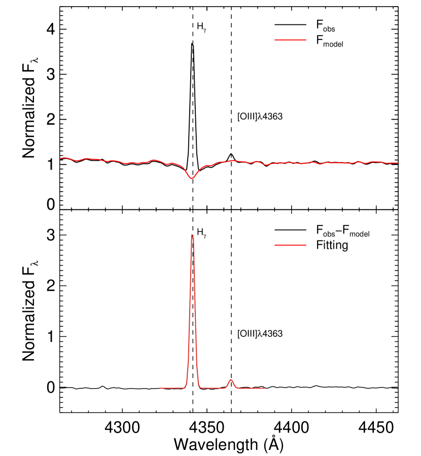
Figure 2: Example of stacked spectra and the stellar continuum and emission line fitting in the wavelength range close to H$\gamma$ and [O III]$\lambda$4363. Top panel: The black solid line represents an example of the stacked spectrum and the red line represents the best-fit stellar continuum for the stacked spectrum. Bottom panel: The black solid line represents the stellar-continuum subtracted spectrum and the red line represents the fitting result of H$\gamma$ and [O III]$\lambda$4363 emission line.

3 Analysis

3.1 Generating Stacked Spectra

We cannot detect the weak [O III]$\lambda$4363 emission line in most of our individual spectra. To increase the signal-to-noise ratio, we combine the spectra and generate stacked spectra for both our local analogs and selected SDSS galaxies. We adopt the procedure that has been used in Andrews & Martini (2013) and Brown et al. (2016), except we carry out dust extinction correction before stacking the spectra. The procedure is as follows:

1. We obtain the reduced one-dimensional SDSS spectra from the SDSS DR9 data release. The spectra were taken using the multi-object, fiber-fed spectrographs (Smee et al., 2013) mounted on the 2.5m telescope of SDSS (Gunn et al., 2006). The spectra have been reduced by the SDSS spectro2d pipeline (Stoughton et al., 2002).

2. Each of the SDSS galaxy spectra is corrected for the dust extinction using the Balmer decrement (H$\alpha$/H$\beta$) assuming Case B recombination and the Cardelli et al. (1989) dust extinction law.

3. Each SDSS spectrum is shifted to the rest frame based on the redshift from the MPA/JHU catalog.

4. Each of the SDSS spectra is resampled onto a wavelength grid in the $3700-7300$Å range with $\Delta\lambda=1$Å while maintaining flux conservation.

5. We normalize the spectra with the mean flux density in the $4400-4450$Å wavelength range.

6. We divide the local analogs and the selected SDSS galaxies separately into 0.25 dex bins in [N II]$\lambda$6584/H$\alpha$ from $\log$([N II]$\lambda$6584/H$\alpha$)$=x$ to $x+0.25$, where $x=[-2.25,-2.00,-1.75,-1.50,-1.25,-1.00,-0.75]$. We use the N2${}^{x+0.25}_{x}$ to represent the $\log$([N II]$\lambda$6584/H$\alpha$) between $x$ and $x+0.25$ for the remainder of the paper.

7. We stack the spectra falling into each of the [N II]$\lambda$6584/H$\alpha$ bins using the mean flux density at each wavelength.

Following the above procedure, we generate a total of 14 stacked spectra: 7 for the local analogs of high-redshift galaxies and 7 for the SDSS reference sample.

3.2 Subtracting the Stellar Component

The underlying stellar absorption features in the stacked spectra affect the emission-line flux measurements. In particular, the H$\gamma$ stellar absorption feature is close to the [O III]$\lambda$4363 emission line. Therefore, to measure the line fluxes accurately, it is important to subtract the stellar continuum from the stacked spectra. We fit the stellar continuum of each stacked spectrum with a set of stellar synthesis models using the STARLIGHT stellar population synthesis code (Cid Fernandes et al., 2005). We mask out the emission-line region before fitting the spectra. The Bruzual & Charlot (2003) stellar synthesis models with a Chabrier initial mass function (Chabrier, 2003) are adopted to fit the stacked spectra. These stellar synthesis models cover a broad range of metallicity ($0.05Z_{\sun}-2.5Z_{\sun}$) and stellar age ($1~{}\rm{Myr}-13$ Gyr). The upper panel of Figure 2 shows an example of the observed stacked spectrum ($F_{\rm obs}$) and the model spectrum ($F_{\rm model}$) from the best-fit stellar synthesis model at the wavelength close to the H$\gamma$ and [O III$]\lambda$4363 lines. The model spectrum follows the continuum of the observed spectrum and captures most of the spectral absorption features, suggesting our stellar synthesis model fitting process is robust.

3.3 Measuring Emission Line Flux

We measure the following emission-line fluxes in the stellar continuum subtracted stacked spectra: [O II]$\lambda\lambda$3726,3729, H$\gamma$, [O III]$\lambda$4363, H$\beta$, H$\alpha$, [N II]$\lambda\lambda$6548,6584, and [S II]$\lambda\lambda$6717,6731. We use the IDL MPFIT package to fit the emission lines by assuming that the emission-line profile follows the Gaussian distribution. A single Gaussian function is used to fit the emission lines that are well separated ($>30$ Å) from other emission lines, including the H$\beta$, [O III]$\lambda$4959, [O III]$\lambda$5007. Two Gaussians are fit simultaneously to those pairs of lines closer than 30 Å, including the H$\gamma$ and [O III]$\lambda$4363 pair, the [O II]$\lambda\lambda$3726,3729 doublet, and the [S II]$\lambda\lambda$6717,6731 doublet. As for the H$\alpha$ and [N II]$\lambda\lambda$6548,6584 complex, three Gaussians are used to fit simultaneously. In the fitting process, the central wavelength is fixed to the vacuum wavelength of the emission lines. We adopt the standard deviation of the continuum region close to ($<100$ Å) the emission-line-fitting regions as the 1$\sigma$ noise of the spectra. We carry out Monte Carlo simulations to estimate the uncertainties of line fluxes. A thousand simulated spectra are generated. The flux densities of these simulated spectra at each wavelength follow a Gaussian distribution whose center is at the actual flux density, and the standard derivation is consistent with 1$\sigma$ error at that wavelength. The bottom panel of Figure 2 shows the model-subtracted spectrum ($F_{\rm obs}-F_{\rm model}$) and best Gaussian fit for the H$\gamma$ and [O III]$\lambda$4363 line, which demonstrates that our line-fitting is robust. Tables 1 and 2 summarize the emission-line fluxes in each stacked spectrum.

Figure 1(a) shows the location of the stacked spectrum on the [O III]$\lambda$5007/H$\beta$ versus the [N II]$\lambda$6584/H$\alpha$ BPT diagram. We find that all the stacked spectra closely trace the local star-forming sequence and high-redshift star-forming sequence on the BPT diagram except the stacked spectrum of normal SDSS galaxies in the N2${}^{-2.25}_{-2.00}$ bin. However, only two galaxies in the SDSS reference galaxy sample fall into the N2${}^{-2.25}_{-2.00}$ bin, and both of them are located above the local star-forming sequence, biasing the stack spectrum toward the high-redshift star-forming sequence. Therefore, this data point is discarded for further analysis.

To achieve reliable direct oxygen abundance measurements, we only use the stacked spectra with S/Ns [O III]$\lambda$4363 greater than ten ($\rm S/N>10$) for further analysis.

3.4 Measuring the Direct Oxygen Abundance

We adopt the Izotov et al. (2006) recipe to derive the direct $T_{e}$ oxygen abundance. This method builds up a relation between the [O III]$\lambda\lambda$4959,5007/[O III]$\lambda$4363 ratio and the electron temperature in the O⁺⁺ zone ($T_{e}$(O III)). This relation also weakly depends on the electron density, which can be estimated from the [S II]$\lambda\lambda$6717,6731 doublet ratio. We do not have directly measured electron temperatures in the O⁺ zone ($T_{e}$(O II)). We adopt a relation between $T_{e}$(O III) and $T_{e}$(O II) from Garnett (1992) and Campbell et al. (1986) as follow: $T_{e}$(O II)=0.7$T_{e}$(O III)+3000K. We estimate the O⁺⁺ abundance using the $T_{e}$(O III) temperature and [O III]$\lambda\lambda$4959,5007/H$\beta$ ratio and O⁺ abundance using the $T_{e}$(O II) temperature, [O II]$\lambda\lambda$3726,3729/H$\beta$ and electron density. We compute the oxygen abundance by summing the O⁺⁺ abundance and the O⁺ abundance. We refer the reader to section 3.1 in Izotov et al. (2006) for more details.

3.5 Interstellar Medium Conditions

We study the ISM conditions, including the ionization parameter and electron density in the SDSS reference galaxies and local analogs of high-redshift galaxies. We estimate the ionization parameter in stacked spectrum in each N2 bin by adopting the recipe that first introduced in Kobulnicky & Kewley (2004) (see also Kewley & Ellison, 2008). This method is based on the Kewley & Dopita (2002) photoionization models. The ionization parameter is calculated by primarily using the O32. For a fixed O32, the oxygen abundance has a secondary effect on the ionization parameter measurement. So we further correct for the ionization parameter based on the oxygen abundance from the R23 and N2O2. We refer readers to section A2.3 in Kewley & Ellison (2008) for more details on the ionization parameter measurements. We estimate the electron density in each of the stacked spectra based on the [S II]$\lambda$6717/[S II]$\lambda$6731 ratio by adopting the nebular.temden routine in IRAF(Shaw & Dufour, 1995). Tables 4 and 4 summarize the results of the ionization parameters and electron densities in the SDSS reference galaxies and local analogs. We also list the median stellar mass and SFR for each N2 bin in Tables 4 and 4. The stellar masses of the local analogs and SDSS reference galaxies are consistent with each other in each of the N2 bins. The local analogs have higher ionization parameters ($\sim 0.3$ dex), higher SFRs, and higher electron densities (a factor of $\sim 5$) than SDSS reference galaxies in all N2 bins except the N${}_{-2.00}^{-2.25}$ bin, suggesting that the ISM conditions change significantly between the SDSS reference galaxies and local analogs.

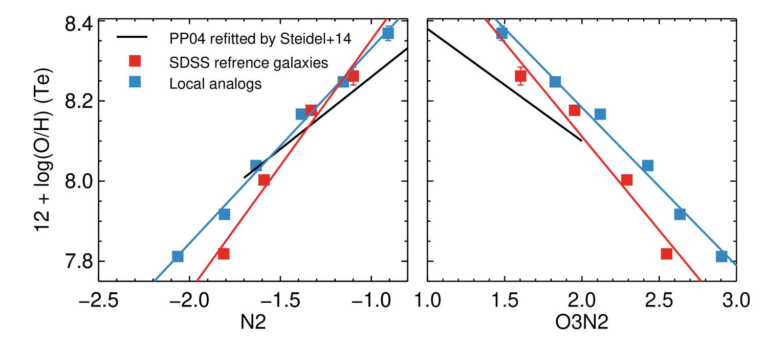
Figure 3: Relations between the direct oxygen abundance and N2 (left) and O3N2 (right) indices in the local analogs of high-redshift galaxies and the SDSS reference galaxies. The blue and red filled squares represent the local analogs and the SDSS reference galaxies, respectively. The blue and red lines represent the best fit of the relations between the direct oxygen abundance and N2 and O3N2 indices for the local analogs and the SDSS reference galaxies, respectively. The black line represents the empirical relation between the oxygen abundance and N2 and O3N2 indices from Steidel et al. (2014), who refitted the N2 and O3N2 metallicity calibrations of PP04 in the range of $-1.7<\rm{N2}<-0.3$ and $-0.4<\rm{O3N2}<2.1$

Table 3: The Properties of the SDSS Reference Galaxies.

Bin	#	SFR	Stellar Mass	$\log q$	$n_{e}$	$T_{e}$ Metallicity
		$M_{\sun}$ yr-1	$\log(M_{*}/M_{\sun})$	cm s-1	cm-3	$12+\log(\rm{O/H})$
N2${}_{-0.75}^{-0.50}$	15927	$1.1\begin{subarray}{c}+1.7\\ -0.7\end{subarray}$	$9.6\begin{subarray}{c}+0.3\\ -0.3\end{subarray}$	$7.39\pm 0.02$	$5\begin{subarray}{c}+9\\ -2\end{subarray}$	-
N2${}_{-1.00}^{-0.75}$	4491	$0.9\begin{subarray}{c}+2.2\\ -0.6\end{subarray}$	$9.2\begin{subarray}{c}+0.3\\ -0.3\end{subarray}$	$7.57\pm 0.03$	$16\begin{subarray}{c}+18\\ -14\end{subarray}$	-
N2${}_{-1.25}^{-1.00}$	1595	$0.7\begin{subarray}{c}+1.9\\ -0.5\end{subarray}$	$8.9\begin{subarray}{c}+0.4\\ -0.5\end{subarray}$	$7.72\pm 0.04$	$22\begin{subarray}{c}+25\\ -19\end{subarray}$	$8.26\pm 0.02$
N2${}_{-1.50}^{-1.25}$	333	$0.5\begin{subarray}{c}+1.2\\ -0.3\end{subarray}$	$8.3\begin{subarray}{c}+0.5\\ -0.5\end{subarray}$	$7.74\pm 0.03$	$21\begin{subarray}{c}+25\\ -17\end{subarray}$	$8.18\pm 0.009$
N2${}_{-1.75}^{-1.50}$	63	$0.5\begin{subarray}{c}+1.6\\ -0.3\end{subarray}$	$7.8\begin{subarray}{c}+0.5\\ -0.4\end{subarray}$	$7.92\pm 0.07$	$34\begin{subarray}{c}+42\\ -25\end{subarray}$	$8.00\pm 0.008$
N2${}_{-2.00}^{-1.75}$	17	$0.5\begin{subarray}{c}+0.9\\ -0.2\end{subarray}$	$7.7\begin{subarray}{c}+0.2\\ -0.5\end{subarray}$	$8.10\pm 0.11$	$51\begin{subarray}{c}+72\\ -31\end{subarray}$	$7.80\pm 0.006$
N2${}_{-2.25}^{-2.00}$	2	$0.6\begin{subarray}{c}+1.5\\ -0.2\end{subarray}$	$7.3\begin{subarray}{c}+0.4\\ -0.4\end{subarray}$	$8.44\pm 0.15$	$167\begin{subarray}{c}+204\\ -132\end{subarray}$	-

Table 4: The properties of the local analogs of high-redshift galaxies.

Bin	#	SFR	Stellar Mass	$\log q$	$n_{e}$
		$M_{\sun}$ yr-1	$\log(M_{*}/M_{\sun})$	cm s-1	cm-3	$12+\log(\rm{O/H})$
N2${}_{-0.75}^{-0.50}$	45	$3.4\begin{subarray}{c}+12.3\\ -2.9\end{subarray}$	$9.6\begin{subarray}{c}+0.3\\ -0.7\end{subarray}$	$7.77\pm 0.09$	$255\begin{subarray}{c}+277\\ -235\end{subarray}$	-
N2${}_{-1.00}^{-0.75}$	69	$13.5\begin{subarray}{c}+20.3\\ -11.2\end{subarray}$	$9.2\begin{subarray}{c}+0.3\\ -0.3\end{subarray}$	$7.88\pm 0.18$	$159\begin{subarray}{c}+177\\ -141\end{subarray}$	$8.37\pm 0.02$
N2${}_{-1.25}^{-1.00}$	110	$8.0\begin{subarray}{c}+20.3\\ -6.5\end{subarray}$	$8.9\begin{subarray}{c}+0.4\\ -0.6\end{subarray}$	$7.97\pm 0.16$	$110\begin{subarray}{c}+119\\ -102\end{subarray}$	$8.25\pm 0.01$
N2${}_{-1.50}^{-1.25}$	99	$2.6\begin{subarray}{c}+6.6\\ -2.0\end{subarray}$	$8.4\begin{subarray}{c}+0.4\\ -0.5\end{subarray}$	$7.95\pm 0.08$	$111\begin{subarray}{c}+124\\ -98\end{subarray}$	$8.16\pm 0.009$
N2${}_{-1.75}^{-1.50}$	44	$1.2\begin{subarray}{c}+1.7\\ -0.8\end{subarray}$	$8.0\begin{subarray}{c}+0.3\\ -0.3\end{subarray}$	$8.14\pm 0.10$	$132\begin{subarray}{c}+156\\ -109\end{subarray}$	$8.03\pm 0.006$
N2${}_{-2.00}^{-1.75}$	11	$1.8\begin{subarray}{c}+2.1\\ -1.7\end{subarray}$	$7.8\begin{subarray}{c}+0.2\\ -0.4\end{subarray}$	$8.33\pm 0.14$	$95\begin{subarray}{c}+137\\ -56\end{subarray}$	$7.91\pm 0.006$
N2${}_{-2.25}^{-2.00}$	2	$0.4\begin{subarray}{c}+1.7\\ -0.2\end{subarray}$	$7.3\begin{subarray}{c}+0.4\\ -0.1\end{subarray}$	$8.50\pm 0.14$	$97\begin{subarray}{c}+144\\ -54\end{subarray}$	$7.81\pm 0.008$

4 Results

4.1 N2 and O3N2 Empirical Metallicity Calibrations

Here, we investigate the N2 and O3N2 empirical metallicity calibrations in the local analogs and the SDSS reference galaxies by using the direct oxygen abundance and line ratios measured in the stacked spectrum. Figure 3 shows the relation between the direct $T_{e}$ oxygen abundance and the N2 and O3N2 indices in the local analogs of high-redshift galaxies (blue squares) and the local normal star-forming galaxies (red squares). The relation between the direct oxygen abundance and the N2 and O3N2 indices is fit with a linear equation for both the local analogs of high-redshift galaxies and SDSS reference galaxies. The results for the least-squares fit for our local analogs as follows (blue solid lines in Figure 3):

$$12+\log(\rm{{O}/{H}})=8.82+0.49\times\rm{N2},$$ (11)

$$12+\log(\rm{{O}/{H}})=8.97-0.39\times\rm{O3N2},$$ (12)

The results for the SDSS reference galaxies are as follows (red solid lines in Figure 3):

$$12+\log(\rm{{O}/{H}})=8.98+0.63\times\rm{N2},$$ (13)

$$12+\log(\rm{{O}/{H}})=9.05-0.47\times\rm{O3N2},$$ (14)

where $7.8<12+\log(\rm{{O}/{H}})<8.4$

In Figure 3, we compare our N2 and O3N2 calibrations in the local analogs, the SDSS reference galaxies, and the local H II regions. For the local H II region, we use the metallicity calibrations from Steidel et al. (2014) rather than those from PP04. Steidel et al. (2014) repeated the fits to N2 and O3N2 metallicity calibrations in PP04, but only focused on the H II regions with direct $T_{e}$ metallicity and in the low-metallicity range ($-1.7<\rm{N2}<-0.3$ and $-0.4<\rm{O3N2}<2.1$). Thus, the metallicity calibrations from Steidel et al. (2014) provide better comparisons with the relations in this work. The new N2 and O3N2 calibrations based on the local analogs are not consistent with those found in both the SDSS reference galaxies and the local H II region PP04. The discrepancies between the SDSS reference galaxies and the local H II regions are mainly caused by the contribution of diffused ionized gas emission in the SDSS reference galaxies (Sanders et al., 2017) and slightly different recipes for deriving the direct $T_{e}$ metallicity. The contribution of the diffused ionized gas emission in the local analogs is negligible due to their high H$\alpha$ surface density (Zhang et al., 2017). The direct $T_{e}$-based metallicity in the local analogs is systematically higher than that in the SDSS reference galaxies for a given N2 or O3N2 in the metallicity range of $7.8<12+\log(\rm O/\rm H)<8.4$. This discrepancy is mainly due to the changes of ISM conditions between our analogs and normal SDSS star-forming galaxies. The high ionization parameter and electron density increase the [N II]$\lambda$6584 and [O III]$\lambda$5007 line fluxes for a given metallicity, which causes the lower N2 and higher O3N2 values in the analogs (Dopita et al., 2016, see Section 5.3 for a further discussion).

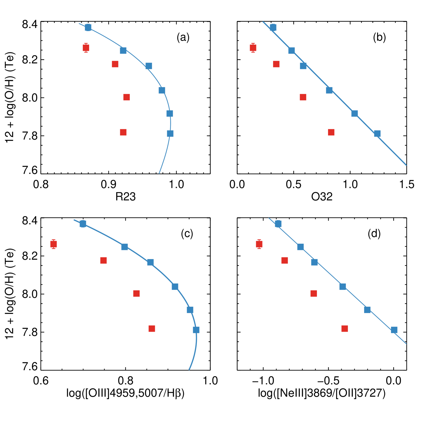
Figure 4: Relation between the direct oxygen abundance and R23, O32, $\log$[O III]$\lambda\lambda$4959,5007/H$\beta$, and $\log$([Ne III]$\lambda$3869/[O II]$\lambda$3727) indices. The blue filled squares represent the local analogs of high-redshift galaxies, and the red filled squares represent the SDSS reference galaxies.

4.2 Empirical Metallicity Calibrations for R23, O32, [O III]$\lambda\lambda$4959,5007/H$\beta$, and [Ne III]/[O II]

The H$\alpha$ and [N II]$\lambda$6584 emission lines move out of the $K$-band atmospheric transmission window for galaxies at $z>2.65$. Therefore, metallicity diagnostics based on the emission lines at shorter wavelengths are essential for galaxies at $z>2.65$. We study the empirical metallicity calibrations for the R23, O32 and [O III]$\lambda\lambda$4959,5007/H$\beta$, and [Ne III]$\lambda$3869/[O II] ratios. The [O II], [O III], H$\beta$, [Ne III] lines can be accessed in the $H$- and $K$-bands for galaxies at $z\sim 3.5$, and the [Ne III]/[O II] ratio can be measured in galaxies with redshift as high as $z=5.0$. These lines provide a powerful tool to measure the metallicity in galaxies at high redshift by assuming the ISM conditions did not change dramatically from $z=2$ to $z=5$.

Figure 4 shows the relation between the $T_{e}$ metallicity and the four metallicity diagnostics measured previously. We find that the our local analogs and normal SDSS galaxies do not follow the same relation in all four relations. For a given metallicity, the R23, O32, [O III]$\lambda\lambda$4959,5007/H$\beta$, and [Ne III]/[O II] ratios in the local analogs are higher that those in the normal SDSS galaxies. We fit the relations between the metallicity and R23, O32, [O III]$\lambda\lambda$4959,5007/H$\beta$, and [Ne III]/[O II] ratios for the local analogs of high-redshift galaxies. These relations are suitable for the metallicity range of $7.8<12+\log(\rm O/\rm H)<8.4$.

For the R23-Z relation, our data only cover the R23 upper branch and the transition zone of the R23 upper and lower branches. We fit the upper branch of the R23-Z relation using a third-order polynomial:

$$y=138.0430-54.8284x+7.2954x^{2}-0.32293x^{3}$$ (15)

where $y=R23$ and $x=12+\log(\rm{O/H})$. It is worth noting that the metallicity is not very sensitive to the R23 values in the metallicity range of $7.8<12+\log(\rm O/\rm H)<8.4$, because most of the data points are located in the transition zone of the R23 upper and lower branches.

For the O32-Z relation, we fit the data points using a linear equation:

$$12+\log(\rm{{O}/{H}})=8.54-0.59\times\rm{O32}.$$ (16)

For the [O III]$\lambda\lambda$4959,5007/H$\beta$-Z relation, we fit the data points using a third-order polynomial:

$$y=43.9836-21.6211x+3.4277x^{2}-0.1747x^{3}$$ (17)

where $y=$[O III]$\lambda\lambda$4959,5007/H$\beta$ and $x=12+\log(\rm{O/H})$.

For the [NeIII]/[OII]-Z relation, we fit the data points using a linear equation:

$$12+\log(\rm{{O}/{H}})=7.80-0.63\times\rm{\log([NeIII]/[OII])}.$$ (18)

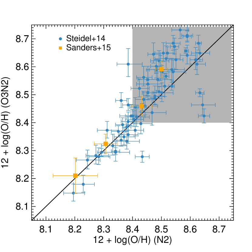
Figure 5: Comparison between the N2-based metallicity and O3N2-based metallicity in $z\sim 2$ star-forming galaxies using the BKD18 (this work) calibrations in this study. The blue filled circles represent the individual spectra of $z\sim 2$ UV-selected star-forming galaxies from Steidel et al. (2014, S14). The orange filled circles represent the stacked spectra of $z\sim 2$ mass-selected star-forming galaxies in four mass bins from Sanders et al. (2015, S15). The shaded region denotes the metallicity range in which the BKD18 calibrations are not valid. The BKD18 calibrations are valid in the metallicity range $7.8<12+\log(\rm O/\rm H)<8.4$. In this metallicity range, the N2- and O3N2-based metallicity are consistent with each other in both UV-selected and mass-selected star-forming galaxies.

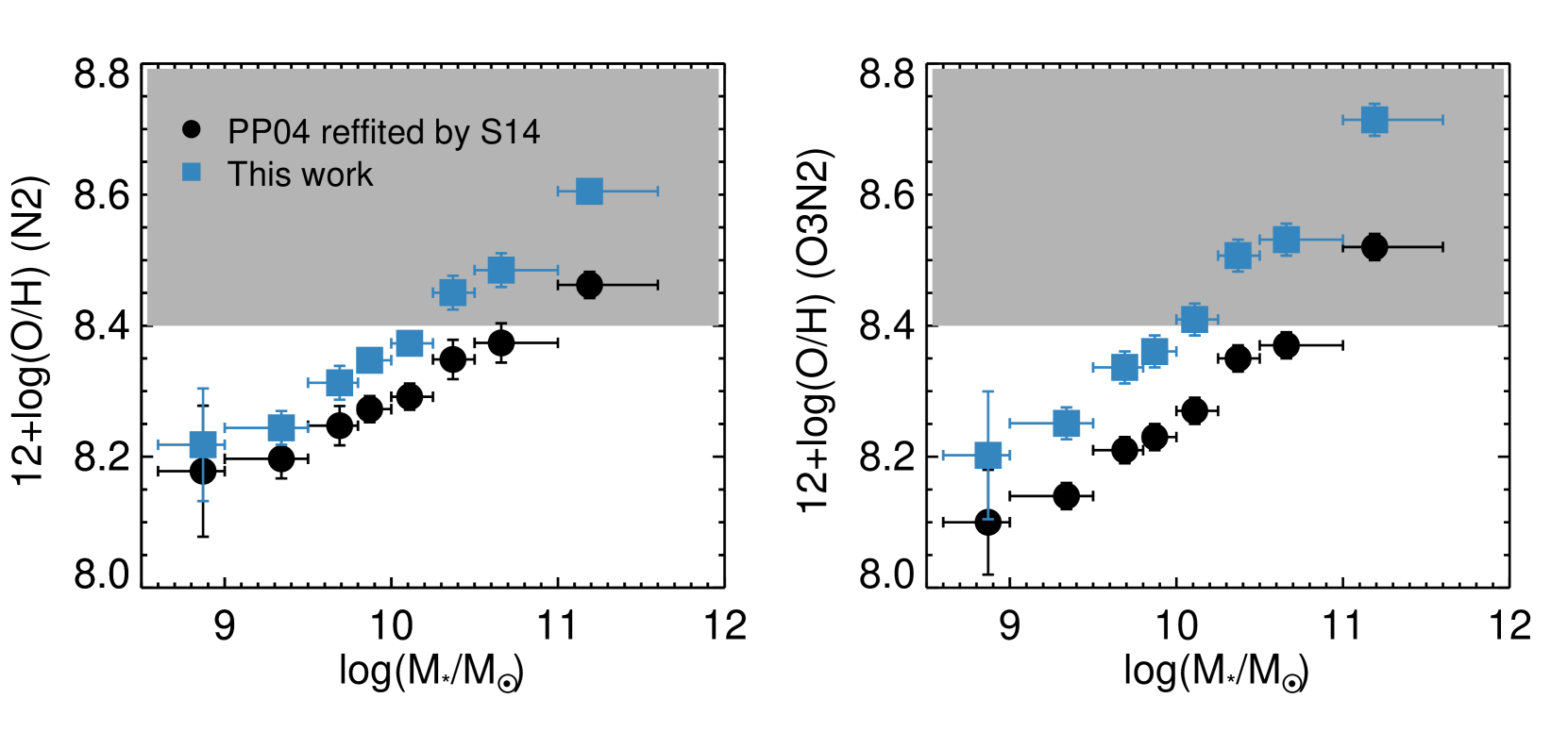
Figure 6: Mass-metallicity relation in $z\sim 2$ UV-selected star-forming galaxies (Steidel et al., 2016) based on the N2 (left) and O3N2 (right) diagnostics using the PP04 relation that was refitted by Steidel et al. (2014) (black data points) and the BKD18 (blue data points) calibrations. The shaded region represents the metallicity ranges that are out of the BKD18 calibration fitting range.

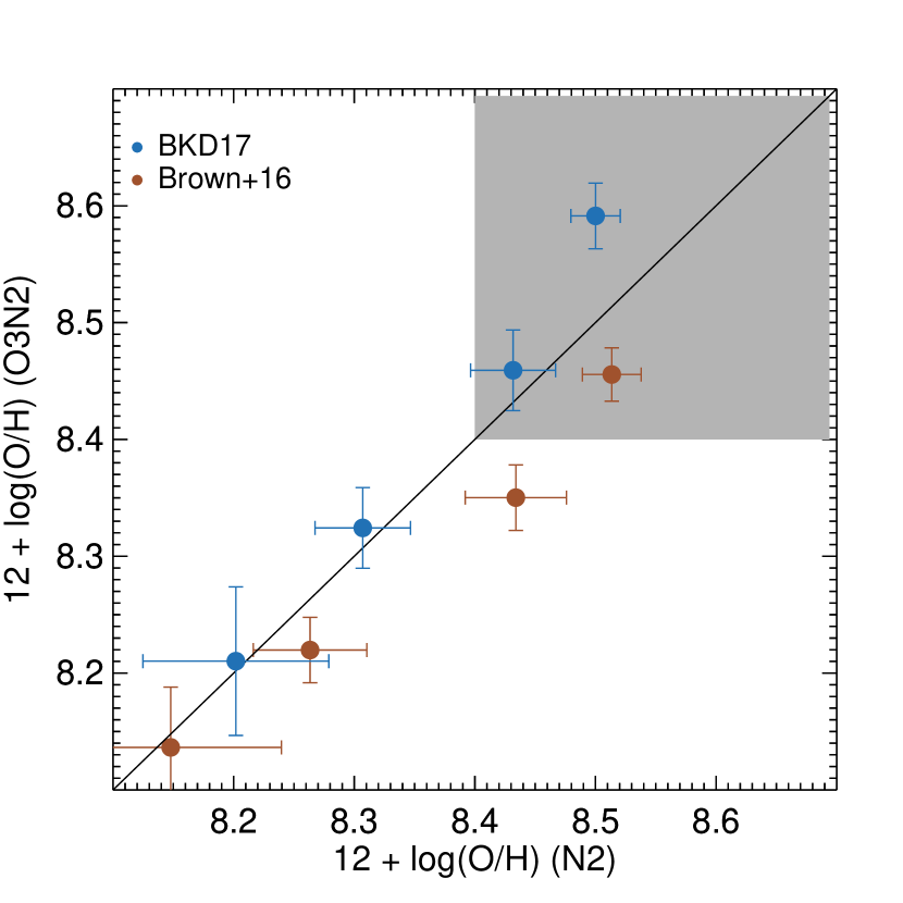
Figure 7: Comparison between the N2-based metallicity and O3N2-based metallicity in $z\sim 2$ star-forming galaxies using the BKD18 (blue data points) and Brown et al. (2016, brown data points) calibrations. The solid line represents the one-to-one relation between the N2 and O3N2 metallicity. The shaded region represents the metallicity range in which the BKD18 calibrations are not valid. The BKD18 calibrations are valid in the metallicity range $7.8<12+\log(\rm O/\rm H)<8.4$. In this metallicity range, the N2 and O3N2 metallicities in the BKD18 calibrations are more consistent with each other than the Brown et al. (2016) calibration.

5 Discussion

In this section, we refer to our new metallicity calibration based on the local analogs of high-redshift galaxies as the BKD18 calibration to simplify the expression.

5.1 Implications for High-redshift Galaxy Metallicity Measurements

The PP04 metallicity diagnostics cause a discrepancy between the N2 and O3N2 metallicities in $z\sim 2$ star-forming galaxies. The O3N2-based metallicity is systematically smaller than the N2-based metallicity by $0.10-0.15$ dex (e.g., Hainline et al., 2009; Bian et al., 2010; Newman et al., 2014; Steidel et al., 2014; Sanders et al., 2015). This discrepancy is primarily due to the offset between the local and $z\sim 2$ star-forming galaxies in the [O III]$\lambda$5007/H$\beta$ and [N II]$\lambda$6584/H$\alpha$ BPT diagram. Various physical mechanisms have been proposed to interpret this offset, including changes of ionization parameters, electron densities, radiation fields, and nitrogen-to-oxygen ratio over cosmic time. These proposed physical mechanisms are crucial input parameters for photoionization models and play an important role for the metallicity estimations. Our stacked spectra also shed light on what is the major physical mechanism(s) to drive the offset between high-redshift and low-redshift galaxies on the BPT diagram (F. Bian in preperation).

To test our new calibrations in high-redshift galaxies, we apply the BKD18 N2 and O3N2 empirical metallicity calibrations (equations 11 and 12) to two samples of $z\sim 2$ star-forming galaxies. One sample is selected based on their UV emission properties, UV-selected star-forming galaxies from Steidel et al. (2014), and the other is selected based on their stellar mass, mass-selected star-forming galaxies from Sanders et al. (2015). The local analog selection criteria in this work are based on the location of the UV-selected galaxies on the BPT diagram. Therefore, the ISM conditions in our local analogs are more representative to those in the UV-selected galaxies, and the BKD18 metallicity calibration is more suitable for this type of galaxy. Figure 5 shows the comparison between the N2- and O3N2-based metallicities in these UV-selected galaxies (blue filled circles) using our new metallicity calibrations. In the metallicity range of $8.1<\log(\rm{O/H})<8.4$ (shaded region in Figure 5), the mean difference between the BKD18 N2- and O3N2-metallicity is -0.03 dex. For a comparison, the mean difference between the PP04 N2- and O3N2-metallicity is 0.13 dex. The BKD18 calibrations successfully solve the discrepancy between N2- and O3N2-based metallicity when applying local PP04 calibrations to high-redshift galaxies (e.g., Steidel et al., 2014). The UV-selected star-forming galaxies may only represent $50\%-70\%$ of the whole population of high-redshift star-forming galaxies (Reddy et al., 2005). Therefore, we also apply our metallicity calibrations to a sample of mass-selected galaxies (Sanders et al., 2015), which is a more representative sample of $z\sim 2$ star-forming galaxies. Shapley et al. (2015) found that the [O III]/H$\beta$ ratio in mass-selected star-forming galaxies is not as high as UV-selected star-forming galaxies at $z\sim 2$, i.e., the BPT locus of mass-selected galaxies is lower than the BPT locus of UV-selected galaxies at $z\sim 2$. Our local analogs, therefore, may not fully resemble the ISM conditions of mass-selected galaxies, which could introduce systematical uncertainty when applying the new calibrations to mass-selected galaxies. In Figure 5, we plot the new N2- and O3N2-based metallicity based on the four stacked spectra of the mass-selected galaxies from Sanders et al. (2016b). In the metallicity range of $8.1<\log(\rm{O/H})<8.4$, the mean difference between the BKD18 N2- and O3N2-metallicity is -0.02 dex for mass-selected star-forming galaxies. For comparison, the mean difference between the PP04 N2- and O3N2-metallicity is 0.08 dex. Though the $z\sim 2$ mass-selected galaxies is slight offset from the $z\sim 2$ UV-selected galaxies on the BPT diagram (e.g., Figure 1(a) in Bian et al., 2017), the BKD18 calibrations are also suitable for $z\sim 2$ mass-selected galaxies.

It is worth noting that the N2 metallicity becomes systematically larger than the O3N2 metallicity in the BKD18 metallicity calibration, when $12+\log(\rm{O/H})>8.4$. The discrepancy increases when metallicity becomes larger. At $12+\log(\rm{O/H})=8.6$, the O3N2 metallicity is about 0.1 dex higher than N2 metallicity. This discrepancy suggests that the BKD18 calibration is not suitable for high-metallicity ($12+\log(\rm{O/H}>8.4$) cases. We do not recommend using the BKD18 calibration out of the metallicity range of $7.8<12+\log(\rm{O/H})<8.4$. It is difficult to use our local analogs to study the empirical calibration at $12+\log(\rm{O/H})>8.4$. The direct $T_{e}$ method becomes insensitive (or saturated) to the high-metallicity ($12+\log({\rm O/H})>8.5$) galaxies, because [O III]$\lambda$4363 is only emitted in the hottest nebulae, which biases toward the low-metallicity region. Therefore, the direct $T_{e}$ method underestimates the oxygen abundance in such galaxies.

The BKD18 metallicity calibrations provide a useful tool to study the mass-metallicity relation in high-redshift galaxies, particularly at the low-metallicity end. We measure metallicities in a sample of $z\sim 2$ star-forming galaxies from Steidel et al. (2014) using N2 and O3N2 indicators. Figure 6 shows the comparison between the mass-metallicity relation based on the BKD18 calibrations (blue squares) and that based on the PP04 calibrations (black circles). In the metallicity range of $8.0<Z<8.4$, we find that in both the N2 and O3N2 based- metallicities that the BKD18 calibrations are systematically higher than those based on the PP04 calibrations by 0.05 to 0.1 dex.

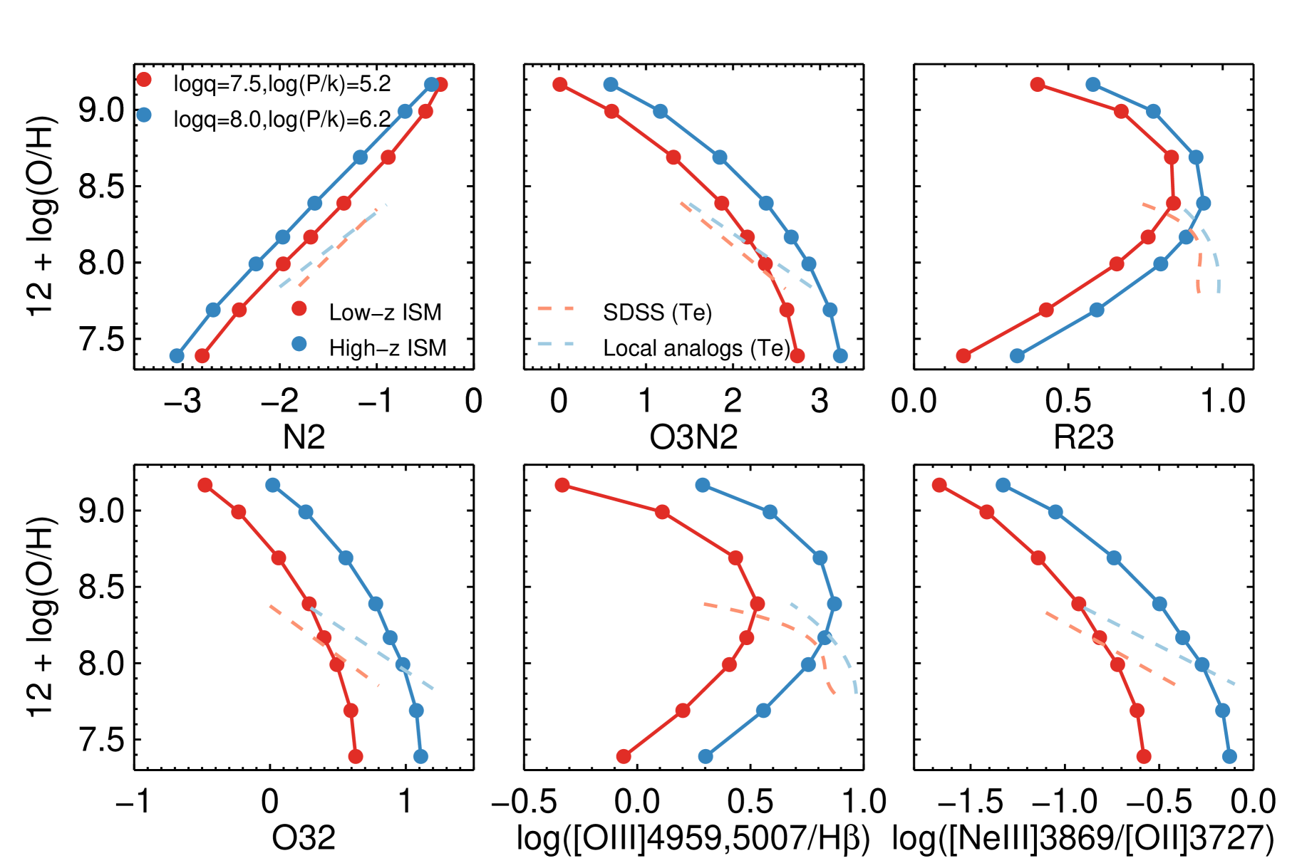
Figure 8: Relations between the strong emission-line ratios and oxygen abundance from MAPPINGs photoionization models. Two sets of model grids are displayed. The red filled circles denote the photoionization models with ISM pressure $\log(P/k)=5.2$ (electron density of $n_{e}\sim 10$) and photoionization parameter of $\log q=7.5$, which are representative values found in local star-forming galaxies. The blue filled circles denote the photoionization models with ISM pressure $\log(P/k)=6.2$ (electron density of $n_{e}\sim 100$) and photoionization parameter of $\log q=8.0$, which are comparable to those in $z\sim 2$ star-forming galaxies and our local analogs.The dashed lines represent the metallicity calibrations derived from the direct $T_{e}$ method in the SDSS reference galaxies (light red dashed line) and the local analogs of high-redshift galaxies (light blue dashed line).

5.2 Comparison with other high-redshift empirical metallicity calibrations

Recently, a few other studies have recalibrated the N2 and O3N2 metallicity for high-redshift galaxies (e.g., Brown et al., 2016; Cowie et al., 2016). Most of these studies used galaxies that are selected by matching their global properties to high-redshift galaxies, such as sSFRs (Brown et al., 2016) or H$\beta$ luminosities (Cowie et al., 2016). However, studies have shown that low-redshift galaxies selected by matching the global properties of high-redshift galaxies do not have the same ISM conditions as their high-redshift counterparts (e.g., Shirazi et al., 2014; Bian et al., 2016). Therefore, simply matching global properties may miss crucial information on the change of the ISM conditions, which play an important role in regulating the relation between metallicity and emission-line ratios. In Figure 7, we compare the N2- and O3N2-based metallicities in a sample of mass-selected star-forming galaxies at $z\sim 2$ from Sanders et al. (2015) using the BKD18 calibrations and the Brown et al. (2016) calibration. We adopt the measurements of the sSFR in the table 1 of Sanders et al. (2015). The mean difference between the Brown et al. (2016) calibration N2- and O3N2-metallicities is 0.05 dex. We find the BKD18 calibration results in the better consistency between the N2- and O3N2-metallicities compared with the Brown et al. (2016) calibration in the metallicity range of $8.1-8.4$.

5.3 Comparison with Photoionization Models

We study the evolution of the metallicity calibrations across the cosmic time by using the MAPPINGs photoionization models (Sutherland & Dopita, 1993; Dopita et al., 2013). We use the MAPPINGS IV code to generate the relation between the diagnostic line ratios and the oxygen abundance for two cases. In the first case, the input ionization parameter is $\log q=7.5$ and the ISM pressure is $\log(P/k)=5.2$, which corresponds to an electron density of $n_{e}\approx 10$ cm^-3. These parameters are comparable to those in the normal SDSS galaxies (e.g., Dopita et al., 2006; Nakajima & Ouchi, 2014; Bian et al., 2016). In the second case, the input ionization parameter is $\log q=8.0$ and the ISM pressure is $\log(P/k)=6.2$, which corresponds to an electron density of $n_{e}\approx 100$ cm^-3. These parameters are consistent with those in $z\sim 2$ galaxies and our local analogs (e.g., Nakajima & Ouchi, 2014; Bian et al., 2016; Kaasinen et al., 2017). Figure 8 shows the relations between the different diagnostic line ratios and the oxygen abundance derived from the photoionization models. The metallicity calibrations between the high-redshift and low-redshift conditions derived by the photoionization models (solid lines in Figure 8) follow the same trend as those between the local analogs and the SDSS reference galaxies (dashed lines in Figure 8). This suggests that the different metallicity calibration relations between the high- and low-redshift galaxies are due to the changes of the ISM conditions across cosmic time.

Although the $T_{e}$ metallicity and theoretical metallicity show the same relative trend for the dependence of ISM conditions for a given strong line ratio, the absolute metallicity derived from the direct $T_{e}$ method is significantly smaller than that from photoionization models by about 0.5 dex (see also Kewley & Ellison, 2008; Kewley, 2018). This discrepancy is mainly due to the (1) the Inhomogeneous temperature distribution in H II regions. The temperature fluctuation and/or gradients in H II regions bias the electron temperature measurements to the high temperature (low-metallicity) regions, thus the direct $T_{e}$ method underestimates the oxygen abundance. Futhuremore, (2) $\kappa$-distributions of electron energy in H II regions are also a factor. Nicholls et al. (2012) suggested that the electron energy in H II regions follows the $\kappa$-distributions rather than the Maxwell-Boltzmann distribution, and the electron temperatures derived based on the Maxwell-Boltzmann distribution are significantly higher than those from $\kappa$-distributions (Nicholls et al., 2013). Finally, (3) the relation between $t3$ (electron temperature in O⁺⁺ zone) and $t2$ (electron temperature in O⁺ zone) also plays a role. In this study, the $T_{e}$(O II)-$T_{e}$(O III) relation from Campbell et al. (1986) is adopted for a better comparison with previous studies. However, it is different from the $T_{e}$(O II)-$T_{e}$(O III) relation in the MAPPINGS photoionization models ($T_{e}$(O II)=0.685$T_{e}$(O III)+2100K Dopita et al., 2013)). The metallicities derived based on the $T_{e}$(O II)-$T_{e}$(O III) in the MAPPINGS photoionization models are 0.1-0.2 dex higher than the metallicities in this study. Meanwhile, the uncertainties of the input parameters in the photoionization models, particularly the shape of ionizing radiation field (e.g., Kewley et al., 2013a; Maier et al., 2014) and abundance scale (e.g., Steidel et al., 2014; Nicholls et al., 2017), can significantly affect the metallicity estimations. These parameters have not been well studied, particularly at high-redshift. Our local analogs of high-redshift galaxies providegreat opportunities to study what constrains these key input parameters in photoionization models (F. Bian et al. in preparation).

6 Conclusion

In this paper, we investigate the relations between the direct $T_{e}$-based metallicity and strong metallicity diagnostic line ratios in the stacked spectra of local analogs and normal SDSS galaxies. These analogs are selected to share the same location of $z\sim 2$ star-forming galaxies in the [O III]$\lambda$5007/H$\beta$ versus [N II]$\lambda$6584/H$\alpha$ BPT diagram. They closely resemble the interstellar medium properties, including high ionization parameters and electron densities, of $z\sim 2$ star-forming galaxies. These analogs provide a great opportunity to improve our understanding of the empirical metallicity calibrations in high-redshift galaxies. We summarize the main results of the paper as follows:

1. We select a sample of local analogs of high-redshift galaxies from the SDSS survey, which is located on the $z\sim 2.0$ star-formation sequence on the BPT diagram. The ionization parameters and electron densities in these analogs are comparable to those in $z\sim 2$ star-forming galaxies. Moreover, these galaxies show the exact the same behaviors relative to the local star-forming galaxies in different diagnostic diagrams. We also select a sample reference galaxies for a comparison.

2. We generate a series of stacked spectra for the sample of local analogs and SDSS reference galaxies in different $N2=\log$([N II]$\lambda$6584/H$\alpha$) bins. With the high S/N [O III]$\lambda$4363 detected in the stacked spectra, we measure the oxygen abundance based on the direct $T_{e}$ method.

3. We establish relations between the direct $T_{e}$ oxygen abundance and the N2 ($\log$([N II]$\lambda$6584/h$\alpha$)) and O3N2 ($\log$(([O III]$\lambda$5007/H$\beta$)/([N II]$\lambda$6584/H$\alpha$))) indicators for the local analogs and SDSS galaxies in the reference sample. The relations in the local analogs of high-redshifts do not follow those in the SDSS reference galaxies. This new empirical calibration is suitable to measure metallicity in high-redshift galaxies.

4. We build up the relation between the direct $T_{e}$ oxygen abundance and other metallicity indicators, including R23, O32, $\log($[O III]$\lambda\lambda$4959,5007/H$\beta$), and $\log$([Ne III]$\lambda$3869/[O II]$\lambda$3727) indices, in our local analogs, which can be used to measure metallicity in high-redshift galaxies.

5. We apply the new empirical calibrations based on our local analogs to a sample of star-forming galaxies at $z\sim 2$. Our new N2 and O3N2 empirical calibrations minimize the systematic discrepancy between the N2-based and O3N2-based metallicities in the star-forming galaxies at $z\sim 2$. The N2 and O3N2 metallicities will be underestimated by 0.05-0.1 dex, if one simply applies the local metallicity calibration to high-redshift galaxies.

6. By comparing our results with the MAPPINGS photoionization models, we find that the ISM conditions, including ionization parameter and electron density, play important roles in metallicity measurements.

References

- Abazajian et al. (2009) Abazajian, K. N., Adelman-McCarthy, J. K., Agüeros, M. A., et al. 2009, ApJS, 182, 543
- Andrews & Martini (2013) Andrews, B. H., & Martini, P. 2013, ApJ, 765, 140
- Baldwin et al. (1981) Baldwin, J. A., Phillips, M. M., & Terlevich, R. 1981, PASP, 93, 5
- Bian et al. (2017) Bian, F., Kewley, L. J., Dopita, M. A., & Blanc, G. A. 2017, ApJ, 834, 51
- Bian et al. (2016) Bian, F., Kewley, L. J., Dopita, M. A., & Juneau, S. 2016, ApJ, 822, 62
- Bian et al. (2010) Bian, F., Fan, X., Bechtold, J., et al. 2010, ApJ, 725, 1877
- Brinchmann et al. (2004) Brinchmann, J., Charlot, S., White, S. D. M., et al. 2004, MNRAS, 351, 1151
- Brinchmann et al. (2008) Brinchmann, J., Pettini, M., & Charlot, S. 2008, MNRAS, 385, 769
- Brown et al. (2016) Brown, J. S., Martini, P., & Andrews, B. H. 2016, MNRAS, 458, 1529
- Bruzual & Charlot (2003) Bruzual, G., & Charlot, S. 2003, MNRAS, 344, 1000
- Campbell et al. (1986) Campbell, A., Terlevich, R., & Melnick, J. 1986, MNRAS, 223, 811
- Cardelli et al. (1989) Cardelli, J. A., Clayton, G. C., & Mathis, J. S. 1989, ApJ, 345, 245
- Chabrier (2003) Chabrier, G. 2003, PASP, 115, 763
- Christensen et al. (2012) Christensen, L., Richard, J., Hjorth, J., et al. 2012, MNRAS, 427, 1953
- Cid Fernandes et al. (2005) Cid Fernandes, R., Mateus, A., Sodré, L., Stasińska, G., & Gomes, J. M. 2005, MNRAS, 358, 363
- Cowie et al. (2016) Cowie, L. L., Barger, A. J., & Songaila, A. 2016, ApJ, 817, 57
- Cullen et al. (2016) Cullen, F., Cirasuolo, M., Kewley, L. J., et al. 2016, MNRAS, 460, 3002
- Curti et al. (2017) Curti, M., Cresci, G., Mannucci, F., et al. 2017, MNRAS, 465, 1384
- Davé et al. (2012) Davé, R., Finlator, K., & Oppenheimer, B. D. 2012, MNRAS, 421, 98
- Dopita et al. (2016) Dopita, M. A., Kewley, L. J., Sutherland, R. S., & Nicholls, D. C. 2016, Ap&SS, 361, 61
- Dopita et al. (2013) Dopita, M. A., Sutherland, R. S., Nicholls, D. C., Kewley, L. J., & Vogt, F. P. A. 2013, ApJS, 208, 10
- Dopita et al. (2006) Dopita, M. A., Fischera, J., Sutherland, R. S., et al. 2006, ApJ, 647, 244
- Erb et al. (2006) Erb, D. K., Shapley, A. E., Pettini, M., et al. 2006, ApJ, 644, 813
- Ferland et al. (2013) Ferland, G. J., Porter, R. L., van Hoof, P. A. M., et al. 2013, RMxAA), 49, 137
- Finlator & Davé (2008) Finlator, K., & Davé, R. 2008, MNRAS, 385, 2181
- Garnett (1992) Garnett, D. R. 1992, AJ, 103, 1330
- Greene & Ho (2004) Greene, J. E., & Ho, L. C. 2004, ApJ, 610, 722
- Gunn et al. (2006) Gunn, J. E., Siegmund, W. A., Mannery, E. J., et al. 2006, AJ, 131, 2332
- Guo et al. (2016) Guo, Y., Koo, D. C., Lu, Y., et al. 2016, ApJ, 822, 103
- Hainline et al. (2009) Hainline, K. N., Shapley, A. E., Kornei, K. A., et al. 2009, ApJ, 701, 52
- Hirschmann et al. (2017) Hirschmann, M., Charlot, S., Feltre, A., et al. 2017, ArXiv e-prints, arXiv:1706.00010
- Izotov et al. (2006) Izotov, Y. I., Stasińska, G., Meynet, G., Guseva, N. G., & Thuan, T. X. 2006, A&A, 448, 955
- James et al. (2014) James, B. L., Pettini, M., Christensen, L., et al. 2014, MNRAS, 440, 1794
- Jones et al. (2015) Jones, T., Wang, X., Schmidt, K. B., et al. 2015, AJ, 149, 107
- Kaasinen et al. (2017) Kaasinen, M., Bian, F., Groves, B., Kewley, L. J., & Gupta, A. 2017, MNRAS, 465, 3220
- Kauffmann et al. (2003a) Kauffmann, G., Heckman, T. M., White, S. D. M., et al. 2003a, MNRAS, 341, 33
- Kauffmann et al. (2003b) Kauffmann, G., Heckman, T. M., Tremonti, C., et al. 2003b, MNRAS, 346, 1055
- Kewley (2018) Kewley, L. J. 2018, ARA&A, submitted
- Kewley & Dopita (2002) Kewley, L. J., & Dopita, M. A. 2002, ApJS, 142, 35
- Kewley et al. (2013a) Kewley, L. J., Dopita, M. A., Leitherer, C., et al. 2013a, ApJ, 774, 100
- Kewley et al. (2001) Kewley, L. J., Dopita, M. A., Sutherland, R. S., Heisler, C. A., & Trevena, J. 2001, ApJ, 556, 121
- Kewley & Ellison (2008) Kewley, L. J., & Ellison, S. L. 2008, ApJ, 681, 1183
- Kewley et al. (2006) Kewley, L. J., Groves, B., Kauffmann, G., & Heckman, T. 2006, MNRAS, 372, 961
- Kewley et al. (2013b) Kewley, L. J., Maier, C., Yabe, K., et al. 2013b, ApJ, 774, L10
- Kewley et al. (2016) Kewley, L. J., Yuan, T., Nanayakkara, T., et al. 2016, ApJ, 819, 100
- Kobulnicky & Kewley (2004) Kobulnicky, H. A., & Kewley, L. J. 2004, ApJ, 617, 240
- Kojima et al. (2016) Kojima, T., Ouchi, M., Nakajima, K., et al. 2016, ArXiv e-prints, arXiv:1605.03436
- Leitherer et al. (1999) Leitherer, C., Schaerer, D., Goldader, J. D., et al. 1999, ApJS, 123, 3
- Lilly et al. (2013) Lilly, S. J., Carollo, C. M., Pipino, A., Renzini, A., & Peng, Y. 2013, ApJ, 772, 119
- Liu et al. (2008) Liu, X., Shapley, A. E., Coil, A. L., Brinchmann, J., & Ma, C.-P. 2008, ApJ, 678, 758
- Lu et al. (2015) Lu, Y., Blanc, G. A., & Benson, A. 2015, ApJ, 808, 129
- Ly et al. (2016a) Ly, C., Malhotra, S., Malkan, M. A., et al. 2016a, ApJS, 226, 5
- Ly et al. (2014) Ly, C., Malkan, M. A., Nagao, T., et al. 2014, ApJ, 780, 122
- Ly et al. (2016b) Ly, C., Malkan, M. A., Rigby, J. R., & Nagao, T. 2016b, ApJ, 828, 67
- Ly et al. (2015) Ly, C., Rigby, J. R., Cooper, M., & Yan, R. 2015, ApJ, 805, 45
- Ma et al. (2016) Ma, X., Hopkins, P. F., Faucher-Giguère, C.-A., et al. 2016, MNRAS, 456, 2140
- Maier et al. (2014) Maier, C., Lilly, S. J., Ziegler, B. L., et al. 2014, ApJ, 792, 3
- Maiolino et al. (2008) Maiolino, R., Nagao, T., Grazian, A., et al. 2008, A&A, 488, 463
- Marino et al. (2013) Marino, R. A., Rosales-Ortega, F. F., Sánchez, S. F., et al. 2013, A&A, 559, A114
- Masters et al. (2014) Masters, D., McCarthy, P., Siana, B., et al. 2014, ApJ, 785, 153
- McGaugh (1991) McGaugh, S. S. 1991, ApJ, 380, 140
- Nagao et al. (2006) Nagao, T., Maiolino, R., & Marconi, A. 2006, A&A, 459, 85
- Nakajima & Ouchi (2014) Nakajima, K., & Ouchi, M. 2014, MNRAS, 442, 900
- Newman et al. (2014) Newman, S. F., Buschkamp, P., Genzel, R., et al. 2014, ApJ, 781, 21
- Nicholls et al. (2012) Nicholls, D. C., Dopita, M. A., & Sutherland, R. S. 2012, ApJ, 752, 148
- Nicholls et al. (2013) Nicholls, D. C., Dopita, M. A., Sutherland, R. S., Kewley, L. J., & Palay, E. 2013, ApJS, 207, 21
- Nicholls et al. (2017) Nicholls, D. C., Sutherland, R. S., Dopita, M. A., Kewley, L. J., & Groves, B. A. 2017, MNRAS, 466, 4403
- Onodera et al. (2016) Onodera, M., Carollo, C. M., Lilly, S., et al. 2016, ApJ, 822, 42
- Pagel et al. (1992) Pagel, B. E. J., Simonson, E. A., Terlevich, R. J., & Edmunds, M. G. 1992, MNRAS, 255, 325
- Pérez-Montero & Contini (2009) Pérez-Montero, E., & Contini, T. 2009, MNRAS, 398, 949
- Pettini & Pagel (2004) Pettini, M., & Pagel, B. E. J. 2004, MNRAS, 348, L59
- Pilyugin et al. (2012) Pilyugin, L. S., Grebel, E. K., & Mattsson, L. 2012, MNRAS, 424, 2316
- Pilyugin & Thuan (2005) Pilyugin, L. S., & Thuan, T. X. 2005, ApJ, 631, 231
- Pilyugin et al. (2010) Pilyugin, L. S., Vílchez, J. M., & Thuan, T. X. 2010, ApJ, 720, 1738
- Reddy et al. (2005) Reddy, N. A., Erb, D. K., Steidel, C. C., et al. 2005, ApJ, 633, 748
- Rigby et al. (2011) Rigby, J. R., Wuyts, E., Gladders, M. D., Sharon, K., & Becker, G. D. 2011, ApJ, 732, 59
- Rodighiero et al. (2011) Rodighiero, G., Daddi, E., Baronchelli, I., et al. 2011, ApJ, 739, L40
- Sanders et al. (2017) Sanders, R. L., Shapley, A. E., Zhang, K., & Yan, R. 2017, ArXiv e-prints, arXiv:1708.04625
- Sanders et al. (2015) Sanders, R. L., Shapley, A. E., Kriek, M., et al. 2015, ApJ, 799, 138
- Sanders et al. (2016a) —. 2016a, ApJ, 825, L23
- Sanders et al. (2016b) —. 2016b, ApJ, 816, 23
- Savaglio et al. (2005) Savaglio, S., Glazebrook, K., Le Borgne, D., et al. 2005, ApJ, 635, 260
- Shapley et al. (2015) Shapley, A. E., Reddy, N. A., Kriek, M., et al. 2015, ApJ, 801, 88
- Shaw & Dufour (1995) Shaw, R. A., & Dufour, R. J. 1995, PASP, 107, 896
- Shirazi et al. (2014) Shirazi, M., Brinchmann, J., & Rahmati, A. 2014, ApJ, 787, 120
- Smee et al. (2013) Smee, S. A., Gunn, J. E., Uomoto, A., et al. 2013, AJ, 146, 32
- Stark et al. (2013) Stark, D. P., Schenker, M. A., Ellis, R., et al. 2013, ApJ, 763, 129
- Steidel et al. (2016) Steidel, C. C., Strom, A. L., Pettini, M., et al. 2016, ApJ, 826, 159
- Steidel et al. (2014) Steidel, C. C., Rudie, G. C., Strom, A. L., et al. 2014, ApJ, 795, 165
- Stoughton et al. (2002) Stoughton, C., Lupton, R. H., Bernardi, M., et al. 2002, AJ, 123, 485
- Strauss et al. (2002) Strauss, M. A., Weinberg, D. H., Lupton, R. H., et al. 2002, AJ, 124, 1810
- Strom et al. (2017a) Strom, A. L., Steidel, C. C., Rudie, G. C., Trainor, R. F., & Pettini, M. 2017a, ArXiv e-prints, arXiv:1711.08820
- Strom et al. (2017b) Strom, A. L., Steidel, C. C., Rudie, G. C., et al. 2017b, ApJ, 836, 164
- Sutherland & Dopita (1993) Sutherland, R. S., & Dopita, M. A. 1993, ApJS, 88, 253
- Tremonti et al. (2004) Tremonti, C. A., Heckman, T. M., Kauffmann, G., et al. 2004, ApJ, 613, 898
- Vanzella et al. (2016) Vanzella, E., De Barros, S., Cupani, G., et al. 2016, ApJ, 821, L27
- Veilleux & Osterbrock (1987) Veilleux, S., & Osterbrock, D. E. 1987, ApJS, 63, 295
- Voges et al. (2000) Voges, W., Aschenbach, B., Boller, T., et al. 2000, VizieR Online Data Catalog, 9029, 0
- York et al. (2000) York, D. G., Adelman, J., Anderson, Jr., J. E., et al. 2000, AJ, 120, 1579
- Yuan & Kewley (2009) Yuan, T.-T., & Kewley, L. J. 2009, ApJ, 699, L161
- Zahid et al. (2014) Zahid, H. J., Dima, G. I., Kudritzki, R.-P., et al. 2014, ApJ, 791, 130
- Zahid et al. (2013) Zahid, H. J., Geller, M. J., Kewley, L. J., et al. 2013, ApJ, 771, L19
- Zhang et al. (2017) Zhang, K., Yan, R., Bundy, K., et al. 2017, MNRAS, 466, 3217