Cosmological constraints with self-interacting sterile neutrinos

Abstract

In this work we revisit the question of whether Cosmology can be made compatible with scenarios with light sterile neutrinos, as invoked to explain the SBL anomalies, in the presence of self-interaction among sterile neutrinos mediated by massive gauge bosons. We examine this proposal by deriving the cosmological predictions of the model in a wide range of the model parameters including the effective interaction strength $G_{X}$, sterile neutrino mass ${m_{\rm st}}$ and active-sterile mixings. With those we perform a statistical analysis of the cosmological data from BBN, CMB, and BAO data to infer the posterior probabilities of the sterile self-interaction model parameters. BBN mostly provides information about the effective interaction strength and we find that $\log_{10}(G_{X}/G_{F})\geq{4.0}$ can describe the primordial abundances at 95% CL. Our analysis of CMB and BAO data show that when allowing a wide prior for the sterile neutrino mass its posterior is bounded to ${m_{\rm st}}\leq{0.95}~{}{\rm eV}$ (95% CL) considering CMB data only and ${m_{\rm st}}\leq 0.37~{}{\rm eV}$ (95% CL) when adding the BAO information. So the mass bounds are slighly relaxed compared with that of a non-interacting sterile neutrino model but a sterile neutrino mass of 1 eV is still excluded at more than $2\sigma$ CL. Conversely if fixing the sterile neutrino mass and mixing to the values prefered by short baseline data we find that while that CMB data alone favors the self-interacting scenario, including the BAO information severly degrades the agreement with the model. Altogether we conclude then that adding the self-interaction can alleviate the tension between eV sterile neutrinos and CMB data, but when including also the BAO results the self-interacting sterile neutrino model cannot lead to a satisfactory description of the data.

1 Introduction

Over the last two decades it has been solidly established the need to extend the leptonic sector of the Standard Model with the addition of mass terms for at least two of its three neutrino states, as required to describe the results of solar, atmospheric, reactor and long baseline neutrino experiments (for a review see  [1]). In this extension, lepton flavors are not symmetries of Nature  [2, 3] and the minimum joint description of all these data requires mixing among all the three known neutrinos ($\nu_{e}$, $\nu_{\mu}$, $\nu_{\tau}$), which can be expressed as quantum superposition of three massive states $\nu_{i}$ ($i=1,2,3$) with masses $m_{i}$ leading to the observed oscillation signals with $\Delta m^{2}_{21}=(7.40\pm 0.21)10^{-4}$ eV² and $|\Delta m^{2}_{3\ell}|=(2.5\pm 0.03)\times 10^{-3}$ eV² and non-zero values of the three mixing angles [4, 5].

In addition to these well-established results, there remains a set of anomalies in neutrino data at relatively short-baselines (SBL). The first one came from the LSND experiment [6] which observed excess events of $\bar{\nu}_{\mu}\rightarrow\bar{\nu}_{e}$ oscillations. An excess was also observed in the antineutrino mode of MiniBooNE [7] which was consistent with the results of LSND, while the search for $\nu_{\mu}\rightarrow\nu_{e}$ oscillations reported excess only in the low energy range [8]. GALLEX [9, 10, 11] and SAGE [12] detected electron neutrinos produced by radioactive sources and observed deficit in the $\nu_{e}$ capture rates. The deficit is known as Gallium anomaly. Furthermore, some reactor antineutrino measurements also reported deficit in the $\bar{\nu}_{e}$ flux [13] in the near detectors. When interpreted in terms of oscillations, each of these anomalies pointed out towards a $\Delta m^{2}\sim{\cal O}({\rm eV}^{2})$ and mixing angle $\theta\sim 0.1$  [14, 15, 16, 17, 18, 19, 20, 21, 22, 23, 24] and consequently could not be explained within the context of the 3$\nu$ mixing described above. They required instead the addition of one or more neutrino states (what is usually referred to as $3+1$ or $3+N_{s}$ models) which must be sterile, i.e. elusive to Standard Model interactions, to account for the constraint of the invisible $Z$ width which limits the number of light weak-interacting neutrinos to be $2.984\pm 0.008$ [25].

Recently, some of these anomalies have been questioned, in particular with the results of new reactor neutrino experiments from Daya Bay [26], NEOS [27], and DANSS [28, 29, 30], together with theoretical developments in the calculation of reactor neutrino fluxes [31, 32]. But a combined analysis of Daya Bay data with NEOS and DANSS experiments still allows for eV sterile neutrinos [33, 34] to explain for disappearance of $\bar{\nu}_{e}$. Mounting tensions arise, however, to find a consistent description incorporating also the appearance results from LSND and MiniBoone [35].

Besides the debate on the status of these hints towards light sterile neutrinos in oscillation experiments, massive sterile neutrino itself have interesting consequences in Cosmology. If they have a non-negligible mixing with active neutrinos, light sterile neutrinos were in thermal equilibrium with the active neutrinos in the early universe which results in the effective number of neutrino species $N_{\mathrm{eff}}\simeq 4$ in the 3+1 models. This is in tension with the precise measurement of primordial abundances produced in Big Bang Nucleosynthesis (BBN) [36] and with Cosmic Microwave Background (CMB) data which generically constraints $N_{\mathrm{eff}}$ to be close to three, and the total mass of the neutrinos to be well below eV  [37].

The generic conclusion is that, in order to accommodate the cosmological observations within the $3+N_{s}$ scenarios motivated by SBL results, some new form of physics is required to suppress the contribution of the sterile neutrinos to $N_{\mathrm{eff}}$ (see for example [38]). Among others extended scenarios with a time varying dark energy component [39], entropy production after neutrino decoupling [40], very low reheating temperature [41], large lepton asymmetry [42, 43, 44], and non-standard neutrino interactions  [45, 46, 47], have been considered. All these mechanisms have the effect of diluting the sterile neutrino abundance or suppressing its production in the early universe. In particular the presence of new interactions in the sterile sector have been proposed to achieve this goal. The interactions via a light pseudoscalar for the 4th mass state has been studied by Archidiacono et al [48, 49] which lead to a consistent description of cosmological observations including an upward revision of Hubble constant $H_{0}$. However, in their work the interaction strength was not mapped into $N_{\mathrm{eff}}$ directly due to the complexity of the quantum kinetic equations (QKEs). Alternatively in Refs. [46, 50] it was proposed that new interaction between sterile neutrinos mediated by a new massive gauge boson $X$ described by a Lagrangian

$$\mathcal{L}_{\rm int}=g_{X}\bar{\nu}_{s}\gamma_{\mu}\dfrac{1}{2}(1-\gamma_{5})\nu_{s}X^{\mu}\,,$$ (1.1)

where $g_{X}$ is the gauge coupling. When the energy scale is smaller than the gauge boson mass $M_{X}$, we can integrate $X$ out to obtain an effective four sterile neutrino interaction Lagrangian with the effective coupling $\frac{G_{X}}{\sqrt{2}}=\frac{g_{X}^{2}}{8M_{X}^{2}}$. This new interaction has been studied by Saviano et al to obtain the bounds from BBN [51] as well as CMB and baryon acoustic oscillation (BAO) data [52], and most recently in Ref. [53] from future measurements of the diffuse supernova background. In particular in Refs. [51, 52] it is argued that this new interaction can reduce $N_{\mathrm{eff}}$ to 2.7 via a late production of sterile neutrinos. And with a large coupling it can reduce the free-steaming of neutrinos, which can induce changes in the amplitude and phase of the acoustic peaks in the CMB spectrum [54], and avoid the constraint on $\Sigma m_{\nu}$ from the measurement of large scale structure. Still, the study in Ref. [52] showed that the strong self-interacting scenario described in Ref. [50] is excluded by more than 3$\sigma$ (see also Ref. [55] for a recent discussion).

In this work, we have a critical look at the proposal of such vector-like sterile neutrino self-interactions without focusing on the representative strong-interacting scenario but rather exploring a large range of effective couplings from weak to strong. Our aim is to show to what extent this new interaction can or cannot alleviate the tension between light sterile neutrinos and Cosmology. Technically our work relies on the formalism developed in Refs. [56, 52] to account for the new sterile neutrino self-interactions in the QKE for the density of the neutrino ensemble, and in the Boltzmann equations for its perturbations (to which we introduce some minor improvements) but we differ from Refs. [56, 52] in the assumptions used when obtaining the energy and phase space distributions of the neutrino ensemble after decoupling (the corresponding value of $N_{\mathrm{eff}}$) as discussed in Sec. 2. Furtherore, we extend the study by consistently exploring the solutions obtained as a function of the parameters of the sterile neutrino self-interacting model. With those at hand we perform a Bayesian analysis of the cosmological data from BBN, CMB, and BAO data to infer the posterior of the sterile self-interaction model parameters in Sec. 3. We summarize our conclusions in Sec. 4. We include an appendix with two short sections describing the possible dependence of the results on the priors implied for $N_{\mathrm{eff}}$ and on the range of validity of the study.

2 Framework

Our starting point is a $\Lambda$CDM cosmology extended with one additional sterile neutrino with mass ${m_{\rm st}}$ with non-zero projections over two of the massive neutrino states (as parametrized by two mixing angles $\theta_{14}$ and $\theta_{24}$) with self-interactions as in Eq. (1.1) with coupling constant $g_{X}$ mediated by a massive boson of mass $M_{X}$ (or equivalently with an effective self-coupling $G_{X}$). For each point in the model parameter space ${m_{\rm st}}$, $\theta_{14}$, $\theta_{24}$, $g_{X}$, and $G_{X}$ we first obtain the effective number of neutrino species at the time of BBN $N_{\mathrm{eff}}(T_{\rm BBN})$ by solving the QKEs quantifying the neutrino flavour evolution as described in Secs. 2.1 and 2.2. Subsequently we consistently introduce both the results of the QKE’s relevant for the neutrino background evolution and the direct effect of the sterile neutrino self-interactions in the Boltzmann equations for the neutrino perturbations as described in Sec. 2.3 and obtain the modified predictions for CMB and BAO observables.

2.1 Sterile neutrino production and neutrino flavor evolution

In the early universe the self-interactions in Eq. (1.1) induce inelastic collisions among the sterile states with rate

$$\Gamma_{X}=n_{\nu_{s}}\langle\sigma v\rangle\simeq G_{X}^{2}T_{\nu_{s}}^{5}\;,$$ (2.1)

where $n_{\nu_{s}}$ and $T_{\nu_{s}}$ are the number density and temperature of the sterile neutrinos. Because of the mixing between sterile neutrinos and active neutrinos these collisions can bring the sterile neutrinos into thermal equilibrium with the active ones.

However the self-interactions also induce elastic forward scattering among the sterile neutrinos which can be parametrized in terms of an MSW-like [57] effective potential which takes the form  [58]

$$V_{\rm eff}=-\dfrac{8\sqrt{2}G_{X}\,p\,\varepsilon_{s}}{3M_{X}^{2}}\,,$$ (2.2)

where $p$ is the momentum of the sterile neutrino and $\varepsilon_{s}$ is its energy density. As discussed in Refs. [46, 50] by introducing this effective potential the in-medium mixing angle between active and sterile neutrinos deviates from its vacuum value by

$$\sin^{2}2\theta_{m}\,=\,\dfrac{\sin^{2}2\theta_{0}}{\left(\cos 2\theta_{0}\,+\,2E/{m_{\rm st}}^{2}\,{V_{\rm eff}}\right)^{2}\,+\,\sin^{2}2\theta_{0}}\,,$$ (2.3)

So if ${V_{\rm eff}}\gg f_{\rm osc}={m_{\rm st}}^{2}/(2E)$ before neutrinos decoupling from the primordial plasma, the in-medium mixing angle is highly suppressed and sterile neutrino production is deferred until after decoupling. By comparing the interaction rate with the expansion rate, and the self-interaction potential with the oscillation frequency, one finds that this mechanism can work for strong enough interactions.

However it was argued in Ref. [59] that entropy should be conserved after decouling so the entropy possessed by the three active neutrino species had to be shared with the sterile neutrinos. This assumption leads to a reduction in the total neutrino energy density which implies that $N_{\mathrm{eff}}$ could be as low as 2.7 instead of 4. A value which would be too low when confronted with data  [52] unless some additional mechanism besides mixing was invoked to produce the sterile neutrinos [50]. As we discuss below we depart from the entropy conservation assumption employed in Ref. [59] when evaluating $N_{\mathrm{eff}}$ which may affect the conclusions about this scenario in the strong coupling regime as we describe next.

The quantitative determination of $N_{\mathrm{eff}}$ in scenarios with light sterile neutrinos which are brought in to equilibrium by their mixing with the standard three active neutrinos requires to evaluate the time evolution of their energy density. To do so we can use the quantum kinetic equations (QKEs) of the 3+1 neutrino ensemble described in Ref. [56]. For sake of completeness we briefly summarize them here with the inclusion of two minor improvements: considering a separate treatment of neutrino and photon temperature, and an improved determination of the electron energy density.

The flavour evolution of the 3+1 neutrino ensemble is described in terms of a 4x4 density matrix $\varrho(p,t)$ whose evolution is governed by the QKEs

$${\rm i}\,\frac{d\varrho}{dt}=[\Omega,\varrho]+C[\varrho]\,,$$ (2.4)

where $C[\varrho]$ represents the collision terms while the oscillation and in-medium potential terms corresponding to charged current ($CC$) interactions with the background electrons and the neutral current ($NC$) interactions with the background neutrinos are

$$\Omega=\dfrac{1}{2p}U^{\dagger}M^{2}U+\sqrt{2}G_{F}\left[-\dfrac{8p}{3}\left(\dfrac{{\cal E}_{l}}{M_{W}^{2}}+\dfrac{{\cal E}_{\nu}}{M_{Z}^{2}}\right)\right]+\sqrt{2}G_{X}\left[-\dfrac{8p}{3}\dfrac{{\cal E}_{s}}{M_{X}^{2}}\right]\,.$$ (2.5)

$M^{2}=\mathrm{diag}(0,\Delta m_{21}^{2},\Delta m_{31}^{2},m_{\rm st}^{2})$ (we assume the sterile neutrino mass is much larger than the active ones), and $M_{W}$ and $M_{Z}$ are the masses of $W$ and $Z$ bosons respectively. $U=R_{34}R_{24}R_{23}R_{14}R_{13}R_{12}$ ($R_{ij}$ representing a rotation of angle $\theta_{ij}$ in the ${ij}$ plane) is the neutrino mixing matrix.

In what follows we fix the oscillation parameters for the three active neutrinos $\Delta m^{2}_{21}$, $\Delta m^{2}_{31}$, $\theta_{12}$ , $\theta_{13}$, and $\theta_{23}$ to the best fit for normal ordering from the global oscillation analysis in NuFIT 3.0  [4, 5]. In Eq. (2.5) ${\cal E}_{l}=\mathrm{diag}(\varepsilon_{e},0,0,0)$, ${\cal E}_{\nu}$, and ${\cal E}_{s}=\mathrm{diag}(0,0,0,\varepsilon_{s})$ are $4\times 4$ matrices containing the energy density of the electrons, active neutrinos (which is in general non-diagonal with non-zero entries in the upper $3\times 3$ sector), and sterile neutrinos respectively.

Equation  (2.4), though well-defined, is extremely computationally demanding due to the momentum dependence of the density matrix, especially in the case of three active plus one sterile neutrino species. To retain the main features of the flavor evolution within a reasonable amount of computing time, we still resort to the average momentum approximation as described in [56]. In this approximation, ones remove the momentum dependence in the equations by assuming

$$\varrho(x,y)\longrightarrow f_{\rm FD}(y)\rho(x)\;,$$ (2.6)

where $f_{\rm FD}$ Fermi-Dirac distribution function for the neutrinos and for convenience we have introduced the dimensionless variables

$$x\equiv ma,\quad y\equiv pa,\quad z_{\gamma}\equiv T_{\gamma}a,\quad z_{\nu}\equiv T_{\nu}a,$$ (2.7)

where we take the arbitrary mass scale $m$ to be 1 MeV. This assumes neutrinos are featured by grey body Fermi-Dirac distributions. We shall use Eq. (2.6) later to restore the momentum dependent phase space distribution of neutrinos. We stress that we have added $z_{\nu}$ to trace the difference between neutrino and photon temperatures at or after the time of $e^{+}e^{-}$ annihilation. Since we are solving the equations below $\mu^{+}\mu^{-}$ annihilation, always $T_{\nu}\propto 1/a$ so $z_{\nu}$ is a constant (hence the $f_{\rm FD}$ in Eq. (2.6) is only a function of $y$). In what follows we normalize the scale factor to $a(t)=1/T_{\nu}$ so that $z_{\nu}(x)$ is always 1. However $z_{\gamma}$ will evolve. Indeed we can solve for $z_{\gamma}(x)$ from the conservation of stress-energy tensor (see Eq. (15) in [60] for a detailed treatment). The solution does not depend on the details of the neutrino flavor evolution, so this $z_{\gamma}(x)$ is precomputed as a known function before solving the QKEs.

Altogether one finds

$$i\dfrac{d\rho}{dx}= + \dfrac{x^{2}}{2m^{2}\widetilde{H}}\langle\dfrac{1}{y}\rangle\left[U^{\dagger}M^{2}U,\rho\right]+\dfrac{\sqrt{2}G_{F}m^{2}}{x^{2}\widetilde{H}}\left[\left(-\dfrac{8\langle y\rangle m^{2}}{3x^{2}M_{W}^{2}}\widetilde{\cal E}_{l}-\dfrac{8\langle y\rangle m^{2}}{3x^{2}M_{Z}^{2}}\widetilde{\cal E}_{\nu}\right),\rho\right]$$ (2.8)

$$+ \dfrac{\sqrt{2}G_{X}m^{2}}{x^{2}\widetilde{H}}\left[-\dfrac{8\langle y\rangle m^{2}}{3x^{2}M_{X}^{2}}\widetilde{\cal E}_{s},\rho\right]+\dfrac{x\langle C[\rho]\rangle}{m\widetilde{H}}\,,$$

where in the potentials

$$\widetilde{\cal E}_{l} = \mathrm{diag}(\tilde{\varepsilon}_{e},0,0,0)\,,$$ (2.9)

$$\widetilde{\cal E}_{\nu} = \dfrac{2}{2\pi^{2}}\int_{0}^{\infty}dyy^{3}G_{s}\varrho(x,y)G_{s}=\dfrac{7}{8}\dfrac{\pi^{2}}{15}G_{s}\rho(x)G_{s}\,,$$ (2.10)

$$\widetilde{\cal E}_{s} = \dfrac{2}{2\pi^{2}}\int_{0}^{\infty}dyy^{3}G_{sX}\varrho(x,y)G_{sX}=\dfrac{7}{8}\dfrac{\pi^{2}}{15}G_{sX}\rho(x)G_{sX}\,.$$ (2.11)

In the above equations $G_{s}=\mathrm{diag}(1,1,1,0)$ and $G_{sX}=\mathrm{diag}(0,0,0,1)$ contain the dimensionless coupling constants for active and sterile neutrinos, respectively. We have introduced the normalized Hubble parameter as

$$\widetilde{H}\equiv\dfrac{x^{2}}{m}H=\dfrac{m}{M_{\rm Pl}}\sqrt{\dfrac{8\pi\tilde{\varepsilon}(x,z_{\gamma}(x),z_{\nu}(x))}{3}}\,,$$ (2.12)

where $M_{\rm Pl}$ is the Planck mass and the comoving total energy density is defined as $\tilde{\varepsilon}\equiv\varepsilon(x/m)^{4}$ with $\varepsilon=\tilde{\varepsilon}_{e}+{\rm Tr}(\widetilde{\cal E}_{\nu}+\widetilde{\cal E}_{s})$ is the total energy density. If we define the “reference” cosmological model as the $\Lambda{\rm CDM}$ model plus three active neutrinos, in this model neutrinos keep in thermal equilibrium with the plasma until decoupling. After $e^{+}e^{-}$ annihilation, $T_{\nu}=(4/11)^{1/3}T_{\gamma}$. The number density of a neutrino species in the reference model is denoted by $n_{\nu}^{*}$. In terms of the average momentum approximation, the diagonal entries in the density matrix denote the number density of active or sterile neutrinos normalized to $n_{\nu}^{*}$.

Also when computing $\tilde{\varepsilon}_{e}$ we use

$$\tilde{\varepsilon}_{e}=\dfrac{2}{\pi^{2}}\int_{0}^{\infty}dyy^{3}{f_{\rm FD}}_{e}(y,z_{\gamma}(x)),$$ (2.13)

with ${f_{\rm FD}}_{e}=g_{e}/\exp(\sqrt{y^{2}+x^{2}m_{e}^{2}/m^{2}}/z_{\gamma}+1)$ which is slightly different from from Eq. (18) in Ref. [56] in that we keep the electron mass so the energy density of electrons quickly approaches 0 during annihilation.

In Eq. (2.8), $\langle C[\varrho]\rangle$ is the momentum average of active and sterile collision terms expressed as [43, 56]

$$\langle C_{\nu}[\varrho]\rangle = -\dfrac{i}{2}G_{F}^{2}\dfrac{m^{5}}{x^{5}}(\{S^{2},\rho-I\}-2S(\rho-I)S+\{A^{2},\rho-I\}+2A(\rho-I)A\,,$$

$$\langle C_{s}[\varrho]\rangle = -\dfrac{i}{2}G_{X}^{2}\dfrac{m^{5}}{x^{5}}(\{S_{X}^{2},\rho-I\}-2S_{X}(\rho-I)S_{X})\,,$$ (2.14)

where the active neutrino scattering and annihilation matrix $S=\mathrm{diag}(g_{s}^{e},g_{s}^{\mu},g_{s}^{\tau},0)$ and $A=\mathrm{diag}(g_{a}^{e},g_{a}^{\mu},g_{a}^{\tau},0)$ with $(g_{s}^{e})^{2}=3.06$, $(g_{a}^{e})^{2}=0.50$, $(g_{s}^{\mu,\tau})^{2}=2.22$, and $(g_{a}^{\mu,\tau})^{2}=0.28$  [43] while for sterile neutrinos $S_{X}=\mathrm{diag}(0,0,0,1)$. We always work in the approximation $T_{\nu}<M_{X}$ so annihilation terms are neglected we lose the details of the phase-space distribution, so we always assume all neutrino species share the same temperature when solving the QKEs. This assumption is robust since even if there are small differences between the temperature of the different neutrino species, the in-medium potentials are only corrected by factors of ${\cal O}(1)$ and the solution of the QKEs would be barely changed.

We solve these equations for an array of values of the model parameters ${m_{\rm st}}$, $\theta_{14}$, and $\theta_{24}$ (for simplicity we neglect mixing $\theta_{34}$), $g_{X}$ and $G_{X}$ (or equivalently $M_{X}$) and obtain as a solution $\rho(T_{\nu})$. As illustration of the output of the QKEs we show in Fig. 1 an example of the neutrino flavor evolution with parameters such that the new interaction is much stronger than electroweak interactions. As one would expect, sterile neutrinos are produced only when the temperature is well below 1 MeV and all four neutrino species get to similar number densities after thermalization. For comparison we show in the right panel the neutrino flavor evolution in the absence of new interactions. In this case sterile neutrinos get immediately thermalized with the active neutrinos. It clearly shows that the self-interaction among sterile neutrinos, when strong enough, is capable of postponing their production until after active neutrino decoupling.

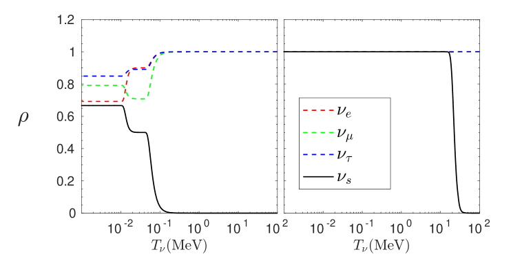
Figure 1: The number density $\rho_{\alpha\alpha}$ of active and sterile neutrino species as a function of the neutrino temperature. The left panel shows the flavor evolution for $G_{X}=10^{10}G_{F}$, $g_{X}=0.1$, ${m_{\rm st}}=1~{}{\rm eV}$ and $\sin^{2}\theta_{14}=0.1$, $\sin^{2}\theta_{24}=0.003$. The right panel corresponds to standard 4$\nu$ evolution without any new interactions.

Next we need to obtain the value of $N_{\mathrm{eff}}$ corresponding to the output neutrino matrix density. To this point it is important to notice that technically, under the average momentum approximation

$$N_{\mathrm{eff}}={\rm Tr}\rho(T)=\sum_{\alpha=1}^{4}\rho_{\alpha\alpha}.$$ (2.15)

However, as mentioned above, in Refs. [59, 52] $N_{\mathrm{eff}}$ was obtained under the assumption of total entropy and number conservation in the neutrino sector after decoupling. This assumption implies that the entropy initially shared by the three active neutrino species would be later shared by the sterile neutrinos as well through thermalization, which would lead to a reduction in the total neutrino energy density, ie in $N_{\mathrm{eff}}$. For instantaneous decoupling at $T=1$ MeV and Fermi-Dirac distribution with zero chemical potential for the neutrinos during their flavor evolution this assumption leads to

$$N_{\mathrm{eff}}(T<1\;\,{\rm MeV})=\left(\frac{\displaystyle{\rm Tr}\rho({\rm 1\,MeV})}{\displaystyle{\rm Tr}\rho(T)}\right)^{\frac{4}{3}}{\displaystyle\sum_{\alpha=1}^{4}(\rho_{\alpha\alpha}(T))^{\frac{4}{3}}}\,.$$ (2.16)

We show in Fig. 2 $N_{\mathrm{eff}}$ obtained using Eq. (2.15) or Eq. (2.16) as a function of $G_{X}$ for a temperature well below thermalization, $N_{\mathrm{eff,th}}$. As expected for very small $G_{X}$ early thermalization leads to $N_{\mathrm{eff}}\simeq 4$ in either case but for very large $G_{X}$, late thermalization leads to $N_{\mathrm{eff}}\simeq 2.7$ when using Eq. (2.16) while $N_{\mathrm{eff}}\simeq 3$ for Eq. (2.15). This last result is physically sensible because an isolated isotropic gas of effectively massless particles has equation of state $\omega=1/3$ irrespective of its internal dynamics if the interaction range is smaller that the typical distance between the particles. This is a good approximation so $N_{\mathrm{eff}}$ is always determined by the total energy density of the system at the time of decoupling and it is therefore $\gtrsim 3$ . It is also the case that, even without impossing entropy conservation after decoupling, when working under the average momentum approximation one can find unphysical values of $N_{\mathrm{eff}}$ if one assumes instantaneous decoupling and that the neutrinos follow Fermi-Dirac distribution with zero-chemical potential when relating their number and energy densities, in particular when sterile neutrino production begins right around decoupling. Altogether we find that under the average momentum approximation using Eq. (2.15) represents our best estimate of a physically meaningful $N_{\mathrm{eff}}$ for the neutrino ensemble. In the following sections, and when relevant, we will discuss how the results of the analysis vary when using the assumptions behind Eq. (2.16) (which we will label as SC for “entropy conservation”) vs Eq. (2.15) for which no label will be included.

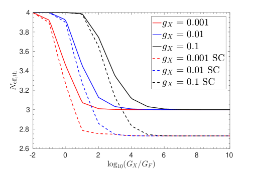
Figure 2: $N_{\mathrm{eff}}$ as a function of effective coupling $G_{X}$. The red, blue and black curves correspond to $g_{X}=$0.001, 0.01, 0.1, respectively. Other parameters are fixed to ${m_{\rm st}}=1~{}{\rm eV}$ and $\sin^{2}\theta_{14}=0.01$, and $\sin^{2}\theta_{24}=0.003$. Full lines correspond to the values obtained with Eq. (2.15) while dashed lines are obtaied under the entropy-conservation-after-decoupling assumption. Eq. (2.16).

2.2 Effects in Big Bang Nucleosynthesis

The $N_{\mathrm{eff}}$ and neutrino number density we have obtained in the previous section have direct effects on the primordial abundances. In the early universe when temperature is much higher than 1 MeV, the primordial plasma consisting of photons, neutrinos, electrons and baryons is in thermal equilibrium with the ratio of the number density of neutrons and protons given by

$$\left(\dfrac{n_{n}}{n_{p}}\right)_{\rm eq}=\left(\dfrac{m_{n}}{m_{p}}\right)^{3/2}e^{-Q_{np}/T}\,,$$ (2.17)

where $Q_{np}=m_{n}-m_{p}=1.3~{}{\rm MeV}$. Because of the small mass difference the neutron-to-proton ratio decreases drastically when the temperature drops below 1 MeV. Neutrons and protons are balanced mainly though beta decay and inverse beta decay, i.e.

$$n+\nu_{e} \leftrightarrow p+e^{-}\,$$

$$n+e^{+} \leftrightarrow p+\bar{\nu}_{e}\,.$$ (2.18)

The two interaction rates are equal and can be approximated by $\Gamma_{np}\propto G_{F}^{2}T^{5}$ provided that $n_{e}=2n_{\nu_{e}}$ since they share the same matrix element. In case neutrino number density deviates from this relation, the neutron-proton conversion rate

$$\Gamma_{np}\propto(1+\rho_{ee})T^{5}\,,$$ (2.19)

At about 1 MeV the relativistic degree of freedom $g_{*}=10.75+\Delta N_{\mathrm{eff}}\,$ where $\Delta N_{\mathrm{eff}}=N_{\mathrm{eff}}-3.046$. In the radiation dominated era, the total energy density $\rho_{\rm tot}\propto g_{*}T^{4}$, and the Hubble rate $H\propto g_{*}^{1/2}T^{2}$. Neutrons freeze out from the plasma when the neutron-proton conversion rate becomes comparable to the the Hubble rate, and we can find the freezing-out temperature

$$T_{f}\propto\left(\dfrac{g_{*}^{1/2}}{1+\rho_{ee}}\right)^{1/3}\,.$$ (2.20)

It shows that both $N_{\mathrm{eff}}$ and electron neutrino number density can affect the time of neutron decoupling. A larger $N_{\mathrm{eff}}$ can increase the expansion rate of the universe, which increases the freezing-out temperature; on the other hand, larger number density of electron neutrinos tend to increase the neutron-proton conversion rate, postponing the time of decoupling. The neutron-to-proton ratio $n_{n}/n_{p}$ is roughly frozen after neutron decoupling until the temperature drops below 0.1 MeV, when the synthesis of nuclei begin. Almost all the remaining neutrons are bounded in the nuclei, thus the neutron-to-proton ratio at decoupling is of crucial importance in the determination of the abundances of primordial elements. We can incorporate the effect of $\nu_{e}$ number density by assuming $\rho_{ee}=1$ but modifying $g_{*}$ to keep $T_{f}$ unchanged. It is straightforward to find the modified $\Delta N_{\mathrm{eff}}$ to be

$$\Delta N_{\mathrm{eff}}^{\prime}=\dfrac{4}{7}\left[\dfrac{43+7\Delta N_{\mathrm{eff}}}{(1+\rho_{ee})^{2}}-10.75\right]\,.$$ (2.21)

This treatment is similar to that of Dolgov et al. [61]. Since $N_{\mathrm{eff}}$ and $\rho_{ee}$ are rather insensitive to the small change in $T_{f}$, while the neutron-to-proton depends on $T_{f}$ exponentially, we use the $N_{\mathrm{eff}}$ and $\rho_{ee}$ at 1 MeV to determine the ratio $n_{n}/n_{p}$.

2.3 $\nu_{s}$ self-interaction in neutrino perturbations

Next we would like to see quantitatively how the new interactions can affect the predictions of CMB and large scale structure (LSS) data. New interactions add collision terms to the Boltzmann equation and make the solution quite complicated. However, it has been shown in Ref. [62] that an exact description of neutrino interactions is quantitatively equivalent to the relaxation time approximation where the collision term can be approximated by [63, 52]

$$\dfrac{1}{f_{0}}\dfrac{\partial f}{\partial\tau}=-\dfrac{\mathcal{N}}{\tau_{\nu}}\,,$$ (2.22)

where $\tau_{\nu}=({a}n_{\nu_{s}}\langle\sigma v\rangle)^{-1}$ is the mean conformal time between collisions and $\mathcal{N}$ is the phase space perturbation of neutrinos. Since $\langle\sigma v\rangle\simeq G_{X}^{2}T_{\nu_{s}}^{2}$, we have

$$\tau_{\nu}^{-1}=\dfrac{3}{2}\dfrac{\zeta(3)}{\pi^{2}}{a}G_{X}^{2}{T_{\nu}^{5}\rho_{ss}}\,,$$ (2.23)

where $\rho_{ss}$ is obtained from the solution of QKEs and $T_{\nu}=\left(\frac{4}{11}\right)^{1/3}T_{\gamma}$ is the neutrino temperature in the standard cosmology .

In the Synchronous gauge, the neutrino Boltzmann equation can be written as

$$\dfrac{\partial\mathcal{N}_{i}}{\partial\tau}+i\dfrac{q}{\epsilon}(\vec{k}\cdot\hat{n})\mathcal{N}_{i}+\dfrac{d\ln f_{0}}{d\ln q}\left[\dot{\eta}-\dfrac{\dot{h}+6\dot{\eta}}{2}(\vec{k}\cdot\hat{n})^{2}\right]=-\Gamma_{ij}\mathcal{N}_{j},.$$ (2.24)

where $i=1,4$ represent the mass eigenstates, $q=ap$ and $\eta$ and $h$ are gravitational potentials (not to be confused with Hubble parameter). $\Gamma_{ij}$ is defined in mass basis as $\Gamma_{ij}=U\mathrm{diag}(0,0,0,1)U^{\dagger}\cdot\tau_{\nu}^{-1}$

We can expand the perturbation $\mathcal{N}$ as in Legendre series [64] and rewrite the Boltzmann equation as (below we denote by “dot” the derivative with respect to proper time)

$$\dot{\mathcal{N}_{i,0}} = -\dfrac{qk}{\epsilon}\mathcal{N}_{i,1}+\dfrac{1}{6}\dot{h}\dfrac{d\ln f_{i,0}}{d\ln q}\,,$$ (2.25)

$$\dot{\mathcal{N}_{i,1}} = \dfrac{qk}{3\epsilon}(\mathcal{N}_{i,0}-2\mathcal{N}_{i,2})\,,$$ (2.26)

$$\dot{\mathcal{N}_{i,2}} = \dfrac{qk}{5\epsilon}(2\mathcal{N}_{i,1}-3\mathcal{N}_{i,3})-(\dfrac{1}{15}\dot{h}+\dfrac{2}{5}\dot{\eta})\dfrac{d\ln f_{i,0}}{d\ln q}-\Gamma_{ij}\mathcal{N}_{j,2}\,,$$ (2.27)

$$\dot{\mathcal{N}_{i,l}} = \dfrac{k}{(2l+1)}\dfrac{q}{\epsilon}\left[l\mathcal{N}_{i,(l-1)}-(l+1)\mathcal{N}_{i,(l+1)}\right]-\Gamma_{ij}\mathcal{N}_{j,l}\,,\quad l\geq 3\,,$$ (2.28)

where $f_{i,0}=f_{\rm FD}\sum_{\alpha}|U_{\alpha i}|^{2}\rho_{\alpha\alpha}$, with $f_{\rm FD}$ a Fermi-Dirac distribution of temperature $T_{\nu}=\left(\frac{4}{11}\right)^{1/3}T_{\gamma}$ for the four neutrinos and again differs from the $f_{0}$ in Ref. [52]. As we mentioned before, this grey body Fermi-Dirac distribution is the assumption of average momentum approximation which yields the most physical $N_{\mathrm{eff}}$ and we restore it here using Eq. (2.6). In order to account for these effects in the analysis of CMB and BAO data we have solved the new collisional Boltzmann equations in a modified version of the Boltzmann code CLASS [65] for an array of values of the model parameters. Furthermore to account for the effects on the background equations we have to include also the modified energy density and pressure of the neutrinos at the starting of the background evolution in CLASS. These are obtained from the solutions of the QKE’s described in the previous section with the average momentum approximation. Under this approximation neutrinos are featured by grey body Fermi-Dirac distributions with normalization factors $\sum_{\alpha}|U_{\alpha i}|^{2}\rho_{\alpha\alpha}$. These distributions are introduced in the CLASS code to infer the background quantities including energy density and pressure

Qualitatively this background effects can be understood in terms of a modification of ${N_{\mathrm{eff}}}$ at CMB times though technically we do not use the variable $N_{\mathrm{eff}}$ when solving the CLASS equations. In any case to help the discussion in what follows we mention an effective $N_{\mathrm{eff}}$ at CMB times, $N_{\mathrm{eff,th}}$, obtained from Eq. (2.15) (or Eq. (2.16) when relevant) for temperatures well below thermalization and well above the non-relativistic transition for the sterile neutrino.

For illustration we plot in Fig. 3 the predicted CMB power spectrum for set of model parameters. For comparison we show in the left panels the results obtained under the assumption of entropy conservation after decoupling employed Ref. [52] while on the right we show our results. In either case, we have set the collision terms to zero in the equations of monopole and dipole to ensure particle number and momentum conservation. In case $\Gamma_{ij}>\cal{H}$, the quadrupole (related to the anisotropic stress of neutrinos) and higher multipoles are suppressed. So in the presence of the interactions the power in higher multipoles are now transferred to the density and velocity fluctuations which in turn contribute to the total gravitational source and enhance the amplitude of the CMB fluctuations that entered the horizon before recombination. This enhancement is clearly seen in the figures when we compare the red line ($G_{X}=10^{7}G_{F}$) with the dashed red line ($G_{X}=10^{10}G_{F}$).

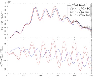
Figure 3: CMB temperature power spectrum. The predicted spectrum in $\Lambda{\rm CDM}$ for the best fit of Planck TT+lowP [37] ($\omega_{b}=0.02222$, $\omega_{\rm cdm}=0.1197$, $H_{0}=67.31{\rm km}{\rm s}^{-1}{\rm Mpc}^{-1}$, $\tau_{\rm reio}=0.078$, $\ln 10^{10}A_{s}=3.089$, and $n_{s}=0.9655$) (i.e. the size of the sound horizon at recombination $100\theta_{\rm MC}$ has been adjusted to fix $H_{0}=67.31{\rm km}{\rm s}^{-1}{\rm Mpc}^{-1}$ in these curves, and this is so to illustrate the effect of new interaction on the size of the sound horizon) is shown in black along with error bars from Planck 2015 data. Colored lines correspond to $\Lambda{\rm CDM}$ models with one sterile neutrino species and new interactions. Cosmological parameters are the same as the best fit of Planck TT+lowP and the implicit parameters for new interactions are the same as Fig. 1 ($g_{X}=0.1$, ${m_{\rm st}}=1~{}{\rm eV}$, and $\sin\theta_{14}=0.1$). In the left panels the results are obtained under the assumption of entropy conservation after decoupling employed Ref. [52] while in the right we show our results. The solid blue, solid red and dashed red lines show different interaction strength corresponding to $G_{X}=10^{-2}G_{F}\,(N_{\mathrm{eff,th}}=4$ in both left and right panels), $G_{X}=10^{7}G_{F}\,$ (i.e. $N_{\mathrm{eff,th}}=2.7$ in the left panel while $N_{\mathrm{eff,th}}=3$ in the right), $G_{X}=10^{10}G_{F}$ (i.e. $N_{\mathrm{eff,th}}=2.7$ in the left panel while $N_{\mathrm{eff,th}}=3$ in the right), respectively. The lower panel displays the relative difference between models with different interaction strength and the best-fit $\Lambda{\rm CDM}$ model.

We also notice that the location of the peaks is shifted in the new interaction models compared with the $\Lambda{\rm CDM}$ best fit. This is the effect associated with the modification of the neutrino background phase space distributions and can be understood qualitatively as the modification of $N_{\mathrm{eff}}$ and it is therefore most different between the right and left panels. For models with strong self-interactions for which at the CMB times $N_{\mathrm{eff}}<N_{\mathrm{eff,th}}\leq 3\;(2.7)$ in the right (left) panels, and the peaks move to the left as expected from the earlier time of mater-radiation equality ($N_{\mathrm{eff}}<N_{\mathrm{eff,th}}$ because for CMB observables the contribution of the sterile neutrino to the radiation energy density is further reduced because they become partially non-relativistic during recombination). The shift is consequently more pronounced for the panels on the left. The solid blue line ($G_{X}=10^{-2}G_{F}$), on the other hand, shows the opposite behaviour since for these weak interactions the resulting $N_{\mathrm{eff}}$ is always larger than 3. Indeed, as a cross check, we have verified explicitly that the blue line can exactly mimic the behavior of a sterile species without interactions. The new interaction in this case is too weak to be significant in the thermalization of sterile neutrinos.

3 Data analysis: results

In this section we show the results of confronting the sterile self-interaction model with BBN, CMB and BAO data. Technically to obtain the predictions for these observables as a function of the model parameters we interface the solutions of QKEs with MultiNest [66, 67, 68] or with the modified CLASS by interpolating the tabulated solutions in the model parameter space and feed them to the codes.

Our aim is to explore as large model parameter space as possible but solving the QKEs and running CLASS is time demanding. So as a compromise, we allow the parameters to vary within the range $G_{X}=10^{-2}G_{F}\sim 10^{10}G_{F}$ (from much smaller than weak coupling to much larger than weak coupling), $g_{X}=10^{-3}\sim 10^{-1}$ (so we treat the gauge boson mass $M_{X}$ as a parameter derived from $G_{X}$ and $g_{X}$ and within the chosen ranges for these parameters it varies between 1 keV$\lesssim M_{X}\lesssim 120$ GeV). As for the sterile mass parameters we allow ${m_{\rm st}}^{2}=0.01~{}{\rm eV}^{2}\sim 10~{}{\rm eV}^{2}$ so that the allowed sterile neutrino mass can be as low as the 95% CL of the cosmological bounds on neutrino masses, and can be much larger than the mass suggested by short baseline anomalies. The sterile neutrino mixing angles $\sin^{2}\theta_{14}$ is varied in a range as large as $0.003\sim 0.3$ motivated by the latest analysis of the SBL electron neutrino disappearance data [35]. In view of the tension between the between SBL $\nu_{e}$ appearance channel and $\nu_{\mu}$ results we chose $\sin^{2}\theta_{24}$ to be compatible with the bounds from $\nu_{\mu}$ disappearance. In order to keep the fit manageable we fix it to be 30% of $\sin^{2}\theta_{14}$. Finally with the existing oscillation data it is challenging to constrain the mixing between tau neutrinos and sterile states. So for simplicity we just assume $\sin\theta_{34}=0$. As we will see later, our results do not depend on a particular choice of mixing parameters.

3.1 BBN

Let us discuss first the results obtained from the analysis of BBN abundances of ${}^{4}{\rm He}$ and deuterium. They have been determined by observations to be [69]

$$Y_{\rm P}\equiv 4\dfrac{n_{\rm He}}{n_{b}}=0.2465\pm 0.0097\,,$$ (3.1)

and [70]

$$y_{\rm DP}\equiv 10^{5}\dfrac{n_{\rm D}}{n_{\rm H}}=2.53\pm 0.04\,,$$ (3.2)

where $n_{b}$, $n_{\rm He}$, $n_{\rm D}$, $n_{\rm H}$ are the number density of baryons and helium, deuterium and hydrogen nuclei respectively. To allow for a faster confrontation of the model predictions with BBN data, we use the predicted helium and deuterium abundances given by Taylor expansions obtained with the PArthENoPE code [71], i.e.

$$Y_{\rm P} = 0.2311+0.9502\omega_{b}-11.27\omega_{b}^{2}$$ (3.3)

$$+ \Delta N_{\mathrm{eff}}^{\prime}(0.01356+0.008581\omega_{b}-0.1810\omega_{b}^{2})$$

$$+ \Delta N_{\mathrm{eff}}^{\prime 2}(-0.0009795-0.001370\omega_{b}+0.01746\omega_{b}^{2})\,,$$

$$y_{\rm DP} = 18.754-1534.4\omega_{b}+48656\omega_{b}^{2}-552670\omega_{b}^{3}$$ (3.4)

$$+ \Delta N_{\mathrm{eff}}^{\prime}(2.4914-208.11\omega_{b}+6760.9\omega_{b}^{2}-78007\omega_{b}^{3})$$

$$+ \Delta N_{\mathrm{eff}}^{\prime 2}(0.012907-1.3653\omega_{b}+37.388\omega_{b}^{2}-267.78\omega_{b}^{3})\,,$$

where $\omega_{b}$ is the energy density of baryons today defined as $\omega_{b}\equiv\Omega_{b}h^{2}$ and $h\equiv H_{0}/(100{\rm kms^{-1}Mpc^{-1}})$. The treatment is similar to that of Planck Collaboration [37]. These theoretical predictions are subject to errors from neutron lifetime and the interaction rate of ${\rm d(p,}\gamma)^{3}{\rm He}$ of the order of $\sigma^{\rm th}(Y_{\rm P})=0.0003$ and $\sigma^{\rm th}(y_{\rm DP})=0.06$. Since these theoretical errors are not correlated with the errors from observations, we can add them in quadrature.

With these data we construct the likelihood

$$-2\ln{\cal L}(\vec{\omega})=\dfrac{(Y_{\rm P}(\vec{\omega})-Y_{\rm P}^{\rm dat})^{2}}{(\sigma^{\rm dat}_{Y_{\rm P}})^{2}+(\sigma^{\rm th}_{Y_{\rm P}})^{2}}+\dfrac{(y_{\rm DP}(\vec{\omega})-y_{\rm DP}^{\rm dat})^{2}}{(\sigma^{\rm dat}_{y_{\rm DP}})^{2}+(\sigma^{\rm th}_{y_{\rm DP}})^{2}}\,,$$ (3.5)

where the relevant model parameters are $\vec{\omega}=(G_{X},g_{X},\omega_{b},{m_{\rm st}},\sin^{2}\theta_{14})$ and use MultiNest [66, 67, 68] as a Bayesian inference tool.

We assume flat priors on $\log G_{X}$, $g_{X}$ and $\omega_{b}$ within the range $-2\leq\log_{10}(G_{X}/G_{F})\leq 10\,$, $0.001\leq g_{X}\leq 0.1\,$, and $0.02153\leq\omega_{b}\leq 0.02291\,$, where the prior on $\omega_{b}$ is the 3$\sigma$ range as obtained from Ref. [37]. We also assume gaussian priors on and ${m_{\rm st}}$ and $\sin^{2}\theta_{14}$ with ${m_{\rm st}}=1.13\pm 0.02~{}{\rm eV}$ and $\sin^{2}\theta_{14}=0.009\pm 0.003$ as motivated by the fit of $\nu_{e}$ disappearance data in Ref [35]. We show for comparison the results obtained also under the SC assumption of Eq. (2.16) as dashed lines in the upper left and lower right panels and void regions in the lower left panel. The results are shown in Fig. 4.

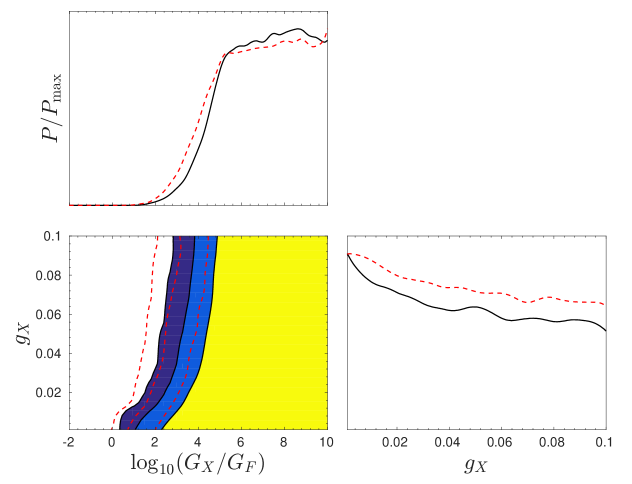
Figure 4: Posteriors of $\log_{10}(G_{X}/G_{F})$ and $g_{X}$ from the fit to the BBN abundances of ${}^{4}{\rm He}$ and deuterium. The yellow, blue and dark blue regions correspond to the $2\sigma$, $3\sigma$ and $4\sigma$ allowed ranges, respectively. We show for comparison the results obtained under the SC assumption of Eq. (2.16) as dashed red lines in the upper left and lower right panels and void regions in the lower left panel with dashed boundaries representing the corresponding $2\sigma$, $3\sigma$ and $4\sigma$ allowed ranges, respectively.

As expected very small $G_{X}$ is disfavored since it yields $N_{\mathrm{eff}}$ close to 4. Conversely the posterior distribution of $g_{X}$ is almost flat meaning this parameter is very mildly constrained by BBN data within the chosen range. Allowed ranges for the parameters are $g_{X}\leq 0.065\,(1\sigma)$ and $g_{X}\leq 0.095\,(2\sigma)$ , and $\log_{10}(G_{X}/G_{F})\geq 6.1\,(1\sigma)$ and $\log_{10}(G_{X}/G_{F})\geq 4.0\,(2\sigma)$. As seen in the figure if one had obtained $N_{\mathrm{eff}}$ under the assumption of entropy conservation after decoupling, the lower bounds on $\log_{10}(G_{X}/G_{F})$ would have been somewhat weaker while the allowed range of $g_{X}$ would be almost the same.

3.2 CMB and BAO

Most sensitivity to the sterile self-interacting model can be derived from the analysis of the CMB and BAO data. For concretness we include in the analysis the CMB spectrum from Planck 2015 [72] high multipole temperature correlation data as well as the low multipole polarization data (denoted as “Planck TT+lowP” in Planck’s publications, and we use “TT” here for short). We also include the measurements of the scale of the baryon acoustic oscillation (BAO) peaks at different red shifts as measured in the 6dF Galaxy Survey [73], the SDSS DR7 main Galaxy samples [74], the CMASS [75] and LOWZ [76] samples from SDSS DR11 results of BOSS experiment.

To do the analysis we interface the output of the QKEs with the modified CLASS code for the neutrino Boltzmann equations and use Markov Chain Monte Carlo (MCMC) code Monte Python [77] for parameter inference. In total we have 10 parameters in this study. The six cosmological parameters are the same as the base $\Lambda{\rm CDM}$ model in Ref. [37], i.e. the baryon energy density $\omega_{b}\equiv\Omega_{\rm b}h^{2}$, the cold dark matter density $\omega_{\rm cdm}\equiv\Omega_{\rm cdm}h^{2}$, the size of sound horizon at recombination $100\theta_{\rm MC}$, the optical depth to reionisation $\tau_{\rm reio}$ and the amplitude and tilt of the initial power spectrum $\ln(10^{10}A_{s})$ and $n_{s}$ respectively. All six cosmological parameters have flat priors without upper nor lower limits except $\tau_{\rm reio}\geq 0.04$. Besides the six cosmological parameters, we have the four model parameters to describe the new scenario: $\log_{10}(G_{X}/G_{F})$, $g_{X}$, ${m_{\rm st}}$ and $\sin^{2}\theta_{14}$. Their prior ranges can be found in Table 1. We also fix the sum of the neutrino masses of active states to be 0.06 eV.

Prior	$\log_{10}(G_{X}/G_{F})$	$g_{X}$	${m_{\rm st}}({\rm eV})$	$\sin^{2}\theta_{14}$
Broad	$[-2,\,10]$	$[0.001,\,0.065]$	$[0.1,\,3]$	$[0.003\,,0.3]$
Narrow	$[-2,\,10]$	$[0.001,\,0.065]$	$1.13\pm 0.02$	$0.009\pm 0.003$

Table 1: Prior ranges for “broad prior” and “narrow prior”. All the parameters are flat except ${m_{\rm st}}$ and $\sin^{2}\theta_{14}$ for narrow prior which are instead gaussian with the center and width listed above.

As seen in the table we impose two different priors on ${m_{\rm st}}$ and $\sin^{2}\theta_{14}$. One is flat in the range $0.1~{}{\rm eV}\leq{m_{\rm st}}\leq 3~{}{\rm eV}$ and $0.003\leq\sin^{2}\theta_{14}\leq 0.3$, which we denote as “broad prior”. It was chosen with the aim at studying the information on these parameters which can be derived from cosmology in the presence of self-interacting scenario . The other one is gaussian with ${m_{\rm st}}=1.13\pm 0.02~{}{\rm eV}$ and $\sin^{2}\theta_{14}=0.009\pm 0.003$ and is the same as the one we have adopted for the BBN analysis and it aims at targeting specifically the SBL anomaly. We denote it as “narrow prior”. Technically, the narrow prior is imposed by adding a gaussian likelihood to the data likelihood.

The prior of the parameter $g_{X}$ is flat in the limited range $[0.001,\,0.065]$ as motivated by the $1\sigma$ range of BBN constraint discussed above. We notice that $g_{X}$ only enters in the CMB and BAO observables indirectly via its effect on the modified energy density and pressure of the neutrinos at the starting of the background evolution in CLASS. We have verified that extending its range would not add more freedom to the analysis while it affects numerical convergence.

As stressed above, in the analysis of CMB and BAO data $N_{\mathrm{eff}}$ is never used as an input. Still, for a given value of model parameters we can obtain the value of $N_{\mathrm{eff}}$ at the relevant temperatures. In this way, given the priors for the four model parameters we can infer the corresponding prior for $N_{\mathrm{eff}}$ This is shown in Fig. 5 where we plot the derived priors of $N_{\mathrm{eff,th}}$ corresponding to the two model priors for the relevant parameters. As $N_{\mathrm{eff,th}}$ mainly depends on the effective coupling $G_{X}$, if $G_{X}\gg G_{F}$, $N_{\mathrm{eff,th}}\simeq 3$; on the other hand, if $G_{X}\ll G_{F}$, $N_{\mathrm{eff,th}}\simeq 4$. Therefore the resultant $N_{\mathrm{eff,th}}$ of both broad and narrow priors is peaked at these two extremes and it differs from those extreme values in a very small range of the input parameter space. In the figure we also include a modified prior which is nearly flat in $N_{\mathrm{eff}}$ that we comment upon in the Appendix. Let us mention that if one uses the assumption of entropy conservation after decoupling in the evaluation of $N_{\mathrm{eff}}$ the prior would be similar in shape but the low peak would be at $N_{\mathrm{eff,th}}=2.7$.

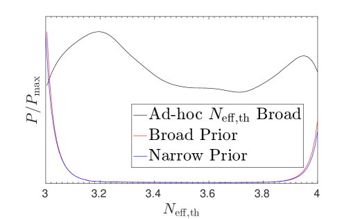
Figure 5: Resulting priors on $N_{\mathrm{eff,th}}$ for broad prior (red line) and narrow prior (blue line). For comparison we also and add-hoc prior in which we cut the parameter space of $M_{X}$ to force a nearly flat prior on $N_{\mathrm{eff,th}}$. See Appendix A.1 for details.

We have summarized the results of our analysis in Table 2 and Fig. 6 where we give the allowed ranges of the 6+4 parameters and the posterior probability distribution for the four sterile model parameters respectively. As expected there is nearly no constraint on $g_{X}$ and $\sin^{2}\theta_{14}$. The 95% CL limit on ${m_{\rm st}}$ for broad prior and TT data is ${m_{\rm st}}<0.95~{}{\rm eV}$ . It can be compared with the 95% limit of ${m_{\rm st}}<0.82~{}{\rm eV}$ in terms of the S$\Lambda{\rm CDM}$ model in Ref. [52]. As expected when dropping the assumption of entropy conservation after decoupling the limit is slightly relaxed. But, still, even in the presence of self-interactions with a wide range of couplings a sterile neutrino with mass larger than $1~{}{\rm eV}$ is excluded by more than $2\sigma$. Adding BAO data puts even tighter constraint on ${m_{\rm st}}$ and we find ${m_{\rm st}}<0.37~{}{\rm eV}$ at 95% CL.

	Broad Prior		Narrow Prior
Parameter	TT	TT+BAO	TT	TT+BAO
$\omega_{b}$	$0.02209^{+0.00022}_{-0.00026}$	$0.02242^{+0.00021}_{-0.00027}$	$0.02204\pm 0.00024$	$0.02282^{+0.00026}_{-0.00030}$
$\omega_{\rm cdm}$	$0.1201\pm 0.0022$	$0.1182^{+0.0012}_{-0.0037}$	$0.1200^{+0.0022}_{-0.0025}$	$0.1150^{+0.0025}_{-0.0034}$
$100\theta_{\rm MC}$	$1.04187\pm 0.00047$	$1.04200^{+0.00060}_{-0.00043}$	$1.04189^{+0.00047}_{-0.00056}$	$1.04220^{+0.00058}_{-0.00055}$
$\ln 10^{10}A_{s}$	$3.093^{+0.033}_{-0.041}$	$3.116\pm 0.041$	$3.095\pm 0.037$	$3.170^{+0.041}_{-0.046}$
$n_{s}$	$0.9592\pm 0.0084$	$0.941^{+0.005}_{-0.010}$	$0.9499\pm 0.0078$	$0.9822^{+0.0073}_{-0.012}$
$\tau_{\rm reio}$	$0.080^{+0.017}_{-0.020}$	$0.093\pm 0.020$	$0.081\pm 0.019$	$0.123\pm 0.020$
$\log_{10}(G_{X}/G_{F})$	$[1.46,8.90]$	$[-0.03,8.30]$	$[1.74,9.45]$	$[-0.55,5.32]$
$g_{X}$	-	-	-	$<0.041$
${m_{\rm st}}/{\rm eV}$	$<0.95$	$<0.37$	$1.12\pm 0.02$	$1.12\pm 0.02$
$\sin^{2}\theta_{14}$	-	-	$0.009\pm 0.003$	$0.009\pm 0.003$
$H_{0}$	$64.9^{+1.8}_{-1.6}$	$68.16^{+0.58}_{-1.5}$	$61.97^{+0.90}_{-1.1}$	$67.4^{+1.0}_{-1.5}$
$N_{\mathrm{eff}}$	$<3.21$	-	$<3.23$	-

Table 2: Allowed ranges for the model parameters for different priors and data sets. Cosmological parameters are shown in mean$\pm 1\sigma$ and the parameters for the new interaction are shown in 95% CL except for ${m_{\rm st}}$ and $\sin^{2}\theta_{14}$ in narrow priors. In entries marked as $-$ the full prior range is allowed. We also show the corresponding derived ranges for $H_{0}$ in unit of ${\rm km}{\rm s}^{-1}{\rm Mpc}^{-1}$.

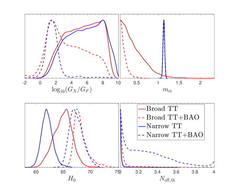
Figure 6: Posterior distribution of relevant cosmological and new interaction parameters. The solid red, dashed red, solid blue and dashed blue lines correspond to broad prior with Planck data, broad prior with Planck+BAO data, narrow prior with Planck data and narrow prior with Planck+BAO data, respectively. They are normalized so that the maximum probability density is 1. We stress that both $N_{\mathrm{eff,th}}$ and $H_{0}$ are derived parameters.

We also notice that the interacting $\nu_{s}$ scenario with large $G_{X}$ ($G_{X}>10^{4}G_{F}$) is preferred over the non-interacting scenario when considering TT data only. This is expected since small $G_{X}$ tends to produce $N_{\mathrm{eff}}\simeq 4$ which is too far away from the favoured value of 3 to be reconciled with the shift of other cosmological parameters. What is more surprising is that by adding BAO data, the favouring of large $G_{X}$ drops significantly while that of small $G_{X}$ is lifted.

To better understand this behaviour we plot in Fig. 7 the predicted values of the BAO observable

$$D_{V}(z)=\left[(1+z)^{2}D_{A}^{2}(z)\dfrac{cz}{H(z)}\right]^{1/3}\,,$$ (3.6)

as a function of redshift. $D_{A}(z)$ is the angular diameter distance, $H(z)$Hubble parameter and $r_{s}$ is the comoving sound horizon at the end of the baryon drag epoch.

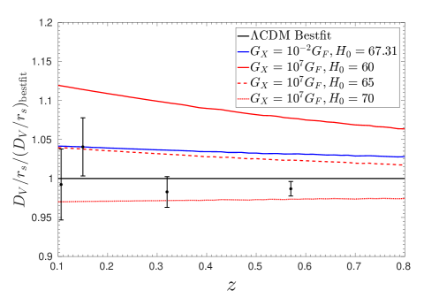
Figure 7: $D_{V}/r_{s}$ as a function of redshift $z$ normalized to the $\Lambda{\rm CDM}$ prediction (for the same parameters as Fig. 3 for which $H_{0}=67.31~{}{\rm km}{\rm s}^{-1}{\rm Mpc}^{-1}$). BAO data and error bars are shown in black. The colored lines correspond to the interacting $\nu_{s}$ scenario with $g_{X}=0.1$, ${m_{\rm st}}=1~{}{\rm eV}$, and $\sin\theta_{14}=0.1$ and different values of $G_{X}$ as labeled in the figure. For these curves the other cosmological parameters have been fixed to the $\Lambda{\rm CDM}$ best fit except the size of the sound horizon at recombination $100\theta_{\rm MC}$ which has been adjusted to produce the corresponding values of $H_{0}$ given in the label (in units of ${\rm km}{\rm s}^{-1}{\rm Mpc}^{-1}$).

Let us stress that in our numerical analysis so far we have used as input parameters the ten parameters described above, so given a set of values for the ten parameters, $H_{0}$ is a derived quantity. For example for the parameters at the best fit of $\Lambda{\rm CDM}$ the Hubble constant comes out to be $H_{0}=67.31\,{\rm km}{\rm s}^{-1}{\rm Mpc}^{-1}$. But when showing the predictions in Fig. 7 to better control the dependence on $H_{0}$ we have traded one of the input parameters, $100\theta_{\rm MC}$ by $H_{0}$. By fixing $\omega_{b}$ and $\omega_{\rm cdm}$, $r_{s}$ is more or less fixed. But a change in $H_{0}$ modifies the fraction of dark energy, which changes the comoving distance back to the baryon drag epoch. Because of this $D_{V}$ is also modified. And as we can see from Fig. 7 for the strong interacting scenario BAO data favours $H_{0}$ in between 65 ${\rm km}s^{-1}{\rm Mpc}^{-1}$ and 70 ${\rm km}s^{-1}{\rm Mpc}^{-1}$. Indeed, we see that the prediction for a strongly interacting $\nu_{s}$ but with $H_{0}$ as low as 60 ${\rm km}{\rm s}^{-1}{\rm Mpc}^{-1}$ is even worse than the case of non-interacting sterile neutrinos with $H_{0}=67.31~{}{\rm km}{\rm s}^{-1}{\rm Mpc}^{-1}$. The tension cannot be accommodated by varying other cosmological parameters in the range allowed by CMB data.

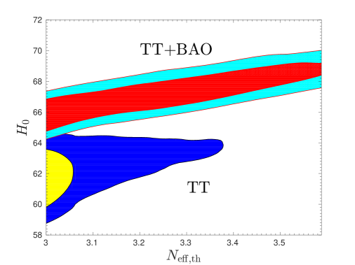
Figure 8: 2-dimensional posterior correlation of $H_{0}$ and $N_{\mathrm{eff,th}}$ for the narrow prior case. The yellow and blue regions show the 68% and 95% credible intervals using Planck data only. The red and cyan regions are the corresponding ones using Planck+BAO data.

However, a small $H_{0}$ is preferred by TT data, as we can see from Table 2 and Fig. 6. For example when using the broad (narrow) prior we find that TT data prefers $H_{0}=64.9^{+1.8}_{-1.6}~{}{\rm km}{\rm s}^{-1}{\rm Mpc}^{-1}$ ($H_{0}=61.97^{+0.90}_{-1.1}~{}{\rm km}{\rm s}^{-1}{\rm Mpc}^{-1}$) It is known that there exists a strong correlation between $H_{0}$ and $N_{\mathrm{eff}}$ which we have shown in Fig. 8 by plotting the two-dimensional posterior allowed regions for those parameters from the analysis with narrow prior (the corresponding ones for the broad prior are not very different). Thus the change in $N_{\mathrm{eff}}$ has to be compensated by the shift in $H_{0}$ which explains the small $H_{0}$ favored by Planck data. However this small $H_{0}$ raises a tension with the BAO data. So when adding BAO to the analysis, a small $G_{X}$ which predicts large $N_{\mathrm{eff}}$ and large $H_{0}$ may give a better (if still bad) overall description. Let us comment in passing that this tension would have been even worse if one have used the assumption of entropy conservation after neutrino decoupling to the point that the non-interacting scenario with one fully thermalized sterile neutrino would give a better fit to TT+BAO than the strongly interacting case.

The previous discussion leads us to the question of whether the addition of sterile neutrino self-interactions does indeed help to reconcile eV sterile neutrinos with cosmological observations. To address this question we have summarized in Table 3 the minimum $\chi^{2}$ obtained in the full parameter space explored for the different analysis.

Data	$\Lambda{\rm CDM}$	Free-$\nu_{s}$ BP	Free-$\nu_{s}$ NP	Int-$\nu_{s}$ BP	Int-$\nu_{s}$ NP
TT	11261.9	9.0	18.5	1.7	6.4
TT+BAO	11266.4	7.3	32.0	1.1	22.1

Table 3: $\chi^{2}_{\rm min}$ for various models and data combinations. The first column show the minimum of $\Lambda{\rm CDM}$ model (this $\chi^{2}_{\rm min}$ is obtained from the chains of Planck Collaboration available at http://irsa.ipac.caltech.edu/data/Planck/release_2/ancillary-data/.), and others display the shift $\chi^{2}_{\rm min}$ with respect to this $\Lambda{\rm CDM}$ value. “Free-$\nu_{s}$ BP” and “Free-$\nu_{s}$ NP” are models of $\Lambda{\rm CDM}$ with one non-interacting sterile neutrino species with ${m_{\rm st}}$ and $\theta_{14}$ priors as in Table 1 but with a fixed and very weak interaction ($G_{X}=10^{-2}G_{F}$ so effectively for this model $N_{\mathrm{eff}}=4$).

From the table we read that the best fit for the interacting $\nu_{s}$ model with the broad priors is always comparable to the $\Lambda{\rm CDM}$ best fit, and much better than the case without new interactions. This is because within the broad prior there always exists an interaction strength which predicts $N_{\mathrm{eff}}\simeq 3$ and a reasonable fit can be obtained at the lower limit of the allowed range of ${m_{\rm st}}$.

For the interacting $\nu_{s}$ model with narrow priors we find that, as for cosmological data respects, $\Lambda{\rm CDM}$ is a better fit by $\Delta\chi^{2}_{\rm min}=-6.4$ when using TT data, but still, it provides a much better description than the non-interacting case. However, as read from the table, including BAO data (which are 4 data points) increases the $\chi^{2}$ of both interacting and non-interacting scenarios with the narrow prior by $\sim$ 15 units as a consequence of the tension between the $H_{0}$ values favoured by CMB and BAO in this scenario. Therefore we conclude that self-interactions of $\nu_{s}$ have limited power to reconcile the sterile neutrinos required by the short baseline anomalies when the BAO information is included.

4 Conclusions

In this work we have revisited the scenario with self-interaction among light sterile neutrinos mediated by a massive gauge boson proposed to alleviate the tension between ${\cal O}$(eV) sterile neutrinos – motivated by the SBL anomalies–, and the cosmological bounds on the presence of extra radiation and neutrino masses. We have explored a wide range of the model parameters with the goal of determining if such secret interaction can (or cannot) improve the description of cosmological data.

For each point in the model parameter space we have obtained the effective number of neutrino species at the time of BBN by solving the QKEs quantifying the neutrino flavour evolution. Subsequently we have consistently introduced these results in the evolution of the density perturbations relevant for predicting the CMB and BAO data. In order to do so we have solved the modified collisional Boltzmann equations for the perturbations accounting also for the effects of the modified energy density and pressure of the neutrinos in the background evolution.

With these predictions we have first performed an analysis of the BBN data in terms of the primordial abundances of ⁴He and deuterium which mostly yelds information on the the effective interaction strength which we find to be bounded to $\log_{10}(G_{X}/G_{F})\geq 4.0$ at 95% CL. We have then performed a Bayesian analysis of CMB and BAO measurements for two different priors on the sterile neutrino mass and mixings. By allowing a wide prior for the sterile neutrino mass, we find ${m_{\rm st}}\leq 0.95~{}{\rm eV}$ (95% CL) considering Planck data only and ${m_{\rm st}}\leq 0.37~{}{\rm eV}$ (95% CL) using a combination of Planck and BAO data. So the mass bounds are slightly relaxed compared with that of a non-interacting sterile neutrino model but a sterile neutrino mass of 1 eV is still excluded by more than $2\sigma$ CL. We also performed an analysis by fixing the sterile neutrino mass and mixing to the values preferred by short baseline data. Both analysis show that Planck data alone favors relatively large $G_{X}$, i.e. the new interaction scenario, while including BAO information significantly increases the probability of models with small $G_{X}$, i.e the non-interacting scenario. We have shown how this can be explained by the known degeneracy between $H_{0}$ and $N_{\mathrm{eff}}$— the small $N_{\mathrm{eff}}$ leads to small $H_{0}$, which is in contradiction with the BAO data. As a consequence the overall quality of the fit is severely degraded. Furthermore this is also at odds with the lower bound on the interaction strength implied by BBN.

We conclude then that adding the new interaction can alleviate the tension between eV sterile neutrinos and Planck data, but when including also the BAO results, the self-interacting sterile neutrino model cannot provide a consistent global description of the cosmological observations.

Appendix A Appendix

A.1 Dependence on the derived prior of $N_{\mathrm{eff}}$

The priors for the model parameters used in our analysis lead to a derived prior for $N_{\mathrm{eff}}$ which is highly peak at either 3 or 4 as shown in Fig. 5 and while TT favours models close to the 3 peak, BAO disfavours them especially in the narrow prior case. One may wonder then if for models leading to $N_{\mathrm{eff}}$ in the intermediate region one could find some compromise. This possibility however is not observed in the posterior distribution of those analysis as a result of the “volume effect” of the priors.

It is important to stress however that the conclusion about the bad quality of the overall description of the TT+BAO data when using the narrow prior holds independently of this prior bias because it is based on the value of the minimum $\chi^{2}$ of the analysis which is independent of the shape of prior probability distributions.

Still, to quantify the effect of the bias induced by the model priors in the derived posterior for the broad prior analysis, we have searched for an add-hoc prior for the four model parameters which resulted into a derived prior for $N_{\mathrm{eff}}$ which was as flat as possible. We found that for this it was best to use $M_{X}$ and $g_{X}$ as base parameters instead of $G_{X}$ and $g_{X}$. With a flat prior on $\log_{10}M_{X}$ for $M_{X}$ between 40 MeV and 1200 MeV and $g_{X}$ still flat between 0.001 and 0.065 (so the derived range of $-2\leq\log_{10}(G_{X}/G_{F})\leq 4.6$) and with broad or narrow prior ranges for ${m_{\rm st}}$ and $\theta_{14}$, the derived $N_{\mathrm{eff}}$ prior obtained is that shown in the corresponding curve in Fig. 5, which, as seen in the figure, is relatively flat between 3 and 4.

The resulting posterior for ${m_{\rm st}}$ and $N_{\mathrm{eff}}$ for the analysis with this add-hoc broad prior are shown in Fig. 9.

Figure 9: Posterior distribution of ${m_{\rm st}}$ and $N_{\mathrm{eff}}$ assuming the add-hoc $N_{\mathrm{eff}}$ prior and for the data combinations as labeled in the figure.

The first thing we notice is that with the ad-hoc prior we do not observe the long tale in the $N_{\mathrm{eff,th}}$ probability distribution for the narrow prior observed in Fig. 6 (and with a non-negleable probability for the non-interacting case $N_{\mathrm{eff}}=4$) when including BAO data. We find instead that even when considering TT+BAO data $N_{\mathrm{eff}}<3.41$ and ${m_{\rm st}}<0.37~{}{\rm eV}$ at 95% CL. In what respects to the interaction parameters for the add-hoc prior we find that the full range of $g_{X}$ is allowed at this CL while $40\leq M_{X}\leq 840$ MeV when using TT data only (which implies $0.57\leq\log_{10}(G_{X}/G_{F})\leq 4.4$) while the range of $70\leq M_{X}\leq 1000$ MeV and $0.47\leq\log_{10}(G_{X}/G_{F})\leq 4.1$ is allowed in the TT+BAO analysis.

We finish by commenting that when using this ad-hoc quasi-flat $N_{\mathrm{eff}}$ prior we can cross-check the results of our analysis with the corresponding analysis performed by the Planck collaboration in terms of an “effective” sterile neutrino mass with free $N_{\mathrm{eff}}$  [37]. We find that our results are consistent with those obtained by Planck collaboration in their analysis (which includes TT+lensing+BAO data) $N_{\mathrm{eff}}<3.7$ and $m^{\rm eff}_{\nu,{\rm sterile}}<0.38~{}{\rm eV}$.

A.2 Validity of $T_{\nu}<M_{X}$ approximation

We have performed our analysis in a relatively broad range of $G_{X}$ and $g_{X}$. They correspond to the gauge boson mass in a range as large as 120 GeV and as small as 1 keV. However when solving the QKEs we always assume $T_{\nu}<M_{X}$ so that the Lagrangian can be approximated by $4\nu$ effective interaction. One may question if the approximation is still valid for small $M_{X}$.

To estimate the parameter region in which our approximation is not valid we look for the parameters for which more than 50% of the sterile neutrinos are produced at $T_{\nu}>M_{X}$. Technically we require $\rho_{ss}$ not to have reached 0.5 when neutrino temperature drops below $M_{X}$. We show in the left panel of Fig. 10 the inconsistent region of $G_{X}$ and $g_{X}$ while allowing mixing angle and ${m_{\rm st}}$ to vary within the solution limits. In other words, this is the maximum inconsistent region for $G_{X}$ and $g_{X}$. Recalling the definition of $G_{X}$ ($\frac{G_{X}}{\sqrt{2}}=\frac{g_{X}^{2}}{8M_{X}^{2}}$), the boundary line of the region corresponds to a constant $M_{X}\simeq 64~{}{\rm keV}$. Inside the region $M_{X}$ is smaller than this value.

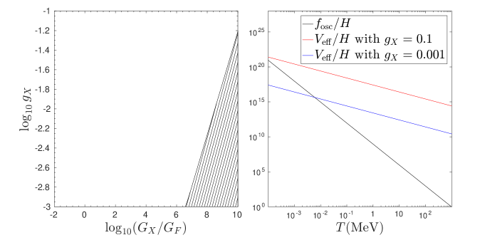
Figure 10: Left: Maximum inconsistent region obtained by adding up the inconsistent region of all allowed mixing angle and sterile neutrino mass. The hatched region may not be well consistent with the four-fermion approximation we have adopted in this work. Right: The effective potential and oscillation frequency as a function of the photon temperature for $g_{X}=0.1$ (red line) and $g_{X}=0.001$ (blue line). We assume $T_{\nu}=(\frac{4}{11})^{1/3}T_{\gamma}$ and ${m_{\rm st}}=1~{}{\rm eV}$.

From the solutions of QKEs we find that for all the parameters in the inconsistent region we always obtain $N_{\mathrm{eff}}\simeq 3$, regardless of the choice of ${m_{\rm st}}$ and $\sin^{2}\theta_{14}$. We argue next that despite the approximation does not hold, the solution obtained is still valid.

To qualitatively confirm this, we look at what would be the effective potential in case $T_{\nu}>M_{X}$ where ${V_{\rm eff}}\simeq\frac{g_{X}^{2}T_{\nu}^{2}}{8E}$ [50] and compare it with the oscillation frequency and the Hubble parameter. This is shown in the right panel of Fig. 10 (as a qualitative estimate we average $1/E$ over the phase space distribution of neutrinos and replace it by $0.456T_{\nu}$ in the plotted ${V_{\rm eff}}$). As seen in the figure, in the full range of $g_{X}$ we use, the effective potential is always much larger than the oscillation frequency for temperatures above 1 MeV. This again leads to the suppression of the in-medium mixing angle in Eq. 2.3 and the late production of sterile neutrinos which leads to $N_{\mathrm{eff}}\simeq 3$. Notice that the maximum $M_{X}$ of 64 keV is much smaller than 1 MeV so for these curves it is always the case that $T_{\nu}>M_{X}$ We conclude that our solutions do still hold even in the region where $T_{\nu}<M_{X}$ approximation fails.

One caveat of the above argument is the possible effects associated with the direct production of the massive gauge boson if light enough. In the region of parameters we consider this is only expected to happen well after neutrino decoupling and therefore cannot lead to an increase of $N_{\mathrm{eff}}$. As a matter of fact, a massive gauge boson model in the $T_{\nu}\gg M_{X}$ limit is qualitatively equivalent to the massless pseudoscalar model discussed in Ref. [48] where the QKEs describing two-neutrino oscillation shows $g_{X}$ has to be smaller than $10^{-5}$ to achieve $N_{\mathrm{eff}}>3$. This tells us that in our parameter range, the condition $T_{\nu}\gg M_{X}$ implies that the thermalizaiton between active and sterile neutrinos has never happened. In other words in our scenario $N_{\mathrm{eff}}>3$ can only be realized when $T_{\nu}<M_{X}$ above 1 MeV and the effective coupling $G_{X}$ is small enough.

References

- [1] M. Gonzalez-Garcia and M. Maltoni, Phenomenology with Massive Neutrinos, Phys.Rept. 460 (2008) 1–129, [0704.1800].
- [2] B. Pontecorvo, Neutrino experiments and the problem of conservation of leptonic charge, Sov. Phys. JETP 26 (1968) 984–988.
- [3] V. Gribov and B. Pontecorvo, Neutrino astronomy and lepton charge, Phys. Lett. B28 (1969) 493.
- [4] I. Esteban, M. C. Gonzalez-Garcia, M. Maltoni, I. Martinez-Soler, and T. Schwetz, Updated fit to three neutrino mixing: exploring the accelerator-reactor complementarity, JHEP 01 (2017) 087, [1611.01514].
- [5] I. Esteban, M. C. Gonzalez-Garcia, M. Maltoni, I. Martinez-Soler, and Schwetz, “Nufit 3.0.” http://www.nu-fit.org, 2016.
- [6] LSND Collaboration, A. Aguilar-Arevalo et. al., Evidence for neutrino oscillations from the observation of anti-neutrino(electron) appearance in a anti-neutrino(muon) beam, Phys. Rev. D64 (2001) 112007, [hep-ex/0104049].
- [7] MiniBooNE Collaboration, A. A. Aguilar-Arevalo et. al., Event Excess in the MiniBooNE Search for Oscillations, Phys. Rev. Lett. 105 (2010) 181801, [1007.1150].
- [8] MiniBooNE Collaboration, A. A. Aguilar-Arevalo et. al., Unexplained Excess of Electron-Like Events From a 1-GeV Neutrino Beam, Phys. Rev. Lett. 102 (2009) 101802, [0812.2243].
- [9] GALLEX Collaboration, P. Anselmann et. al., First results from the Cr-51 neutrino source experiment with the GALLEX detector, Phys. Lett. B342 (1995) 440–450.
- [10] GALLEX Collaboration, W. Hampel et. al., Final results of the Cr-51 neutrino source experiments in GALLEX, Phys. Lett. B420 (1998) 114–126.
- [11] F. Kaether, W. Hampel, G. Heusser, J. Kiko, and T. Kirsten, Reanalysis of the GALLEX solar neutrino flux and source experiments, Phys. Lett. B685 (2010) 47–54, [1001.2731].
- [12] J. N. Abdurashitov et. al., Measurement of the response of a Ga solar neutrino experiment to neutrinos from an Ar-37 source, Phys. Rev. C73 (2006) 045805, [nucl-ex/0512041].
- [13] G. Mention, M. Fechner, T. Lasserre, T. A. Mueller, D. Lhuillier, M. Cribier, and A. Letourneau, The Reactor Antineutrino Anomaly, Phys. Rev. D83 (2011) 073006, [1101.2755].
- [14] J. Kopp, M. Maltoni, and T. Schwetz, Are there sterile neutrinos at the eV scale?, Phys.Rev.Lett. 107 (2011) 091801, [1103.4570].
- [15] C. Giunti and M. Laveder, 3+1 and 3+2 Sterile Neutrino Fits, Phys.Rev. D84 (2011) 073008, [1107.1452].
- [16] C. Giunti and M. Laveder, Status of 3+1 Neutrino Mixing, Phys.Rev. D84 (2011) 093006, [1109.4033].
- [17] C. Giunti and M. Laveder, Implications of 3+1 Short-Baseline Neutrino Oscillations, Phys. Lett. B706 (2011) 200–207, [1111.1069].
- [18] A. Donini, P. Hernandez, J. Lopez-Pavon, M. Maltoni, and T. Schwetz, The minimal 3+2 neutrino model versus oscillation anomalies, JHEP 1207 (2012) 161, [1205.5230].
- [19] J. Conrad, C. Ignarra, G. Karagiorgi, M. Shaevitz, and J. Spitz, Sterile Neutrino Fits to Short Baseline Neutrino Oscillation Measurements, Adv.High Energy Phys. 2013 (2013) 163897, [1207.4765].
- [20] C. Giunti, M. Laveder, Y. F. Li, and H. W. Long, Pragmatic View of Short-Baseline Neutrino Oscillations, Phys. Rev. D88 (2013) 073008, [1308.5288].
- [21] G. Karagiorgi, M. Shaevitz, and J. Conrad, Confronting the short-baseline oscillation anomalies with a single sterile neutrino and non-standard matter effects, 1202.1024.
- [22] J. Kopp, P. A. N. Machado, M. Maltoni, and T. Schwetz, Sterile Neutrino Oscillations: The Global Picture, JHEP 05 (2013) 050, [1303.3011].
- [23] S. Gariazzo, C. Giunti, and M. Laveder, Light Sterile Neutrinos in Cosmology and Short-Baseline Oscillation Experiments, JHEP 11 (2013) 211, [1309.3192].
- [24] G. H. Collin, C. A. Arguelles, J. M. Conrad, and M. H. Shaevitz, Sterile Neutrino Fits to Short Baseline Data, Nucl. Phys. B908 (2016) 354–365, [1602.00671].
- [25] Particle Data Group Collaboration, K. Nakamura et. al., Review of particle physics, J. Phys. G37 (2010) 075021.
- [26] Daya Bay Collaboration, F. P. An et. al., Evolution of the Reactor Antineutrino Flux and Spectrum at Daya Bay, Phys. Rev. Lett. 118 (2017), no. 25 251801, [1704.01082].
- [27] Y. Ko et. al., Sterile Neutrino Search at the NEOS Experiment, Phys. Rev. Lett. 118 (2017), no. 12 121802, [1610.05134].
- [28] I. Alekseev et. al., DANSS: Detector of the reactor AntiNeutrino based on Solid Scintillator, JINST 11 (2016), no. 11 P11011, [1606.02896].
- [29] M. Danilov Talk given on behalf of the DANSS Collaboration at the 52nd Rencontres de Moriond EW 2017, La Thuile, Italy, 2017.
- [30] M. Danilov Talk given on behalf of the DANSS Collaboration at the Solvay Workshop ‘Beyond the Standard model with Neutrinos and Nuclear Physics’, 29 Nov.–1 Dec. 2017, Brussels, Belgium, 2017.
- [31] P. Huber and P. Jaffke, Neutron capture and the antineutrino yield from nuclear reactors, Phys. Rev. Lett. 116 (2016), no. 12 122503, [1510.08948].
- [32] P. Huber, “Nuclear physics and the reactor anomaly.” Talk given at the CERN Neutrino Platform Week, Jan 29–Feb 2, 2018.
- [33] C. Giunti, X. P. Ji, M. Laveder, Y. F. Li, and B. R. Littlejohn, Reactor Fuel Fraction Information on the Antineutrino Anomaly, JHEP 10 (2017) 143, [1708.01133].
- [34] M. Dentler, A. Hernández-Cabezudo, J. Kopp, M. Maltoni, and T. Schwetz, Sterile neutrinos or flux uncertainties? - Status of the reactor anti-neutrino anomaly, JHEP 11 (2017) 099, [1709.04294].
- [35] M. Dentler, A. Hernandez-Cabezudo, J. Kopp, P. Machado, M. Maltoni, I. Martinez-Soler, and T. Schwetz, Updated Global Analysis of Neutrino Oscillations in the Presence of eV-Scale Sterile Neutrinos, 1803.10661.
- [36] R. H. Cyburt, B. D. Fields, K. A. Olive, and T.-H. Yeh, Big Bang Nucleosynthesis: 2015, Rev. Mod. Phys. 88 (2016) 015004, [1505.01076].
- [37] Planck Collaboration, P. A. R. Ade et. al., Planck 2015 results. XIII. Cosmological parameters, Astron. Astrophys. 594 (2016) A13, [1502.01589].
- [38] J. Bergström, M. C. Gonzalez-Garcia, V. Niro, and J. Salvado, Statistical tests of sterile neutrinos using cosmology and short-baseline data, JHEP 10 (2014) 104, [1407.3806].
- [39] E. Giusarma, M. Archidiacono, R. de Putter, A. Melchiorri, and O. Mena, Sterile neutrino models and nonminimal cosmologies, Phys. Rev. D85 (2012) 083522, [1112.4661].
- [40] C. M. Ho and R. J. Scherrer, Sterile Neutrinos and Light Dark Matter Save Each Other, Phys. Rev. D87 (2013), no. 6 065016, [1212.1689].
- [41] G. Gelmini, S. Palomares-Ruiz, and S. Pascoli, Low reheating temperature and the visible sterile neutrino, Phys. Rev. Lett. 93 (2004) 081302, [astro-ph/0403323].
- [42] R. Foot and R. R. Volkas, Reconciling sterile neutrinos with big bang nucleosynthesis, Phys. Rev. Lett. 75 (1995) 4350, [hep-ph/9508275].
- [43] Y.-Z. Chu and M. Cirelli, Sterile neutrinos, lepton asymmetries, primordial elements: How much of each?, Phys. Rev. D74 (2006) 085015, [astro-ph/0608206].
- [44] N. Saviano, A. Mirizzi, O. Pisanti, P. D. Serpico, G. Mangano, and G. Miele, Multi-momentum and multi-flavour active-sterile neutrino oscillations in the early universe: role of neutrino asymmetries and effects on nucleosynthesis, Phys. Rev. D87 (2013) 073006, [1302.1200].
- [45] L. Bento and Z. Berezhiani, Blocking active sterile neutrino oscillations in the early universe with a Majoron field, Phys. Rev. D64 (2001) 115015, [hep-ph/0108064].
- [46] B. Dasgupta and J. Kopp, Cosmologically Safe eV-Scale Sterile Neutrinos and Improved Dark Matter Structure, Phys. Rev. Lett. 112 (2014), no. 3 031803, [1310.6337].
- [47] S. Hannestad, R. S. Hansen, and T. Tram, How Self-Interactions can Reconcile Sterile Neutrinos with Cosmology, Phys. Rev. Lett. 112 (2014), no. 3 031802, [1310.5926].
- [48] M. Archidiacono, S. Hannestad, R. S. Hansen, and T. Tram, Cosmology with self-interacting sterile neutrinos and dark matter - A pseudoscalar model, Phys. Rev. D91 (2015), no. 6 065021, [1404.5915].
- [49] M. Archidiacono, S. Gariazzo, C. Giunti, S. Hannestad, R. Hansen, M. Laveder, and T. Tram, Pseudoscalar-sterile neutrino interactions: reconciling the cosmos with neutrino oscillations, JCAP 1608 (2016), no. 08 067, [1606.07673].
- [50] X. Chu, B. Dasgupta, and J. Kopp, Sterile neutrinos with secret interactions-lasting friendship with cosmology, JCAP 1510 (2015), no. 10 011, [1505.02795].
- [51] N. Saviano, O. Pisanti, G. Mangano, and A. Mirizzi, Unveiling secret interactions among sterile neutrinos with big-bang nucleosynthesis, Phys. Rev. D90 (2014), no. 11 113009, [1409.1680].
- [52] F. Forastieri, M. Lattanzi, G. Mangano, A. Mirizzi, P. Natoli, and N. Saviano, Cosmic microwave background constraints on secret interactions among sterile neutrinos, JCAP 1707 (2017), no. 07 038, [1704.00626].
- [53] Y. S. Jeong, S. Palomares-Ruiz, M. H. Reno, and I. Sarcevic, Probing secret interactions of eV-scale sterile neutrinos with the diffuse supernova neutrino background, 1803.04541.
- [54] G. Choi, C.-T. Chiang, and M. LoVerde, Probing Decoupling in Dark Sectors with the Cosmic Microwave Background, 1804.10180.
- [55] X. Chu, B. Dasgupta, M. Dentler, J. Kopp, and N. Saviano, Sterile Neutrinos with Secret Interactions – Cosmological Discord?, 1806.10629.
- [56] A. Mirizzi, N. Saviano, G. Miele, and P. D. Serpico, Light sterile neutrino production in the early universe with dynamical neutrino asymmetries, Phys. Rev. D86 (2012) 053009, [1206.1046].
- [57] S. P. Mikheev and A. Yu. Smirnov, Resonance Amplification of Oscillations in Matter and Spectroscopy of Solar Neutrinos, Sov. J. Nucl. Phys. 42 (1985) 913–917. [,305(1986)].
- [58] G. Sigl and G. Raffelt, General kinetic description of relativistic mixed neutrinos, Nucl. Phys. B406 (1993) 423–451.
- [59] A. Mirizzi, G. Mangano, O. Pisanti, and N. Saviano, Collisional production of sterile neutrinos via secret interactions and cosmological implications, Phys. Rev. D91 (2015), no. 2 025019, [1410.1385].
- [60] S. Esposito, G. Miele, S. Pastor, M. Peloso, and O. Pisanti, Nonequilibrium spectra of degenerate relic neutrinos, Nucl. Phys. B590 (2000) 539–561, [astro-ph/0005573].
- [61] A. D. Dolgov and F. L. Villante, BBN bounds on active sterile neutrino mixing, Nucl. Phys. B679 (2004) 261–298, [hep-ph/0308083].
- [62] I. M. Oldengott, T. Tram, C. Rampf, and Y. Y. Y. Wong, Interacting neutrinos in cosmology: exact description and constraints, JCAP 1711 (2017), no. 11 027, [1706.02123].
- [63] S. Hannestad and R. J. Scherrer, Selfinteracting warm dark matter, Phys. Rev. D62 (2000) 043522, [astro-ph/0003046].
- [64] C.-P. Ma and E. Bertschinger, Cosmological perturbation theory in the synchronous and conformal Newtonian gauges, Astrophys. J. 455 (1995) 7–25, [astro-ph/9506072].
- [65] J. Lesgourgues, The Cosmic Linear Anisotropy Solving System (CLASS) I: Overview, 1104.2932.
- [66] F. Feroz and M. P. Hobson, Multimodal nested sampling: an efficient and robust alternative to MCMC methods for astronomical data analysis, Mon. Not. Roy. Astron. Soc. 384 (2008) 449, [0704.3704].
- [67] F. Feroz, M. P. Hobson, and M. Bridges, MultiNest: an efficient and robust Bayesian inference tool for cosmology and particle physics, Mon. Not. Roy. Astron. Soc. 398 (2009) 1601–1614, [0809.3437].
- [68] F. Feroz, M. P. Hobson, E. Cameron, and A. N. Pettitt, Importance Nested Sampling and the MultiNest Algorithm, 1306.2144.
- [69] Y. I. Izotov, T. X. Thuan, and G. Stasinska, The primordial abundance of He-4: A self-consistent empirical analysis of systematic effects in a large sample of low-metallicity HII regions, Astrophys. J. 662 (2007) 15–38, [astro-ph/0702072].
- [70] R. Cooke, M. Pettini, R. A. Jorgenson, M. T. Murphy, and C. C. Steidel, Precision measures of the primordial abundance of deuterium, Astrophys. J. 781 (2014), no. 1 31, [1308.3240].
- [71] O. Pisanti, A. Cirillo, S. Esposito, F. Iocco, G. Mangano, G. Miele, and P. D. Serpico, PArthENoPE: Public Algorithm Evaluating the Nucleosynthesis of Primordial Elements, Comput. Phys. Commun. 178 (2008) 956–971, [0705.0290].
- [72] Planck Collaboration, N. Aghanim et. al., Planck 2015 results. XI. CMB power spectra, likelihoods, and robustness of parameters, Astron. Astrophys. 594 (2016) A11, [1507.02704].
- [73] F. Beutler, C. Blake, M. Colless, D. H. Jones, L. Staveley-Smith, L. Campbell, Q. Parker, W. Saunders, and F. Watson, The 6dF Galaxy Survey: Baryon Acoustic Oscillations and the Local Hubble Constant, Mon. Not. Roy. Astron. Soc. 416 (2011) 3017–3032, [1106.3366].
- [74] A. J. Ross, L. Samushia, C. Howlett, W. J. Percival, A. Burden, and M. Manera, The clustering of the SDSS DR7 main Galaxy sample – I. A 4 per cent distance measure at , Mon. Not. Roy. Astron. Soc. 449 (2015), no. 1 835–847, [1409.3242].
- [75] BOSS Collaboration, L. Anderson et. al., The clustering of galaxies in the SDSS-III Baryon Oscillation Spectroscopic Survey: baryon acoustic oscillations in the Data Releases 10 and 11 Galaxy samples, Mon. Not. Roy. Astron. Soc. 441 (2014), no. 1 24–62, [1312.4877].
- [76] L. Anderson et. al., The clustering of galaxies in the SDSS-III Baryon Oscillation Spectroscopic Survey: Baryon Acoustic Oscillations in the Data Release 9 Spectroscopic Galaxy Sample, Mon. Not. Roy. Astron. Soc. 427 (2013), no. 4 3435–3467, [1203.6594].
- [77] B. Audren, J. Lesgourgues, K. Benabed, and S. Prunet, Conservative Constraints on Early Cosmology: an illustration of the Monte Python cosmological parameter inference code, JCAP 1302 (2013) 001, [1210.7183].