Electric control of the heat flux through electrophononic effects

Abstract

We demonstrate a fully electric control of the heat flux, which can be continuously modulated by an externally applied electric field in PbTiO₃, a prototypical ferroelectric perovskite, revealing the mechanisms by which experimentally accessible fields can be used to tune the thermal conductivity by as much as 50% at room temperature.

Our current ability to control heat transport in insulators is rather limited and mostly consists in modulating the amount of scattering experienced by the heat carrying phonons Cahill et al. (2003). This approach is normally pursued by designing systems with tailor-made boundaries Hicks and Dresselhaus (1993); Li et al. (2003), defect distributions Toberer et al. (2012); Cahill et al. (2014), or periodical sequences of different materials or nanostructuring Luckyanova et al. (2012); Ravichandran et al. (2013); Maldovan (2015), as in superlattices and phononic crystals. These strategies allow targeting a given thermal conductivity, which can sometimes result in some degree of thermal rectification Terraneo et al. (2002); Chang et al. (2006); Kobayashi et al. (2009); Rurali et al. (2014); Cartoixà et al. (2015). Nevertheless, alternative approaches enabling a dynamical modulation of the thermal conductivity are seldom tackled because of the subtleties related with phonon manipulation.

The intrinsic difficulty in manipulating phonons is often ascribed to the fact that they do not posses a net charge or a mass; thus, it is difficult to control their propagation by means of external fields Li et al. (2012a). However, this is not always the case Groetzinger (1935); Berry (1949); Gairola and Semwal (1977); Qin et al. (2017). Insulators or semiconductors often feature polar phonons –which typically involve atoms with different charges, and have a vibrating electric dipole associated to them– that can be acted upon by an external electric field, to harden or soften them, which should result in a modulation of the thermal conductivity. Further, the structural dielectric response of an insulator, which is mediated by these very polar modes, may have significant effects in the entire phonon spectrum, via anharmonic couplings, and further affect the conductivity. Here we exploit this simple, yet almost unexplored, idea. We show that the thermal conductivity can indeed be controlled by an external applied electric field, and that this effect leads to a genuine thermal counterpart of the field effect in usual electronic transistors. Indications that such an electrophononic effect can be obtained experimentally have been previously reported in SrTiO₃ at very low temperatures Barrett and Holland (1970); Huber et al. (2000)

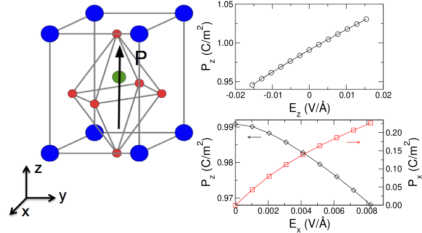
Figure 1: (Left) Sketch of a PbTiO₃ unit cell. Pb, Ti, and O atoms are represented by blue, green, and red spheres, respectively. (Right) Polarization as a function of a parallel/antiparallel electric field, $E_{z}$ and of a perpendicular field, $E_{x}$; in the latter case we display both $P_{x}$ and $P_{z}$, whose increase/decrease allows appreciating the rotation of ${\mathbf{P}}$.

We consider PbTiO₃ (PTO), a ferroelectric (FE) perovskite that below a Curie temperature $T_{\rm C}\approx 760$ K has a spontaneous electric polarization ${\mathbf{P}}$ associated to the off-centering of the cations with respect to the surrounding oxygen atoms Lines (1969); Rabe et al. (2007). PTO’s FE phase is tetragonal, with ${\mathbf{P}}=P_{z}(0,0,1)$ lying along one of the (pseudo)cubic directions of the perovskite lattice, as sketched in Figure 1. By applying electric fields above the so-called coercive field $E_{\rm coe}$ (which typically lies in the 10⁶–10⁷ V/cm range), it is possible to reverse such a polar distortion, even in small (nanometric) regions, so that FE domains can be written. Interestingly, recent works show that juxtaposed domains with different orientations of ${\mathbf{P}}$ can be used as phonon switches Seijas-Bellido et al. (2017) and phonon polarizers Royo et al. (2017). Here we consider $E<E_{\rm coe}$, exploiting the fact that, like most FE materials, PTO displays a rather large structural (dielectric) response to even moderate applied fields.

All our simulations of PTO are carried out within second-principles density-functional theory (SPDFT) as implemented in the SCALE-UP code Wojdeł et al. (2013); García-Fernández et al. (2016). SPDFT has a demonstrated predictive power for the key structural, vibrational and response properties of FE perovskite oxides Zubko et al. (2007); Wojdeł and Íñiguez (2014, 2014); Zubko et al. (2016); Shafer et al. (2018). Further, as most first-principles approaches, SPDFT reproduces accurately the vibrational and response properties of PTO Wojdeł et al. (2013), which are closely related to the quantities discussed here; hence, we expect our results to be quantitatively accurate. For more details on the used SPDFT methods and the technicalities of our calculations, please see the Supplemental Material (SM) sup . We also observe that, although our simulations are based on a model constructed to reproduce the behavior of bulk PbTiO₃, previous studies showed that the same model works well in a variety of conditions that differ from those considered to compute its parameters. This has been amply demonstrated, thanks e.g. to the application of the same PbTiO₃ model employed in this study, in a variety of investigations of PbTiO₃/SrTiO₃ superlattices Zubko et al. (2016); Damodaran et al. (2015); Shafer et al. (2018), which include successful comparisons with first-principles calculations and literature Aguado-Puente and Junquera (2012) as well as with experiment. Hence, the employed models are transferable to treat the most common thin film and superlattice geometries.

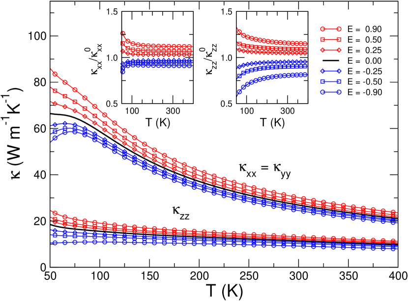
Figure 2: Thermal conductivity as a function of temperature for different values of the parallel ($E_{z}>0$) and antiparallel ($E_{z}<0$) electric field. The inset shows the relative change of the thermal conductivity as the ratio of its value with and without external field, $\kappa_{xx}/\kappa_{xx}^{0}$ (left) and $\kappa_{zz}/\kappa_{zz}^{0}$ (right). Fields are given in unit of the parallel coercive field, $E_{{\rm coe},z}$

For the calculation of the thermal conductivity tensor, we proceed as follows. For each applied field, we first relax the structure by means of a Monte Carlo simulated annealing, automatically accounting for all dielectric and piezoelectric effects that may impact the thermal conductivity Sahoo (2012). Then, we calculate the second-order interatomic force constants (IFCs) by finite differences in a $8\times 8\times 8$ supercell Togo and Tanaka (2015). We use the same supercell to compute third-order IFCs Li et al. (2014), considering interactions up fourth (twelfth) nearest-neighbors for parallel (perpendicular) fields, which we check provides good convergence. We then use the IFCs to calculate the anharmonic scattering rates and solve numerically the linearized Boltzmann Transport Equation (BTE), employing the iterative method implemented in the ShengBTE code Li et al. (2014) on a $8\times 8\times 8$ ${\bf q}$-point grid. Scattering from isotopic disorder is accounted for within the model of Tamura Tamura (1983).

The lattice thermal conductivity is then obtained as

$$\kappa_{ij}=\sum_{\lambda}\kappa_{ij,\lambda}=C\sum_{\lambda}f_{\lambda}(f_{\lambda}+1)(h\nu_{\lambda})^{2}v_{i,\lambda}F_{j,\lambda},$$ (1)

where $i$ and $j$ are the spatial directions $x$, $y$, and $z$. $C^{-1}=k_{B}T^{2}\Omega N$, where $k_{B}$, $h$, $T$, $\Omega$ and $N$ are, respectively, Boltzmann’s constant, Planck’s constant, the temperature, the volume of the 5-atom unit cell, and the number of ${\bf q}$-points. The sum runs over all phonon modes, the index $\lambda$ including both ${\bf q}$-point and phonon band. $f_{\lambda}$ is the equilibrium Bose-Einstein distribution function, and $\nu_{\lambda}$ and $v_{i,\lambda}$ are, respectively, the frequency and group velocity of phonon $\lambda$. The mean free displacement $F_{j,\lambda}$ is initially taken to be equal to $\tau_{\lambda}v_{j,\lambda}$, where $\tau_{\lambda}$ is the lifetime of mode $\lambda$ within the relaxation time approximation (RTA). Starting from this guess, the solution is then obtained iteratively and $F_{j,\lambda}$ takes the general form $\tau_{\lambda}(v_{j,\lambda}+\Delta_{j,\lambda})$, where the correction $\Delta_{\lambda}$ captures the changes in the heat current associated to the deviations in the phonon populations computed at the RTA level Li et al. (2012b); Torres et al. (2017).

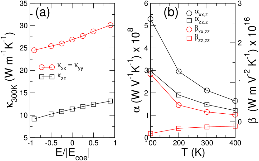
Figure 3: (a) Dependence on the electric field, $E_{z}$, of the room temperature thermal conductivity. (b) Coefficients ${\bf\alpha}$ and ${\bf\beta}$ of Eq. 2 as a function of temperature for fields applied parallel to the ${\mathbf{P}}$ vector.

Our calculations thus yield $\kappa_{ij}$ as a function of applied field and temperature, and we fit our results to

$$\kappa_{ij}(T,{\mathbf{E}})=\kappa_{ij}^{0}(T)+\sum_{k}\alpha_{ij,k}(T)E_{k}+\sum_{kl}\beta_{ij,kl}(T)E_{k}E_{l}\;,$$ (2)

where we introduce the thermal-response tensors $\bm{\alpha}$ and $\bm{\beta}$, $\bm{\kappa}^{0}$ being the conductivity at zero field. Note that, because of the high tetragonal symmetry of PTO’s FE phase ($P4mm$ space group), the number of independent tensor components in Eq. (2) is small. For example, we have $\kappa^{0}_{ij}=\delta_{ij}\kappa^{0}_{ii}$, and $\kappa^{0}_{xx}=\kappa^{0}_{yy}\neq\kappa^{0}_{zz}$. Here we focus on the behavior of $\kappa_{xx}$, $\kappa_{yy}$, and $\kappa_{zz}$ as a function of fields parallel (along $z$) and perpendicular (along $x$) to $P_{z}$. We thus calculate $\alpha_{xx,z}=\alpha_{yy,z}$ and $\alpha_{zz,z}$, noting that $\alpha_{ii,x}=\alpha_{ii,y}=0$ by symmetry; and we also calculate $\beta_{xx,xx}$, $\beta_{yy,xx}$, and $\beta_{zz,xx}$, as well as $\beta_{xx,zz}=\beta_{yy,zz}$ and $\beta_{zz,zz}$.

To explore the linear and non-linear responses, we consider field values in a range up to 90% of the theoretical $E_{\rm coe}$. Working with an idealized monodomain PTO state with $P_{z}>0$, our predicted coercive fields are $E_{{\rm coe},z}\approx-1.5\cdot 10^{8}$ V/m (to reverse $P_{z}$ to $-P_{z}$) and $E_{{\rm coe},x}\approx 8.2\cdot 10^{7}$ V/m (to rotate from $P_{z}$ to $P_{x}$, a symmetry-equivalent $x$-polarized FE phase). These fields are relatively large when compared with experimental values, an issue that is typical of first-principles works on FE switching Xu et al. (2017) and which is probably related, e.g., to the absence of nucleation centers for the polarization reversal (defects, interfaces) in the simulations. This matter is not important here. Incidentally, note that it is customary to apply fields as large as these ones to FE thin films, using voltages of a few hundreds meV.

Let us discuss first the response to fields ${\mathbf{E}}=E_{z}(0,0,1)$, which can be parallel ($E_{z}>0$) or antiparallel ($E_{z}<0$) to the electric polarization $P_{z}>0$ (see the SM for the hysteretic response). Figure 2 shows the thermal conductivity components $\kappa_{xx}$ and $\kappa_{zz}$, as a function of temperature, for several values of $E_{z}$. Let us first note that the zero-field conductivities feature a considerable anisotropy, with, e.g., $\kappa_{xx}^{0}=26.9$ W m^-1K^-1 and $\kappa_{zz}^{0}=11.4$ W m^-1K^-1 at room temperature ($T_{\rm room}$). This is a direct consequence of the FE distortion along $z$, and suggests that, if the electric field is able to affect the polarization considerably, it will also have a significant effect in the conductivity. This is indeed what we find. As shown in Figure 2, parallel fields yield an increase of both $\kappa_{xx}$ and $\kappa_{zz}$, while antiparallel fields cause a decrease. To better appreciate this effect we plot the relative variation of the thermal conductivities, $\kappa_{xx}/\kappa_{xx}^{0}$ and $\kappa_{zz}/\kappa_{zz}^{0}$ in the inset.

Further insight can be gathered from Figure 3a, which shows the variation of both $\bm{\kappa}$ components as a function of $E_{z}$ at $T_{\rm room}$. The obtained smooth behavior can be easily fitted using the quadratic expression in Eq. (2), and Figure 3b shows the $T$-dependence of the corresponding $\bm{\alpha}$ and $\bm{\beta}$ coefficients. The linear response clearly dominates, with room-temperature values of $\alpha_{zz,z}=1.47\cdot 10^{-8}$W V^-1K^-1 and $\alpha_{xx,z}=2.11\cdot 10^{-8}$ W V^-1K^-1. As regards the magnitude of the effect, for $E_{z}=0.5\times E_{{\rm coe},z}$ at $T_{\rm room}$ we obtain changes of about 7% and 9% in $\kappa_{xx}$ and $\kappa_{zz}$, respectively. These large effects are ultimately a consequence of PTO’s considerable structural response to the applied fields, as evidenced by the variation of $P_{z}$ shown in Figure 1. The corresponding lattice contribution to the dielectric susceptibility is about 31.

To gain further insight into these results, we find it convenient to analyze Eq. (1) in the following way. First, we group all the terms that are explicitly dependent on the phonon frequencies by introducing $\theta_{\lambda}=f_{\lambda}(f_{\lambda}+1)(h\nu_{\lambda})^{2}$, and write the field-induced change of $\kappa_{ij}$ as

$$\begin{split}\Delta\kappa_{ij}=&\;\;\kappa_{ij}-\kappa^{0}_{ij}=\sum_{\lambda}\Delta\kappa_{ij,\lambda}\\ =&\;\;C\sum_{\lambda}[\Delta\theta_{\lambda}v^{0}_{i,\lambda}F^{0}_{j,\lambda}+\theta^{0}_{\lambda}\Delta v_{i,\lambda}F^{0}_{j,\lambda}\\ &\;\;+\theta^{0}_{\lambda}v^{0}_{i,\lambda}\Delta F_{j,\lambda}+{\cal R}_{ij,\lambda}]\;,\end{split}$$ (3)

where the superscript “0” indicates zero-field quantities, with $\Delta g=g-g^{0}$ for any magnitude $g$. This expression allows us to readily identify changes that are dominated by only one of the factors ($\theta_{\lambda}$, $v_{i,\lambda}$, $F_{j,\lambda}$) entering the mode conductivity, while ${\cal R}_{ij,\lambda}$ captures any lingering changes. (In the limit of small applied fields ${\cal R}_{ij,\lambda}\rightarrow 0$.) Further, we can group the changes in the mode conductivities in energy intervals, using the zero-field frequencies to assign specific modes to specific intervals, and thus plot Figure 4 to analyze the $E_{z}$-induced changes in $\kappa_{xx}$ and $\kappa_{zz}$.

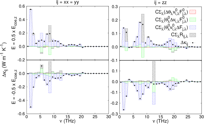
Figure 4: The different terms of Eq. 3 in the case of a parallel field, $E_{z}=0.5\times E_{{\rm coe},z}$ (upper row) and of an antiparallel field, $E_{z}=-0.5\times E_{{\rm coe},z}$ (bottom row). The dots indicate the variation of the total contribution to the thermal conductivity in a given frequency interval, i.e. $\Delta\kappa_{ij}$ in Eq. 3.

Two important observations can be drawn from this figure. On the one hand, the change of $\kappa_{xx}$ and $\kappa_{yy}$ does not depend on a particular group of phonons. Rather, the complete spectrum contributes to it, in a way that is rather homogeneous. Thus, for example, we have $\Delta\kappa_{zz}>0$ for $E_{z}>0$, where the total positive change is the result of a majority of phonons having positive $\Delta\kappa_{zz,\lambda}>0$ contributions. (Also, note the approximate symmetry of the results for $+E_{z}$ and $-E_{z}$, which is consistent with the dominant linear effect.) On the other hand, for most of the phonon spectrum, it is the change in mean free displacements that dominates the variation of the conductivity.

We can better understand the changes in $F_{j,\lambda}$ as follows. First, we can simplify our discussion by noting that $F_{j,\lambda}=\tau_{\lambda}(v_{j,\lambda}+\Delta_{j,\lambda})\approx\tau_{\lambda}v_{j,\lambda}$, as we observe that the correction to the RTA is small, typically below a 10%. Then, we find that the changes in phonon lifetimes dominate over the variations of the group velocities, which is consistent with the relatively modest impact of the $\Delta v_{j,\lambda}$ term shown in Figure 4. Further, as described in the SM and Ref. Li et al., 2014, we have $\tau_{\lambda}^{-1}\sim f_{\lambda^{\prime}}\times(\nu_{\lambda}\nu_{\lambda^{\prime}}\nu_{\lambda^{\prime\prime}})^{-1}$, where $\lambda^{\prime}$ and $\lambda^{\prime\prime}$ label modes that interact with $\lambda$ via a three-phonon scattering process. Hence, for example, if most phonons were to harden under application of a field $E_{z}>0$, the phonon frequencies $\{\nu_{\lambda}\}$ would generally increase and the populations $\{f_{\lambda}\}$ decrease, which would yield an increase of the lifetimes $\{\tau_{\lambda}\}$. This is precisely what we have in our calculations, as the average phonon frequency changes from $\bar{\nu}^{0}=9.96$ THz to $\bar{\nu}=10.05$ THz for $E_{z}=0.5\times E_{{\rm coe},z}$, resulting in generally longer lifetimes and larger thermal conductivity. In contrast, for $E_{z}=-0.5\times E_{{\rm coe},z}$ we obtain $\bar{\nu}=9.87$ THz, with generally shorter lifetimes and greater thermal resistance fre . Indeed, we find that this is the dominant effect explaining our results for $\kappa_{xx}$ and $\kappa_{zz}$ under fields that are (anti)parallel to the polarization $P_{z}$.

The fact that most of PTO’s phonon bands become harder for $E_{z}>0$ (softer for $E_{z}<0$) may seem surprising at first; yet, we believe it can be rationalized as follows. According to our simulations, the application of a parallel field has two main effects. On one hand, the cell volume grows moderately. For example, we get $\Omega/\Omega^{0}=1.0018$ for $E_{z}=0.5\times E_{{\rm coe},z}$, which is a consequence of a dominant piezoelectric effect. The increased volume alone should result in a general softening (reduction) of the phonon frequencies, which is the usual behavior corresponding to a positive Grüneinsen parameter. On the other hand, $P_{z}$ grows for $E_{z}>0$, and the stronger polar distortion can also be expected to have an impact on the phonon frequencies. More precisely, in the field of phase transitions in perovskites, it is generally observed that different distortions of the cubic perovskite structure tend to compete with each other, implying that the condensation of one (e.g., the polar distortion) tends to harden the others, thus increasing the associated phonon frequencies. (See Ref. Wojdeł et al., 2013; Mercy et al., 2017) Our results suggest that this effect is dominant in PTO.

Since we attribute the changes in conductivity under $E_{z}$-field to a general hardening/softening of the phonon spectrum, it may seem strange to note in Figure 4 that the changes associated to the $\Delta\theta_{\lambda}$ term [Eq. (3)] are negligible (in fact, they are barely visible in the figure). Yet, note that, in this term, the variations of frequencies and populations tend to cancel each other, yielding a relatively small net effect.

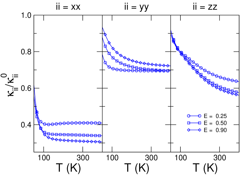
Figure 5: Ratio of the thermal conductivity with and without a perpendicular external field, $\kappa_{xx}/\kappa_{xx}^{0}$ (left), $\kappa_{yy}/\kappa_{yy}^{0}$ (center), and $\kappa_{zz}/\kappa_{zz}^{0}$ (right), as a function of temperature.

Let us now move to the case in which we apply a field ${\mathbf{E}}=E_{x}(1,0,0)$, perpendicular to the polarization, $P_{z}$. We consider $E_{x}>0$, noting that this situation is equivalent by symmetry to the application of $E_{x}<0$ or fields along $y$. Figure 5 summarizes our results, which feature a very large decrease of all the tensor components. Thus, for example, for $E_{x}=0.25\times E_{{\rm coe},x}$ at $T_{\rm room}$, we get $\kappa_{xx}/\kappa_{xx}^{0}=0.41$, $\kappa_{yy}/\kappa_{yy}^{0}=0.70$, and $\kappa_{zz}/\kappa_{zz}^{0}=0.66$. This dramatic enhancement of the thermal resistance translates into very large values of the quadratic response ${\mathbf{\beta}}$, as we obtain $\beta_{xx,xx}=-1.39\cdot 10^{-12}$ WmV^-2K^-1, $\beta_{yy,xx}=-2.26\cdot 10^{-13}$ WmV^-2K^-1, and $\beta_{zz,xx}=-6.51\cdot 10^{-14}$ WmV^-2K^-1 at $T_{\rm room}$.

Figure 6 shows the analysis based on Eq. (3), applied to the change in $\kappa_{xx}$ at $T_{\rm room}$ for a field $E_{x}=0.5\times E_{{\rm coe},x}$, which is a representative case. As above, we find that the total $\Delta\kappa_{xx}$ is the result of contributions spanning the whole phonon spectrum, and dominated by the changes in mean free paths. Also as above, we find that it is the change in the phonon lifetimes what controls $\Delta F_{j,\lambda}$; yet, at variance with the case of the $E_{z}$-fields, the present effect cannot be attributed to a general shift of frequencies. Indeed, we find that the $E_{x}$-field tends to harden the phonon spectrum (e.g., we obtain $\bar{\nu}=10.02$ THz for $E_{x}=0.5\times E_{{\rm coe},x}$). According to our above argument to explain the response to $E_{z}$-fields, the larger frequencies should result in longer lifetimes and an increased conductivity; yet, the effect of the perpendicular fields is just the opposite, with increased resistivity. Interestingly, a further analysis of our results reveals that, in this case, the field-dependence of the lifetimes is dominated by the three-phonon scattering matrix $V_{\lambda\lambda^{\prime}\lambda^{\prime\prime}}$, which controls the phonon decay as $\tau_{\lambda}^{-1}\sim|V_{\lambda\lambda^{\prime}\lambda^{\prime\prime}}|^{2}$ Li et al. (2014). More specifically, we find that the $E_{x}$-field activates a large number of new scattering processes due to the symmetry breaking that it causes. (An $E_{z}$-field does not change the symmetry of PTO’s $P_{z}$-polarized phase, and the proliferation of scattering events does not occur in that case.) This effect affects the whole phonon spectrum, and its magnitude naturally scales with the structural symmetry breaking caused by $E_{x}$, which is rather considerable given the large dielectric response of PTO to such a perturbation (for the corresponding susceptibility we obtain $\chi_{xx}\approx 304$; see Figure 1). Such a strong response to a transversal field is related to the “easy polarization rotation” that is well-known in FE perovskite oxides Fu and Cohen (2000); Bellaiche et al. (2000).

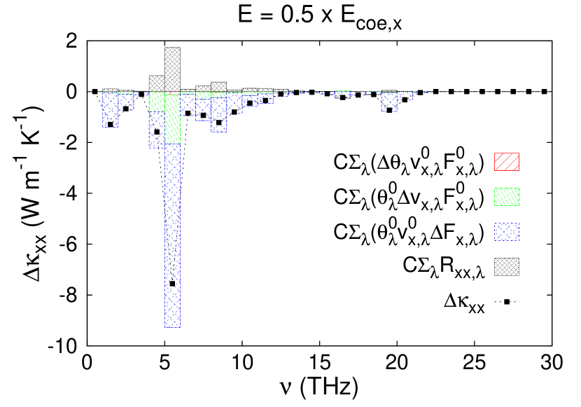
Figure 6: The different terms of Eq. 3 in the case of a perpendicular field, $E_{x}=0.5\times E_{{\rm coe},x}$ The dots indicate the variation of the total contribution to the thermal conductivity in a given frequency interval, i.e. $\Delta\kappa_{xx}$ in Eq. 3.

Interestingly, we also observe a field-induced coupling of the $x$ and $z$ directions – i.e., those along which the initial ${\mathbf{P}}$ and the applied $E_{x}$-field are oriented – in the thermal conductivity tensor. We obtain values of $\kappa_{xz}$ and $\kappa_{zx}$ that are not negligible, of the same order of those in porous Gesele et al. (1997); Dettori et al. (2015) or amorphous materials Zink et al. (2006). Their temperature dependence for applied fields is shown in the SM. This non-zero components imply that, e.g., a thermal gradient along $x$ results in a heat flux, not only along $x$, but also along $z$.

In conclusion, we have reported evidence of the coupling between electric field and thermal conductivity in a ferroelectric perovskite. We have shown that an electric field perpendicular to the spontaneous polarization greatly increases the thermal resistivity, the underlying physical mechanism being the breaking of the symmetry of the lattice, which activates new scattering processes with a concomitant reduction of the lifetimes of phonons throughout the vibrational spectrum. On the other hand, for parallel fields that do not activate new scattering processes, we observe a linear variation of the thermal conductivity, which can grow or decrease depending on the sign of the applied field. This linear effect is controlled by the overall hardening/softening of the phonon modes. The predicted behaviors open the way to a fully-electric control of phonon transport. As the underlying physical principle is the manipulation of polar modes, these results can potentially be extended to a broader class of materials, possibly with even larger responses. Finally, we note that the symmetry breaking that leads to the largest changes in the thermal conductivity can also be achieved in other ways, such as mechanical strains, that do not involve electric fields. Implementations of these concepts in a realistic device will have to take into account that substrates and additional layers will provide alternative heat transport channels and that the thermal contact resistance Yazji et al. (2015, 2016) may complicate our taking advantage of the controllable transport properties of the ferroelectric layer. These issues, however, admittedly fall beyond the scope of the present manuscript.