Triple Point of a Scalar Field Theory on a Fuzzy Sphere

Abstract

The model of a scalar field with quartic self-interaction on the fuzzy sphere has three known phases: a uniformly ordered phase, a disordered phase and a non-uniformly ordered phase, the last of which has no classical counterpart. These three phases are expected to meet at a triple point. By studying the infinite matrix size limit, we locate the position of this triple point to within a small triangle in terms of the parameters of the model. We find the triple point is closer to the coordinate origin of the phase diagram than previous estimates but broadly consistent with recent analytic predictions.

Keywords : Field theory, fuzzy sphere, triple point.

1 Introduction

Noncommutative coordinates appear in various areas of physics. Sometimes they emerge as an effective description of a physical system hall ; Fujii:2005kg or as a fundamental structure of the underlying space Grosse:1996mz ; Ydri:2001pv ; Grosse:1998gn ; DiFrancesco:1993cyw . Most notably, many of the candidate theories for quantum gravity predict such structure when approaching the Planck scale Doplicher:1994tu ; Seiberg:1999vs ; Witten:1986 .

Though noncommutativity was initially thought to provide a regularisation of field theories, it was quickly realised that this is not the case. In its fuzzy incarnation Madore:1991bw , where the number of degrees of freedom is finite, it can still be an effective regularisation scheme; especially in bosonic theories, where the underlying symmetries, for example, the rotational symmetry in the case of the fuzzy sphere, are preserved. Such theories are nonlocal and typically suffer from the infamous UV/IR mixing problem Chu:2001xi . As a result, phase diagrams of these theories differ from their commutative counterparts (even after taking what one would expect to be the commutative limit).

Noncommutative (or fuzzy) spaces and field theories on them have been studied extensively both analytically Dolan:2001gn ; Chu:2001xi ; Tekel:2017nzf ; Polychronakos:2013nca ; Tekel:2016jbp ; Tekel:2015zga ; Tekel:2015uza ; Grosse:1995jt ; Iso:2001mg ; OConnor:2007pvc ; OConnor:2007ibg ; Rea:2015wta ; CarowWatamura:1998jn ; Madore:1991bw and numerically GarciaFlores:2009hf ; Ydri:2014rea ; Ydri:2015vba ; Panero:2006bx ; Ydri:2015zba ; Vachovski ; Sabella-Garnier:2017svs . A good example is the scalar field theory with a quartic potential on a fuzzy sphere, i.e. the fuzzy $\Phi^{4}$ model. The phase diagram is controlled by the triple point, from which the phase boundaries radiate outwards and divide the plane into three distinct phase regions. The goal of this paper is to locate the triple point of the fuzzy $\Phi^{4}$ model as precisely as possible.

Earlier studies GarciaFlores:2009hf ; Ydri:2014rea used rather small matrix sizes and linear extrapolation from relatively far from the triple point to infer its location. We provide a reasonably precise estimate of its position in the $N\rightarrow\infty$ limit and find good evidence that the three known phases of the model do in fact meet at a well defined triple point. We find it to be located much closer to the origin than previous studies estimated, but in reasonably good agreement with results using an analytic approximation initiated in OConnor:2007ibg and recently further developed in Tekel:2017nzf ; for other studies in this direction see also Polychronakos:2013nca ; Rea:2015wta .

The paper is structured as follows. Section 2 describes the $\Phi^{4}$ model on a fuzzy sphere. Section 3 describes our approach and basic results. The final section is devoted to our conclusions.

2 The fuzzy $\phi^{4}$ model

A real scalar field theory with $\phi^{4}$ potential on a (commutative) sphere of radius $R$ is described by the action

$$S[\phi]=\int\limits_{\textbf{S}^{2}}d\Omega\left[\frac{1}{2}\phi\Delta\phi+\frac{rR^{2}}{2}\phi^{2}+\frac{gR^{2}}{4!}\phi^{4}\right],$$ (1)

where $\Delta=-\nabla^{2}$ is the Laplacian (with positive spectrum) on the sphere, $r$ is the mass parameter (which can be negative), $g$ is the coupling constant and $d\Omega$ is the volume form on the unit two-sphere. When $r>0$ the potential is minimised by a configuration with $\langle\phi\rangle=0$. For sufficiently small (and negative) $r$, the potential has two minima $\langle\phi\rangle=\pm\phi_{0}$; in the infinite volume limit the system spontaneously breaks the ${\mathbb{Z}}_{2}$ symmetry and oscillates around one of them. When statistical fluctuations are taken into account the model is in the universality class of the two dimensional Ising model and the transition line is described by a conformal field theory. Lattice simulations of the two-dimensional commutative model ($\phi^{4}_{2}$) on the plane were performed in Loinaz:1997az ; Bosetti:2015lsa , where the transition line in the $(r,g)$ plane was measured. A recent study of the two-dimensional commutative model was performed using a finite element approximation to the two-sphere in Brower:2016moq and they find good agreement with results expected from conformal field theory and renormalisation group studies.

We are interested in the non-commutative version of this scalar field defined on a fuzzy sphere specified by the action

$$S_{N}[\Phi]=\mbox{Tr }\left[a\ \Phi^{\dagger}\mathcal{L}^{2}\Phi+b\ \Phi^{2}+c\ \Phi^{4}\right],$$ (2)

where $\Phi$ is a Hermitian $N\times N$ matrix, $\mathcal{L}^{2}\Phi=[L_{i},[L_{i},\Phi]]$ with $L_{i},i=1,2,3$ being the usual $SU(2)$ generators in the irreducible representation of dimension $N$. This action can be seen as a regularisation of the commutative model by defining the matrix $\Phi$ associated with a field configuration $\phi$ as

$$\Phi=\int\limits_{\textbf{S}^{2}}d\Omega\ \rho(\hat{n})\phi(\hat{n}),\quad\hbox{where}\quad\rho(\hat{n})=\sum_{l,m=0}^{N-1}\hat{Y}_{lm}Y^{\dagger}_{lm}(\hat{n}),$$ (3)

$Y_{lm}(\hat{n})$ are the standard spherical harmonics and $\hat{Y}_{lm}$ are the polatisation tensors; details of the map $\rho(\hat{n})$ can be found in Dolan:2006tx . Its effect can be understood by expanding the field $\phi$ in spherical harmonics. The map (3) replaces spherical harmonics with polarisation tensors up to the maximum angular momentum allowed by the matrix size, i.e. $L=N-1$, higher modes being cut off. With this identification one can establish that

$$\lim_{N\rightarrow\infty}\left|S[\phi]-S_{N}[\Phi]\right|\rightarrow 0$$ (4)

provided we identify $a=\frac{2\pi}{N},b=\frac{2\pi rR^{2}}{N}$ and $c=\frac{\pi gR^{2}}{6N}$.

From the above construction, we see that a field on a fuzzy sphere (or any other similarly constructed fuzzy space) has only a finite number of degrees of freedom, but contrary to a lattice discretisation, the underlying rotational symmetry is preserved.

We are interested in the statistical mechanics of this model where the mean value of an observable is defined as

$$\langle\mathcal{O}(\Phi)\rangle=\frac{\int d[\Phi]\mathcal{O}(\Phi)e^{-S_{N}[\Phi]}}{\int d[\Phi]e^{-S_{N}[\Phi]}},$$ (5)

and we integrate over all possible (Hermitian) matrix configurations. Without loss of generality, we can rescale the matrix $\Phi$ to make $a=1$ and use the scale-free parameters $\tilde{b}=b/(aN^{\frac{3}{2}}),\ \tilde{c}=c/(a^{2}N^{2})$ as in GarciaFlores:2009hf .

The finiteness of the number of degrees of freedom is not the only novel feature of the matrix model compared to its commutative counterpart. If there was no gradient term in (2), the action could be expressed in terms of the eigenvalues, $\lambda_{i}$, of $\Phi$. The integration would become $\int d[\Phi]\rightarrow\int\Delta^{2}(\lambda)d[\lambda]d[\theta]$, where $\Delta(\lambda)$ is the Vandermonde determinant.

As long as the observable in question depends only on $\lambda_{i}$, the integral $\int d[\theta$] gives the volume of the corresponding flag manifold and cancels in (5). The Vandermonde determinant lifted to the exponential acts as an additional logarithmic repulsion between the eigenvalues. In the large $N$ limit the pure potential model has a third order phase transition, at $b_{c}=-2\sqrt{Nc}$, to a phase where the eigenvalues are distributed between both minima of the potential and do not jump the barrier. This new phase is closely related to the additional phase present in the model (2).

The overall form of the phase diagram for the $\Phi^{4}$ model on a fuzzy sphere is the following: when $\tilde{c}$ is sufficiently large (and fixed), there are two critical values for $\tilde{b}$. For $\tilde{b}>\tilde{b}_{c_{1}}$, the system oscillates around the trivial vacuum, $\langle\lambda_{i}\rangle=0$. The eigenvalue distribution in this phase is a distorted Wigner semicircle – this is called the disordered phase. On the other hand, when $\tilde{b}<\tilde{b}_{c_{2}}$, all of the eigenvalues oscillate around the minimum of one of the pair of (deep) potential wells related by ${\mathbb{Z}}_{2}$ symmetry, $\langle\lambda_{i}\rangle=\pm\lambda_{0}$. Due to the repulsion between the eigenvalues discussed above, when $\tilde{b}_{c_{2}}<\tilde{b}<\tilde{b}_{c_{1}}$ and $\tilde{c}$ is sufficiently large, there is an additional matrix phase, which lies between the disordered and the uniform phase. It has no classical counterpart in the commutative model and is characterised by some eigenvalues in one well and rest of them in the other, $\langle\lambda_{i}\rangle={\pm}_{i}\lambda_{0}$. This phase is referred to as non-uniformly ordered.

As the coupling $\tilde{c}$ is lowered, the two transitions at $\tilde{b}_{c_{1}}$ and $\tilde{b}_{c_{2}}$ approach and eventually meet at the triple point $(\tilde{c}_{T},\tilde{b}_{T})$. For $\tilde{c}<\tilde{c}_{T}$, the non-uniformly ordered phase is absent. It is the location of this triple point we seek.

3 Methods and results

We performed hybrid Monte Carlo (HMC) Duane:1987de simulations of the model with the probability weight defined by the action (2). In contrast to the ordinary Monte Carlo method, the hybrid one includes molecular dynamics that shortens the auto-correlation length and the required computational time.

The idea of the HMC method (see e.g. HMC ) is that instead of just updating the configuration with a random impulse, one first introduces fictional momentum degrees of freedom and treats the original action as the potential for these momenta in a new Hamiltonian. The integral over the new momenta is trivial as they are Gaussian degrees of freedom. One then finds a proposed update for $\Phi$ as a solution to the discretised Hamilton equations, where the leapfrog interval and number of steps are new parameters of the simulation. One then imposes the Metropolis check on the proposed configuration. The resulting configurations are then much more decorrelated and the system thermalises more rapidly.

In a comparison of the Metropolis and HMC methods we ran test simulations generating $10^{5}$ configurations with $N=15$, $\tilde{b}=-0.1$, $\tilde{c}=0.5$. To facilitate a comparison the Metropolis algorithm was implemented with a complete matrix updated by proposing a new configuration $\Phi^{\prime}=\Phi+\epsilon_{\mbox{\tiny{M}}}P$ with $P$ choosen from a Gaussian distribution. We tuned the $\epsilon_{\mbox{\tiny{M}}}$ and the HMC step-length $\epsilon_{\mbox{\tiny{HMC}}}$ to achieve the same acceptance rate ($90\%$ for this example only) for the Metropolis and the HMC algorithms. While the former required considerably shorter step-lenght, $\epsilon_{\mbox{\tiny{M}}}\simeq\frac{\epsilon_{\mbox{\tiny{HMC}}}}{60}$, it also produced data with considerably longer auto-correlation length, $\lambda_{\mbox{\tiny{M}}}\simeq 14\lambda_{\mbox{\tiny{HMC}}}$.

In actual simulations we tried to keep the acceptance rate between 60% – 90% which differs slightly from the recommended value (we wanted to use the same value for large portions of the phase diagram to make the simulations as automated as possible) and auto-correlation lengths of the order of ten configurations or less. We typically ran $\sim 10^{3}$ values of $\tilde{b}$ and $\tilde{c}$ to construct a phase diagram with fixed $N$, each of them generating $10^{5}-10^{6}$ configurations (dropping the first $\sim 10^{4}$ steps of thermalisation).

The HMC algorithm allowed us the work with larger matrices, up to $N=127$, which we have used to extrapolate to $N\rightarrow\infty$. We have measured the value of the action for each of the Monte Carlo steps, from which the specific heat $C_{v}=\left(\langle S^{2}\rangle-\langle S\rangle^{2}\right)/N^{2}$ and the Jack-knife error estimate were obtained.

Since we are dealing with a finite size system the phase transitions are smeared and manifest themselves as (finite) peaks in the specific heat.

The strategy was to fix the value of $N$ and $\tilde{c}$ and to make simulations with multiple, slightly separated, values of $\tilde{b}$. This allowed us to plot $C_{v}(\tilde{b})$ and identify the phase transition values of $\tilde{b}$, see Figure 2. The number of data-points (simulations) for the analysed values of $N$ was of the order of thousands, which was sufficient to construct the phase diagram with the required precision.

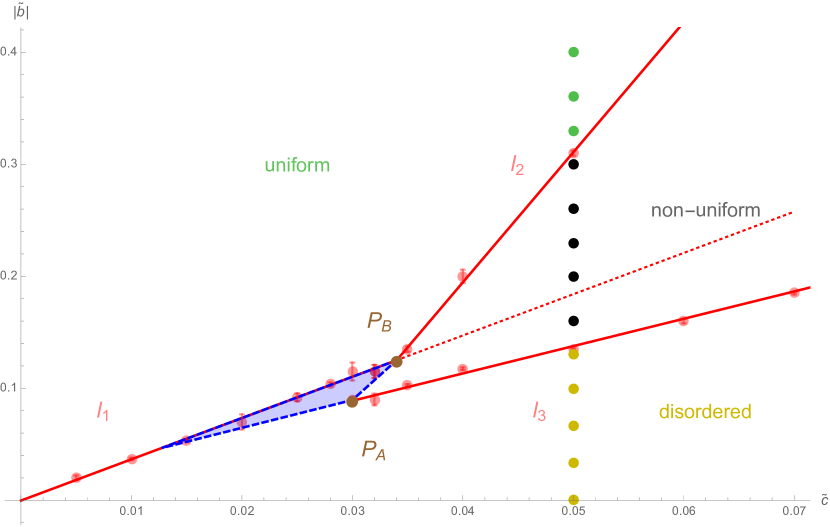
Figure 1: The phase diagram for $N=64$. Red lines are the fits of measured phase transitions, which are denoted by points with barely visible error bars. $P_{B}$ denotes the point where $l_{1}$ bends into $l_{2}$, $P_{A}$ denotes the point where $l_{3}$ emerges. The position of the triple point can be estimated to either lay in the blue triangle or, as a cruder estimate, just between these two points. The phase transitions were identified from the behaviour of the specific heat $C_{v}$, but for $\tilde{c}=0.05$ we have also checked the eigenvalue distribution directly to verify it (the colour points correspond to their respective phases). The lines are fitted as $l_{1}:|\tilde{b}|=-0.000(2)+3.68(9)\tilde{c}$, $l_{2}:|\tilde{b}|=-0.27(2)+11.6(4)\tilde{c}$, $l_{3}:|\tilde{b}|=0.015(2)+2.44(4)\tilde{c}$.

The overall structure of the phase diagram is the same for all values of $N$. There is one coexistence curve starting from the origin of the phase diagram separating the disordered and the uniformly ordered phases, denoted $l_{1}$. It bends to a new curve $l_{2}$ at a point labeled $P_{B}$. Close to $P_{B}$ a new coexistence line, $l_{3}$, appears at a point we denote $P_{A}$. The non-uniformly ordered phase exists between $l_{2}$ and $l_{3}$, the uniformly ordered phase exists above the line $l_{2}$ and the disordered one below $l_{2}$, see Figure 1. All of the coexistence curves, $l_{1},l_{2}$ and $l_{3}$, are well approximated by straight lines, at least in the vicinity of the triple point.

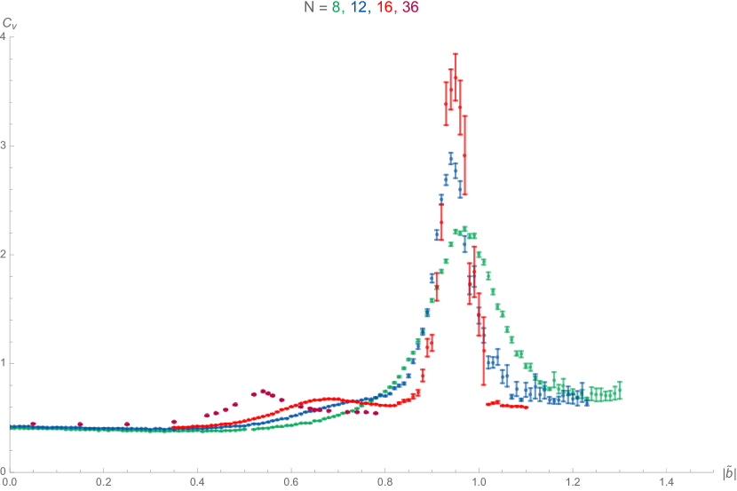
Figure 2: The specific heat for small $N$ and $\tilde{c}=0.20$. In the $N=16$ plot only the main peak corresponding to the non-uniformly to uniformly ordered phase boundary is visible. The plots for $N=12$ and $N=16$ show the emergence of the secondary peak corresponding to the disordered to non-uniformly ordered phase boundary. For $N=36$ only the latter peak is visible.

The line $l_{2}$ in Figure 1 is more correctly described as the set of values where the potential barrier separating the two phases has become too large for the fluctuations of the system to successfully jump between the phases. The specific heat in this region would be extremely large and the system can be modeled by two Gaussian distributions whose means differ but have similar standard deviations. Since the value of $\tilde{b}$ at which this occurs approaches the triple point with increasing $N$, this line provides a useful marker of the upper boundary of the triangles we use to locate the triple point. It should not be taken as the true coexistence curve. Rather the coexistence curve is a continuation of the line $l_{1}$ and we find that the two coexistence curves in the vicinity of the triple point fall on the one, surprisingly straight, line through the origin.

One can see the peaks in $C_{v}$ for different $N$ and fixed $\tilde{c}=0.20$ in Figure 2. For $N=16$ both peaks are present and one can also observe that the location of the larger peak, corresponding to the disorder-nonuniform order coexistence line, is largely insensitive to $N$ but grows rapidly with increasing $N$. Our results agree with those of the earlier studies in the region of the phase diagram accessed in those studies.

As analysed in Tekel:2017nzf , both uniform and non-uniform solutions coexist and the dominant phase is determined by the one of lower free energy. In the vicinity of the coexistence line the two states are separated by a high barrier, and the simulation can spend a large number of Monte Carlo steps oscillating around a wrong vacuum state; this makes the line $l_{2}$ hard to measure precisely–for larger $N$ it is especially difficult to maintain ergodicity in the simulations.

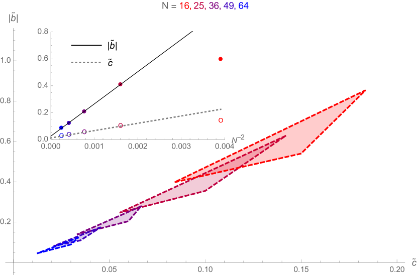
Figure 3: The progression of triangles $t_{N}$ used to estimate the position of the triple point for various values of $N$. The results for $N=16$ was not used in the extrapolation as this value of $N$ seems to be too small and this result differs from the clear trend set by the rest of the values, which are nearly perfectly fitted by a linear function of $N^{-2}$, see the small statistical errors in Table 1.

The lines $l_{1},l_{2},l_{3}$ do not intersect exactly, which is partially caused by the finiteness of $N$ and partially by the statistical errors of the measured data. Therefore, instead of meeting, they form a triangle $t_{N}=\{P_{1},P_{2},P_{3}\}$, where by definition $P_{2}\approx P_{B}$ and from our experience $P_{3}\approx P_{A}$.

It is impossible to localize the triple point exactly with a finite value of $N$, but it can be expected to be contained in the triangle $t_{N}$. We have observed that the area of $t_{N}$ declines as $N$ grows and the center of mass of its upper-half converges to a certain value – which we take to be the position of the triple point in the $N\rightarrow\infty$ limit. The systematic error of this estimate is the size (the square root of the area) of the triangle, the statistical error is that of the fitting coefficients (the coordinates of the triple point are well fitted as linear functions of $N^{-2}$).

A more straightforward and alternative approach would be to take the estimate of the triple point to be the middle-point between $P_{A}$ and $P_{B}$, the error being a half of their distance.

Another option is first to extrapolate the phase transition points for fixed $\tilde{c}$ (in the $\tilde{b}$ direction) and to construct the phase transition lines only afterward. The advantage of this method is that it allows us to measure the linear coefficients of the curves in the vicinity of the tripe point. The disadvantage is that different points converge with increasing $N$ at different rates. For example, the disordered to non-uniformly ordered transition close to the triple point requires very large matrix sizes, for our closest point even $N=127$ seemed insufficient.

Results of these three methods are gathered in Table 1. Coefficients of the curves in the $N\rightarrow\infty$ limit can be found in Figure 5.

Table 1: Estimation of the triple point.

•	$\tilde{c}$	$|\tilde{b}|$
Triangle	$0.016\pm 0.009_{\mbox{sys}}\pm 0.001_{\mbox{st}}$	$-0.031\pm 0.009_{\mbox{sys}}\pm 0.009_{\mbox{st}}$
Middle-point	$0.019\pm 0.001_{\mbox{sys}}\pm 0.002_{\mbox{st}}$	$-0.039\pm 0.015_{\mbox{sys}}\pm 0.005_{\mbox{st}}$
Extrapolation	$0.021\pm 0.002_{\mbox{sys}}$	$-0.057\pm 0.006_{\mbox{sys}}$

The previous study reported the values of $\tilde{c}=0.52,\ \tilde{b}=-2.3$ (see GarciaFlores:2009hf ) and $\tilde{c}=0.58,\ \tilde{b}=-2.49$ (see Ydri:2014rea ), but no data was gathered in the immediate vicinity of the transition due to the smallness of the matrices studied, rather the triple point was inferred from a linear extrapolation of the three coexistence curves obtained far from the triple point. The maximal matrix size used in those studies was $N=10$, which is, as we have learned, not free of small $N$ effects (when plotting the estimates of $\tilde{c},|\tilde{b}|$ versus $N^{-2}$, even the point $N=16$ deviates from the very clear trend set by $N=25,36,49,64$; see Figure 3). Also, we were able to measure the phase transition closer to the triple point, not having to rely on extrapolations from distant regions.

The new estimates for the triple point position is in reasonable accord with a recent analytic study Tekel:2017nzf which provides the values of $\tilde{c}_{T}=0.0196,\ \tilde{b}_{T}=-0.35$. This value of $\tilde{c}$ agrees very well with our estimate but the discrepancy in $\tilde{b}$ is significant and lies well outside our errors. It is probably caused by the approximations used in Tekel:2017nzf and further effort on the analytic side is expected to improve the agreement.

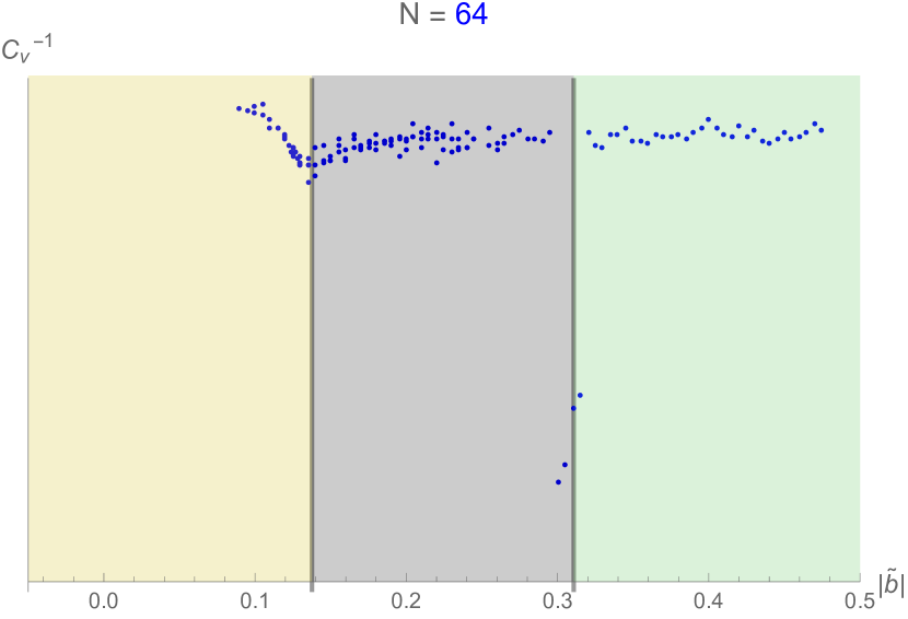
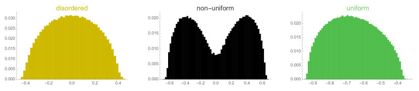
Figure 4: The top figure shows $1/C_{v}$ for $N=64$ and a range of $\tilde{b}$ that crosses both transitions. Below are shown typical eigenvalue distributions for the respective phases above, where the colour coding is matched in the two figures. The distributions were taken for $\tilde{c}=0.05$ and $-\tilde{b}=0.033333,\,0.16667$ and $0.4$ respectively using the last $4000$ configurations.

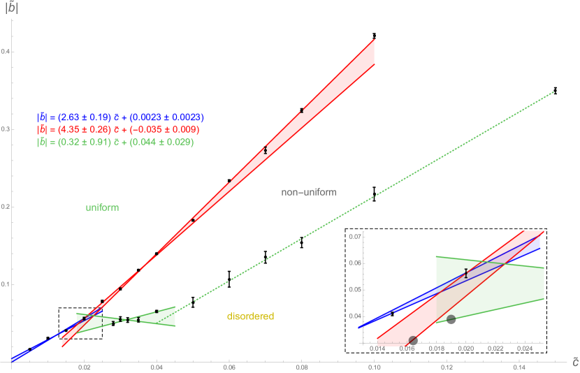
Figure 5: Phase diagram obtained by first extrapolating the phase transition points $\tilde{b}(\tilde{c})$ as $N\rightarrow\infty$ and then by fitting the lines close to the triple point. There are two or three curves for each of the transition lines because their slopes change as the triple point is approached. The coloured region is bounded by two lines – one obtained by fitting only the nearest well-resolved points, the other using also more distant ones; the correct phase transition lines should be bounded by those lines. Center of the area where these regions overlap is quoted as the third triple point estimate in Table 1. The values of used matrix sizes differ for each of the points, but were in the range $8\leq N\leq 127$. There is an interesting point where three of the boundary curves cross: $\tilde{c}=0.0226,|\tilde{b}|=0.0599$. The grey points in the zoomed plot mark the estimates obtained using the two other methods.

4 Conclusion

We have refined the position of the triple point of a scalar field theory on a fuzzy sphere by using hybrid Monte Carlo simulations and extrapolating to the $N\rightarrow\infty$ limit using matrices of size up to $N=127$.

We have used three different methods to estimate the position of the triple point, where their confidence intervals overlap we have

$$\tilde{c}_{T}=0.020\pm 0.001,\ \tilde{b}_{T}=-0.054\pm 0.003,$$ (6)

which is our best estimate for its location.

Our results are in a broad agreement with recent analytic studies of the model in Tekel:2017nzf . It is conceivable that the true triple point lies at the origin, however, our results indicate that this is not the case as the origin is many standard deviations from our estimate.

We have located the phase transitions from peaks in the specific heat $C_{v}$, but we also independently checked the eigenvalue distribution for a range of $\tilde{c}$ and various values of $\tilde{b}$ to verify the identified phases. Figure 5 shows the specific heat for $N=64$ and $\tilde{c}=0.05$ and corresponds to the column of colour points in Figure 1.

The observed behaviour of the specific heat as the triple point is approached while taking larger values of $N$, is that the main peak grows and moves to smaller values of $|\tilde{b}|$ and a new peak appears near the large one, but at smaller $|\tilde{b}|$, see Figure 2. These peaks follow the coexistence lines $l_{1}$ and $l_{3}$ of Figure 1 and are what we consider the phase boundaries of the system. While constructing the phase diagram we have observed similar behaviour further away from the triple point. More specifically, as we move away from the triple point the secondary peak gets large and yet another tertiary peak appears, which in turn grows and bifurcates. This behaviour suggests the existence of additional triple points further out along the line $l_{3}$. We conjecture that the non-uniformly ordered phase consists of a family of distinct phases separated by new coexistence lines. This issue would deserve a study on its own and we hope to return to it in the future.

We have not focused on the exact character of the phase transitions (in the large $N$ limit), but our simulations show clearly that the transition from the non-uniformly ordered to the disordered phase is first-order. This can also be seen from the rapid growth of the peaks in the specific heat in Figure 2. The transition from the disordered to the non-uniformly ordered phase appears to be third-order (as in the pure potential model) and the transition curve asymptotes to that of the matrix model for large $\tilde{c}$. The nature of the transition at small $\tilde{c}$ (the disordered to uniform order transition) is more difficult to establish and the numerical results are inconclusive. The approximate models studied in Tekel:2017nzf suggests that this transition is of second-order but unfortunately our numerical results in this region are not precise enough to support this conclusion, but also are not in conflict with it.

Our results are in accord with earlier studies GarciaFlores:2009hf and the approximate models Tekel:2017nzf whose results agree with those shown in Figure 5.

The fact that the triple point lies so close to the origin suggests that one should be able to get reasonable estimates of its location from direct perturbation theory around zero coupling. We believe that such an approach is well worth further effort.

A further direction worthy of future study is the introduction of a higher derivative terms to the gradient term, Dolan:2001gn . These will further regulate the theory and when tuned appropriately, should push the triple point towards infinity – leaving only two phases that should again be in the Ising universality class.

Acknowledgment

The authors wish to acknowledge the Irish Centre for High-End Computing (ICHEC) for the provision of computational facilities and support (Project Name dsphy009c and dsphy010c). The support from Action MP1405 QSPACE of the COST foundation is gratefully acknowledged. S. Kováčik was supported by Irish Research Council funding. D. O’Connor thanks M. Vachovski and S. Kováčik thanks to Juraj Tekel for helpful discussions.

References

- [1] J. Bellissard A. van Elst, and H. Schulz-Baldes, The noncommutative geometry of the quantum Hall effect JMP, 35 (1994)
- [2] K. Fujii, From quantum optics to non-commutative geometry: A Non-commutative version of the Hopf bundle, Veronese mapping and spin representation, [quant-ph/0502174]
- [3] H. Grosse, C. Klimcik and P. Presnajder, On finite 4-D quantum field theory in noncommutative geometry, Commun. Math. Phys. 180 (1996) 429 [hep-th/9602115]
- [4] B. Ydri, Fuzzy physics, [hep-th/0110006]
- [5] H. Grosse and P. Presnajder, A noncommutative regularization of the Schwinger model, Lett. Math. Phys. 46 (1998) 61
- [6] P. Di Francesco, P. H. Ginsparg and J. Zinn-Justin, 2-D Gravity and random matrices, Phys. Rept. 254 (1995) 1 [hep-th/9306153]
- [7] S. Doplicher, K. Fredenhagen and J. E. Roberts, The Quantum structure of space-time at the Planck scale and quantum fields, Commun. Math. Phys. 172 (1995) 187 [hep-th/0303037]
- [8] N. Seiberg and E. Witten, String theory and noncommutative geometry, JHEP 9909 (1999) 032
- [9] E. Witten, Non-commutative geometry and string field theory, Nuc. Phys. B 2 (1986) 253
- [10] J. Madore, The Fuzzy sphere, Class. Quant. Grav. 9 (1992) 69
- [11] C. S. Chu, J. Madore and H. Steinacker, Scaling limits of the fuzzy sphere at one loop, JHEP 0108 (2001) 038 [hep-th/0106205]
- [12] U. Carow-Watamura and S. Watamura, Noncommutative geometry and gauge theory on fuzzy sphere, Commun. Math. Phys. 212 (2000) 395 [hep-th/9801195]
- [13] D. O’Connor and C. Saemann, Fuzzy Scalar Field Theory as a Multitrace Matrix Model, JHEP 0708 (2007) 066 [hep-th/0706.2493]
- [14] J. Tekel, Asymmetric hermitian matrix models and fuzzy field theory, [hep-th/1711.02008]
- [15] S. Rea and C. Saemann, The Phase Diagram of Scalar Field Theory on the Fuzzy Disc, JHEP 1511 (2015) 115 [hep-th/1507.05978]
- [16] A. P. Polychronakos, Effective action and phase transitions of scalar field on the fuzzy sphere, Phys. Rev. D 88 (2013) 065010 [hep-th/1306.6645]
- [17] D. O’Connor and C. Saemann, A Multitrace matrix model from fuzzy scalar field theory, [hep-th/0709.0387]
- [18] S. Iso, Y. Kimura, K. Tanaka and K. Wakatsuki, Noncommutative gauge theory on fuzzy sphere from matrix model, Nucl. Phys. B 604 (2001) 121 [hep-th/0101102]
- [19] H. Grosse, C. Klimcik and P. Presnajder, Topologically nontrivial field configurations in noncommutative geometry, Commun. Math. Phys. 178 (1996) 507 [hep-th/9510083]
- [20] J. Tekel, Matrix model approximations of fuzzy scalar field theories and their phase diagrams, JHEP 1512 (2015) 176 [hep-th/1510.07496]
- [21] J. Tekel, Phase strucutre of fuzzy field theories and multitrace matrix models, Acta Phys. Slov. 65 (2015) 369 [hep-th/1512.00689]
- [22] J. Tekel, Phase diagram of scalar field theory on fuzzy sphere and multitrace matrix models, PoS CORFU 2015 (2016) 123 [hep-th/1601.05628]
- [23] B. P. Dolan, D. O’Connor and P. Presnajder, Matrix phi**4 models on the fuzzy sphere and their continuum limits, JHEP 0203 (2002) 013 [hep-th/0109084]
- [24] F. Garcia Flores, X. Martin and D. O’Connor, Simulation of a scalar field on a fuzzy sphere, Int. J. Mod. Phys. A 24 (2009) 3917 [hep-lat/0903.1986]
- [25] S. Duane, A. D. Kennedy, B. J. Pendleton and D. Roweth, “Hybrid Monte Carlo,” Phys. Lett. B 195 (1987) 216. doi:10.1016/0370-2693(87)91197-X
- [26] R. M. Neal, MCMC using Hamiltonian dynamics in S. Brooks, A. Gelman, G. Jones and X. Meng, Handbook of Markov Chain Monte Carlo, CRC Press, (2011)
- [27] B. Ydri, New algorithm and phase diagram of noncommutative on the fuzzy sphere, JHEP 1403 (2014) 065 [hep-th/1401.1529]
- [28] M. Panero, Numerical simulations of a non-commutative theory: The Scalar model on the fuzzy sphere, JHEP 0705 (2007) 082 [hep-th/0608202]
- [29] P. Sabella-Garnier, Time dependence of entanglement entropy on the fuzzy sphere, JHEP 1708 (2017) 121 [hep-th/1705.01969]
- [30] B. Ydri, K. Ramda and A. Rouag, Phase diagrams of the multitrace quartic matrix models of noncommutative theory, Phys. Rev. D 93 (2016) no.6, 065056 [hep-th/1509.03726]
- [31] B. Ydri, Computational Physics: An Introduction to Monte Carlo Simulations of Matrix Field Theory, [hep-lat/1506.02567]
- [32] M. P. Vachovski, Numerical studies of the critical behaviour of non-commutative field theories, Ph.D. thesis
- [33] W. Loinaz and R. S. Willey, Monte Carlo simulation calculation of critical coupling constant for continuum phi**4 in two-dimensions, Phys. Rev. D 58 (1998) 076003 [hep-lat/9712008]
- [34] P. Bosetti, B. De Palma and M. Guagnelli, Monte Carlo determination of the critical coupling in theory, Phys. Rev. D 92 (2015) no.3, 034509 [hep-lat:1506.08587]
- [35] R. C. Brower, G. Fleming, A. Gasbarro, T. Raben, C. I. Tan and E. Weinberg, Quantum Finite Elements for Lattice Field Theory, PoS LATTICE 2015 (2016) 296 [hep-lat/1601.01367]
- [36] B. P. Dolan, I. Huet, S. Murray and D. O’Connor, Noncommutative vector bundles over fuzzy CP**N and their covariant derivatives, JHEP 0707 (2007) 007 [hep-th/0611209]