PT-symmetric quantum graphs

Abstract

We consider PT-symmetrically branched quantum wires, in which the branching points provide PT-symmetric boundary conditions for the Schrödinger equation on a graph. For such PT-symmetric quantum graph we derive general boundary conditions which keep the Hamiltonian as PT-symmetric with real eigenvalues and positively defined norm. Explicit boundary conditions which are consistent with the general PT-symmetric boundary conditions are presented. Secular equations for finding the eigenvalues of the quantum graph are derived. Breaking of the Kirchhoff rule at the branching point is shown. Experimental realization of PT-symmetric quantum graphs on branched optical waveguides is discussed.

Introduction. PT-symmetric quantum systems attracted much attention since from the pioneering paper CMB1 , where the authors showed that a quantum system with non-Hermitian but PT-symmetric Hamiltonian can have a set of eigenstates with real eigenvalues (a real spectrum). Later it was strictly shown that the Hermiticity of the Hamiltonian is not a necessary condition for the realness of its eigenvalues. Quantum mechanics of such systems has become rapidly developing topic by now and called PT-symmetric quantum mechanics (see papers CMB2 -ptbox for review of recent developments on the topic). Different aspects of PT-symmetric quantum physics have been studied in huge number of papers published during past two decades. These studies allowed to construct complete theory of PT-symmetric quantum system, including PT-symmetric field theory CMB07 ; CMB11 . Experimental realization of such systems was also subject for extensive research. The latter has been done mainly in optics Makris ; Nature ; UFN ; Konotop . Some other PT-symmetric systems are discussed recently in the literature Chit ; Longhi . PT-symmetric relativistic system are also studied in PTSD1 ; PTSD2 . General condition for PT-symmetry has been derived in terms of so-called PT-symmetric inner product. However, since such condition does not provide positively defined norm of the eigenvalues, its extension in terms CPT-symmetric inner product was proposed in CMB5 ; CMB9 ; CMB11 . Similarly to the case of Hermiticity, PT-symmetry can be introduced either through the complex potential or by imposing proper boundary conditions which provides such symmetry via the inner product CMB5 ; CMB11 . Different types of complex potentials providing PT-symmetry in Hamiltonian have been considered in CMB9 ; CMB11 . Introducing PT-symmetry in terms of proper boundary conditions was studied for particle-in-box system in CMB13 ; Znojil ; Znojil2 ; ptbox . Certain progress is also done in nonlinear extension of PT-symmetric systems UFN ; Konotop ; Panos . Spectral properties of the Laplace operators on graph in the presence of PT- and reflection symmetry have been considered in Kurasov1 ; Kurasov2 .

In this Letter we consider the problem of PT-symmetric quantum graph which implies connecting quantum wires according to PT-symmetry. The latter means imposing PT-symmetric boundary conditions at the branching point of the quantum graph. Quantum graph itself is a branched system of quantum wires. Branching (connection) rule is called topology of a graph and given in terms of adjacency matrix Uzy1 ; Uzy2 . When length are assigned to the bonds of a graph, it is called a metric graph. The vertex (branching)boundary condition for Schrödinger equation on a quantum graph are imposed as providing Hermiticity of the Hamiltonian. First strict study of quantum graphs as branched quantum wires was presented in Exner1 . General boundary conditions for the Schrödinger equation on graphs were derived in terms of Hermitian inner product Kost . Later such boundary condition have been derived for Dirac equation on graphs in Bolte . Spectral statistics and manifestation of quantum chaos was studied in Uzy1 ; Uzy2 . Different aspects of the Schrödinger operator on graphs have been studied in the Refs.Kuchment04 -Exner15 . Experimental realization of quantum graphs on optical microwave networks has been discussed in Hul . Nonlinear extension of the wave dynamics in networks considered in Our1 ; Our2 ; Our3 . Here we derive PT- symmetric analogs of the Hermitian boundary conditions for quantum graphs which have been derived first in the Ref.Kost . Such conditions are needed to construct PT-symmetric quantum graphs. Also, we consider special cases of the boundary conditions which are consistent with the general ones and obtain secular equation for finding the eigenvalues of the Schrodinger operator on graphs. By solving numerically such secular equation we show that the eigenvalues of the problem are real, the norm is positively defined and the Kirchhoff rule is broken at the branching point of a graph. Motivation for the study of PT-symmetric quantum graphs mainly comes from the possibility for their experimental realization in optical waveguide networks. Such networks can be constructed by connecting optical waveguides via dissipative, optically absorbing material. Also, condensed matter realizations using branched graphene nanoribbons or branched polymers can be considered.
PT-symmetric boundary conditions. Let us first recall construction of Hermitian boundary conditions for quantum graphs which were derived in Kost . The Schrödinger equation on metric star graph with $N$ finite bonds, $b_{j}\sim(0;L_{j}),\,j=1,2,...,N$ can be written as (in units $\hbar=2m=1$)

$$-\frac{d^{2}\psi_{j}}{dx^{2}}=k^{2}\psi_{j}\,\,,\,x\in(0;L_{j}),j=1,2,3...,N,$$ (1)

where $L_{j}$ length of the $j$th bond.

The inner product of two functions, $\phi$ and $\psi$ on a graph can be written as Kost

$$\langle\phi,\psi\rangle=\sum_{j=1}^{N}\int_{0}^{L}\phi_{j}(x)\psi^{*}_{j}(x)dx.$$ (2)

Here we introduce so-called skew-Hermitian product on graph, which is defined for arbitrary differential operator, $H$ as Kost

$$\Omega(\psi,\phi)=\langle H\psi,\phi\rangle-\langle\psi,H\phi\rangle.$$ (3)

Then for Eq.(3) general Hermitian boundary conditions on metric star graph can be written as Kost

$$\Omega(\psi,\phi)=-\sum_{j}^{N}[\phi_{j}^{*}(0)\frac{d\psi_{j}(0)}{dx}-\psi_{j}(0)\frac{d\phi_{j}^{*}(0)}{dx}]$$

$$+\sum_{j}^{N}[\phi_{j}^{*}(L)\frac{d\psi_{j}(L)}{dx}-\psi_{j}(L)\frac{d\phi_{j}^{*}(L)}{dx}]=0$$ (4)

Eq.(4) is provides the boundary conditions keeping the Schrödinger operator on metric star graph as self-adjoint and can be rewritten in compact form as Kost

$${\bf A}\Psi+{\bf B}\Psi^{\prime}=0,$$ (5)

where

$$rank({\bf A})=rank({\bf B})=2N,$$

$${\bf AB^{\dagger}}={\bf BA^{\dagger}}.$$ (6)

Our purpose is to derive PT-symmetric analogs of Eqs.(3) and (4). To do this, one should use in Eq.(2) PT-symmetric inner product, instead the Hermitian inner product. Such inner product is given by CMB5 ; CMB9 ; CMB7

$$\langle\psi,\varphi\rangle_{PT}=\underset{j=1}{\overset{N}{\sum}}\underset{0}{\overset{L_{j}}{\int}}PT\psi_{j}(x)\cdot\varphi_{j}(x)dx.$$ (7)

Then using the relations

$$P\psi_{j}(x)=\psi_{j}(L_{j}-x),\,T\psi_{j}(x)=\psi_{j}^{*}(x),$$ (8)

for Eq.(1), we can write PT-symmetric form as

$$\Omega(\psi,\varphi)= \langle H\psi,\varphi\rangle-\langle\psi,H\varphi\rangle$$

$$= \underset{j=1}{\overset{N}{\sum}}[-\frac{\partial\psi_{j}^{*}(0)}{\partial x}\cdot\varphi_{j}(L_{j})+\frac{\partial\psi_{j}^{*}(L_{j})}{\partial x}\cdot\varphi_{j}(0)$$

$$+\psi_{j}^{*}(0)\cdot\frac{\partial\varphi_{j}^{*}(L_{j})}{\partial x}-\psi_{j}^{*}(L_{j})\cdot\frac{\partial\varphi_{j}^{*}(0)}{\partial x}].$$ (9)

Furthermore, introducing the notations

$$\Psi=(\psi_{1}(0),\psi_{2}(0), ...,\psi_{N}(0),$$

$$\psi_{1}(L_{1}),\psi_{2}(L_{2}),...,\psi_{N}(L_{N}))^{T},$$

$$\Psi^{\prime}=(-\psi_{1}^{\prime}(L_{1}),- \psi_{2}^{\prime}(L_{2}),...,-\psi_{N}^{\prime}(L_{N}),$$

$$\psi_{1}^{\prime}(0),\psi_{2}^{\prime}(0),...,\psi_{N}^{\prime}(0))^{T}.$$ (10)

PT-symmetric product for Eq.(1) can be rewritten as

$$\Omega(\psi,\varphi)=\left(\Phi^{T}\,\Phi^{\prime T}\right)\left(\begin{array}[]{cc}0&I_{2N}\\ -I_{2N}&0\end{array}\right)\left(\begin{array}[]{cc}\Psi^{*}\\ \Psi^{\prime*}\end{array}\right).$$ (11)

It is clear that $\Omega(\psi,\varphi)=0$, if Eq.(6) holds true. Although the general boundary conditions given by Eq,(11) provide PT-symmetry of the Schrodinger operator on graph and reel eigenvalues, the norm of the wave function of such system is not positively defined CMB5 . However, physically correct PT-symmetric boundary conditions providing both, real eigenvalues and positively defined norm can be obtained using an extension of the above PT-symmetric inner product, which is called CPT-symmetric inner product. It was derived first in CMB5 and studied in detail later in CMB9 ; CMB11 . With such CPT-symmetric inner product determined by CMB5 ; CMB9 ; CMB11

$$\langle\psi,\varphi\rangle_{CPT}=\underset{j=1}{\overset{N}{\sum}}\underset{0}{\overset{L_{j}}{\int}}CPT\psi_{j}(x)\cdot\varphi_{j}(x)dx.$$ (12)

where

$$C_{j}(x,y)=\phi_{j}^{(n)}(x)\phi_{j}^{(n)}(y),$$

and using

$$CPT\psi_{j}(x)=\underset{0}{\overset{L_{j}}{\int}}C(x,y)\psi_{j}^{*}(L_{j}-y)dy,\\$$

we can write CPT-symmetric boundary conditions for Eq.(1) as

$$\Omega( \psi,\varphi)=2\underset{j=1}{\overset{N}{\sum}}\left[-\varphi_{j}(L_{j})\cdot\frac{\partial}{\partial y}\psi_{j}^{*}(0)+\frac{\partial}{\partial y}\varphi_{j}(L_{j})\cdot\psi_{j}^{*}(0)\right.$$

$$\left.+\varphi_{j}(0)\cdot\frac{\partial}{\partial y}\psi_{j}^{*}(L_{j})-\frac{\partial}{\partial y}\varphi_{j}(0)\cdot\psi_{j}^{*}(L_{j})\right]=0.$$ (13)

In derivation of eq.(13) we took into account that the eigenvalues of Eq.(1) are real. It is clear that Eq.(13) can be written in compact form given by Eq.(6).
Secular equation. Let us now obtain explicit solutions of Eq.(1) for some PT-symmetric boundary conditions. General (without boundary conditions) solution of Eq.(1)can be written as

$$\psi_{j}(x)=A_{j}\cos{k(L_{j}-x)}+B_{j}\sin{k(L_{j}-x)}.$$ (14)

The eigenvalues, $k_{n}$ and constants $A_{j},$ $B_{j}$ can be found from the boundary conditions. A set of boundary conditions which are consistent with Eq.(13) can be written as (here, for simplicity we consider metric star graph with three bonds)

$$\psi_{1}(0)=\psi_{2}(0)=\psi_{3}(0),$$

$$\dfrac{\partial\psi_{1}(L_{1})}{\partial x}+\dfrac{\partial\psi_{2}(L_{2})}{\partial x}+\dfrac{\partial\psi_{3}(L_{3})}{\partial x}=0,$$

$$\psi_{j}(L_{j})=0,\,j=1,2,3.$$ (15)

Such boundary conditions have been derived in Znojil . Another set of boundary conditions which is consistent with the general ones given by Eqs. (13) is

$$\left.\frac{\partial\psi_{1}}{\partial x}\right|_{x=0}=\left.\frac{\partial\psi_{2}}{\partial x}\right|_{x=0}=\left.\frac{\partial\psi_{3}}{\partial x}\right|_{x=0},$$

$$\psi_{1}(L_{1})+\psi_{2}(L_{2})+\psi_{3}(L_{3})=0,$$

$$\left.\frac{\partial\psi_{j}}{\partial x}\right|_{x=L_{j}}=0,\,\,\,j=1,2,3.$$ (16)

Both sets of boundary conditions lead to the same secular equation which is given by

$$\sin kL_{1}\sin kL_{2}+\sin kL_{1}\sin kL_{3}+\sin kL_{2}\sin kL_{3}=0.$$ (17)

The eigenfunctions corresponding to boundary conditions Eq.(15) can be written as

$$\psi_{j}(x,k_{n})=B_{n}\frac{\sin k_{n}(L_{j}-x)}{\sin k_{n}L_{j}},$$ (18)

while for the boundary conditions (16) we have the eigenfunctions

$$\psi_{j}(x,k_{n})=A_{n}\frac{\cos k_{n}(L_{j}-x)}{\sin k_{n}L_{j}},]$$ (19)

where $A_{n}$ and $B_{n}$ are the normalization constants which are given by

$$B_{n}=\left(\underset{j=1}{\overset{3}{\sum}}\frac{2k_{n}L_{j}-\sin 2k_{n}L_{j}}{4k_{n}\sin^{2}k_{n}L_{j}}\right)^{-\dfrac{1}{2}}$$

and

$$A_{n}=\left(\underset{j=1}{\overset{3}{\sum}}\frac{2k_{n}L_{j}+\sin 2k_{n}L_{j}}{4k_{n}\sin^{2}k_{n}L_{j}}\right)^{-\dfrac{1}{2}}.$$

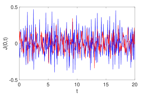
Figure 1: (Color online) Total current at the vertex for the boundary conditions (15) (blue) and (16) (red) as a function of time (for ).

It is clear that the norms of the eigenfunctions given by Eqs.(18) and (19) are positively defined. Direct numerical computation of the roots of Eq.(17) shows that they are indeed real. This implies that the eigenvalues of Eq.(1) for the boundary conditions (15) and (16) are real. Unlike Hermitian quantum graphs (see, e.g. Refs.Kost ; Uzy1 ; Uzy2 ; Exner15 ), the boundary conditions given by Eqs.(15) and (16) do not provide Kirchhoff rules. This implies breaking of the current conservation at the branching point that can be directly checked by computing numerically total current at the vertex ($x=0$) given by

$$J(0,t)=J_{1}(0,t)+J_{2}(0,t)+J_{3}(0,t),$$

where

$$J_{j}(0,t)=\frac{i}{2}[\psi_{j}(0,t)\partial_{x}\psi_{j}^{*}(0,t)-\partial_{x}\psi_{j}(0,t)\psi_{j}^{*}(0,t)],$$

is the current on each bond and

$$\psi_{j}(x,t)=\underset{n}{\sum}C_{n}e^{-ik_{n}^{2}t}\phi_{j}(x,k_{n}).$$

In Fig. 1 the total current at the vertex, $J(0,t)$ for the boundary conditions (15) and (16) are plotted as a functions of time. It is clear that current conservation (Kirchhoff rule) is broken.
Experimental realization on branched optical waveguides. Some models for PT-symmetric networks have been discussed earlier in the literature PTSN1 ; PTSN2 . However, the above model of the PT-symmetric quantum graph can be easily realized using branched (Y-junction) optical waveguides which are connected according to the boundary conditions given by Eqs. (15) or (16). It is clear that both set of boundary conditions provide absence of current at the end of the branches and the continuity of the wave function at the branching point. Taking into account breaking of Kirchhoff rules in these boundary conditions, one may construct such PT-symmetric quantum graph by connecting three optical wave guides via the small-size partially absorbing optical material. The ends of the branches of of the waveguides should provide total reflection of the wave. Similarly, one may consider experimental realization in general (more than three branched) star graph of optical waveguides and arbitrary graph topology such us, e.g. tree, loop and complete graphs. In this case all the branching points should be optically absorbing material, while the edge branches should provide zero-current at the ends. One of the options for dissipatively coupled optical waveguides have been recently discussed in Mukherjee . Different branched versions of such system can be also good candidate for PT-symmetric quantum graph.
Conclusions. We have studied the problem called “PT-symmetric quantum graphs” which represents branched quantum wires, whose branches are connected according to PT-symmetric rules. The latter implies that the boundary condition at the branching points and ends of the bonds provide PT-symmetry of the Schrödinger operator on a graph. General boundary conditions providing PT- symmetry of the Schrödinger operator on a graph and having real eigenvalues, as well as positively defined norm of the eigenfunctions are derived. Special types of the boundary conditions following from such conditions are presented. It is shown that the eigenvalue spectrum of the Schrödinger equation on metric graphs for such boundary conditions is real. Experimental realization of PT-symmetric quantum graph using branched optical waveguides is discussed. The above approach used for constructing PT-symmetric quantum star graph is applicable for other graph topologies, such us tree graph, loop graph, different fractal graphs, etc. Also, extension to the relativistic case can be easily done for PT-symmetric Dirac and Klein-Gordon equations on metric graphs.
Acknowledgements. We thank Carl M. Bender for his valuable comments on the paper. This work is partially supported by a grant of the Ministry of Innovation Development of Uzbekistan (Ref. No. F-2-003).

References

- (1) C. M. Bender and S. Boettcher, Phys. Rev. Lett. 80, 5243 (1998).
- (2) C. M. Bender and S. Boettcher, P. N. Meisinger, J. Math.Phys. 40, 2201 (1999).
- (3) C. M. Bender, S. Boettcher, and V.M. Savage, J. Math. Phys. 41, 6381(2000).
- (4) C. M. Bender and Q. Wang, J. Phys. A 34, 3325 (2001).
- (5) C. M. Bender, D. C. Brody, and H. F. Jones, Phys. Rev. Lett. 89, 270401 (2002).
- (6) C. M. Bender, S. Boettcher, P. N. Meisinger, and Q. Wang, Phys. Lett. A 302, 286 (2002).
- (7) C. M. Bender, D. C. Brody, and H. F. Jones, Am. J. Phys. 71, 1095 (2003).
- (8) C .M. Bender, D. C. Brody, and H. F. Jones, Phys. Rev. Lett. 93, 251601 (2004).
- (9) C. M. Bender, J. H. Chen, K. A. Milton, J. Phys. A 39, 1657 (2006).
- (10) C. M. Bender, Rep. Prog. Phys. 70, 94 (2007).
- (11) C. M. Bender, D. W. Hook, J. Phys. A 41, 392005 (2008).
- (12) C. M. Bender, P. D. Mannheim, Phys. Rev. D 78, 025022 (2008).
- (13) C. M. Bender, P. D. Mannheim, Phys. Lett. A 374, 1616 (2010).
- (14) S. Schindler and C. M. Bender, J. Phys. A 51, 055201 (2018).
- (15) C.M. Bender , C. Ford, N. Hassanpour and B. Xia, J. Phys. Commun. 2, 025012 (2018).
- (16) A. Mostafazadeh, J. Math. Phys. 43, 205 (2002).
- (17) A. Mostafazadeh, J. Phys. A 36, 7081 (2003).
- (18) A. Szameit, M. C. Rechtsman, O. Bahat-Treidel, and M. Segev, Phys. Rev. A 84, 021806(R) (2011).
- (19) O. Yeseiltas, J. Phys. A 46, 015302 (2013).
- (20) Y. X. Zhao, Y. Lu, Phys. Rev. Lett. 118, 056401 (2017).
- (21) M. Znojil, Can. J. Phys. 90, 1287 (2012).
- (22) M. Znojil, Can. J. Phys. 93, 765 (2015).
- (23) A. Dasarathy, J. P. Isaacson, K. Jones-Smith, J. Tabachnik, and H. Mathur, Phys. Rev. A 87, 62111 (2013).
- (24) El-Ganainy, R., K. G. Makris, D. N. Christodoulides, and Z. H. Musslimani, Opt. Lett. 32, 2632 ( 2007).
- (25) Ch. E. R ter, K. G. Makris, R. El-Ganainy, et.al., Nat. Phys. 6, 192 (2010).
- (26) A. A. Zyablovsky, A. P. Vinogradov, A. A. Pukhov, A. V. Dorofeenko, A. A. Lisyansky, Phys. Uspekhi 57, 1063 (2014).
- (27) V. V. Konotop, J. Yang, D. A. Zezyulin, Rev., Mod. Phys. 88, 035002 (2016).
- (28) J. Cuevas-Maraver, P. G. Kevrekidis, A. Saxena, F. Cooper, A. Khare, A. Comech, and C. M. Bender, J. Select. Topics in Quant. Electronics, 22, 7293090 (2016).
- (29) M. Chitsazi, H. Li, F. M. Ellis, and T. Kottos, Phys. Rev. Lett. 119, 093901 (2017).
- (30) S. Longhi, Phys. Rev. A 95, 012125 (2017).
- (31) P. Kurasov, B. Garjani, J. Math. Phys. 58, 023506 (2017).
- (32) M. Astudillo, P. Kurasov, M. Usman, Adv. Math. Phys. 2015 649795 (2015).
- (33) P. Exner, P. Seba, P. Stovicek, J. Phys. A 21 4009 (1988).
- (34) V. Kostrykin and R. Schrader J. Phys. A 32 595 (1999)
- (35) J. Bolte and J. Harrison, J. Phys. A 36 L433 (2003).
- (36) T. Kottos and U. Smilansky, Ann. Phys. 76 274 (1999).
- (37) S. Gnutzmann and U. Smilansky, Adv. Phys. 55 527 (2006).
- (38) P. Kuchment, Waves in Random Media 14 S107 (2004).
- (39) D. Mugnolo. Semigroup Methods for Evolution Equations on Networks. Springer-Verlag, Berlin, (2014).
- (40) G. Berkolaiko, P. Kuchment, Introduction to Quantum Graphs, Mathematical Surveys and Monographs AMS (2013).
- (41) P. Exner and H. Kovarik, Quantum waveguides. (Springer, 2015).
- (42) Oleh Hul et al, Phys. Rev. E 69, 056205 (2004).
- (43) K. K. Sabirov, Z. A. Sobirov, D. Babajanov, and D. U. Matrasulov, Phys. Lett. A 377, 860 (2013).
- (44) Z. Sobirov, D. Babajanov, D. Matrasulov, K. Nakamura, and H. Uecker, EPL.115 , 50002 (2016).
- (45) K. K. Sabirov, S. Z. Rakhmanov, D. U. Matrasulov and H. Susanto, Phys. Lett. A 382, 1092 (2018).
- (46) M. Christandl, N. Datta, A. Ekert, and A. J. Landahl, Phys. Rev. Lett. 92, 187902 (2004).
- (47) X. Z. Zhang, L. Jin, and Z. Song, Phys. Rev. A 85, 012106 (2012).
- (48) S. Mukherjee, D. Mogilevtsev, G. Ya. Slepyan, T. H. Doherty, R. R. Thomson, N. Korolkova, Nature Commun. 8, 1909 (2017).