Assessment of continuous and discrete adjoint method for sensitivity analysis in two-phase flow simulations
Abstract
Verification, validation and uncertainty quantification (VVUQ) have become a common practice in thermal-hydraulics analysis. An important step in the uncertainty analysis is the sensitivity analysis of various uncertainty input parameters. The efficient method for computing the sensitivities is the adjoint method. The cost of solving an adjoint equation is comparable to the cost of solving the governing equation. Once the adjoint solution is obtained, the sensitivities to any number of parameters can be obtained with little effort. There are two methods to develop the adjoint equations: continuous method and discrete method. In the continuous method, the control theory is applied to the forward governing equation and produces an analytical partial differential equation for solving the adjoint variable; in the discrete method, the control theory is applied to the discrete form of the forward governing equation and produces a linear system of equations for solving the adjoint variable. In this article, an adjoint sensitivity analysis framework is developed using both the continuous and discrete methods. These two methods are assessed with the one transient test case based on the BFBT benchmark. Adjoint sensitivities from both methods are verified by sensitivities given by the perturbation method. Adjoint sensitivities from both methods are physically reasonable and match each. The sensitivities obtained with discrete method is found to be more accurate than the sensitivities from the continuous method. The continuous method is computationally more efficient than the discrete method because of the analytical coefficient matrices and vectors. However, difficulties are observed in solving the continuous adjoint equation for cases where the adjoint equation contains sharp discontinuities in the source terms; in such cases, the continuous method is not as robust as the discrete adjoint method.
keywords:
sensitivity analysis , discrete adjoint method , continuous adjoint method , transient two-phase flow1 Introduction
In recent years, verification, validation and uncertainty quantification (VVUQ) have become a common practice in thermal-hydraulics analysis. In general, these activities deal with propagation of uncertainties in computer code simulations, e.g., through system analysis codes. An important step in uncertainty analysis is the sensitivity analysis of various uncertain input parameters. The common method to calculate sensitivity includes variance-based and regression-based methods. However, these methods require solving the system of interest multiple times, sometimes 100s of times, which is computationally expensive. An alternative method for calculating sensitivities is the adjoint method. The cost of solving an adjoint equation is comparable to the cost of solving the governing equation (forward equation, e.g. the two-phase two-fluid model). However, once the adjoint solution is obtained, the sensitivity to an arbitrary number of parameters can be calculated at the same time.
Adjoint equations are not rare throughout mathematics and its applications. There is a long history of using the adjoint method in optimal control theory. The use of adjoint method for computing sensitivities came up in the nuclear industry in the 1940s for the estimation of first eigenvalues of the transport equation. Later, the adjoint method became popular in computational fluid dynamics field [1, 2]. Within the field of aeronautical computational fluid dynamics, the use of adjoint method has been seen in [3, 4, 5, 6]. Adjoint problems arise naturally in the formulation of methods for optimal aerodynamic design and optimal error control [7, 2, 8, 9]. Adjoint solution provides the linear sensitivities of an objective function (e.g. lift force and drag force) to a number of design variables. These sensitivities can then be used to drive an optimization procedure. In a sequence of papers, Jameson developed the adjoint method for the potential flow, the Euler equation, and the Navier-Stokes equation [3, 4, 5, 6]. The application of the adjoint method to optimal aerodynamic design is very successful. However, to the author’s best knowledge, successful adjoint sensitivity analysis to two-phase flow problems is rare. Cacuci performed an adjoint sensitivity analysis to two-phase flow problems using the RELAP5/MOD3.2 numerical discretization [10, 11, 12]. An application of Cacuci’s method was illustrated by [13], where the method was applied to the blow-down of a gas from a pressurized vessel.
There are two methods to develop the adjoint equations: continuous and discrete [14]. In the continuous method, the control theory is applied to the governing equation through a variation analysis. The variation of the governing equation and the response function with respect to the primitive variables (e.g. pressure and velocity) and input parameters (e.g. boundary conditions) are combined through the use of Lagrange multipliers (adjoint variables). The continuous adjoint equation and its boundary conditions are specified by collecting the terms associated with the variation of the primitive variables; while the sensitivity is specified by the terms associated with the variation of the input parameters. The continuous adjoint equation is then discretized to obtain numerical solutions. In the discrete method, the control theory is applied directly to the discrete form of the governing equation (e.g. the residual vector given by the discretization). The discrete adjoint equation is specified by collecting terms associated with the variation of the primitive variables; while the sensitivity is specified by collecting terms associated with the variation of the input parameters. The discrete adjoint equation is usually given in the form of a system of linear equations.
The main advantage of the continuous adjoint method is that it provides a continuous adjoint equation in an analytical form, which does not depend on the solver for the forward equation and can be solved separately. This analytical form helps researchers study and understand the nature of the equation. The main disadvantage of the continuous method is that it requires one to develop an appropriate algorithm to discretize the adjoint equation and its boundary conditions. The development, verification, and validation of the adjoint code is complicated due to the lack of suitable benchmark test cases. The main advantage of the discrete adjoint method is that the code development is a straightforward process because it is closely related the forward solver. The variation of the discrete forward equations produces the coefficient matrices and vectors for the discrete adjoint equation. These coefficient matrices and vectors can be obtained either manually or by automatic differentiation. The robustness and accuracy of the adjoint code is the same as that of the forward code because the eigenvalues of the two systems are the same. The main disadvantage of the discrete method is the extra complexity in obtaining coefficient matrices/vectors manually or the extra cost in obtaining coefficient matrices/vectors with automatic differentiation.
In previous work [15, 16, 17], the author applied separately the continuous and adjoint methods to sensitivity analysis in steady-state two-phase flow simulations. Both methods were found to work well. However, these two methods were based on different forward solver and were assessed with different test problems. This article will assess both methods within the same framework for a consistent comparison. In additions, the previous studies were limited to steady-state problems. Since the transient behavior of the two-phase system is important in reactor safety analysis, this article will assess the application of both continuous and adjoint methods to sensitivity analysis in transient two-phase flow simulations.
This article is organized in the following way. Section 2 presents briefly the forward numerical scheme for solving the two-phase two-fluid model equation. Section 3 presents the adjoint sensitivity analysis framework for both continuous and discrete adjoint method for transient two-phase flow simulations. Section 4 presents the numerical tests for verification and assessment of both continuous and discrete adjoint methods. The faucet flow will be used to assess the application of both methods to steady-state problems. One transient test in BFBT benchmark will be used to assess the application of both methods to realistic transient two-phase flow problems. Section 5 presents the conclusion and the future work of the current adjoint sensitivity analysis framework.
2 Forward solver
2.1 Two-phase two-fluid model
For 1D problems, the basic two-phase two-fluid six-equation model without any differential closure correlations [18] can be written in a vector form as
| (1) |
where is the vector of conservative variables, is the vector of flux variables, and are the vectors related to the partial derivatives of the void fraction, and is the vector of source terms. They are defined as
| (2) |
Let the subscript denote the liquid phase and gas phase, respectively. The variables denote the volume fraction, the density, the velocity, and the specific internal energy of -phase. The summation of phasic volume fraction should be one, i.e. . is the pressure of two phases. and are the phasic specific total energy and specific total enthalpy.
An appropriate Equation of State (EOS) is required to close the system. For many practical problems in the nuclear thermal-hydraulics analysis, the temperature of two phases are required to model the source terms. In such a case, a useful EOS is given by specifying the Gibbs free energy as a function of pressure and temperature , i.e.
| (3) |
After specifying the specific Gibbs free energy, the phasic density and specific internal energy are obtained from the partial derivatives of the specific Gibbs free energy. The details about specifying the EOS through the specific Gibbs free energy are referred to [19, 15].
2.2 Numerical scheme
For 1D problems, the spatial discretization is shown schematically in Figure 1. The physical domain is divided into cells. The cell center is denoted with an index and the cell boundaries are denoted with , for . All unknown variables are solved in the cell center (co-located mesh). On each side of the physical domain, ghosts cells are used to deal with boundary conditions.

The two-phase two-fluid model is solved with the backward Euler method, which gives a fully implicit scheme
| (4) |
where is an operator representing the spatial differential operators and the source terms,
| (5) |
where and are low-order numerical fluxes at cell boundaries. More details of the numerical scheme can be seen in [20].
A first-order Roe-type numerical flux is constructed following the Roe-Pike [21, 22] method. Let be the Jacobian matrix defined as . The subscript denotes that the Jacobian matrix and eigenvalues/eigenvectors are obtained with the conservative part of the equation [23, 15]. Let and , for be the eigenvalues and right eigenvectors of the matrix . Let be a scalar function defined as
| (6) |
where is the coefficient for the addition of numerical viscosity term, which is set at 0.125 as was used by Yee [24]. The Roe-type numerical flux is constructed by
| (7) |
where is the wave strength when projecting the conservative vectors to the characteristic space. The Jacobian matrix, approximate eigenvalues, and eigenvectors are given in the Appendix A for reference. Complete details about the approximate eigenvalues/eigenvectors and the average state are referred to [23, 15].
Eq. (4) forms a set of algebraic nonlinear equations, which are solved with the JFNK method. Eq. (4) can be generalized as
| (8) |
where denotes the global residual function of Eq. (4) and is the vector of unknown primitive variables. The JFNK method is based on the Newton’s method, which solves the nonlinear algebraic equations iteratively
| (9) | ||||
| (10) |
where denotes the -th step of the iteration. The iteration starts with an initial guess of which is usually taken from the old time step. is the Jacobian matrix define as
| (11) |
In the JFNK scheme, the linear equation Eq. (9) is solved with the Krylov subspace method. The essential idea of the JFNK method is that the Krylov method requires only the matrix-vector product and the explicit form of the Jacobian matrix could be avoided. The matrix-vector project is approximated with
| (12) |
where is the Krylov vector and is a small parameter. In this article, the JFNK method is implemented with the scientific computational toolkit PETSc [25].
3 Adjoint sensitivity analysis
3.1 General framework
Let be the operator that represents the governing equation of the forward problem, e.g. the two-phase two-fluid equation. Let be the vector of physical variables. For the forward problem, there are usually a few parameters () that affect the solution, e.g. the physical model parameters and boundary conditions. Suppose the governing equation is written as
| (13) |
Let be the operator that measures the quantity of interest (response function), e.g. void fraction. The response could be expressed as
| (14) |
In the following discussion, vectors and matrices are defined in a way such that the multiplications shown in the following equations are the inner product.
Let be the variation operator. A perturbation in the parameter of interest, , will cause
| (15) |
| (16) |
Note that is the sensitivity we would like to quantify. Solving for with Eq. (15) is usually expensive because it requires solving the forward problems. The idea of the adjoint method is to remove the dependency of on by combining Eq. (15) and Eq. (16) using Lagrange multipliers.
For brevity, the subscripts and in the partial derivatives are dropped. Let be a vector of free variables which represents the vector of Lagrange multipliers. Multiplying the transpose of the Lagrange multiplier to Eq. (15) gives
| (17) |
where the superscript denotes the transpose operator. Since the right-hand side of Eq. (17) is zero, Eq. (17) can be subtracted from Eq. (16) without changing the value of , i.e.
| (18) |
Eq. (18) is rewritten as
| (19) |
Because the Lagrange multiplier is a vector of free variables, it can be chosen in a way such that
| (20) |
The so-called adjoint equation is obtained by taking the transpose of Eq. (20), i.e.
| (21) |
The Lagrange multiplier given by Eq. (21) is the so-called adjoint variable. With Eq. (21), the sensitivity is obtained with
| (22) |
Note that if the response function does not depend explicitly on , then can be removed from Eq. (22). The advantage of Eq. (22) is that it is independent of , which means that the sensitivity of the response to an arbitrary number of parameters can be determined without the need for additional forward calculations.
3.2 Application of continuous adjoint method to two-fluid model
3.2.1 Continuous adjoint equation
The adjoint equation Eq. (21) and the response equation Eq. (22) are problem dependent. The continuous adjoint method works with the PDE of the forward problem, i.e. Eq. (1). Note that the term term can be handled by the matrix , i.e.
| (23) |
Because and its inverse can be obtained analytically, its effect can be considered later if interested. The derivation is started with
| (24) |
Let denote the integration in space, denote the integration in time, and denote the double integration in space and time. The integration in time is from to time and the integration in space is from to . In this article, the response function is generalized as
| (25) |
where is the quantity of interest which is a function of the primitive variables (). Applying the variation operator to the response function gives,
| (26) |
Let be the Lagrange multiplier (the adjoint variable). Multiplying to the variation of Eq. (24) and integrating the product over space and time gives
| (27) |
where the following matrices are defined
| (28) |
Note that the effect of term can be added to . Subtracting Eq. (27) from Eq. (26) gives
| (29) |
The continuous adjoint equation is obtained with Eq. (29) by removing the dependency of part on unknown , i.e.
| (30) |
The ICs for Eq. (30) is obtained by by removing the dependency of part on unknown , i.e.
| (31) |
The BCs for Eq. (30) are obtained by removing the dependency of part on unknown , i.e.
| (32a) | ||||
| (32b) | ||||
where to are functions of that results from . Details of to are given in the Appendix B. Complete details for obtaining Eq. (30), Eq. (31), and Eq. (32) are referred to [15].
Substituting Eq. (30), Eq. (31), and Eq. (32) into Eq. (29), the variation in the response function is reduced to
| (33) |
Sensitivities of the response function to source parameters, boundary conditions, and initial conditions can be obtained with the first, second, and third part of the right hand side of Eq. (33), respectively. In the following analysis, the sensitivity obtained with the continuous adjoint method is denoted as ‘CAS’.
The same mesh, Figure 1, will be used to solve the adjoint equation. A central finite difference discretization will be used, which works well for problems where the forward solution is smooth, see [16]. Eq. (30) is discretized as
| (34) |
where the superscript denotes the time step. Note that Eq. (31) shows that the adjoint equation has to start from the end time () and integrate back to the start time , thus Eq. (34) will be assembled to a global linear equation for solving at step .
3.3 Application of discrete adjoint method to two-fluid model
The derivation of discrete adjoint equation starts with the discrete form of the forward problem, i.e. Eq. (4). For the time step, The discrete form of Eq. (1) can be summarized as
| (35) |
where is the total number of time steps. Considering Eq. (35) in all cells and the input parameters (), the discretized forward equation at time step can be generalized as
| (36) |
where and is the global residual and solution vector at step, respectively. There are in total steps. Let be the global residual vector assembled with for all steps, i.e.
| (37) |
This way, the discrete form of the forward problem is specified by
| (38) |
where represents the vector of forward solution at all time steps and all cells.
The response function for the discrete adjoint problem can be generalized as
| (39) |
where is a scalar function of the solution vector .
Let be the adjoint solution at the step and be the global adjoint solution assembled from all time step, i.e.
| (40) |
The discrete adjoint equation is obtained by assigning to the operator and to the operator in Eq. (21), i.e.
| (41) |
and the sensitivity is given as
| (42) |
Because the effect of ICs and BCs has already been included in the residual vector , Eq. (41) and Eq. (42) haven o explicit dependency on ICs and BCs. In the following analysis, the sensitivity obtained with the discrete adjoint method is denoted as ‘DAS’.
The number of time steps for a transient problem may be very large, the dimension of Eq. (41) is too large to solve efficiently . Fortunately, because the temporal discretization of the forward problem involves only forward solution at two steps, Eq. (41) can be split into a series of linear equations with a smaller dimension. It is found that the coefficient matrix/vector in Eq. (41) has the following form
| (43) |
Thus, the adjoint variable can be solved with
| (44) |
In practice, the coefficient matrices and vectors in Eq. (44) are obtained with a numerical differentiation scheme. After obtaining the adjoint variable, the sensitivity can be obtained with
| (45) |
Because the forward discretization is upwind and the coefficient matrices for the DAS is the transpose of the forward Jacobian matrices, the solver for solving the discrete adjoint equation behaves like the forward solver. In other words, if the forward solver is stable and robust, the discrete adjoint solver is also stable and robust. This is a critical feature of the discrete adjoint method.
3.4 Steady-state problems
3.5 Response function
The form of the response function does not affect the application of the adjoint method and should depend on different problems. This article considers a group of response function that can be written as
| (46) |
where is the total number of cells, is the total number of time steps, is the location of the cell, and denotes a function of the primitive variable, e.g. . The other variable, , is a weight function which is used to study the behavior of the response function at different location and time . The dependency of the response function on and is designed for verification purposes. In this study, is non-zero only in the neighboring cells of and at time step , which simulates a point-wise response function. The adjoint sensitivity analysis is in general efficient for problems with few response functions.
The sensitivity coefficient is used for comparison. The sensitivity coefficient is defined as
| (47) |
where and are the nominal values of the input parameter and response, respectively.
3.6 Perturbation sensitivity analysis
It is in general impractical to get exact sensitivities to verify the sensitivities obtained with the adjoint method. A perturbation analysis is used to provide the reference value of the sensitivities. The procedure for the perturbation sensitivity analysis is straightforward,
| (48) |
where denotes the sensitivity from perturbation sensitivity analysis, and are the response functions calculated by performing the forward simulation with and without the perturbation to the input parameter of interest, respectively. In practice, is used.
4 Numerical tests
4.1 Steady-state test with faucet flow
This test is the Ransom’s faucet flow problem [26, 27, 28, 29], which has an analytical solution. This test problem consists of a liquid stream entering a vertical tube at the top and falling under gravity to form a liquid stream of decreasing cross-section. The length of the vertical tube is m. The boundary conditions are: , K, K, m/s, m/s, and MPa. Properties of liquid and gas are obtained from the IAPWS-IF97 formulation [19]. Since there is no mass and heat transfer between the liquid and gas phases, the superheated steam is used to simulate the gas phase. The source vector of this problem is
| (49) |
where is the gravitational acceleration constant and the superscript is the transpose operator.
The void fraction, liquid velocity, and pressure are of particular interest to this test. The steady-state solution [27, 30] of this problem is
| (50) | ||||
| (51) | ||||
| (52) |
where is the gravitational acceleration constant and is
| (53) |
where and .
4.1.1 Input parameters
For this test, 3 input parameters are considered: inlet void fraction, inlet liquid velocity, and gravitational constant, i.e.
| (54) |
The inlet void fraction and inlet liquid velocity represent typical input parameters related to boundary conditions; while the gravitational constant represent typical input parameters in the source terms. Several sensitivities can be obtained analytically, i.e.
| (55) |
These analytical sensitivities are used to verify the adjoint sensitivity analysis framework by studying the estimation error in the continuous and discrete adjoint sensitivity analysis.
4.1.2 Results
The forward solver is at first run to reach steady-state for preparing the coefficient matrices/vectors. Numerical solutions match the analytical solution well. Assessment of the forward solver is omitted in this article and is referred to [20]. For this test, and 11 points () are used. At first, a mesh convergence study is done to select an appropriate mesh size, shown in Figure 2. It is seen that is fine enough for the sensitivity analysis, which is used in the following analysis. Then both continuous and discrete adjoint method are applied to calculate the sensitivities given in Eq. (55). The estimation error for the sensitivities from both methods is listed in Table 1. It is seen that both continuous and discrete adjoint methods calculate the sensitivities very well. From the comparison, it is seen that the continuous adjoint method tends to give more accurate sensitivities than the discrete adjoint method. The explanation is that the coefficient matrix is approximated with a finite difference method in the discrete adjoint method; while the coefficient matrix is given analytically in the continuous adjoint method. Because of the extra effort to compute the coefficient matrix with a finite difference method, the discrete adjoint method takes more computational time than the continuous adjoint method.
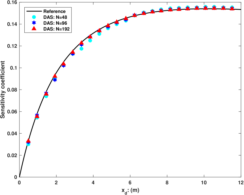
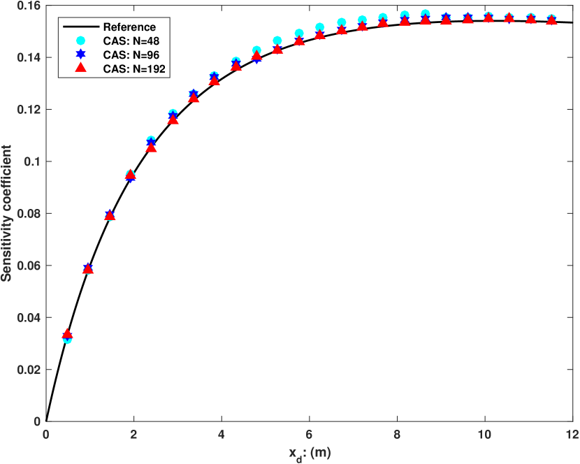
| REF | : % | : % | REF | : % | : % | REF | : % | ||
| :(m) | |||||||||
| 0.96 | 9.17E-01 | 0.94 | -0.03 | -1.16E-01 | -5.47 | -10.48 | 5.82E-02 | -4.60 | -0.40 |
| 1.92 | 8.52E-01 | 0.89 | -0.24 | -1.87E-01 | -1.99 | -4.05 | 9.33E-02 | -1.25 | 1.55 |
| 2.88 | 7.99E-01 | 1.12 | 0.68 | -2.31E-01 | -1.92 | -0.97 | 1.15E-01 | -1.28 | 0.05 |
| 3.84 | 7.55E-01 | 1.25 | 0.17 | -2.60E-01 | -1.66 | -2.62 | 1.30E-01 | -1.09 | 0.55 |
| 4.80 | 7.18E-01 | 1.02 | -0.01 | -2.78E-01 | -1.02 | -1.80 | 1.39E-01 | -0.50 | 0.82 |
| 5.76 | 6.85E-01 | 1.10 | 0.56 | -2.91E-01 | -0.91 | -0.64 | 1.45E-01 | -0.43 | 0.28 |
| 6.72 | 6.57E-01 | 1.02 | 0.36 | -2.99E-01 | -0.69 | -0.48 | 1.49E-01 | 0.20 | 0.37 |
| 7.68 | 6.32E-01 | 1.04 | 0.11 | -3.04E-01 | -0.61 | -1.14 | 1.52E-01 | 0.19 | 0.59 |
| 8.64 | 6.09E-01 | 1.06 | 0.50 | -3.06E-01 | -0.52 | -0.48 | 1.53E-01 | 0.20 | 0.26 |
| 9.60 | 5.89E-01 | 0.86 | 0.34 | -3.08E-01 | -0.42 | -0.44 | 1.54E-01 | 0.23 | 0.26 |
| 10.56 | 5.71E-01 | 0.89 | 0.18 | -3.08E-01 | -0.37 | -0.84 | 1.54E-01 | 0.23 | 0.45 |
| 11.52 | 5.54E-01 | 0.92 | 0.46 | -3.07E-01 | -0.31 | -0.41 | 1.54E-01 | 0.25 | 0.23 |
| :(m) | |||||||||
| 0.96 | 9.17E-01 | 0.73 | 0.82 | 8.64E-02 | -5.04 | -3.30 | -4.71E-04 | 1.96 | -0.89 |
| 1.92 | 8.52E-01 | 0.68 | 0.63 | 1.61E-01 | -1.29 | 0.26 | -4.30E-04 | 1.67 | -0.83 |
| 2.88 | 7.99E-01 | 0.96 | 0.30 | 2.26E-01 | -1.71 | 0.31 | -3.89E-04 | 1.97 | 0.13 |
| 3.84 | 7.55E-01 | 1.14 | 1.05 | 2.85E-01 | -1.80 | -0.78 | -3.48E-04 | 2.32 | -0.11 |
| 4.80 | 7.18E-01 | 0.96 | 0.88 | 3.38E-01 | -0.81 | 0.04 | -3.07E-04 | 1.88 | -0.60 |
| 5.76 | 6.85E-01 | 1.09 | 0.27 | 3.87E-01 | -0.97 | 0.14 | -2.66E-04 | 2.21 | -0.01 |
| 6.72 | 6.57E-01 | 0.95 | 0.06 | 4.33E-01 | -0.19 | 0.56 | -2.25E-04 | 1.49 | -0.80 |
| 7.68 | 6.32E-01 | 1.03 | 1.00 | 4.76E-01 | -0.38 | 0.01 | -1.84E-04 | 1.89 | -0.71 |
| 8.64 | 6.09E-01 | 1.10 | 0.19 | 5.16E-01 | -0.51 | 0.09 | -1.43E-04 | 9.67 | 0.07 |
| 9.60 | 5.89E-01 | 0.95 | 0.03 | 5.55E-01 | -0.18 | 0.37 | -1.02E-04 | 0.96 | -1.49 |
| 10.56 | 5.71E-01 | 1.02 | 1.07 | 5.91E-01 | -0.30 | -0.01 | -6.14E-05 | 1.84 | -1.05 |
| 11.52 | 5.54E-01 | 1.08 | 0.13 | 6.26E-01 | -0.41 | 0.06 | -2.05E-05 | 6.25 | 3.86 |
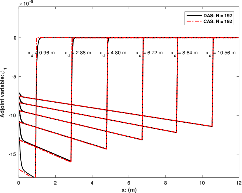
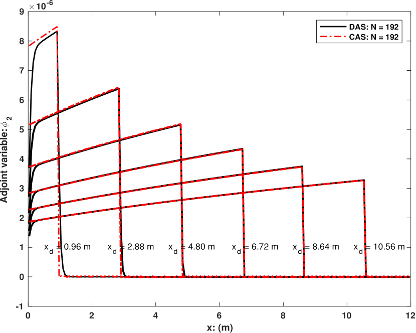
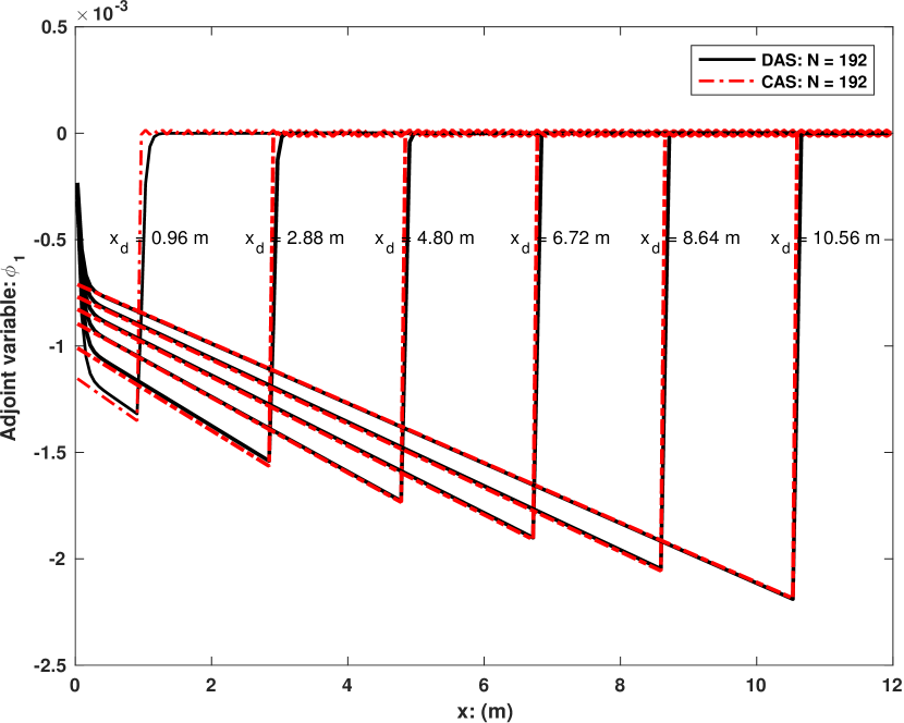
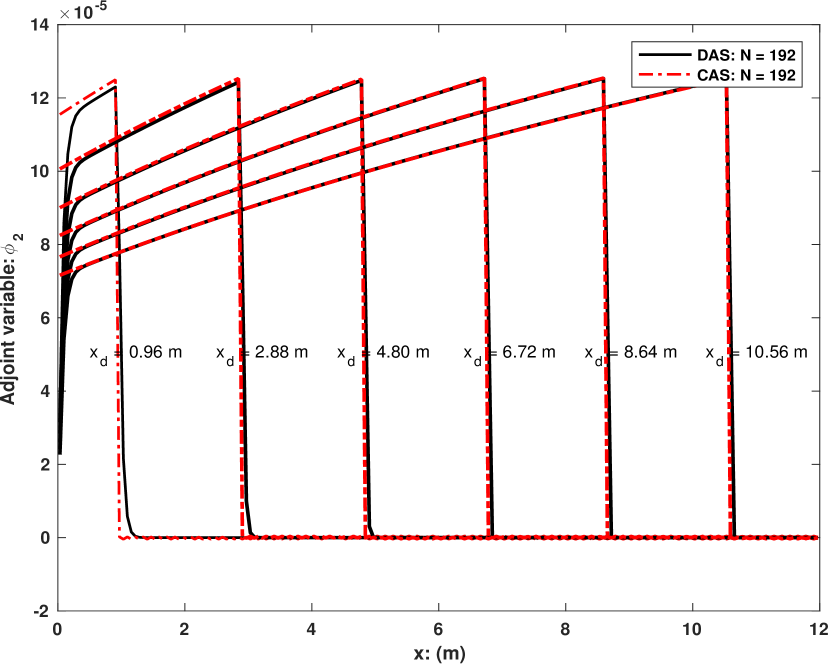
Figure 3 shows the adjoint variable components obtained from both continuous and discrete adjoint method. The adjoint variable component represents the effect (or value) of the respective forward governing equation to the response of interest, e.g. and represents the effect of the liquid mass and momentum equation, respectively. For this faucet flow problem, it is the liquid mass and momentum equation that affect the forward solution (and the response). The effect of the other 4 equations is negligible. The profile of the adjoint component is reasonable. For a response at a certain location (), we expect that the response is mainly affected by its upstream but not its downstream. The nonzero and zero magnitude of the adjoint component at the upstream and downstream, respectively, is consistent with this expectation. It is seen that the adjoint variable obtained from continuous and discrete adjoint method matches well except near the boundaries. This is reasonable. For the continuous adjoint method, the effect of boundary conditions is calculated by Eq. (33) (i.e. the variable), which depends only on the adjoint variable at the boundary. However, for the discrete adjoint method, the effect of boundary conditions is calculated by Eq. (42), which actually depends on both the boundary point and its neighbors because of the three-point stencil used in the forward numerical scheme.
4.2 Transient test with BFBT benchmark
One of the most valuable and publicly available databases for thermal-hydraulic modeling of Boiling Water Reactor (BWR) channels is the OECD/NEA BWR Full-size Fine-mesh Bundle Test (BFBT) benchmark, which includes sub-channel void fraction measurements in a full-scale BWR fuel assembly [31]. There are two types of void distribution measurement systems: an X-ray CT scanner and an X-ray densitometer [31]. There are 4 measurement locations, which are denoted by DEN #3 (0.682 m), DEN #2 (1.706 m), DEN #1 (2.730 m), and CT (3.708 m) starting from the bottom. The geometry and system configurations of the channel are shown in Table 2.
| Geometry parameters | System/experiment parameters | ||
|---|---|---|---|
| Heated length (m) | 3.708 | Pressure (MPa) | 3.9 - 8.7 |
| Width of channel box (m) | 0.1325 | Inlet temperature (∘C) | 238. - 292. |
| Hydraulic diameter (m) | 0.01284 | Inlet subcooling (kJ/kg) | 50. - 56. |
| Volumetric wall surface area () | 311.5 | Flow rate (t/h) | 10. - 70. |
| Flow area () | 9.463E-03 | Power (MW) | 0.62 - 7.3 |
| Wetted perimeter (m) | 3.003 | Exit quality (%) | 8. - 25. |
Closure correlations are required to simulate the behavior of a boiling system. For this type of problems, the source vector is modeled as
| (56) |
where is the net vapor generation rate due to near wall vapor generation () and bulk vapor generation (), is the interface velocity, is the interfacial friction, is the phasic wall friction, is the phasic interfacial heat flux, is the phasic wall heat flux, is the phasic enthalpy carried by the wall vapor generation term (), and is the phasic enthalpy carried by the bulk vapor generation term (). Correlations based on RELAP5-3D code manual [32, 33] are used to model these variables. Details of all physical models are provided in [23, 15].
The void fraction is the main response of interest in this test. The main physical model that affects the void fraction is the near wall vapor generation rate (), which is determined by the Lahey ([34]) model, i.e.
| (60) | ||||
| (61) |
where is the volumetric wall heat flux, is the volumetric wall surface area, is the specific saturation enthalpy of liquid phase, and is the difference between the liquid and gas phase specific saturation enthalpy. In case of the the subcooled boiling, the bulk liquid can be subcooled while liquid in the boundary layer is saturated and is flashing to vapor. Depending on the inlet subcooling level, the system may start from a liquid phase () and transits to two phases (). The condition for this transition is that the specific enthalpy of the liquid phase () is greater than a critical enthalpy . Passing this transition point, the void fraction begins to increase. Currently, the critical enthalpy () is modeled with the Saha-Zuber [33] correlation, i.e.
| (62) |
where is the Peclet number, is the Stanton number, and is the Nusselt number. More details are referred to [33].
4.3 Transient test problem
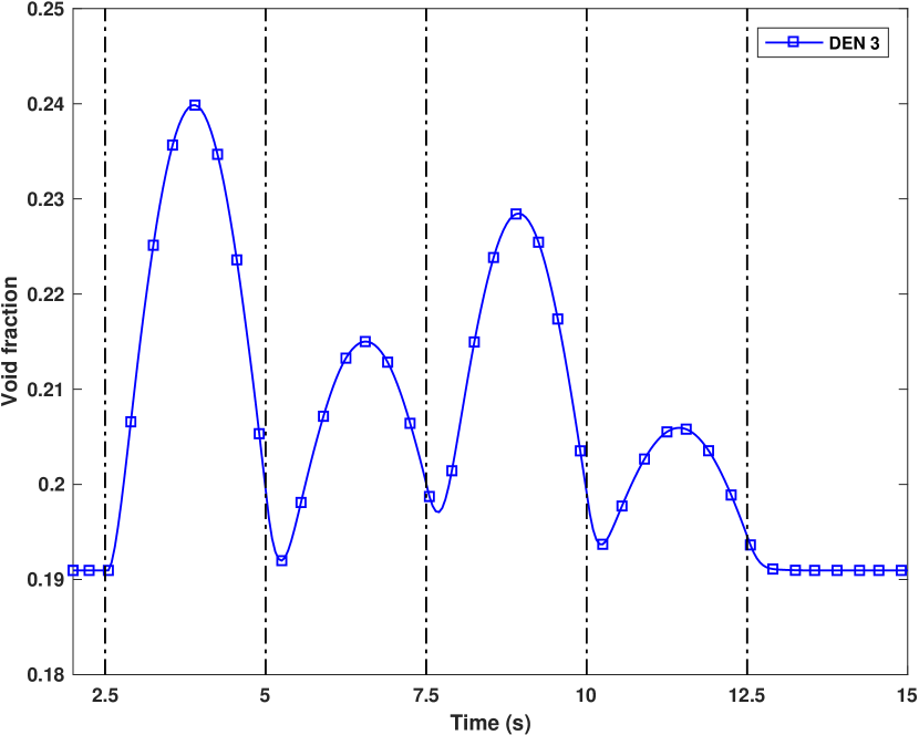
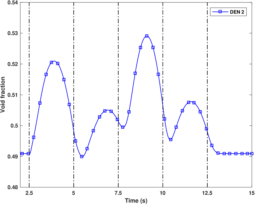
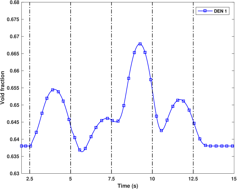
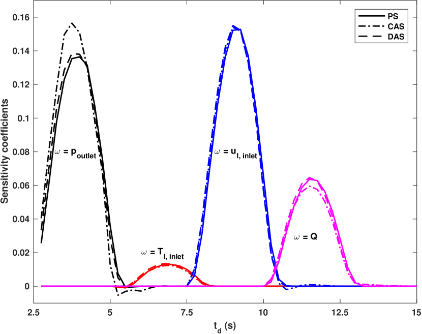
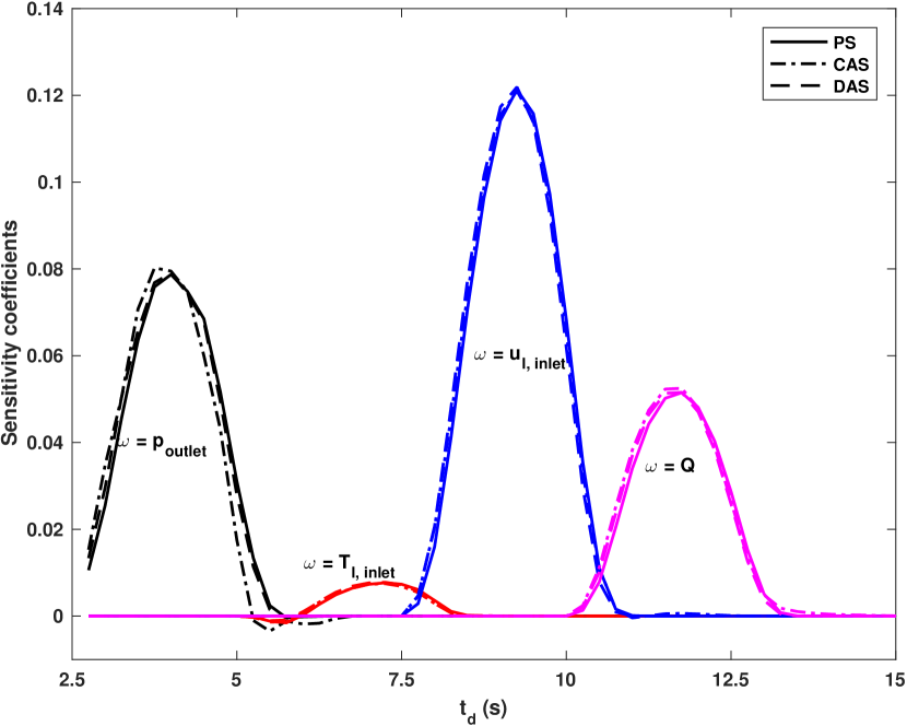
One transient test is designed for verification purposes. The test contains 4 transient period: outlet pressure () decrease transient (T1), inlet liquid temperature () increase transient (T2), inlet liquid velocity () decrease transient (T3), and assembly power () increase transient (T4). These 4 periods simulate the typical boundary conditions change in the boiling channel that cause a increase in the void fraction. For simplicity reasons, the boundary conditions are changed through
| (63) |
where denotes the start of the transient period, denotes the end of the transient period, denotes the boundary condition (e.g. ), denotes the value of at time , and is the change rate of . These values are listed in Table 3. The transient void fraction at 3 locations is shown in Figure 4. Both the forward and adjoint simulations will be performed with s and .
| Test period | |||||
|---|---|---|---|---|---|
| T1 | 2.5 s | 5.0 s | 7.12 MPa | -0.2 MPa | |
| T2 | 5.0 s | 7.5 s | 554.2 K | 1.0 K | |
| T3 | 7.5 s | 10.0 s | 2.069 m/s | -0.25 m/s | |
| T4 | 10.5 s | 12.5 s | 4.53 MW | 0.25 MW |
4.4 Input parameters
The input parameters should be chosen according to the specific purposes. For typical boiling problems, boundary conditions are usually specified by inlet liquid temperature, inlet liquid velocity, and outlet pressure; physical models are specified by net vapor generation rate (), interfacial friction (), wall friction (), interfacial heat flux (), and wall heat flux (). Many of these physical models are correlated, e.g. , , and are correlated through the interfacial heat transfer coefficients (). Excluding the wall heat flux, which is mainly affected by the assembly power, there are 5 independent physical models that worth studying in details, including , , , , and . In case of the subcooled boiling, the physical model for predicting the critical enthalpy () is worth studying, as it specifies the transition from single-phase to two-phase flow.
Sensitivity of the void fraction () to 11 parameters will be studied. These 11 parameters are
| (64) |
where is the hydraulic diameter, which represents the typical geometry parameter. A perturbation is required to calculate the coefficient matrices and vectors. The 4 boundary conditions are perturbed by the change rate, i.e.
| (65) |
where denotes the perturbation. The hydraulic diameter is perturbed by
| (66) |
The critical enthalpy is perturbed by
| (67) |
where and are the nominal values used by Eq. (62). The remaining 5 physical model parameters are perturbed by,
| (68) |
Perturbation in this form is mainly a numerical compromise to avoid messing with the existing closure correlations; however, it does not affect the application of the adjoint method to calculate the sensitivity. Note that is obtained directly from the existing closure correlations and remains unchanged.
4.5 Results
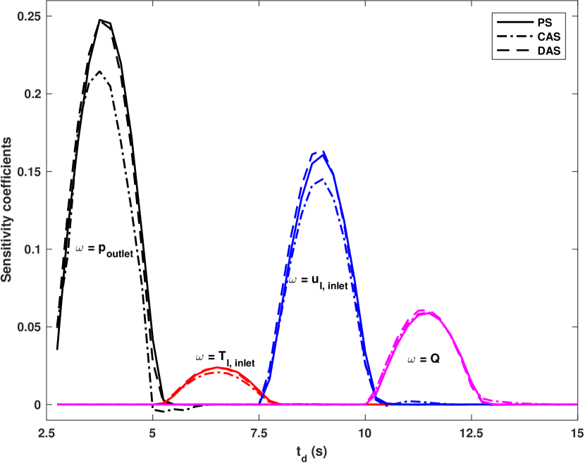
The response of interest is the void fraction at 3 locations (DEN 3, DEN 2, and DEN 1) and 50 time steps starting from 2.5 to 15.0 s. Sensitivities to all input parameters are calculated with perturbation sensitivity analysis (PS), continuous adjoint sensitivity analysis (CAS), and discrete adjoint sensitivity analysis (DAS). A large volume of the sensitivity result is generated. For brevity reasons, only a few series of the result will be shown quantitatively. The sensitive input parameters are the change rate of 4 boundary conditions.
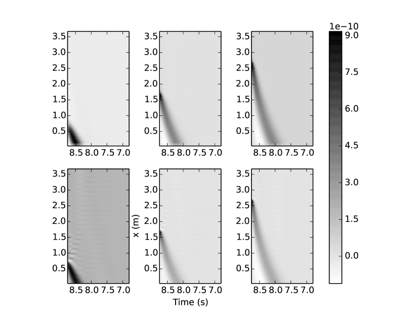
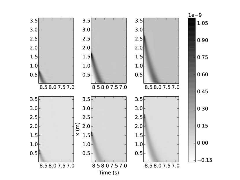
Figure 5, Figure 6, and Figure 7 show examples of the time and space dependent adjoint variables given by both CAS and DAS schemes. The void fraction at 3 locations and at s is the response of interest. The profile of the adjoint variables from CAS and DAS schemes are similar, which means that the CAS and DAS are consistent with each other. Vertically, it is seen that the adjoint variable is non-zero for but negligible for , which reflects that the response is mainly affected by forward solution in its upwind side. Horizontally, it is seen that when the time decreases, the adjoint variable decreases rapidly to 0, which reflects that the response is mainly affected by its prior but close state.
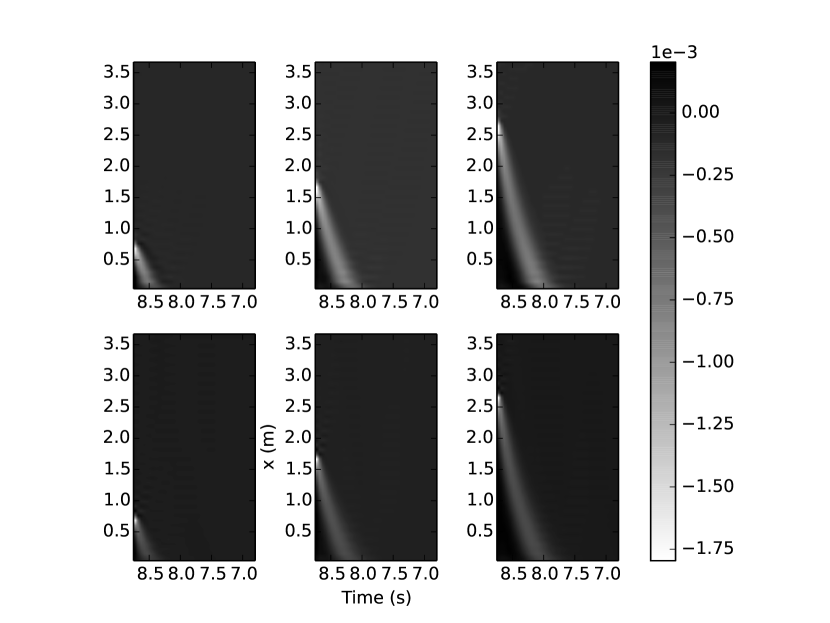
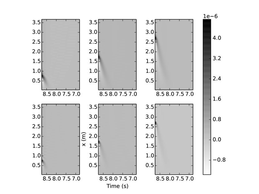
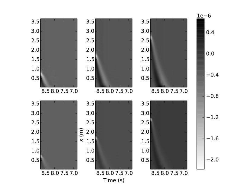
For clarity reasons, let’s denote adjoint variable with
| (69) |
In each time step, there are 6 components in the adjoint vector in each location. The component of the adjoint vector represents the effect of the corresponding governing equation, e.g. for the liquid mass equation, to the response. The notation in Eq. (69) represents the effect of the system at to the response of interest at .
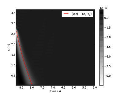
Let be the time period when is the biggest. There are 6 characteristic waves in the two-phase system, including both acoustic waves and the convection waves. Because the time step is too large to capture the the acoustic waves, the remaining important wave is the convection of liquid enthalpy, which has a wave speed of the liquid velocity. Thus, can be approximately by
| (70) |
Eq. (70) gives a curve in space that represents the location of the maximum adjoint solution, see Figure 8. The good agreement of this curve verifies the current adjoint sensitivity analysis framework.
| DEN 3 | DEN 2 | DEN 1 | |||||||
| :(s) | PS | CAS | DAS | PS | CAS | DAS | PS | CAS | DAS |
| 3.00 | 1.13E-01 | 9.60E-02 | 1.24E-01 | 6.10E-02 | 8.05E-02 | 7.02E-02 | 2.54E-02 | 3.47E-02 | 2.95E-02 |
| 3.50 | 2.20E-01 | 2.07E-01 | 2.26E-01 | 1.23E-01 | 1.50E-01 | 1.28E-01 | 6.35E-02 | 7.08E-02 | 6.58E-02 |
| 4.00 | 2.45E-01 | 2.05E-01 | 2.42E-01 | 1.36E-01 | 1.51E-01 | 1.38E-01 | 7.87E-02 | 7.95E-02 | 7.90E-02 |
| 4.50 | 1.72E-01 | 1.25E-01 | 1.64E-01 | 1.07E-01 | 9.75E-02 | 1.04E-01 | 6.85E-02 | 6.00E-02 | 6.78E-02 |
| 5.50 | 5.90E-03 | 6.22E-03 | 7.02E-03 | -9.76E-04 | -5.86E-04 | -6.88E-04 | -1.16E-03 | -1.07E-03 | -1.38E-03 |
| 6.00 | 1.89E-02 | 1.68E-02 | 1.95E-02 | 5.32E-03 | 5.88E-03 | 6.45E-03 | 1.92E-04 | 9.78E-04 | 7.65E-04 |
| 6.50 | 2.39E-02 | 2.09E-02 | 2.38E-02 | 1.14E-02 | 1.11E-02 | 1.23E-02 | 4.90E-03 | 5.06E-03 | 5.47E-03 |
| 7.00 | 2.08E-02 | 1.73E-02 | 2.01E-02 | 1.29E-02 | 1.24E-02 | 1.32E-02 | 7.33E-03 | 7.33E-03 | 7.64E-03 |
| 8.00 | 5.75E-02 | 5.52E-02 | 6.65E-02 | 3.20E-02 | 3.89E-02 | 4.04E-02 | 1.59E-02 | 2.04E-02 | 2.07E-02 |
| 8.50 | 1.33E-01 | 1.22E-01 | 1.41E-01 | 1.08E-01 | 1.13E-01 | 1.16E-01 | 7.08E-02 | 7.41E-02 | 7.74E-02 |
| 9.00 | 1.61E-01 | 1.45E-01 | 1.64E-01 | 1.52E-01 | 1.54E-01 | 1.55E-01 | 1.14E-01 | 1.15E-01 | 1.17E-01 |
| 9.50 | 1.19E-01 | 1.07E-01 | 1.16E-01 | 1.37E-01 | 1.33E-01 | 1.33E-01 | 1.16E-01 | 1.14E-01 | 1.14E-01 |
| 10.50 | 2.30E-02 | 2.67E-02 | 2.70E-02 | 1.48E-02 | 1.78E-02 | 1.87E-02 | 7.88E-03 | 1.12E-02 | 1.01E-02 |
| 11.00 | 5.06E-02 | 5.21E-02 | 5.42E-02 | 4.80E-02 | 4.78E-02 | 5.15E-02 | 3.40E-02 | 3.82E-02 | 3.69E-02 |
| 11.50 | 5.89E-02 | 5.94E-02 | 6.09E-02 | 6.37E-02 | 5.96E-02 | 6.47E-02 | 5.02E-02 | 5.23E-02 | 5.14E-02 |
| 12.00 | 4.53E-02 | 4.48E-02 | 4.48E-02 | 5.63E-02 | 5.04E-02 | 5.45E-02 | 4.81E-02 | 4.80E-02 | 4.71E-02 |
| DEN 3 | DEN 2 | DEN 1 | |||||||
| :(s) | PS | CAS | DAS | PS | CAS | DAS | PS | CAS | DAS |
| 3.75 | -1.96E-01 | -2.50E-01 | -2.06E-01 | -2.57E-01 | -2.43E-01 | -2.58E-01 | -2.19E-01 | -2.26E-01 | -2.20E-01 |
| 6.25 | -1.93E-01 | -2.59E-01 | -2.05E-01 | -2.80E-01 | -2.54E-01 | -2.82E-01 | -2.36E-01 | -2.44E-01 | -2.38E-01 |
| 8.75 | -2.08E-01 | -2.75E-01 | -2.23E-01 | -2.78E-01 | -2.64E-01 | -2.81E-01 | -2.31E-01 | -2.46E-01 | -2.33E-01 |
| 11.25 | -1.97E-01 | -2.38E-01 | -2.13E-01 | -2.83E-01 | -2.69E-01 | -2.86E-01 | -2.35E-01 | -2.48E-01 | -2.37E-01 |
| 13.75 | -1.88E-01 | -2.16E-01 | -2.05E-01 | -2.88E-01 | -2.72E-01 | -2.89E-01 | -2.38E-01 | -2.52E-01 | -2.40E-01 |
| 3.75 | 9.23E-03 | 8.96E-03 | 9.60E-03 | 1.16E-02 | 1.20E-02 | 1.16E-02 | 1.01E-02 | 1.04E-02 | 1.01E-02 |
| 6.25 | 8.73E-03 | 8.60E-03 | 9.12E-03 | 1.15E-02 | 1.18E-02 | 1.16E-02 | 1.02E-02 | 1.05E-02 | 1.03E-02 |
| 8.75 | 1.01E-02 | 9.96E-03 | 1.06E-02 | 1.28E-02 | 1.30E-02 | 1.29E-02 | 1.08E-02 | 1.10E-02 | 1.09E-02 |
| 11.25 | 8.34E-03 | 8.26E-03 | 8.71E-03 | 1.18E-02 | 1.20E-02 | 1.19E-02 | 1.03E-02 | 1.05E-02 | 1.04E-02 |
| 13.75 | 7.91E-03 | 7.82E-03 | 8.36E-03 | 1.20E-02 | 1.22E-02 | 1.20E-02 | 1.06E-02 | 1.08E-02 | 1.07E-02 |
| 3.75 | -1.08E-02 | -8.37E-03 | -1.09E-02 | -8.53E-03 | -8.44E-03 | -8.54E-03 | -6.81E-03 | -6.29E-03 | -6.77E-03 |
| 6.25 | -9.66E-03 | -8.96E-03 | -9.98E-03 | -8.49E-03 | -7.41E-03 | -8.55E-03 | -6.85E-03 | -5.64E-03 | -6.83E-03 |
| 8.75 | -9.17E-03 | -7.18E-03 | -9.13E-03 | -8.08E-03 | -8.22E-03 | -8.11E-03 | -6.88E-03 | -6.33E-03 | -6.88E-03 |
| 11.25 | -1.01E-02 | -7.25E-03 | -1.00E-02 | -8.39E-03 | -8.28E-03 | -8.48E-03 | -6.73E-03 | -6.05E-03 | -6.76E-03 |
| 13.75 | -9.74E-03 | -7.19E-03 | -9.68E-03 | -8.36E-03 | -8.28E-03 | -8.46E-03 | -6.75E-03 | -6.05E-03 | -6.79E-03 |
| DEN 3 | DEN 2 | DEN 1 | |||||||
| :(s) | PS | CAS | DAS | PS | CAS | DAS | PS | CAS | DAS |
| 3.75 | -1.46E-03 | -1.10E-03 | -1.43E-03 | -4.55E-04 | -4.89E-04 | -4.73E-04 | 1.20E-04 | 2.47E-04 | 1.16E-04 |
| 6.25 | -1.18E-03 | -1.16E-03 | -1.24E-03 | -4.49E-04 | -3.08E-04 | -4.60E-04 | 1.05E-04 | 3.56E-04 | 1.18E-04 |
| 8.75 | -1.28E-03 | -9.67E-04 | -1.23E-03 | -2.99E-04 | -3.96E-04 | -3.21E-04 | 2.38E-04 | 3.66E-04 | 2.30E-04 |
| 11.25 | -1.38E-03 | -9.42E-04 | -1.36E-03 | -4.31E-04 | -4.90E-04 | -4.72E-04 | 1.60E-04 | 2.94E-04 | 1.35E-04 |
| 13.75 | -1.27E-03 | -8.90E-04 | -1.24E-03 | -4.04E-04 | -4.56E-04 | -4.37E-04 | 1.61E-04 | 3.08E-04 | 1.50E-04 |
| 3.75 | 1.74E-03 | 7.63E-04 | 1.86E-03 | 6.60E-04 | 1.30E-03 | 8.69E-04 | -2.41E-03 | -2.29E-03 | -2.34E-03 |
| 6.25 | 1.77E-03 | 1.65E-03 | 1.89E-03 | 2.49E-03 | 3.09E-03 | 2.67E-03 | -2.66E-04 | -8.59E-05 | -1.70E-04 |
| 8.75 | 2.07E-03 | 2.08E-03 | 2.38E-03 | 2.83E-03 | 3.16E-03 | 3.00E-03 | 1.26E-04 | 1.54E-04 | 1.96E-04 |
| 11.25 | 1.81E-03 | 1.93E-03 | 2.10E-03 | 2.77E-03 | 3.18E-03 | 2.89E-03 | -1.10E-04 | -7.91E-05 | -6.44E-05 |
| 13.75 | 1.64E-03 | 1.82E-03 | 1.96E-03 | 2.85E-03 | 3.29E-03 | 2.97E-03 | -1.28E-04 | -8.33E-05 | -5.86E-05 |
| 3.75 | 3.45E-05 | 1.37E-04 | 4.16E-05 | 1.73E-04 | 1.31E-04 | 1.71E-04 | 2.80E-04 | 2.77E-04 | 2.76E-04 |
| 6.25 | 1.09E-04 | 5.99E-05 | 1.47E-05 | 1.16E-04 | 4.57E-05 | 9.39E-05 | 1.58E-04 | 1.64E-04 | 1.71E-04 |
| 8.75 | 1.27E-05 | 7.00E-05 | 1.58E-05 | 8.92E-05 | 6.56E-05 | 8.66E-05 | 1.56E-04 | 1.64E-04 | 1.54E-04 |
| 11.25 | 1.27E-04 | 3.62E-05 | 1.18E-05 | 9.15E-05 | 6.57E-05 | 9.15E-05 | 1.71E-04 | 1.75E-04 | 1.68E-04 |
| 13.75 | 7.37E-06 | 2.13E-05 | 1.03E-05 | 8.72E-05 | 6.31E-05 | 8.82E-05 | 1.61E-04 | 1.73E-04 | 1.65E-04 |
| 3.75 | -3.84E-02 | -2.40E-02 | -3.58E-02 | -2.87E-03 | -8.73E-04 | -2.67E-03 | -1.72E-03 | -8.46E-04 | -1.48E-03 |
| 6.25 | -4.70E-02 | -3.10E-02 | -4.45E-02 | -4.09E-03 | -1.43E-03 | -4.32E-03 | -2.33E-03 | -1.19E-03 | -2.32E-03 |
| 8.75 | -5.18E-02 | -3.14E-02 | -4.71E-02 | -3.25E-03 | -8.57E-04 | -3.27E-03 | -1.79E-03 | -8.31E-04 | -1.65E-03 |
| 11.25 | -5.86E-02 | -3.71E-02 | -5.34E-02 | -3.02E-03 | -5.66E-04 | -3.41E-03 | -1.00E-03 | -4.04E-04 | -9.71E-04 |
| 13.75 | -6.07E-02 | -3.90E-02 | -5.55E-02 | -2.55E-03 | -3.11E-04 | -3.04E-03 | -3.69E-04 | -1.17E-04 | -3.99E-04 |
Figure 9 shows the comparison of sensitivities from different methods. The input parameters are the change rate of 4 boundary conditions. Table 4, Table 5, and Table 6 show quantitatively the comparison of sensitivities at selected time steps from CAS and DAS to sensitivities from PS. Overall, it is found that the sensitivities from DAS and CAS match that of PS well, which verify the adjoint sensitivity analysis framework. However, it is seen that the sensitivities from CAS are not as accurate as sensitivities from DAS. This is because of two reasons. The first reason is in the solution scheme for solving the continuous adjoint equation, the central finite difference scheme. For the response function considered in this test, the source vector in the continuous adjoint equation behaves like a Dirac delta function, this causes a difficulty in solving the adjoint variable. The second reason in in the difficulty in obtaining correct derivatives required by the coefficient matrices/vectors. Though the DAS is computationally more expensive due to the effort for evaluating the coefficient matrices/vectors than the CAS, the DAS is numerically more robust than the CAS.
5 Conclusion
In this article, an adjoint sensitivity analysis framework using the continuous and discrete adjoint method is developed and verified for transient two-phase flow simulations. Both methods are applied to one transient test case in a rod bundle. It is found that both methods give physically reasonable sensitivities to different input parameter. The discrete method is closely related to and consistent with the forward (upwind) discretization scheme and is found to be more robust than the continuous method. However it is found that the continuous method has difficulties in handling problems where there are discontinuities in the source terms. This is because of the central method in discretizing the continuous adjoint equation. Compared with the continuous method, the discrete method takes more computational time because it needs to evaluate the coefficient matrices with a numerical differentiation scheme.
Acknowledgment
The authors would like to thank the anonymous reviewers for their detailed and valuable comments to improve the quality of the paper.
Appendix A Approximate eigenvalues/eigenvectors
The Jacobian matrix is
| (71) |
where
| (72a) | ||||
| (72b) | ||||
| (72c) | ||||
| (72d) | ||||
| (72e) | ||||
| (73) |
The approximate eigenvalues and right eigenvectors are
| (74a) | ||||
| (74b) | ||||
| (75) |
where and . and are two auxiliary variables defined as
| (76) |
Appendix B Coefficient matrices/vectors
The coefficient matrices, , , and in the adjoint equation are
| (77) |
| (78) |
| (79) |
where , , , , , and are the source term in the liquid mass, liquid momentum, liquid energy, gas mass, gas momentum, and gas energy, respectively. And
| (80a) | ||||
| (80b) | ||||
| (80c) | ||||
| (80d) | ||||
In practice, the partial derivatives related to the source terms are computed numerically using a finite difference approximation.
The functions to are
| (81) |
References
- [1] Guri Marchuk. Adjoint equations and analysis of complex systems. Springer-Science, 1995.
- [2] Michael B Giles and Niles A. Pierce. An Introduction to the Adjoint Approach to Design. Flow, Turbulence and Combustion, 65(3):393–415, 2000.
- [3] Antony Jameson. Aerodynamic design via control theory. Journal of Scientific Computing, 3(3):233–260, 1988.
- [4] A. Jameson. Optimum Aerodynamic Design via Boundary Control. AGARD-VKI Lecture Series, Optimum Design Methods in Aerodynamics, 1994.
- [5] A. Jameson, L. Martinelli, and N.A. Pierce. Optimum Aerodynamic Design Using the Navier-Stokes Equations. Theoretical and Computational Fluid Dynamics, 10(1-4):213–237, 1998.
- [6] Siva K Nadarajah and Antony Jameson. A Comparison of the Continuous and Discrete Adjoint Approach To Automatic Aerodynamic Optimization. Aiaa, 2000.
- [7] Mb Giles and Na Pierce. On the properties of solutions of the adjoint Euler equations. Numerical Methods for Fluid Dynamics VI. ICFD, pages 1–16, 1998.
- [8] Michael B. Giles and Niles a. Pierce. Analytic adjoint solutions for the quasi-one-dimensional Euler equations. Journal of Fluid Mechanics, 426:327–345, 2001.
- [9] Michael B. Giles, Mihai C. Duta, Jens-Dominik Muller, and Niles A. Pierce. Algorithm Developments for Discrete Adjoint Methods. AIAA Journal, 41(2):198–205, 2003.
- [10] D. G. Cacuci and E. Wacholder. Adjoint Sensitivity Analysis for Transient Two-Phase Flow. Nuclear Science and Engineering, 82(4):461–468, 1982.
- [11] D G Cacuci and M Ionescu-Bujor. Adjoint sensitivity analysis of the RELAP5/MOD3.2 two-fluid thermal-hydraulic code system-I: theory. Nuclear Science and Engineering, 136(1):59–84, 2000.
- [12] D G Cacuci and M. Ionescu-Bujor. Adjoint Sensitivity Analysis of the RELAP5 / MOD3 . 2 Two-Fluid Thermal-Hydraulic Code System — II : Applications. Nuclear Science and Engineering, 136:85–121, 2000.
- [13] Alessandro Petruzzi. Development and application of methodologies for sensitivity analysis and uncertainty evaluation of the results of the best estimate system codes applied in nuclear technology. PhD thesis, Università di Pisa, 2008.
- [14] Siva Kumaran Nadarajah. The discrete adjoint approach to aerodynamic shape optimization. stanford university Stanford, USA, 2003.
- [15] Guojun Hu. Adjoint sensitivity analysis of the two-phase two-fluid model based on an approximate Riemann solver. PhD thesis, University of Illinois at Urbana-Champaign, 2018.
- [16] Guojun Hu and Tomasz Kozlowski. Application of continuous adjoint method to steady-state two-phase flow simulations. Annals of Nuclear Energy, 117:202–212, 2018.
- [17] Guojun Hu and Tomasz Kozlowski. Application of discrete adjoint method to sensitivity and uncertainty analysis in steady-state two-phase flow simulations. arXiv preprint, arXiv:1805.01451, 2018.
- [18] Mamoru Ishii and Takashi Hibiki. Thermo-fluid dynamics of two-phase flow. Springer Science & Business Media, 2010.
- [19] W Wagner and A Kruse. The industrial standard iapws-if97 for the thermodynamic properties and supplementary equations for other properties. Properties of Water and Steam, Springer, pages 1–354, 1998.
- [20] Guojun Hu and Tomasz Kozlowski. Application of implicit roe-type scheme and jacobian-free newton-krylov method to two-phase flow problems. Annals of Nuclear Energy, 2018.
- [21] Eleuterio F Toro. Riemann solvers and numerical methods for fluid dynamics: a practical introduction. Springer Science & Business Media, 2013.
- [22] Paul Glaister. An approximate linearised riemann solver for the euler equations for real gases. Journal of Computational Physics, 74(2):382–408, 1988.
- [23] Guojun Hu and Tomasz Kozlowski. A roe-type numerical solver for the two-phase two-fluid model with realistic equation of state. Nuclear Engineering and Design, 326, 2018.
- [24] H Yee, R Warming, and A Harten. Implicit total variation diminishing (TVD) schemes for steady state calculations. Journal of Computational Physics, 57:327–360, 1985.
- [25] Satish Balay, Shrirang Abhyankar, M Adams, Peter Brune, Kris Buschelman, L Dalcin, W Gropp, Barry Smith, D Karpeyev, Dinesh Kaushik, et al. Petsc users manual revision 3.7. Technical report, Argonne National Lab.(ANL), Argonne, IL (United States), 2016.
- [26] TN Dinh, RR Nourgaliev, and TG Theofanous. Understanding the ill-posed two-fluid model. In Proceedings of the 10th international topical meeting on nuclear reactor thermal-hydraulics (NURETH’03), 2003.
- [27] Ling Zou, Haihua Zhao, and Hongbin Zhang. On the analytical solutions and numerical verifications of the two-phase water faucet problem. In 16th International Topical Meeting on Nuclear Reactor Thermalhydraulics (NURETH-16), August 30–September 4, Chicago, Illinois, USA, 2015.
- [28] GF Hewitt, JM Delhaye, and N Zuber. Multiphase science and technology. Volume 3. Springer Science & Business Media, 1986.
- [29] Geoffrey Frederick Hewitt, Jean-Marc Delhaye, and Novak Zuber. Multiphase science and technology, volume 2. Springer Science & Business Media, 2013.
- [30] Ling Zou, Haihua Zhao, and Hongbin Zhang. New analytical solutions to the two-phase water faucet problem. Progress in Nuclear Energy, 91:389–398, 2016.
- [31] B. Neykov. NUPEC BWR Full-size Fine-mesh Bundle Test (BFBT) Benchmark: Specifications. Nuclear Energy Agency, Organization for Economic Cooperation and Development, 2006.
- [32] INL. RELAP5-3D Code Manual Volume I: Code Structure, System Models and Solution Methods. INL-EXT-98-00834-V1, Revision 4.0, Idaho National Laboratory, 2012.
- [33] INL. RELAP5-3D Code Manual Volume IV: Models and Correlations. INL-EXT-98-00834-V4, Revision 4.0, Idaho National Laboratory, 2012.
- [34] RT Lahey. A mechanistic subcooled boiling model. In Proceedings of the 6th International Heat Transfer Conference, volume 1, pages 293–297, 1978.