Quantizing Convolutional Neural Networks for
Low-Power High-Throughput Inference Engines

Abstract

Deep learning as a means to inferencing has proliferated thanks to its versatility and ability to approach or exceed human-level accuracy. These computational models have seemingly insatiable appetites for computational resources not only while training, but also when deployed at scales ranging from data centers all the way down to embedded devices. As such, increasing consideration is being made to maximize the computational efficiency given limited hardware and energy resources and, as a result, inferencing with reduced precision has emerged as a viable alternative to the IEEE 754 Standard for Floating-Point Arithmetic. We propose a quantization scheme that allows inferencing to be carried out using arithmetic that is fundamentally more efficient when compared to even half-precision floating-point. Our quantization procedure is significant in that we determine our quantization scheme parameters by calibrating against its reference floating-point model using a single inference batch rather than (re)training and achieve end-to-end post quantization accuracies comparable to the reference model.

1 Introduction

Current state-of-the-art convolutional neural networks (CNNs) might trace their roots back to LeNet-5 digit recognition [20] and CIFAR-10 classification [18], but have long since evolved into behemoths orders of magnitude wider and deeper as exemplified by VGG [22], with complex branching first popularized by grouped convolution layers in AlexNet [19], inception layers in GoogLeNet [23], and residual layers in ResNet [12]. However, the competition to improve accuracies has led to diminishing returns both in terms of training and inferencing. Therefore, networks such as SqueezeNet [16] and MobileNet [15] were consciously crafted to strike a fine balance between inference accuracies and compute and storage footprints.

Training and inferencing of CNNs were once markets exclusively owned by CPUs thanks to their ubiquity and ease of programming, but then GPUs exploded into the training market with the advent of NVIDIA’s CUDA, Khronos’ OpenCL, and AMD’s HIP combined with their plethora of single-precision floating-point units. As network sizes increased the significance of a network’s target data type on its compute and storage requirements started gaining increasing attention due to the fundamental energy and space costs to perform arithmetic operations and execute load/store operations between various levels of memory caches [14, 6]. For example, 32-bit integer additions cost about 4x more energy to perform compared to 8-bit integers, multiplications cost about 16x more energy, and load/stores cost about 4x or more energy depending on changes in cache locality.

The expense of these operations launched a hardware arms race to accelerate reduced-precision arithmetic as a means to scale out for data centers and down for embedded devices beginning with fixed-point data types and then continuing to floating-point data types, for which FPGAs with their reprogrammable logic can be reconfigured with custom circuit designs optimized for target reduced-precision arithmetic while fixed instruction set architectures such as CPUs and GPUs would have to emulate reduced-precision arithmetic not yet hardened.

The remainder of this paper is structured as follows: Section 2 presents our quantization scheme, Section 3 explains our quantization procedure, Section 4 details our experiments, and Section 5 concludes with a discussion on the significance of our findings.

2 Quantization Scheme

An ideal quantization scheme for CNNs is one whose basic arithmetic operations, i.e., multiplication and addition, are widely available in hardware for at least some common quantization scheme parameters and has relatively little overhead when executing convolution layers. In this section we introduce our dynamic floating-point data types and some advanced operations specific to CNNs that we refer back to in later sections.

2.1 Data Type

The suitability of a quantization scheme is often first judged based on its range and precision most commonly centered about zero as a proxy to an error tolerance for a target CNN’s real-valued numerical ranges, which may vary widely even between adjacent layers. To strike such balance between range and precision, our quantization procedure supports any numerical format that can be expressed as $\alpha\times\beta$ according to the following dynamic floating-point format:

$$\underbrace{\text{scale}}_{\alpha\text{ -- real value, e.g., IEEE 754 floating-point value}}\times\underbrace{2^{\text{exponent}}\times\text{signed integer}}_{\beta\text{ -- reduced-precision floating-point value}}.$$ (1)

More specifically, $\beta$—defined by quantization parameters $n$ and $p$ that respectively represent its bitwidth and number of significand bits thereof, and variable bits $b_{n-1},\dots,b_{1},b_{0}$—is represented by sign and magnitude as

$$\beta=\begin{dcases}(-1)^{b_{n-1}}\times\sum_{i=0}^{p-1}\left(b_{i}\times 2^{i}\right)&\qquad\text{if }\hat{e}=0\\ 2^{\hat{e}-1}\times(-1)^{b_{n-1}}\times\left(2^{p}+\sum_{i=0}^{p-1}\left(b_{i}\times 2^{i}\right)\right)&\qquad\text{if }\hat{e}>0,\end{dcases}$$ (2)

or by two’s complement as

$$\beta=\begin{dcases}-b_{n-1}\times\sum_{i=p}^{p+1}\left(2^{i}\right)+\sum_{i=0}^{p-1}\left(b_{i}\times 2^{i}\right)&\qquad\text{if }\hat{e}=0\\ 2^{\hat{e}-1}\times\left(-b_{n-1}\times\sum_{i=p}^{p+1}\left(2^{i}\right)+2^{p}+\sum_{i=0}^{p-1}\left(b_{i}\times 2^{i}\right)\right)&\qquad\text{if }\hat{e}>0,\end{dcases}$$ (3)

where for both representations

$$\hat{e}=\begin{dcases}0&\qquad\text{if }p=n-1\\ \sum_{i=p}^{n-2}\left(b_{i}\times 2^{i-p}\right)&\qquad\text{if }p<n-1.\end{dcases}$$ (4)

With Equations 1, 2, and 4 now being defined, the relationship between range and precision may be more readily understood from the examples depicted in Figure 1. In fact, our dynamic floating-point quantization scheme is the floating-point analogue to the dynamic fixed-point quantization scheme [3], and a generalization and extension of the IEEE 754 Standard for Floating-Point Arithmetic [1], including default support for subnormal values, i.e., $\hat{e}=0$ and $\beta\neq 0$, in addition to normalized values, but with the default option to extend numeric values in place of infinity and NaN (quiet or signaling).

Figure 1: Example quantization schemes normalized to the same range

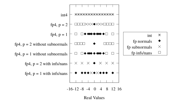
As highlighted by the normalization in Figure 1, it is often more natural to frame the quantization scheme in terms of a threshold $\gamma$ using the simple conversion $\gamma=\alpha\times\beta_{max}$, or more explicitly

$$\beta_{max}\leq\begin{dcases}2^{n-1}-1&\qquad\text{if }p=n-1\\ 2^{2^{n-p-1}-2}\times\left(2^{p+1}-1\right)&\qquad\text{if }p<n-1,\end{dcases}$$ (5)

where equality comes from using the full range by excluding Infs/NaNs. In other words, scale $\alpha$ represents the smallest positive subnormal value if subnormals were included, and threshold $\gamma$ represents the largest positive value allowed in the quantization scheme.

2.2 Operations

Basic arithmetic operations, that is binary operations between dynamic floating-point data types, are just simple cases of more advanced operations found in CNNs. In this section we define two advanced operations that in turn also define binary multiplication and addition.

If given dynamic floating-point numbers $x_{i}=\alpha_{x}\times\beta_{x_{i}}$ and $y_{i}=\alpha_{y}\times\beta_{y_{i}}$ such that $n_{x}=n_{x_{i}}$, $n_{y}=n_{y_{i}}$, $p_{x}=p_{x_{i}}$, and $p_{y}=p_{y_{i}}$ for all $i$, then the multiplication and accumulation found in convolution and inner product layers is expressed as follows:

$$z=\alpha_{z}\times\beta_{z}=\sum_{i=0}^{N-1}\left(x_{i}\times y_{i}\right)=\alpha_{z}\times\frac{\alpha_{x}\times\alpha_{y}}{\alpha_{z}}\times\sum_{i=0}^{N-1}\left(\beta_{x_{i}}\times\beta_{y_{i}}\right).$$ (6)

Now suppose that $\left[a_{x},b_{x}\right]$ and $\left[a_{y},b_{y}\right]$ are ranges with the smallest upper-bounds such that they contain every $\beta_{x_{i}}$ and $\beta_{y_{i}}$, respectively, where $b_{x}\geq 1$, $b_{y}\geq 1$, $a_{x}=-b_{x}-\epsilon_{x}$, $a_{y}=-b_{y}-\epsilon_{y}$, and $\epsilon_{x},\epsilon_{y}\in\mathbb{Z}_{\geq 0}$. Without loss of generality let $a_{y}\times b_{x}\leq a_{x}\times b_{y}$, and since by construction $a_{x}\times a_{y}\geq b_{x}\times b_{y}$, then

$$\sum_{i=0}^{N-1}\left(\beta_{x_{i}}\times\beta_{y_{i}}\right)\in\left[N\times a_{y}\times b_{x},N\times a_{x}\times a_{y}\right].$$ (7)

We can compute the sum of products above using a $q$-bit two’s complement signed-integer accumulator without loss of accuracy so long as $-2^{q-1}\leq N\times a_{y}\times b_{x}$ and $N\times a_{x}\times a_{y}\leq 2^{q-1}-1$. Therefore the smallest $q$ is

$$q=\left\lceil\log_{2}\left(N\times\left(b_{x}+\epsilon_{x}\right)\times\left(b_{y}+\epsilon_{x}\right)+1\right)+1\right\rceil$$ (8)

and the largest $N$ is

$$N=\left\lfloor\left(2^{q-1}-1\right)/\left(\left(b_{x}+\epsilon_{x}\right)\times\left(b_{y}+\epsilon_{y}\right)\right)\right\rfloor,$$ (9)

which generalizes a previous fixed-point analysis [7], and indicates that we should require $\epsilon_{x}=0$ and $\epsilon_{y}=0$ by always clamping IEEE floating-point values to $\left[-\gamma,\gamma\right]$ and reduced-precision floating-point values to $\left[-\beta_{max},\beta_{max}\right]$.

Next, if given dynamic floating-point numbers $x_{i}=\alpha_{x_{i}}\times\beta_{x_{i}}$ such that $n_{x}=n_{x_{i}}$ and $p_{x}=p_{x_{i}}$ for all $i$, then the addition found in eltwise addition layers is expressed as follows:

$$z=\alpha_{z}\times\beta_{z}=\sum_{i=0}^{N-1}x_{i}=\alpha_{z}\times\sum_{i=0}^{N-1}\left(\frac{\alpha_{x_{i}}}{\alpha_{z}}\times\beta_{x_{i}}\right).$$ (10)

Now suppose that $\left[a_{x},b_{x}\right]$ is a range with the smallest upper-bound such that it contains every $\beta_{x_{i}}$, where $b_{x}\geq 1$, $a_{x}=-b_{x}-\epsilon_{x}$, $\epsilon_{x}\in\mathbb{Z}_{\geq 0}$, and $\alpha_{x_{i}}\leq\alpha_{z}$, then

$$\sum_{i=0}^{N-1}x_{i}\in\left[N\times a_{x},N\times b_{x}\right].$$ (11)

We can compute the sum above using a $q$-bit two’s complement signed-integer accumulator without loss of accuracy so long as $-2^{q-1}\leq N\times a_{x}$ and $N\times b_{x}\leq 2^{q-1}-1$. Therefore the smallest $q$ is

$$q=\begin{dcases}\left\lceil\log_{2}\left(N\times b_{x}+1\right)+1\right\rceil&\qquad\text{if }\epsilon_{x}=0\\ \left\lceil\log_{2}\left(N\times b_{x}+N\times\epsilon_{x}\right)+1\right\rceil&\qquad\text{if }\epsilon_{x}\geq 1\end{dcases}$$ (12)

and the largest $N$ is

$$N=\begin{dcases}\left\lfloor\left(2^{q-1}-1\right)/b_{x}\right\rfloor&\qquad\text{if }\epsilon_{x}=0\\ \left\lfloor 2^{q-1}/\left(b_{x}+\epsilon_{x}\right)\right\rfloor&\qquad\text{if }\epsilon_{x}\geq 1,\end{dcases}$$ (13)

which further supports our decision to require $\epsilon_{x}=0$.

3 Quantization Procedure

An ideal quantization procedure for CNNs is one that with little effort can be made backwards compatible with existing hardware and software. Additionally, it is preferential to be able to reuse existing models to save the time of training from scratch, as featured in Ristretto [10, 11] and Google’s TensorFlow [17]. In fact, one would rather not retrain as even that can be time consuming or require the entire labeled data set which may not be available. Another method found in Google’s TensorFlow determines some 8-bit fixed-point quantization parameters online for each batch during inferencing [8], though it does have hooks to save and load these parameters offline. Elsewhere, NVIDIA’s TensorRT determines 8-bit fixed-point quantization parameters offline by inferencing with an unlabeled calibration set and at each layer analyzing the difference between the reference floating-point and fixed-point probability distribution functions [21]. Our method supports any dynamic floating-point scheme and a unified offline/online quantization flow with additional enhancements we found necessary for end-to-end post quantization accuracies. In order to limit the scope of this paper, we present our quantization procedure as it pertains to offline quantization.

In our method an IEEE 754 floating-point value in a tensor is converted to its reduced-precision floating-point value $\beta$ by first clamping the IEEE 754 floating-point value to a strictly symmetric threshold range $[-\gamma,\gamma]$. The threshold value $\gamma$ may be directly chosen from some statistical analysis of the aforementioned tensor such as a percentile or number of standard deviations, or from similar analyses of historically comparable tensors as shown in Algorithm 1 using a weighted average of over a dozen measures [4], though others have used just the Kullback-Leibler-I with reported success [21]. Next, the clamped value is divided by its scale $\alpha$, then the result proceeds through several more steps in order to round to the desired $\beta$. A reduced-precision floating-point value $\beta$ is converted to an IEEE 754 floating-point value by simply multiplying through by its scale $\alpha$.

Algorithm 1 Thresholding dynamic floating-point values

1:function threshold($x,n,p$)

2:     $pdf,bin\_edges\leftarrow hist(abs(x));cdf\leftarrow cumsum(pdf)$

3:     $\delta\leftarrow\infty;\gamma\leftarrow bin\_edges[-1]$

4:     for $i\leftarrow pow(2,n-1)+1,len(bin\_edges)-1$ do

5:         $r\leftarrow cdf;r[i-1:]\leftarrow 1$

6:         $r\_interp\leftarrow interp(fpspace(0.,1.,n,p),linspace(0.,1.,i),r[:i])$

7:         $q\_interp\leftarrow interp(linspace(0.,1.,i),fpspace(0.,1.,n,p),r\_interp)$

8:         $q\leftarrow r$; $q[:i]\leftarrow q\_interp$

9:         $\delta_{tmp}\leftarrow measure(cdf,q);\gamma_{tmp}\leftarrow bin\_edges[i])$

10:         if $\delta>\delta_{tmp}$ then

11:              $\delta\leftarrow\delta_{tmp};\gamma\leftarrow\gamma_{tmp}$

12:         end if

13:     end for

14:     return $\gamma,\delta$

15:end function

We begin our quantization procedure with a few preprocessing steps to prepare the network. Where possible we merge adjacent fork/join memory operations, e.g., multiple concat layers may be combined into a single concat layer. Likewise, any adjacent layers that are linear operations, e.g., batchnorm, scale, bias, convolution, and inner product layers, are combined into either a convolution or inner product layer. If an adjacent convolution or inner product layer does not exist, an identity convolution or inner product layer is created and inserted accordingly. Splicing in identity operations such as the aforementioned layers is a technique we heavily use to give us the ability to explicitly downscale reduced-precision floating-point values during end-to-end post quantization execution by factors we empirically find during the remainder of our quantization procedure to be on the interval $(0,1]$. Where these factors are determined to be unity, i.e., remain identity operations, then those layers are spliced back out. We apply this technique on edges directly connecting fork layers to join layers, and before join layers that directly, or indirectly, could not otherwise be explicitly downscaled, e.g., a maxpool layer following an eltwise layer.

Once the preprocessing steps are complete we iterate through the network quantizing weights with threshold values equal to the maximum absolute value per respective output channel. Meanwhile, threshold values for activations are measured in a bootstrap quantization fashion instead of a divide and conquer approach. Note that the choice of thresholds for biases may either be a function of input thresholds and weight thresholds or output thresholds depending on the target hardware implementation. Furthermore, the determination of threshold values for activations is delayed as long as possible so as to not prematurely drop least significant bits causing irreversible loss of information. For example, the threshold of a convolution layer–as specified by its associated scaling factor in Equation 6–followed by a ReLU layer is not determined until after the ReLU layer. In particular, this lazy thresholding is necessary to match the scaling factors associated with each input to joining layers such as concat and eltwise layers as indicated in Equation 10.

4 Experiments

We conducted three sets of dynamic floating-point quantization experiments that each target a variety of modern network features, mainly inception layers, residual layers, and grouped convolution layers in GoogLeNet v1 [23, 9], ResNet-50 [12, 13], and MobileNet v1 [15, 24], which we will henceforth simply refer to as GoogLeNet, ResNet, and MobileNet, respectively. Each of these models were trained by their authors on the ImageNet data set using single-precision floating-point. We chose GoogLeNet and ResNet as they represent networks typically deployed in data centers, and MobileNet because it is more indicative of networks designed for embedded devices. For each set of experiments we performed our quantization procedure for a calibration set chosen randomly without replacement from the training images and then measured the Top-1 inference accuracies for each set of experiments against 1600 validation images. Throughout the three sets of experiments we also varied the calibration set size between between 8, 32, and 128 to measure its relative effect on accuracies. Finally, unless otherwise mentioned, we include subnormals but exclude Infs/NaNs from our quantization scheme.

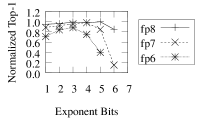
4.1 Subnormals and Infs/NaNs

The first set of experiments measure the effect of excluding subnormals or including Infs/NaNs since both reduce the numeric values representable by our quantization scheme, see Figures 2, 3, and 4. Here we use the same quantization scheme for weights as we do for activations. For the same bitwidth, Figure 3 shows no discernible difference in accuracies compared to Figure 2, while Figure 4 exhibits a significant drop in accuracies with fewer than 3 exponent bits. In fact, in each experiment there is no significant improvement in accuracies with more than 3 exponent bits. Finally, compared to results for a single exponent bit in Figure 2, which are by definition dynamic fixed-point schemes, there is between a 1–30% improvement in accuracies when using dynamic floating-point schemes of the same bitwidth and 3 exponent bits. This improvement is more pronounced in MobileNet, less so in ResNet, negligible in GoogLeNet, and generally more significant for smaller bitwidths.

(a) GoogLeNet

(b) ResNet

(c) MobileNet

Figure 2: With subnormals but without Infs/NaNs, calibrated against 128 training images

(a) GoogLeNet

(b) ResNet

(c) MobileNet

Figure 3: With subnormals and Infs/NaNs, calibrated against 8 training images

(a) GoogLeNet

(b) ResNet

(c) MobileNet

Figure 4: Without subnormals or Infs/NaNs, calibrated against 8 training images

4.2 Activations and Weights

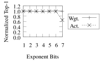
The second set of experiments measure the effect of trading exponent bits for significand bits on the activations and weights for $n=8$, see Figure 5. When testing the response for activations we set $p=4$ for the weights, and when testing the response for weights we set $p=4$ for the activations. From Figure 5 we see that activations and weights both need at least a few significand bits, but beyond that there is no significant difference in accuracies between activations and weights or more significand bits.

(a) GoogLeNet

(b) ResNet

(c) MobileNet

Figure 5: Activations and weights based on $n=8$, $p=4$, calibrated against 32 training images

4.3 Exponent and Significand Bits

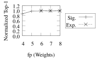
The third and final set of experiments measure the effect of reducing the bitwidth of the weights at the cost of either exponent bits or significand bits all while setting $n=8$ and $p=4$ for activations, see Figure 6. When testing the response on weights for exponent bits we start with $n=8$ and $p=4$ and decrement $n$ by one until $n=6$ all while keeping $p=4$. Similarly, when testing the response on weights for significands bits we start with $n=8$ and $p=4$ and decrement both $n$ and $p$ by one until $p=0$. In Figure 6 it appears that weights for GoogLeNet and ResNet can scale down from 8 bits to only 5 bits without significant loss in accuracies, but for MobileNet weights can only scale down to 7 bits before loss in accuracies become prohibitive. Furthermore, weights appear less sensitive to the exact allocation of exponent bits versus significand bits, but instead respond to the bitwidth itself.

(a) GoogLeNet

(b) ResNet

(c) MobileNet

Figure 6: Exponent and significand bits based on $n=8$, $p=4$, calibrated against 8 training images

5 Discussion

Our dynamic floating-point quantization scheme and procedure yields end-to-end post quantization inference accuracies similar if not indistinguishable to reference single-precision floating-point models by calibrating against a single inference batch, all while shrinking hardware and energy costs by 4x or more by replacing 32-bit operations with reduced-precision operations of 8-bits or fewer. In particular, we achieve 100% normalized top-1 accuracies for GoogLeNet for fp8 through fp6, whereas Intel recently reported slightly exceeding 60% for fp8 [2]. Furthermore, we found that for fp8 the best accuracies were obtained using $p=4$ or $p=3$. Our method allows Xilinx FPGA users to create custom circuit designs for various $n,p$ quantization parameters and reconfigure their FPGAs to match each target network’s optimal parameters. In fact, our results show that one can achieve accurate inference results with as few as 3 exponent bits and that 4 exponent bits is generally no better than 3 exponent bits, which would seem to contradict a prevailing belief popularized by NVIDIA that "fp16 is great, what’s actually even better than fp16 is truncated fp32" [5]. Nevertheless, cost savings are even available for a variety of existing hardware by increasing the effective bandwidth, reducing the effective on- and off-chip storage, even reducing the effective toggle rate by using $p=6$, a.k.a. int8, or $p=2$, a.k.a. truncated half-precision floating-point that can be casted on-the-fly to and from full half-precision floating-point to perform arithmetic operations, albeit both at the potential cost of inference accuracies. We also demonstrated that for some networks fp7 and fp6 are viable alternatives to fp8 with $p=3$ and achieved inference accuracies superior to their dynamic fixed-point scheme analogues, which can only be explained by the greater range and increased precision about zero provided by our dynamic floating-point scheme. Thus for the densest compute platform developers may reconfigure a Xilinx FPGA for a particular $n,p$ configuration that meets their inference accuracy requirements. Since we’re not (re)training here, our dynamic floating-point quantization scheme and procedure can be thought of as an offline network compression with as few as eight calibration images, which could even potentially be substituted with artificial images obtained by playing the network in reverse. Finally, we’re confident that we could scale down even further if allowed to re(train) with quantization-in-the-loop (QIL) like [11] given that our accuracies are just as good or better using only a small calibration set.

References

- [1] IEEE standard for floating-point arithmetic. IEEE Std 754-2008, pages 1–70, 2008.
- [2] G. R. Chui, A. C. Ling, D. Capalija, A. Bitar, and M. S. Abdelfattah. Flexibility: FPGAs and CAD in deep learning acceleration. ISPD, 2018.
- [3] M. Courbariaux, Y. Bengio, and J.-P. David. Training deep neural networks with low precision multiplications. arXiv:1412.7024, 2014.
- [4] P. D’Alberto and A. Dasdan. Non-Parametric Information-Theoretic Measures of One-Dimensional Distribution Functions from Continuous Time Series, pages 685–696. 2009.
- [5] B. Dally. Scaling of machine learning. Scaled ML, https://www.youtube.com/watch?v=h3QKvUPg_AI, 2018.
- [6] W. Dally. High-performance hardware for machine learning. NIPS Tutorial, 2015.
- [7] Y. Fu, E. Wu, and A. Sirasao. 8-bit dot-product acceleration. White Paper: UltraScale and UltraScale+ FPGAs, 2017.
- [8] Google. TensorFlow. https://github.com/tensorflow/tensorflow/tree/r1.5/tensorflow/tools/graph_transforms, 2017.
- [9] S. Guadarrama. BVLC GoogLeNet. https://github.com/BVLC/caffe/tree/master/models/bvlc_googlenet, 2014.
- [10] P. Gysel, M. Motamedi, and S. Ghiasi. Hardware-oriented approximation of convolutional neural networks. arXiv preprint arXiv:1604.03168, 2016.
- [11] P. Gysel, J. Pimentel, M. Motamedi, and S. Ghiasi. Ristretto: A framework for empirical study of resource-efficient inference in convolutional neural networks. IEEE Transactions on Neural Networks and Learning Systems, pages 1–6, 2018.
- [12] K. He, X. Zhang, S. Ren, and J. Sun. Deep risidual learning for image recognition. arXiv:1512.03385, 2015.
- [13] K. He, X. Zhang, S. Ren, and J. Sun. Deep residual networks. https://github.com/KaimingHe/deep-residual-networks, 2016.
- [14] M. Horowitz. 1.1 computing’s energy problem (and what we can do about it). In 2014 IEEE International Solid-State Circuits Conference Digest of Technical Papers (ISSCC), pages 10–14, 2014.
- [15] A. G. Howard, M. Zhu, B. Chen, D. Kalenichenko, W. Wang, T. Weyand, M. Andreetto, and H. Adam. MobileNets: Efficient convolutional neural networks for mobile vision applications. CoRR, abs/1704.04861, pages 1,2,7,8,12,13, 2017.
- [16] F. N. Iandola, M. W. Moskewicz, K. Ashraf, S. Han, W. J. Dally, and K. Keutzer. SqueezeNet: AlexNet-level accuracy with 50x fewer parameters and 1MB model size. arXiv:1602.07360, 2016.
- [17] B. Jacob, S. Kligys, B. Chen, M. Zhu, M. Tang, A. Howard, H. Adam, , and D. Kalenichenko. Quantization and training of neural networks for efficient integer- arithmetic-only inference. arXiv:1712.05877v1, 2017.
- [18] A. Krizhevsky. cuda-convnet. https://code.google.com/archive/p/cuda-convnet/, 2012.
- [19] A. Krizhevsky, I. Sutskever, and G. E. Hinton. Imagenet classification with deep convolutional neural networks. In Advances in Neural Information Processing Systems, pages 1097–1105, 2012.
- [20] Y. Lecun, L. Bottou, Y. Bengio, and P. Haffner. Gradient-based learning applied to document recognition. Proceedings of the IEEE, pages 2278–2324, 1998.
- [21] S. Migacz. 8-bit inference with TensorRT. GPU Technology Conference, 2017.
- [22] K. Simonyan and A. Zisserman. Very deep convolutional networks for large-scale image recognition. arXiv:1409.1556, 2014.
- [23] C. Szegedy, W. Liu, Y. Jia, P. Sermanet, S. Reed, D. Anguelov, D. Erhan, V. Vanhoucke, and A. Rabinovich. Going deeper with convolutions. arXiv:1409.4842, 2014.
- [24] S. Yang. MobileNet-Caffe. https://github.com/shicai/MobileNet-Caffe, 2017.