Fluctuation dissipation theorem and electrical noise revisited.

Abstract

The fluctuation dissipation theorem (FDT) is the basis for a microscopic description of the interaction between electromagnetic radiation and matter. By assuming the electromagnetic radiation in thermal equilibrium and the interaction in the linear response regime, the theorem interrelates the spontaneous fluctuations of microscopic variables with the kinetic coefficients that are responsible for energy dissipation. In the quantum form provided by Callen and Welton in their pioneer paper of 1951 for the case of conductors (H.B. Callen and T.A. Welton, Phys. Rev. 83 (1951) 34-40), electrical noise detected at the terminals of a conductor, is given in terms of the spectral density of voltage fluctuations, $S_{V}(\omega)$, was related to the real part of its impedance, $Re[Z(\omega)]$, by the simple relation:

$$S_{V}(\omega)=2\hbar\omega coth\left(\frac{\hbar\omega}{2K_{B}T}\right)Re\left[Z(\omega)\right]$$

where $K_{B}$ is the Boltzmann constant, $T$ is the absolute temperature, $\hbar$ is the reduced Planck constant and $\omega$ is the angular frequency. The drawbacks of this relation concern with: (i) the appearance of a zero point contribution which implies a divergence of the spectrum at increasing frequencies; (ii) the lack of detailing the appropriate equivalent-circuit of the impedance, (iii) the neglect of the Casimir effect associated with the quantum interaction between zero-point energy and boundaries of the considered physical system; (iv) the lack of identification of the microscopic noise sources beyond the temperature model. These drawbacks do not allow to validate the relation with experiments. By revisiting the FDT within a brief historical survey since the genesis of its formulation, that we fix with the announcement of Stefan-Boltzmann law (1879-1884), we shed new light on the existing drawbacks by providing further properties of the theorem with particular attention to problems related with the electrical noise of a two-terminals sample under equilibrium conditions. Accordingly, among the others, we will discuss the duality and reciprocity properties of the theorem, its applications to the ballistic transport regime, to the case of vacuum and to the case of a photon gas.

I Introduction

The fluctuation-dissipation theorem (FDT) is a pillar of statistical physics by interrelating the interaction between electromagnetic fields and matter. In essence, it asserts that linear response of a given system to an external perturbation is expressed in terms of fluctuation properties of the system in thermal equilibrium. Even if the FDT is generally associated with the announcement of Nyquist relation in 1928 nyquist28 , its genesis can be traced back to the Stefan-Boltzmann law of 1878-1884 that relates the total power radiated by a black-body to the fourth power of the absolute temperature. Since then, its formulation received particular attention by many scientists. Yet, to date several ambiguities and paradoxes remain which strongly hide the relevant power of this theorem in interpreting a large variety of physical phenomena. The aim of this paper is to revisit the FDT, and in particular its application to electrical noise, and shed new light on details and properties of the theorem that are usually not considered in the standard literature and/or are avoided because they inhibit to carry out a comparison between theory and experiments. While we attempt to describe a wide range of phenomena, this selection is by no means exhaustive, and highly biased by subjective interests. Significant examples are the individualization of the natural bandwidths of the fluctation spectra under classical conditions described by Nyquist relations, and the role of the zero-point contribution emerging under quantum conditions. Together with several original contributions, the review collects many results already available in the literature, with the purpose to provide a unifying picture for the benefit of a deeper understanding of the interaction between light and matter at a microscopic and macroscopic level. We believe that this paper, by touching the most relevant aspects of the subject within an historical survey, can also serve as a reference for a broad audience of scholars and researchers interested to further advance on the topic.

As physical system of interest we consider a cavity of length, $L$, and cross-sectional area, $A$, filled with a homogeneous medium with the terminal surfaces acting as ideal metallic contacts, and embedded in a thermal reservoir at a given temperature $T$. When the medium is replaced by vacuum the standard black-body is recovered. Here we mostly focus on: the instantaneous voltage fluctuations measured between the open terminals of the physical system and the real part of its impedance or the instantaneous current fluctuations measured in the short circuit connecting opposite terminals of the system and the real part of its admittance. The theoretical formulation of the FDT in the time domain implies an inter-relation between the correlation function, describing fluctuations of an observable (the noise), and the response function, describing the associated linear-response coefficient (the signal). By Fourier transform, these functions can be expressed in the frequency domain (spectra) thus allowing for an easier comparison of theory with experiments. Statistical mechanics under equilibrium conditions and linear-response theory to an external perturbation are the most rigorous way to provide a microscopic formulation of the FDT. We want to stress, that among the other, the above formulation of the FDT provides a unified interpretation of the black-body radiation spectrum and of the thermal agitation of electric charge in conductors.

From an historical point of view, the following steps provide a time sequence of the most important achievements that can be traced back to the FDT haar54 ; parisi01 ; boya04 .

1 - (1860), Kirchhoff kirchhoff1860 , On the relation between the radiating and absorbing powers of different bodies for light and heat.
2 - (1879-1884), Stefan-Boltzmann law for the total emissivity of a black-body at a given temperature.
3 - (1896-1905), Wien (1896), Rayleigh (1900), Planck (1901), Jeans (1905) laws for the power spectrum of the black-body radiation.
4 - (1905), Einstein einstein05 diffusion-mobility relation for a classical gas.
5 - (1908), Langevin langevin08 stochastic approach and fluctuation force.
6 - (1912), Planck planck12 inclusion of zero-point energy of a quantum oscillator.
7 - (1927), Johnson johnson27 thermal noise in conductors, experiments.
8 - (1928), Nyquist nyquist28 thermal noise in conductors, theory.
9 - (1931), Onsager onsager31 reciprocity relations of kinetic coefficients in irreversible processes.
10 - (1948), Casimir casimir48 attraction between opposite metallic plates in vacuum.
11 - (1951), Callen-Welton callen51 quantum fluctuation dissipation theorem for conductors.
12 - (1957), Kubo kubo66 quantum formalism of correlation and response functions.
Recent advances in the field comprise: FDT in the microcannical, canonical and grand-canonical ensembles, reciprocity and duality relations in the FDT, the role of Casimir effect in the black-body radiation spectrum bonanca08 ; reggiani16 ; reggiani17 .

According to the above historical survey, the first important manifestation of the FDT can be traced back from Stefan-Boltzmann black-body radiation law announced in the period 1879-1884, and relating light absorption and thermal radiation of a macroscopic body. The theoretical interpretation of the black-body radiation spectrum involved the formulation of the Rayleigh-Jean law of 1900 and then of the celebrated Planck law of 1901.

A second manifestation of the FDT was Einstein relation between mobility and diffusivity of 1905, that is at the basis of Brownian chaotic molecular-motion. The theoretical interpretation of the Brownian motion led Langevin to develop in 1908 a new theoretical approach based on stochastic differential equations.

A third manifestation of the FDT was the discovery by Johnson of the spontaneous electrical fluctuations between the terminals of a conductor at equilibrium in 1927 and the subsequent theoretical formulation by Nyquist in 1928.

A fourth manifestation of the FDT was the prediction by Casimir in 1948 of the existence of an attractive force between two parallel metallic plates in vacuum, which was associated with the unavoidable presence of the zero-point fluctuations of the electromagnetic field. This quantum agitation is due to the uncertainty principle and represents the vacuum counterpart of thermal agitation. Casimir prediction was later confirmed experimentally with increasing accuracy and theoretically justifiable within the quantum expression of the FDT formulated by Callen and Welton in 1951.

Theoretical modeling of FDT can be traced back to the Rayleigh-Jeans law, followed by Wien and Planck laws for the interpretation of black-body radiation spectrum. Then, further developments include Einstein relation and the Langevin formalism of stochastic differential equations, Nyquist relation for the interpretation of Johnson electrical noise, Callen and Welton quantum generalization of Nyquist relation, Kubo formalism and the use of a generalized quantum Langevin equation ford88 .

The most rigorous theoretical derivation of the FDT makes use of quantum statistical mechanics. To this purpose, fundamental advances started from Callen and Welton pioneer paper of 1951, where a first order perturbation theory was used, and Kubo operatorial formalism of 1957. In both cases use was made of a canonical ensemble approach. Bonanca 2008 bonanca08 derived the FDT for the case of a microcanonical ensemble and Reggiani et al reggiani16 for the case of a grand canonical ensemble, generalizing the results to the case of quantum fractional-statistics.

II Critical formulation of the fluctuation dissipation theorem

The essence of the problem addressed in this section can be formulated by considering the thermal noise-power per unit bandwidth, $dP(f)/df=u(f,T)$, with $u(f,T)$ the energy spectrum at frequency $f$ and temperature $T$ radiated into a single mode of the electromagnetic field by a physical system coupled to a thermal reservoir. As physical systems, here we consider the relevant cases of: (i) a one-dimensional harmonic oscillator and the fluctuations of the carrier displacement $X(t)$, (ii) a conductor and the fluctuations of the voltage drop at the open terminals $V(t)$, (iii) a conductor and the fluctuations of the current flowing in the short circuit $I(t)$. We notice that for an ideal black-body cavity the impedance coincides with the vacuum resistance given by $R_{vac}=\mu_{0}c$, with $\mu_{0}$ the vacuum permeability and $c$ the light speed in vacuum. Thus, the black-body can be considered as a particular case of a resistor.

For all the cases of interest $u(f,T)$ is a universal function of frequency and temperature given by:

$$u(f,T)=S_{X}(f)\frac{2\pi f}{4Im\{\alpha_{x}(f)\}}\,$$ (1)

$$u(f,T)=S_{V}(f)\frac{1}{4Re\{Z(f)\}}\,$$ (2)

$$u(f,T)=S_{I}(f)\frac{1}{4Re\{Y(f)\}}\,$$ (3)

where $S(f)$ is the (symmetrized) spectral-density of the fluctuations of the corresponding observable $X,V,I$, and $\alpha_{x}(f)$ (the electrical susceptibility), $Z(f)$ (the impedance) and $Y(f)=1/Z(f)$ (the admittance) are the response coefficients of the considered physical system.

The spectral density and the associated response coefficient are the Fourier-Laplace transform of the corresponding (symmetrized) correlation-function and of the response function in the time domain. Thus, by interrelating the fluctuations with the dissipative part of the response, the above expressions for $u(f,T)$ represent the mathematical formulation of the fluctuation dissipation theorem. Both the correlation and the response functions can be expressed within a classical or a quantum formalism, as will be detailed in the following. According to the literature, the thermal noise-power per unit bandwidth takes three possible universal forms as:

$$u_{RJ,N}(f,T)=K_{B}T\ ,$$ (4)

$$u_{P}(f,T)=K_{B}T\frac{x}{e^{x}-1}\ ,$$ (5)

$$u_{P,CW,K}(f,T)=K_{B}T\frac{x}{2}coth(\frac{x}{2})=u_{P}(f,T)+\frac{hf}{2}\ ,$$ (6)

where $u_{RJ,N}(f,T)$ refers to Rayleigh-Jeans and Nyquist nyquist28 classical formulation, $u_{P}(f,T)$ refers to Planck 1901 planck01 quantum formulation and $u_{P,CW,K}(f,T)$ refers to Planck 1912 planck12 , Callen-Welton 1951 callen51 and Kubo 1957 kubo66 quantum formulation including zero point contribution, with $x=hf/K_{B}T$ where $h$ is the Planck constant, and $K_{B}$ is the Boltzmann constant.

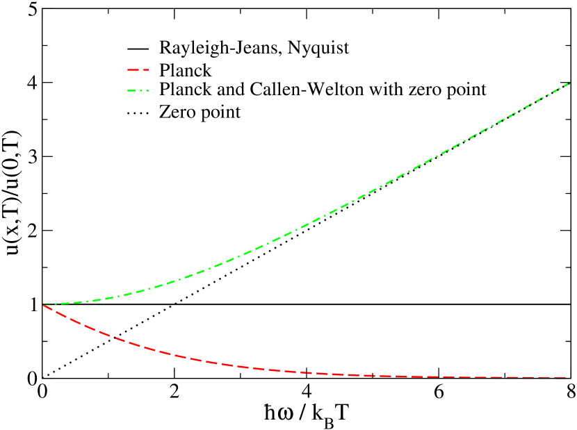
Figure 1: Different shapes of $u(x,T)$ with $x=\hbar\omega/(K_{B}T)$ according to different models: black continuous curve refers to Rayleigh-Jeans and Nyquist, red dashed curve refers to Planck black-body, green dot-dashed curve refers to Planck, Callen and Welton, Kubo with zero-point contribution included, black dotted curve refers to zero-point only.

We notice that Rayleigh-Jeans and Planck considered the black-body as the physical system of interest, while Nyquist, Callen and Welton, and Kubo considered basically a two terminal sample of given impedance (or admittance) without specifying the equivalent circuit, that is, the associated reactance. All the three forms satisfy the conditio:

$$u(f=0,T)=K_{B}T\,$$ (7)

a universal property valid for both classical and quantum physical systems.

The total energy, $U(T)$, associated with a black-body of volume $V_{0}$ is defined as:

$$U(T)=\sum u(f,T)=V_{0}\frac{8\pi}{c^{3}}\int_{0}^{\infty}f^{2}u(f,T)df\,$$ (8)

where the sum is extended over all the photon modes.

We stress that only the Planck form, $u_{P}(f,T)$ leads to a finite value of $U(T)$, in agreement with experiments and Stefan-Boltzmann law. By contrast, both the other two forms lead to a so-called ultra-violet catastrophe. We remark, that the split into two contributions of $u_{P,CW,K}(f,T)$, as given by the last expression in the r.h.s. of Eq. (5), is of most physical importance. Indeed, after integration over all frequency range each contribution leads to the macroscopic and exclusive value of the total-energy associated with the spectrum.

The first term is the Planck-contribution and represents a property of the coupling between the thermal reservoir and the physical system at thermal equilibrium. It follows from the detailed energy-balance related with the microscopic process of energy exchange between the thermal reservoir and the physical system. As such, it is a universal function of the temperature which takes a finite value at any frequency. Accordingly, it vanishes at $T=0$, it is independent of the external shape of the physical system and of the conducting material inside to the physical system. Its spectrum can be directly measured by standard experimental techniques in a wide range of frequencies, typically from mHz to THz, and excellent agreement between theory and experiments is a standard achievement. This contribution is the responsible of the thermal agitation at an atomic level of macroscopic bodies.

By contrast, the second term, $hf/2$, represents a quantum property of the vacuum, and from its definition, it does not vanish at $T=0$. Its expectation value diverges (a so called vacuum catastrophe) but it is responsible of an attractive or repulsive force acting between opposite surfaces of a confined physical-system, as predicted by Casimir in 1948 casimir48 for the simple case of two thin parallel conducting plates in vacuum. This Casimir force is now thought to pertain to a more general family of so called fluctuation-induced forces that are ubiquitous in nature, covering many topics from biophysics to cosmology kardar99 .

The essential difference between the above two contributions is better explained when considering the total energy obtained by summation over all the photon modes. For the Planck contribution, $U_{P}$, the summation is easily performed and gives the well-known result expressed by the Stefan-Boltzmann law for the total internal-energy associated with a black-body system at a given temperature:

$$U_{P}(T)=\sum K_{B}T\ \frac{x}{e^{x}-1}=\frac{2\pi^{5}V_{0}(K_{B}T)^{4}}{15c^{3}h^{3}}=2.7N_{p}K_{B}T\,$$ (9)

where the sum is extended over all the photon modes, and $N_{p}=2.02\times 10^{7}\ V_{0}T^{3}$ is the expected number of photons inside the volume $V_{0}$ of the physical system at the given temperature. We remark, that Eq. (9) expresses the Stefan-Boltzmann law in terms of thermal averages of the number of photons (modes) times the average photon energy in analogy with the case of a classical gas. Here the difference is that the instantaneous number of photons is not conserved and their average number is a function of temperature. Furthermore, being Bosons, photons interact in terms of the symmetric properties of their wave-functions. Accordingly, their bunching property is reflected in the coefficient $2.7$ slightly lower than the value of $3$ associated with the relativistic classical-massive case.

For the zero-point term, the same summation gives the expectation value of the zero-point total energy, $U_{zp}$, defined as

$$U_{zp}=\frac{1}{2}\sum hf.$$ (10)

The sum gives a puzzling divergent energy contribution callen51 ; Dirac34 when evaluated all over the space. Otherwise, as observed by Casimir casimir48 , real measurements are performed on finite-size systems where manifestations of zero-point energy are directly observable milton . In particular, the different content of electromagnetic energy inside and outside an assigned region produces a force that, in the case of two thin parallel conducting plates in vacuum, is attractive casimir48 . In general, Eq. (10) is solved by using specific boundary conditions related to: (i) the shape of the physical system, (ii) the material inside the physical system. Calculations are not easy to be performed ederly06 ; schmidt08 ; auletta09 , and here we report the simple but significant case considered by Casimir casimir48 and further confirmed by more detailed mathematical approaches milton :

$$U_{C}=-\frac{\pi Ahc}{1440L^{3}}.$$ (11)

The negative value of the Casimir energy, $U_{C}$, corresponds to an attractive force (the Casimir force) between opposite conducting plates, $F_{C}$, given by

$$F_{C}=-\frac{\pi hcA}{480L^{4}}.$$ (12)

As a consequence of this force, the physical system is not mechanically stable and the two opposite conducting plates forming the terminals would tend to implode lebowitz69 when left free to move. Following standard mechanical arguments, to keep the stability a reaction vincular-force $F_{RV}=-F_{C}$, mostly ascribable to the rigidity of the physical system associated with its elastic properties kittel04 , should be introduced. We remark, that for macroscopic physical systems of centimeter length-scale as considered here, both forces take negligible values (of the order of $10^{-23}\ N$). Accordingly, by accounting for the Casimir force and the associated vincular reaction, the resultant force is null, thus supporting the conjecture that at thermal equilibrium once mechanical stability is established zero-point energy cannot be extracted but its macroscopic effects are simply stored in the rigidity of the physical system.

Indeed, the omission of the whole zero-point energy in considering black-body radiation spectrum is often encouraged for all practical calculations kogan96 ; prigogine14 . This omission can be justified by the fact that quantum agitation of vacuum does not interfere with particle thermal-agitation in a medium, rather it can be exactly compensated by forcing the stability of the physical system. We shall therefore drop the zero-point contribution in the expression (6) for the energy spectrum and recover the celebrated Planck distribution. As a consequence, the original Planck 1901 planck01 expression for the black-body radiation emission as well as the Nyquist relation for the electrical noise in dissipative conductors which replaces $K_{B}T$ by the Planck distribution (as originally suggested by Nyquist himself nyquist28 ) are justified, in full agreement with experimental evidence.

III Derivation of fluctuation dissipation theorem within a microcanonical ensemble

Following bonanca08 , this scheme assumes an isolated system whose dynamics is given by the Hamiltonian $H$. An external harmonic perturbation of the form, $\hat{V}=-xf(t)$, is then applied to the system, where $f(t)$ is a classical force depending on time and $x$ is the displacement operator.

By taking the expression for the microcanonical density operator, $\rho_{m}$, as:

$$\rho_{m}(E_{t})=\frac{E_{t}-H}{Z(E_{t})}$$ (13)

where $Z(E_{t})=Tr\delta(E_{t}-H)$, with $E_{t}$ the total energy of the system, to derive the FDT use is made of the representation of $\delta(E_{t}-H)$ as inverse Laplace transform:

$$\delta(E_{t}-H)=\frac{1}{2\pi i}\int_{\gamma-i\infty}^{\gamma+i\infty}exp[(E_{t}-H)z]dz$$ (14)

from which the quantum correlation function is introduced

$$C_{xx}(z,t)=Tr(e^{-Hz}x(0)x(t))$$ (15)

and the corresponding asymmetric spectral density

$$J_{xx}(\omega)=\frac{1}{2\pi}\int_{-\infty}^{\infty}C_{xx}(z,t)e^{-i\omega t}dt$$ (16)

satisfying the condition of detailed-energy balance:

$$J_{xx}(z,-\omega)=exp(-\hbar\omega z)J_{xx}(z,\omega).$$ (17)

By considering the macroscopic displacement due to the action of an harmonic potential, the symmetrized spectral-density of spontaneous fluctuations, $S_{xx}(z,\omega)$, and the Fourier transform of the linear-response-function measured through the same observable $x$, $\chi_{xx}(z,\omega)$, are given by

$$\biggl{[}{{S_{xx}(z,\omega)}\atop{\frac{1}{i\hbar}\{\chi_{xx}(z,\omega)\}}}\biggr{]}={1\over 2}\biggl{[}{{J_{xx}(z,\omega)+J_{xx}(z,-\omega)}\atop{J_{xx}(z,\omega)-J_{xx}(z,-\omega)}}\biggr{]}$$ (18)

From the above set of equations we obtain

$$S_{xx}(z,\omega)={\frac{i\hbar}{2}}coth(\frac{z\hbar\omega}{2})\ \chi_{xx}(z,\omega)\$$ (19)

which is the quantum FDT relating the spectra of the correlation function (i.e. fluctuations) and of the response function (i.e. dissipation).

In the classical limit $\hbar\rightarrow 0$ it is

$$S_{xx}(z,\omega)=\frac{i}{z\omega}\ \chi_{xx}(z,\omega)\$$ (20)

which is the classical FDT.

One easily realizes from Eqs. (19) and (20) that the replacement of $z$ by $1/(K_{B}T)$ in those equations leads precisely to the quantum and classical versions of the FDT obtained in the canonical ensemble zubarev71 ; landau74 .

We remark that Eq. (19), by containing the zero-point contribution, predicts the vacuum catastrophe already discussed in Sect (II). As a consequence, Eq. (19) is not appropriate to be compared with experiments. Rather, fluctuations in this case happen due to the dynamics of the concerned system itself and not due to the coupling to a thermostat as in the canonical ensemble. In addition to the pure meaning of the relation between response and correlation, one may wonder whether Eqs. (19) and (20) can be useful or not. Although beyond the scope of the present work, a general and deep discussion of the subtle points mentioned above as well as of the linear response theory for the microcanonical ensemble, would remain of great interest and value.

IV Classical Langevin approach

Here we express the spectral density and the kinetic coefficients entering the definition of $u(f,T)$ within a classical stochastic approach introduced by Langevin langevin08 . To justify a one dimensional treatment and neglect magnetic effects we consider the condition $L^{2}\ll A$, where an instantaneous number of carriers $N(t)$ are present in the physical system. From total-current conservation and Ramo-Shockley-Pellegrini theorem shockley38 ; ramo39 ; pellegrini86 ; pellegrini93 it is:

$$\frac{d}{dt}V(t)=\frac{L}{\varepsilon_{0}\varepsilon_{r}A}\left[\frac{q}{L}\sum_{i=1}^{N(t)}v_{i,x}(t)+I(t)\right]$$ (21)

with $V(t)$ the instantaneous voltage drop at the sample terminals, $\epsilon_{0}$ and $\epsilon_{r}$ the vacuum permittivity and the relative dielectric constant of the medium, respectively, $q$ the unit charge, $v_{i,x}(t)$ the instantaneous longitudinal velocity of the $i$-th carrier inside the sample, and $I(t)$ the instantaneous total-current.

Then, a Drude-Langevin equation is added to describe the electron motions inside the system:

$$m\frac{d}{dt}v_{d}(t)+\frac{m}{\tau}v_{d}(t)=-\frac{q}{L}V(t)+\Gamma(t)$$ (22)

where $v_{d}(t)$ is the instantaneous drift-velocity of carriers inside the sample, $m$ is a carrier effective mass, $\tau$ is the momentum scattering-time, and $\Gamma(t)$ is the instantaneous Langevin random-force satisfying,

$$\overline{\Gamma(t)} = 0$$ (23)

$$\overline{\Gamma(t)\Gamma(t^{\prime})} = \gamma\delta(t-t^{\prime})$$ (24)

where $\gamma$ is the strength of the noise source and overline denotes ensemble average.

By using the plasma frequency $\omega_{p}$

$$\omega_{p}^{2}=\frac{\overline{N}q^{2}}{\varepsilon_{0}\varepsilon_{r}mAL}$$ (25)

and the definition of the carrier drift-velocity

$$v_{d}(t)=\frac{1}{N(t)}\sum_{i=1}^{N(t)}v_{i,x}(t)$$ (26)

where $v_{i,x}(t)$ is the instantaneous value of the $i$-th carrier velocity component along the $x$ direction, we obtain

$$\frac{d}{dt}V(t)=\frac{mL}{\overline{N}}\omega_{p}^{2}\left[\frac{q}{L}N(t)v_{d}(t)+I(t)\right]$$ (27)

Now, the lumped equivalent-circuit and the two extreme boundary conditions associated with the detection of the electrical fluctuations are considered.

IV.1 Equivalent circuit and spectral densities

The equivalent circuit of a real resistor (conductor) which is consistent with the Langevin approach is shown in Fig. (2).

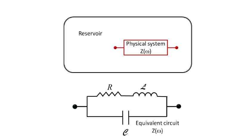
Figure 2: Schematic of the statistical ensemble considered here. The reservoir can be a grand-canonical or a canonical according to the operation conditions for noise detection at constant current or constant voltage operation modes, respectively. The equivalent circuit of the intrinsic impedance $Z(\omega)$ consists of a resistor $R$ with length L and cross sectional are A, a kinetic-inductance ${\cal L}$ and a parallel plates capacitor $\cal{C}$ filled with the homogenous medium that constitutes the resistor of given relative dielectric-constant. The capacitance and inductance account for the presence of the contacts and for the inertia of carriers, respectively. See text for details.

Here the Ohmic resistance independent of frequency is coupled with the intrinsic capacitance $\cal{C}$, that accounts for contact effects, and the intrinsic kinetic-inductance ${\cal L}$, that accounts for inertial effects of charge carriers. Accordingly, the impedance (admittance) $Z(\omega)$ ($Y(\omega)$) of the equivalent circuit is given by

$$Z(\omega)=\frac{1}{Y(\omega)}=R\frac{1+i\omega\tau}{1-\omega^{2}\tau_{p}^{2}+i\omega\tau_{d}}$$ (28)

$$Re[Z(\omega)]=R\frac{1}{(1-\omega^{2}\tau_{p}^{2})^{2}+\omega^{2}\tau_{d}^{2}}$$ (29)

$$Re[Y(\omega)]=G\frac{1}{1+\omega^{2}\tau^{2}}$$ (30)

where: the resistance is given by

$$R=\frac{1}{G}=\frac{L^{2}m}{q^{2}\overline{N}\tau}$$ (31)

with $G$ the conductance. The kinetic inductance is given by

$${\cal L}=\frac{A}{L}\mu_{0}\mu_{k}=\frac{L^{2}m}{q^{2}\overline{N}}$$ (32)

with $\mu_{k}$ the relative kinetic-permeability, and the capacitance is given by

$${\cal C}=\frac{A}{L}\epsilon_{0}\epsilon_{r}$$ (33)

As usual, the dielectric relaxation-time $\tau_{d}$, the scattering time $\tau$ and the plasma time $\tau_{p}$ are respectively given by:

$$\tau_{d}={\cal C}R,\ \tau={\cal L}/R,\ \tau_{p}^{2}={\cal CL}\,$$ (34)

Notice that for centimetric length-scale of the physical system and for a standard carrier density of $10^{22}\ cm^{-3}$ for a conductor material, the order of magnitude of $\cal C$ and $\cal L$ are respectively of $10^{-13}\ F$ and $10^{-19}\ H$. Therefore, in experiments parasitic capacitance and inductance should play a significant role, unless high resistivity materials are considered.

We remark that $Re[Y(\omega)]$ decays as a Lorentzian with the characteristic momentum relaxation-time. By contrast, $Re[Z(\omega)]$ decays with a spike at the plasma frequency, usually determining a plasmonic noise reggiani13 , which is washed out if the condition $\tau_{d}>\tau_{p}$ is satisfied. These spectra were validated by Monte Carlo simulations reggiani13 , even if, because of the ultra-high frequencies involved (typically over the THz range) a direct experimental confirmation is still lacking.

The above equivalent circuit is consistent with the standard energy-equipartition relations

$${\overline{V^{2}}}{{\cal C}}={\overline{I^{2}}}{{\cal L}}=K_{B}T,$$ (35)

which in this form are valid for any type of capacitance and inductance in the circuit reported by Fig. (2). As such, this equivalent circuit is of most physical importance and should replace alternative equivalent circuits (like, e.g., simple $R\cal C$ parallel and $R{\cal LC}$ series circuits) which are also sometimes used in the literature but that do not provide plausible physical-spectra.

IV.2 Current noise operation

In the current operation mode it is $V(t)=0$, carriers enter and exit from the contacts and the current noise is detected in the external short-circuit. The physical system should be considered an open one and is statistically described within a grand-canonical ensemble (GCE). Accordingly, the total current reads

$$I(t)=-\frac{q}{L}N(t)v_{d}(t)$$ (36)

and the Drude-Langevin equation writes

$$\frac{d}{dt}I(t)+\frac{1}{\tau}I(t)=\frac{\overline{N}q}{Lm}\Gamma(t)$$ (37)

In full agreement with the equivalent circuit shown in Fig. (2), the Drude-Langevin equation can also be written as

$$\frac{d}{dt}I(t)+\frac{R}{\cal L}I(t)=\frac{L}{q\cal L}\Gamma(t)$$ (38)

By using standard techniques mcquarrie , from the homogeneous equation the current correlation-function writes

$$C_{I}(t)=\overline{I(0)I(t)}=\overline{I^{2}}e^{-t/\tau}$$ (39)

and, from the inhomogeneous equation and energy equipartition, it is

$$\overline{I^{2}}=\frac{\overline{N}^{2}q^{2}}{2m^{2}L^{2}}\gamma\tau=\frac{K_{B}T}{\cal L}$$ (40)

Accordingly, the FDT relates $\gamma$ and $\tau$ as

$$\gamma\tau=\frac{2mK_{B}T}{\overline{N}}$$ (41)

From statistics, in the GCE the longitudinal diffusion-coefficient, generalized to include the effective interaction among carriers due to the symmetry properties of their wave functions and thus for the correct statistics gurevich79 , is given by

$$D=\overline{v^{2^{\prime}}_{x}}\tau=\frac{K_{B}T\tau}{m}\frac{\overline{N}}{\overline{\delta N^{2}}}$$ (42)

where $\overline{v^{2^{\prime}}_{x}}$ is the differential (with respect to carrier number) quadratic velocity component along the $x$-direction given by

$$\overline{v^{2^{\prime}}_{x}}=\sum_{\bf{k}}v^{2}_{x}\,\frac{\partial f(\varepsilon_{\bf{k}})}{\partial\mu_{0}}\frac{\partial\mu_{0}}{\partial\overline{N}}=\frac{K_{B}T}{m}\frac{\overline{N}}{\overline{\delta N^{2}}}\ .$$ (43)

with $\mu_{0}$ the chemical potential.

The main conclusion is that current fluctuations are associated with fluctuations of the total number of carriers inside the system that satisfy the Langevin equation:

$$\frac{d}{dt}\delta N(t)+\frac{1}{\tau}\delta N(t)=\frac{L}{\sqrt{\overline{v^{2^{\prime}}_{x}}}}\Gamma(t),$$ (44)

with the corresponding correlation function

$$C_{\delta N}(t)=\overline{\delta N(0)\delta N(t)}=\overline{\delta N^{2}}e^{-t/\tau}$$ (45)

and from statistics in the GCE it is

$$\overline{\delta N^{2}}=K_{B}T\frac{\partial\overline{N}}{\partial\mu_{0}}$$ (46)

From Wiener-Khinchin theorem, the current spectral-density reads

$$S_{I}(\omega)=\frac{4\overline{I^{2}}}{{\Delta f_{I}}}\ \frac{1}{1+(\omega\tau)^{2}}=4K_{B}TRe\{Y(\omega)\}$$ (47)

Equation (47) identifies $\Delta f_{I}=1/\tau$ as the natural bandwidth of the current fluctuations spectrum and together with Eqs. (40) and (42) recovers a microscopic definitions of conductance:

$$G=\left(\frac{q}{L}\right)^{2}D\frac{\partial\overline{N}}{\partial\mu_{0}}=\frac{q^{2}\overline{v^{2^{\prime}}_{x}}\tau}{L^{2}K_{B}T}\ \overline{\delta N^{2}}$$ (48)

which gives the generalized Einstein relation and expresses the conductance (i.e. dissipation) in terms of the variance of total carrier-number fluctuations (i.e. fluctuation), thus representing a microscopic form of the FDT within a GCE.

IV.3 Voltage noise operation

In the voltage operation mode it is $I(t)=0$, carriers remain inside to the physical system and the voltage noise is detected between the terminals of the external open circuit. The physical system should be considered a closed one and it is statistically described within a canonical ensemble CE, i.e. $\overline{N}=N=\textrm{constant}$. Accordingly, conservation of total current becomes

$$\frac{d}{dt}V(t)=\frac{mL}{q}\omega_{p}^{2}v_{d}(t)$$ (49)

and the Drude-Langevin equation reads

$$\frac{d^{2}}{dt^{2}}V(t)+\frac{1}{\tau}\frac{d}{dt}V(t)+\omega_{p}^{2}V(t)=\frac{L}{q}\omega_{p}^{2}\Gamma(t)$$ (50)

In full agreement with the equivalent circuit shown in Fig. 2, the Drude-Langevin equation can also be written as

$$\frac{d^{2}}{dt^{2}}V(t)+\frac{R}{\cal L}\frac{d}{dt}V(t)+\frac{1}{{\cal LC}}V(t)=\frac{L}{q{\cal LC}}\Gamma(t)$$ (51)

By using standard techniques mcquarrie , from the homogenous equation we obtain the correlation function

$$C_{V}(t)=\overline{V(0)V(t)}$$

$$=\overline{V^{2}}\left[\frac{e^{-\lambda_{1}t}\ \lambda_{2}}{\lambda_{2}-\lambda_{1}}+\frac{e^{-\lambda_{2}t}\ \lambda_{1}}{\lambda_{1}-\lambda_{2}}\right]$$ (52)

with

$$\lambda_{1,2}=\frac{1}{2\tau}\pm\sqrt{\frac{1}{4\tau^{2}}-\omega_{p}^{2}}$$ (53)

For $2\omega_{p}\tau<1$ the two real values of $\lambda$ describe a dumped behavior of $C_{V}(t)$, for $2\omega_{p}\tau>1$ the two complex conjugate values of $\lambda$ describe an oscillating behavior of $C_{V}(t)$.

From the inhomogeneous equation and energy equipartition, it is

$$\overline{V^{2}}=\frac{L^{2}\omega_{p}^{2}}{2q^{2}}\gamma\tau=\frac{K_{B}T}{\cal C}$$ (54)

Accordingly, the fluctuation-dissipation theorem relates $\gamma$ and $\tau$ as

$$\gamma\tau=\frac{2mK_{B}T}{\overline{N}}$$ (55)

From statistics, in the CE it is

$$\overline{\delta v_{d}^{2}}=\frac{1}{N^{2}}\sum_{\bf{k}}v_{x}^{2}\ \overline{\delta f^{2}(\varepsilon_{\bf{k}})}=\frac{K_{B}T}{m\ N}\ ,$$ (56)

where $\overline{\delta v_{d}^{2}}$ is the variance of the fluctuations of the instantaneous carrier drift-velocity inside the system, $v_{x}=\hbar k_{x}/m$ is the $x$-component of its velocity, $\bf{k}$ is the carrier wave vector, $\varepsilon_{\bf{k}}$ the corresponding energy and $\overline{\delta f^{2}}$ is the variance of the equilibrium distribution-function $f$ normalized to carrier number which, according to statistics, satisfies the property

$$\overline{\delta f^{2}(\varepsilon_{\bf{k}})}=-K_{B}T\frac{\partial f(\varepsilon_{\bf{k}})}{\partial\varepsilon_{\bf{k}}}\ ,$$ (57)

and, using the symmetry of the problem, $v_{x}^{2}$ is replaced by $(2\varepsilon_{\bf{k}}/md)$, where $d$ denotes the dimension of the system. With the density-of-states of a $d$-dimensional carrier gas satisfying ${\cal D}(\varepsilon)\propto\varepsilon^{(d/2)-1}$, Eq. (56) is independent of dimensionality.

Accordingly, we find

$$\overline{V^{2}}=\left(\frac{Lm\omega_{p}}{q}\right)^{2}\ \overline{\delta v_{d}^{2}}$$ (58)

From the equivalent circuit of Fig. (2), the spectral density reads

$$S_{V}(\omega)=\frac{4\overline{V^{2}}}{\Delta f_{V}}\ \frac{1}{(1-\omega^{2}\tau_{p})^{2}+(\omega\tau_{d})^{2}}$$

$$=4K_{B}TRe\{Z(\omega)\}$$ (59)

Equation (59) interpolates between the oscillating and damped behaviors of the correlation function of voltage fluctuations and identifies $\Delta f_{V}=1/\tau_{d}$ as the natural bandwidth of the voltage fluctuations spectrum. From Eqs. (56) and (58) the following microscopic definition of resistance is obtained:

$$R=\frac{L^{2}m^{2}}{q^{2}\tau K_{B}T}\overline{\delta v_{d}^{2}}.$$ (60)

which gives the resistance (i.e. dissipation) in terms of the variance of carrier drift-velocity fluctuations (i.e. fluctuation), thus representing a microscopic form of the FDT within a CE.

We conclude, that voltage fluctuations are associated with fluctuations of carrier drift-velocity inside the system.

IV.4 Damped harmonic oscillator

The Langevin equation for the damped harmonic oscillator is analogous to that of voltage fluctuations where voltage is substituted by carrier displacement along $x$ direction, i.e. $V(t)\rightarrow x(t)$, and the plasma frequency by the natural oscillator frequency, i.e. $\omega_{p}\rightarrow\omega_{0}$. The analogy is completed by noticing that the equipartition law writes $k\overline{x^{2}}=K_{B}T$, $k$ being the strength of the oscillator (spring constant) and $\overline{x^{2}}$ being the average squared-displacement along $x$ direction. Accordingly, the Langevin equation for the damped harmonic oscillator with $\omega_{0}=\sqrt{k/m}$ writes:

$${d^{2}\over dt^{2}}x+\gamma{d\over dt}x+\omega_{0}^{2}x=\frac{1}{m}\Gamma(t)$$ (61)

The corresponding spectral density is

$$S_{xx}(\omega)=\frac{4K_{B}T}{\omega}Im\{\alpha_{x}(\omega)\}$$ (62)

with $\alpha_{x}(\omega)$ the electrical susceptibility

$$\alpha_{x}(\omega)=\frac{m}{\omega_{0}^{2}-\omega^{2}+i(\gamma\omega)}$$ (63)

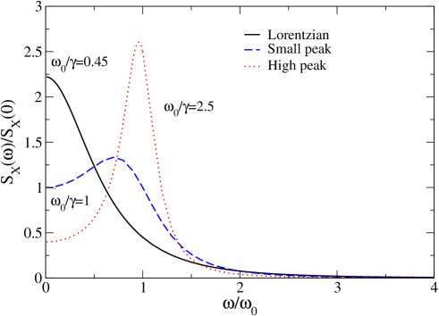
Figure 3: Shape of the normalized spectra of the damped harmonic oscillator for the cases: $\omega_{0}/\gamma=0.45$ continuous line, $\omega_{0}/\gamma=1$ dashed line, and $\omega_{0}/\gamma=2.5$ dotted line.

Figure (3) reports the shape of the spectra for the harmonic oscillator in the three cases: $\omega_{0}/\gamma=0.45$, $\omega_{0}/\gamma=1$, and $\omega_{0}/\gamma=2.5$. The spectra give evidence of the shift from a Lorentzian shape when $\omega_{0}<\gamma$ to a narrow peak centered at the natural oscillator-frequency when $\omega_{0}>\gamma$ as predicted by Eq. (62).

IV.5 Ballistic regime

The ballistic regime is controlled by the condition that the carrier transit time between opposite contacts, $\tau_{L}$, becomes shorter than the scattering time $\tau$. Then, by assuming for simplicity a one dimensional geometry, at equilibrium the single-carrier longitudinal velocity, $v_{x,b}$ inside the system remains constant in modulus.

In an open system, $v_{x,b}$ is controlled by the injection velocity-distribution. Following Landauer landauer99 , conductance becomes synonymous of transmission, i.e. all carriers that are injected at one contact are transmitted to the outside of the opposite contact. The value of the ballistic conductance, $G^{b}$, becomes independent of the length of the system and is given by

$$G^{b}=\frac{1}{R^{b}}=\frac{Aq^{2}n}{m\overline{v_{x,b}}}$$ (64)

with $R^{b}$ the ballistic resistance and $n$ the carrier concentration.

The ballistic resistance relies on a closed system where the ballistic carrier with a given $v_{x,b}$ is spectacularly reflected at the contacts. The transit time keeps the same value as for the case of conductance, but now resistance becomes synonymous of elastic reflection at the contacts and its value satisfies the reciprocity relation implied by Eq. (64).

For the case of a classical one-dimensional injection distribution, it is

$$\overline{v^{c}_{x,b}}=\sqrt{\frac{2\pi K_{B}T}{m}}=\frac{L}{\tau^{c}_{L}}$$ (65)

with $\tau^{c}_{L}=L/\overline{v^{c}_{x,b}}$ the transit time due to classical conditions, and for the equivalent circuit of Fig. 2 it is

$$\tau^{c}_{d}=R^{b,c}C=\frac{L^{2}}{{\lambda_{D}}^{2}}\tau^{c}_{L}$$ (66)

$$\tau^{c}=\frac{\cal L}{R^{b,c}}=\tau^{c}_{L}$$ (67)

$$\tau^{c}_{p}=\frac{L}{\lambda_{D}}\tau^{c}_{L}$$ (68)

with

$$\lambda_{D}=\sqrt{\frac{\epsilon_{0}\epsilon_{r}K_{B}T}{nq^{2}}}$$ (69)

the Debye length.

For the case of a degenerate one-dimensional injection distribution, it is greiner00

$$\overline{v^{d}_{x,b}}=v_{F}=\sqrt{\frac{2\epsilon_{F}}{m}}=\frac{L}{\tau^{d}_{L}}$$ (70)

with $v_{F}$ and $\epsilon_{F}=\hbar^{2}n_{1D}^{2}/(2m)$ the one dimensional Fermi velocity and Fermi energy, respectively, $n_{1D}$ the one dimensional carrier concentration, and $\tau^{d}_{L}=L/v_{F}$ the transit time associated with degenerate conditions.

For the equivalent circuit of Fig. 2 it is

$$R^{b,d}=\frac{1}{G^{b,d}}=\frac{h}{e^{2}}$$ (71)

per unit spin, and

$$\tau^{d}_{d}=R^{b,d}{\cal C}=\frac{L^{3}}{4\alpha cA}$$ (72)

$$\tau^{d}=\frac{{\cal L}}{R^{b,d}}=\frac{4\alpha L^{3}}{cA}$$ (73)

$$\tau^{d}_{p}=\frac{L^{6}}{c^{2}A^{2}}$$ (74)

with $\alpha=1/137$ the fine structure constant and $L^{3}/(cA)$ a geometrical-averaged relativistic transit-time associated with degenerate conditions.

We remark, that under ballistic conditions, since the absence of scattering makes the dynamics deterministic, the correlation functions of current fluctuations do not obey a simple exponential relaxation but a more complicated decay depending from the carrier statistics. According to greiner00 , the one-dimensional correlation functions of current fluctuations take the form, respectively for the ballistic-classical regime and the ballistic-degenerate regime:

$$\frac{C_{I}^{b,c}(x)}{C_{I}^{b,c}(0)}=erf(x^{-1})-x[1-exp(-x^{-2})],$$ (75)

and

$$\frac{C_{I}^{b,d}(x)}{C_{I}^{b,d}(0)} = 1-x\ for\ x\leq 1$$

$$= 0\ for\ x>1,$$

with $x$ the time normalized to the respective ballistic transit-time.

Figure (4) reports the one-dimensional correlation functions of current fluctuations given above.

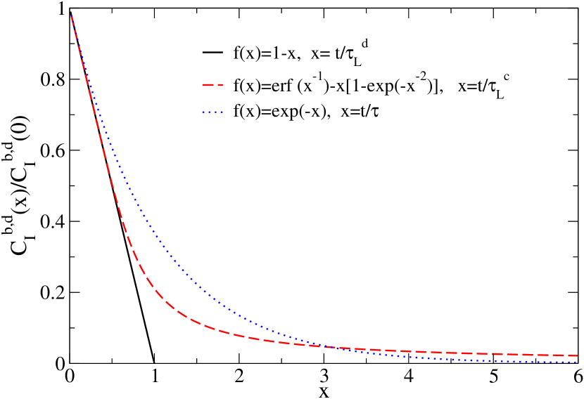
Figure 4: Shape of the correlation functions of current fluctuations normalized to its initial value at $t=0$ in the case of one-dimensional ballistic regime. Continuous curve refers to degenerate ballistic-conditions, dashed curve refers to classical ballistic-conditions, dotted curve refers to the case of an exponential decay typical of a diffusive regime.

Here curve 1 refers to the case of classical ballistic-conditions and the correlation function is found to exhibit a long-time limit decay as $t^{-3}$. Curve 2 refers to the case of degenerate ballistic-conditions, and the decay is found to exhibit a universal triangular shape. Curve 3 refers to the case of an exponential decay typical of a diffusive regime and is reported for the sake of comparison.

The longitudinal diffusion coefficient takes a form analogous to that of the diffusive regime, but with the differential quadratic-velocity replaced by the quadratic injection-velocity and the scattering time replaced by the ballistic transit-time. Thus, under ballistic conditions diffusion like conductance becomes a global quantity that depends on the sample length as

$$D^{c,d}_{b}=\overline{v^{c,d}_{x,b}}^{2}\tau^{c,d}_{L}=\overline{v^{c,d}_{x,b}}L$$ (77)

IV.6 Classical electrodynamics in vacuum

By considering the case of vacuum, for the classical electric-field averaged over the black-body length, $E=V/L$, the corresponding Langevin equation is obtained from that of voltage fluctuations and reads:

$$\frac{d^{2}}{dt^{2}}E(t)+\frac{1}{\tau_{E}}\frac{d}{dt}E(t)+\frac{1}{\tau_{E}^{2}}E(t)=\Gamma_{E}(t)$$ (78)

Using the vacuum definitions of resistance, capacitance and inductance there is a single time scale, $\tau_{E}=L/c$ and the correlation function takes the analytical form

$$C_{E}(t)=\overline{E(0)E(t)}$$

$$=\overline{E^{2}}e^{-t/2\tau_{E}}\times[asin(\frac{\sqrt{3}}{2}\frac{t}{\tau_{E}})+bcos(\frac{\sqrt{3}}{2}\frac{t}{\tau_{E}})]$$ (79)

with $a=1/4(\sqrt{3\pi/2}+\sqrt{\pi/6})=0.75$ and $b=\sqrt{\pi/2}=1.25$.

From classical energy-equipartition and FDT it is

$$\overline{E^{2}}=\frac{K_{B}T}{LA\epsilon_{0}}=\frac{K_{B}TR_{vac}}{A\tau_{E}}=\frac{\gamma_{E}\tau_{E}}{2}$$ (80)

For the classical magnetic-field averaged over the black-body geometry, $H=(L/A)I$ the corresponding Langevin equation is obtained from that of current fluctuations and reads:

$$\frac{d}{dt}H(t)+\frac{1}{\tau_{H}}H(t)=\Gamma_{H}(t)$$ (81)

with $\tau_{H}=\tau_{E}=L/c$ the correlation time of magnetic-field fluctuations.

The correlation function reads

$$C_{H}(t)=\overline{H(0)H(t)}=\overline{H^{2}}e^{-t/\tau_{H}}$$ (82)

From classical energy-equipartition and FDT it is

$$\overline{H^{2}}=\frac{K_{B}T}{LA\mu_{0}}=\frac{K_{B}TG_{vac}}{A\tau_{H}}=\frac{\gamma_{H}\tau_{H}}{2}$$ (83)

Figure (5) shows the correlation functions of the electric-field and magnetic-field fluctuations in vacuum given in Eqs. (79) and (82), respectively.

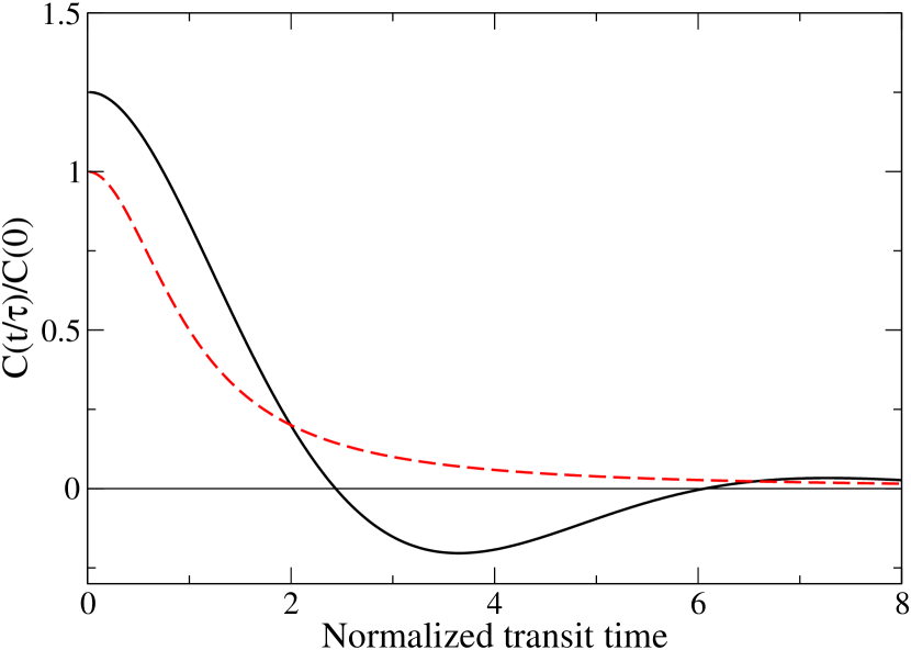
Figure 5: Correlation functions of the fluctuations of the classical electromagnetic fields in vacuum normalized to their initial value at $t=0$. Continuous curve refers to the electric field and dashed curve to the magnetic field, respectively.

For the spectral density of the electric-field fluctuations it is:

$$S_{E}(\omega)=\frac{4K_{B}TR_{vac}}{L^{2}}\frac{1}{1-(\omega\tau_{E})^{2}+(\omega\tau_{E})^{4}}$$ (84)

whose shape is the same of that of the damped harmonic oscillator reported in Fig. (3) when $\omega_{0}=1/\gamma=1/\tau_{E}$.

For the spectral density of the magnetic-field fluctuations it is:

$$S_{H}(\omega)=\frac{4K_{B}TG_{vac}L^{2}}{A^{2}}\frac{1}{1+(\omega\tau_{H})^{2}}$$ (85)

whose spectrum is a Lorentzian with $G_{vac}=1/R_{vac}$.

We notice that, under voltage operation mode, only the fluctuations of the electric field are detected, while for current operation mode only the fluctuations of the magnetic field are detected.

V Duality and reciprocity of fluctuation dissipation theorem

The dual property of electrical transport in the linear-response regime asserts that perturbation (applied voltage or imposed current) and response (measured current or voltage-drop) can be interchanged with the associated kinetic coefficients (resistance or conductance, respectively), being reciprocally interrelated. According to Ohm law, for a homogeneous conductor the dual property gives

$$V=RI\quad\mbox{and}\quad I=GV,$$ (86)

that implies the reciprocity relation

$$RG=1\ .$$ (87)

An analogous dual property and reciprocity relation can be formulated for electrical fluctuations at thermal equilibrium. Here the perturbation is the source of the microscopic fluctuations inside the physical system (carrier number or carrier drift-velocity), and the response is associated with the variance of the macroscopic fluctuating quantity (current or voltage). The individuation of the noise sources at a kinetic level, and thus beyond the simple thermal-agitation model, is a major issue in statistical physics that received only partial, and sometimes controversial, answers even in the basic literature johnson27 ; nyquist28 ; callen51 ; kubo66 ; klimontovich87 .

For the analysis at a kinetic level of current or voltage fluctuations a correct definition of the physical system becomes of primary importance. On the one hand, the microscopic interpretation of carrier transport implies the definition of an appropriate equivalent circuit at the macroscopic level. On the other hand, the detection of current or voltage fluctuations in the outside circuit should be related to the boundary conditions associated with the choice of the operation mode of detection (i.e. constant current or constant voltage) and the corresponding statistical ensemble of reference. Accordingly, current noise is measured in the outside short-circuit, which implies an open system that is permeable to carrier exchange with the thermal reservoir, thus referring to a grand canonical ensemble (GCE). By contrast, voltage noise is measured in the outside open-circuit which implies that carrier number in the system remains rigorously constant in time, thus referring to a canonical ensemble (CE). While it is well-known that in the thermodynamic limit different statistical ensembles become equivalent landsberg54 , this does not hold anymore in the case of fluctuations, where a finite-size system has to be considered. Nevertheless, we will show that the dual property provides a simple relation between the noise sources acting in the GCE and those acting in the CE. Typical examples of physical system of interest have been reported in the previous sections, where use was made of a standard Langevin approach. Here, the duality and reciprocity properties of the FDT are addressed and formally solved in the framework of the basic laws of statistical mechanics.

According to the reciprocity property of the linear-response coefficients and their definitions in terms of the microscopic noise sources given in Eqs. (48) and (60) it is:

$$GR=\frac{\overline{v^{2^{\prime}}_{x}}\overline{\delta N^{2}}m^{2}\overline{\delta v_{d}^{2}}}{(K_{B}T)^{2}}=\frac{\overline{v^{2^{\prime}}_{x}}}{\overline{\delta v_{d}^{2}}}\ \frac{\overline{\delta N^{2}}}{N^{2}}=1$$ (88)

Thus, the microscopic noise sources satisfy the duality relation

$$\overline{\delta N^{2}}\ \overline{v^{2^{\prime}}_{x}}={N}^{2}\ \overline{\delta v_{d}^{2}}\ =\frac{NK_{B}T}{m}.$$ (89)

For the variance of current fluctuations, substitution of Eq. (43) into Eq. (40) gives the equivalent expressions:

$$\overline{I^{2}}=\frac{q^{2}\delta\overline{N^{2}}}{\tau_{N}^{2}}=\frac{A^{2}}{L^{2}}\overline{H^{2}},$$ (90)

with $\tau_{N}=\sqrt{L^{2}/\overline{v^{2^{\prime}}_{x}}}$ an effective transport-time through the sample greiner00 determining the conversion of carriers total-number fluctuations inside the sample into total-current fluctuations measured in the external short-circuit, and with $\overline{H^{2}}$ the variance of magnetic-field fluctuations at equilibrium averaged over the geometry of the physical system. From Eq. (90), the expression

$$\overline{H^{2}}=\frac{L^{2}}{A^{2}}\overline{I^{2}},$$ (91)

represents a generalized Biot-Savart law that converts current fluctuations inside the sample into fluctuations of the magnetic-field in proximity of the lateral surface of the sample averaged over the system geometry.

For the variance of voltage fluctuations, substitution of Eq. (56) into Eq. (58) gives the equivalent expressions

$$\overline{V^{2}}=\frac{L^{2}\overline{\delta v_{d}^{2}}}{\mu_{p}^{2}}=L^{2}\overline{E^{2}}$$ (92)

with $\overline{E^{2}}$ the variance of electric-field fluctuations at equilibrium averaged over the sample length, and $\mu_{p}$ the plasma carrier-mobility given by

$$\mu_{p}=\frac{q\tau_{p}}{m}.$$ (93)

Equation (92) represents a generalized Ohm law that converts carrier drift-velocity fluctuations inside the sample into electric-field (or voltage) fluctuations at the terminals of the open circuit, in analogy with the relation given in Eq. (90) for the conversion of carrier-number fluctuations into magnetic-field fluctuations.

Equations (88) and (89) express the reciprocity and duality properties of the microscopic noise-sources associated with the fluctuation-dissipation relations in a medium. In other words, at thermodynamic equilibrium carrier total-number fluctuations inside a conductor under constant-voltage conditions are inter-related to carrier drift-velocity fluctuations under constant-current conditions. Equations (91) and (92) express the reciprocity and duality properties of the microscopic noise-sources associated with the fluctuation-dissipation relations in the electromagnetic-field representation.

The dual property of the macroscopic FDTs is obtained from Eqs. (47), (58) and (89) as

$$\overline{I^{2}}=G^{2}_{p}\ \overline{V^{2}}\quad\mbox{and}\quad\overline{V^{2}}=R^{2}_{p}\ \overline{I^{2}},$$ (94)

with the plasma conductance $G_{p}=(qN\mu_{p})/L^{2}$ and the plasma resistance $R_{p}$ satisfying the reciprocity relation

$$G_{p}R_{p}=1\ .$$ (95)

By satisfying the relations (47) and (59), the expressions (94) and (95) justify the identification of the natural bandwidths of the noise spectral densities assumed here.

For the variances of the electromagnetic fields the duality relation writes:

$$\frac{\overline{E^{2}}}{\overline{H^{2}}}=\frac{A^{2}\epsilon_{r}}{L^{2}\mu_{k}}c^{2}.$$ (96)

Equations (95) and (96) express the duality and reciprocity properties of fluctuation-dissipation relations between the variances of the electric and magnetic fields associated with the correspondent kinetic coefficients. All the above expressions hold for any type of statistics (in the case of Bosons for temperatures above the critical temperature for Bose-Einstein condensation davies68 ), thus complementing the standard FDT in the limit of low frequencies. From statistics, the two boundary conditions are associated with a GCE and a CE, respectively, and Eq. (89) shows the interesting results that both statistics provide the same result even outside the thermodynamic-limit conditions landsberg54 .

VI Fractional exclusion statistics

The fractional exclusion statistics halperin84 ; wu95 generalizes the quasi particle distribution function to the case in which the statistical factor, $g$, continuously spans the range of values $0\leq g\leq 1$ so that wu95

$$f(x,g)=\frac{1}{W(x,g)+g}$$ (97)

where $x=(\epsilon_{k}.\mu_{0})/K_{B}T$, and $W(x,g)$ satisfies the implicit equation

$$W^{g}(1+W)^{1-g}=exp(x)$$ (98)

The limiting values $g=0$ and $1$ correspond to Bose-Einstein and Fermi-Dirat statistics, respectively. The variance of the fractional exclusion distribution follows the general definition of the GCE, and is given by:

$$\overline{\delta f(g,x)^{2}}=K_{B}T\left(\frac{\partial f}{\partial\mu_{0}}\right)_{T}=-\frac{\partial f}{\partial x}$$ (99)

which formally is the same as those previously used for the Bose-Einstein and Fermi distributions.

We conclude that present results are valid also in the case of fractional statistics.

VII Black-body radiation spectrum

The Langevin random-term contains the temperature as source of the external random-force and the friction coefficient (relaxation rate) as source of dissipation. From quantum electrodynamics, the temperature is basically related to the black-body radiation spectrum at thermal equilibrium, with the angular frequency, $\omega=2\pi f$, being related to the photon energy $\epsilon_{p}=\hbar\omega$ and the classical equipartition law for the energy spetrum radiated into a single mode being substituted by Planck law as

$$K_{B}T\rightarrow K_{B}T\frac{x}{exp(x)-1}$$ (100)

with $x=\hbar\omega/K_{B}T$.

The above spectrum corresponds to replace the delta function of the time correlator of the Langevin random-force with a correlation function obtained by Fourier inverse transformation of the Planck factor as gardiner00

$$\delta(t-t^{\prime})\rightarrow\frac{1}{\tau_{\epsilon}}(\frac{1}{y^{2}}-cosech^{2}(y))$$ (101)

with $y=(t-t^{\prime})/\tau_{\epsilon}$ and $\tau_{\epsilon}=\hbar/(K_{B}T)$ the quantum thermal (energy) correlation-time. (Notice that at $T=1\ K$ it is $\tau_{\epsilon}=7.2\ ps$, thus comparable with a scattering time.)

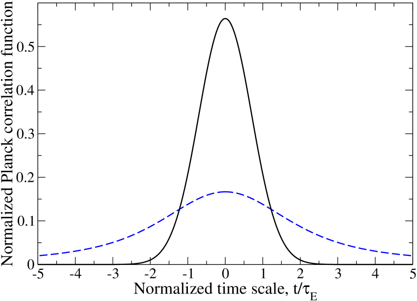
Figure 6: Correlation function of the Langevin random-force. Continuous curve refers to the normalized Planck black-body law of relation (101) and dashed curve refers to the normalized Gaussian shape $(1/\sqrt{\pi})exp(t/\tau_{\epsilon})$. Both curves look significantly broadened with respect to the classical delta-function shape, with the Planck curve exhibiting a longer tail than the Gaussian curve .Correlation function of the Langevin random-force.

Figure (6) shows the normalized correlation function associated with the Planck law (continuous curve) which is compared with a normalized Gaussian function (dashed cure). Both curves look significantly broadened with respect to the shape of the delta function corresponding to the classical condition, with the Planck correlation-function exhibiting a longer tail than that of the Gaussian function.

Figures (7) and (8) report the normalized spectra near the cut-off region associated with: (i) Planck black-body radiation law, (ii) Nyquist spectral-density with the cut-off associated with the intrinsic equivalent-circuitl of the impedance of Fig. (2) for the cases of voltage and current fluctuations, respectively. Figure (7) refers to the case of a typical metal and Fig. (8) to the case of an $n$-Si semiconductor material with a donor concentration of $N_{D}=10^{13}\ cm^{-3}$ at the same temperature of $300\ K$. For the case of a metal, owing to the significant small values of the intrinsic time scales (see the values of scattering, dielectric relaxation and plasma times reported in the figure caption) the black-body cut-off occurs at a frequency significantly lower than the values of the cut-off frequencies for the real part of the admittance or impedance spectra. (Notice the spike of the impedance spectrum at the plasma frequency). By contrast, for the case of a typical semiconductor, like $n$-type Si, owing to the significant high values of the intrinsic time scales (see the values reported in the figure caption), the black-body cut-off occurs at a frequency higher than the values of the cut-off frequencies for the real part of its admittance or impedance spectra. (Notice the absence of the spike of the impedance spectrum at the plasma frequency). We remark that Figs. (7) and (8) show that the noise spectra of a conductor, being dependent of the small-signal electrical characteristics of the material differ from that of the black-body which by contrast is a universal characteristic. In any case, the cut-off frequencies of the transport coefficients suffice to avoid the ultra-violet divergence of the voltage and current spectra for a given material. Furthermore, we notice that the Langevin equation for vacuum resistance also implies avoiding ultraviolet catastrophe for the spectral densities of fluctuations because of finite-size effects associated with the transit time between opposite contacts of the electromagnetic fields, as predicted by the energy equipartition laws for the variance of the fluctuating electromagnetic fields. Figure (6) shows the normalized correlation function associated with the Planck law (continuous curve) which is compared with a normalized Gaussian shape (dashed cure). Both curves look significantly broadened with respect to the shape of the delta function, with the Planck correlation-function exhibiting a longer tail than that of the Gaussian shape.

Figures (7) and (8) report the normalized spectra near the cut-off region associated with: (i) Planck black-body radiation law, (ii) Nyquist spectral-density with the cut-off associated with the intrinsic equivalent-circuitl of the impedance of Fig. (2) for the cases of voltage and current fluctuations, respectively. Figure (7) refers to the case of a typical metal and Fig. (8) to the case of an $n$-Si semiconductor material with a donor concentration of $N_{D}=10^{13}\ cm^{-3}$ at the same temperature of $300\ K$. For the case of a metal, owing to the significant small values of the intrinsic time scales (see the values of scattering, dielectric relaxation and plasma times reported in the figure caption) the black-body cut-off occurs at a frequency significantly lower than the values of the cut-off frequencies for the real part of the admittance or impedance spectra. (Notice the spike of the impedance spectrum at the plasma frequency). By contrast, for the case of a typical semiconductor, like n-type Si, owing to the significant high values of the intrinsic time scales (see the values reported in the figure caption), the black-body cut-off occurs at a frequency higher than the values of the cut-off frequencies for the real part of its admittance or impedance spectra. (Notice the absence of the spike of the impedance spectrum at the plasma frequency). We remark that Figs. (7) and (8) show that the noise spectra of a conductor, being dependent of the small-signal electrical characteristics of the material differ from that of the black-body which by contrast is a universal characteristic. In any case, the cut-off frequencies of the transport coefficients suffice to avoid the ultra-violet divergence of the voltage and current spectra for a given material. Furthermore, we notice that the Langevin equation for vacuum resistance also implies avoiding ultraviolet catastrophe for the spectral densities of fluctuations because of finite-size effects associated with the transit time between opposite contacts of the electromagnetic fields, as predicted by the energy equipartition laws for the variance of the fluctuating electromagnetic fields.

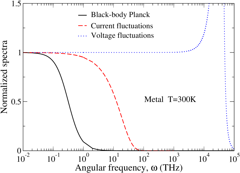
Figure 7: Noise and black-body spectra near cut-off for the case of a typical metal at $T=300\ K$. Here typical time scales are, respectively, of $\tau=10^{-2}\ ps$, $\tau_{d}=8.6\times 10^{-8}\ ps$, $\tau_{p}=2.9\times 10^{-5}\ ps$ and $\tau_{\epsilon}=7.6\times 10^{-2}\ ps$

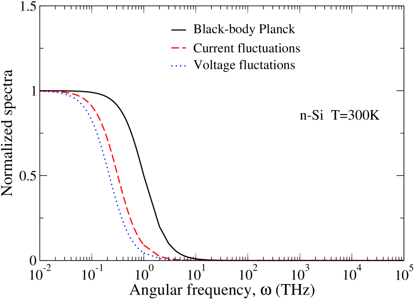
Figure 8: Noise and black-body spectra near cut-off for the case of a n-type Si sample at $T=300\ K$ with a donor concentration of $N_{D}=10^{13}\ cm^{-3}$. Here typical time scales are, respectively, of $\tau=0.24\ ps$, $\tau_{d}=4.6\ ps$, $\tau_{p}=1.1\ ps$, and $\tau_{\epsilon}=7.6\times 10^{-2}\ ps$.

VII.1 Fluctuation dissipation theorem for a gas of photons

For a gas of photons the number of quasi-particles is not conserved in time and thus the chemical potential is zero. Furthermore the energy dispersion is

$$\epsilon_{k}=\hbar\omega,$$ (102)

and the density of states $g(\epsilon_{k})$ is

$$g(\epsilon_{k})=V_{0}\frac{8\pi}{c^{3}}f^{2}$$ (103)

Accordingly, by definition it is

$$\frac{\overline{N_{p}}}{V_{0}}=\frac{8\pi\Gamma(3)\zeta(3)}{c^{3}h^{3}}\ (K_{B}T)^{3}=(2.02\ 10^{7})\ T^{3}\ (m^{-3})$$ (104)

with $\Gamma(3)\zeta(3)=\int_{0}^{\infty}x^{2}/(e^{x}-1)dx=2.404$.

$$\frac{\overline{\epsilon_{tot}}}{V_{0}}=\frac{8\pi\Gamma(4)\zeta(4)}{c^{3}h^{3}}\ (K_{B}T)^{4}=7.57\ 10^{-16}\ T^{4}\ (Jm^{-3})$$ (105)

with $\overline{\epsilon_{tot}}$ the internal average-energy in the considered volume, $\Gamma(4)\zeta(4)=\pi^{4}/15=6.49$, and

$$\overline{\epsilon_{mode}}=\frac{\overline{\epsilon_{tot}}}{\overline{N_{p}}}=\ 2.7\ K_{B}T$$ (106)

with $\overline{\epsilon_{mode}}$ the average energy per photon mode, notice that its value is slightly less than that of the classical case per full relativistic massive-particle of $3\ K_{B}T$ due to photon Bose-Einstein distribution, and much less than that of the degenerate case per full degenerate Fermions of $3/5(\mu_{0})$.

Since photons are relativistic particles, in vacuum it is

$$\overline{v^{2^{\prime}}_{z}}=c^{2}$$ (107)

$$\overline{\delta N^{2}_{p}}=V_{0}\frac{8\pi}{c^{3}h^{3}}\ (K_{B}T)^{3}\int_{0}^{\infty}\frac{x^{2}e^{x}}{(e^{x}-1)^{2}}dx=1.37\overline{N_{p}}$$ (108)

Notice, that the super Poissonian value, with a Fano factor $\overline{\delta N_{p}^{2}}/\overline{N_{p}}=1.37$ due to Bose-Einstein distribution, should be compared with the value $\overline{\delta N^{2}}/\overline{N}=1$ of classical massive-particle statistics and the value $\overline{\delta N^{2}}/\overline{N}=0$ of full-degenerate massive-particle statistics at $T=0$.

The duality property of the noise sources of a photon gas writes

$$\overline{\delta v_{d}^{2}}=c^{2}\frac{\overline{\delta N_{p}^{2}}}{{\overline{N}_{p}}^{2}}=\frac{1.37c^{2}}{\overline{N_{p}}},$$ (109)

that implies the reciprocity relations

$$\overline{\delta v_{d}^{2}}\ {\overline{N_{p}}}^{2}=\overline{\delta N_{p}^{2}}\ \overline{v^{2^{\prime}}_{x}}=1.37c^{2}{\overline{N_{p}}}=cost\ T^{3}$$ (110)

We conclude, that for the photon gas the microscopic noise source comes from the fluctuations of the photon number only, and its average value is proportional to the third power of the temperature. At zero temperature fluctuations vanish apart from the presence of zero-point contribution which can be considered associated with Bose-Einstein condensation of the photons ground state and which is responsible of the Casimir effect. However the Casimir effect does not produce fluctuations by itself but a macroscopic quantum-energy associated with the spatial confinement of the physical system.

For the diffusion coefficient and the plasma mobility of the photon gas we find

$$D=\overline{v^{2^{\prime}}_{x}}\tau=cL$$ (111)

$$\mu^{2}_{P}=\frac{q^{2}\tau_{P}^{2}}{m^{2}}=\alpha 4\pi\epsilon_{0}\ \hbar c\frac{L^{2}}{c^{2}}\frac{c^{4}}{(\hbar\omega)^{2}}=\frac{4\pi\epsilon_{0}\hbar c}{137}\frac{L^{2}c^{2}}{(\hbar\omega)^{2}}$$ (112)

with $\alpha=1/137$ the fine structure constant, that has been used to convert the electron charge into the vacuum charge, and $\hbar\omega$ the photon relativistic mass, that replaces the electron mass.

VIII Conclusions

This review presents a revisitation of the fluctuation dissipation theorem (FDT)that from an historical point of view is traced back to the discovery of the fundamental laws governing the black-body radiation spectrum. The main objective of the paper is to further stress the unifying microscopic interpretation of the interaction between radiation and matter, and of electrical noise in particular, given by this theorem. Main points that received new insights in specific parts of the paper are briefly summarized in the following list.

1 - The zero-point energy term, that is present in the quantum formulation of FDT due to Callen and Welton callen51 , does not contribute to electrical fluctuations. By contrast, it is responsible of the Casimir force, a pure quantum-mechanical macroscopic effect, that by implying a mechanical instability of the physical system, should be exactly balanced by a reaction force to recover stability, a necessary condition to detect electrical fluctuations. The reaction force can be absorbed by the elastic properties of the environment associated with the physical system.

2 - The role of the different statistical ensembles (microcanonical, canonical and grand-canonical) in the formulation of the FDT has been analyzed. Accordingly, the microscopic noise sources associated with the properties of the medium inside the physical system have been individuated.

3 - We have identified the intrinsic equivalent-circuit for the impedance (admittance) model of the physical system appropriate to describe the relaxation of voltage (current) fluctuations and thus the intrinsic bandwidth of the classical noise spectral densities described by Nyquist theorem.

4 - The appropriate Langevin equations for the current or voltage operation modes used to detect noise spectra have been formulated and solved.

5 - The duality and reciprocity relations between microscopic noise sources responsible of the so-called thermal agitation of electric charge in conductors have been investigated. Here, fluctuations of the total number of carriers inside the physical system are shown to be responsible of current fluctuations detected in the external short circuit, while fluctuations of the carrier drift-velocity are found to be responsible of the voltage fluctuations detected in the open external circuit. In essence, the duality relations imply a generalized Biot-Savart law converting the variance of current fluctuations with the variance of magnetic field fluctuations, see Eq. (91), and a generalized Ohm law converting the variance of drift-velocity fluctuations with the variance of electric field fluctuations, see Eq. (92).

6 - The FDT has been generalized to the cases of: (i) the ballistic transport regime of charge-carrier dynamics, (ii) the vacuum and, (iii) the quantum case when $K_{B}T$ is substituted by the Planck spectrum, as originally suggested by Nyquist nyquist28 . We noticed, that the noise spectra associated with current and voltage fluctuations of a conductor are intrinsic characteristics of the material under study, and thus differ from the black-body spectrum that by contrast is a universal property.

7 - The validity of the FDT has been extended to the case of fractional statistics.

8 - The FDT has been applied to the case of a photon gas where noise source has been associated with the fluctuations of the instantaneous photon number inside the physical system.

References

- (1) H. Nyquist, Thermal agitation of electric charge in conductors, Phys. Rev. 32 (1928) 110-113.
- (2) D. ter Haar, Elements of Statistical Mechanics (Butterworth-Heinemann Ltd, Oxford, 1955).
- (3) G. Parisi, Planck’ s legacy to statistical mechanics, arXiv:cond-mat/0101293 (18-I20-01) (2001).
- (4) L. Boya, The thermal radiation formula of Planck, 12 2 (2004). arxiv.org/pdf/physics/0402064.pdf.
- (5) G. Kirchhoff, On the relation between the radiating and absorbing powers of different bodies for light and heat, Phil. Mag. S- 4. Vol. 20, No. 180 (1860) p. 275.
- (6) A. Einstein, Über die von der molekularkinetischen Theorie der Wärme geforderte Bewegung von in ruhenden Flüssigkeiten suspendierten Teilchen (On the movement of small particles suspended in stationary liquids required by the molecular-kinetic theory of heat), Annalen der Physik 322 (8) (1905) 549-560.
- (7) P. Langevin, Sur la theorie du mouvement brownien (On the theory of Brownian motion), C. R. Acad. Sci. Paris 14 (1908) 530-533.
- (8) M. Planck, Uber die begrundung des gesetzes der schwarzen strahlung (On the grounds of the law of black body radiation), Annalen der Physik 6 (1912) 642.
- (9) J.B. Johnson, Thermal agitation of electricity in conductors, Nature 119 (1927) 50-51; ibidem Phys. Rev. 32 (1928) 97-109.
- (10) L. Onsager, Reciprocal relations in irreversible processes. I. Phys. Rev. 37, (1931) 405-426; ibidem, Reciprocal relations in irreversible processes. II. Phys. Rev. 38 (1931) 2265-2279.
- (11) H. Casimir, On the attraction between two perfectly conducting plates, Proc. K. Ned. Akad. Wet. 51 (1948) 793-795.
- (12) H.B. Callen and T.A. Welton, Irreversibility and generalized noise, Phys. Rev. 83 (1951) 34-40.
- (13) R. Kubo, Statistical-mechanical theory of irreversible processes. I., Phys. Soc, Japan 12 (1957) 570-586; ibidem, The fluctuation-dissipation theorem, Rep. Prog. Phys. 29 (1966) 255-284.
- (14) Marcus V.S. Bonanca, Fluctuation-dissipation theorem for the microcanonical ensemble, Phys. Rev. E 78 (2008) 031107.
- (15) L. Reggiani, E. Alfinito and T. Kuhn, Duality and reciprocity of fluctuation-dissipation relations in conductors, Phys. Rev. E 94 (2016) 032112.
- (16) L. Reggiani and E. Alfinito, The puzzling of zero-point energy contribution to black-body radiation spectrum: The role of Casimir force, Fluct. Noise Lett. 16 (2017) 1771002 (6 pages).
- (17) G W. Ford, J.T. Lewis, and R F. O’ Connell, Quantum Langevin equation, Phys. Rev. A 37 (1988) 4419-4428.
- (18) M. Planck, Ueber das Gesetz der Energieverteilung im Normalspectrum (On the law of distribution of energy in the normal spectrum), Annalen der Physik 4 (1901) 553-563.
- (19) M. Kardar and R. Golestanian, The ‘friction’ of vacuum, and other fluctuation-induced forces, Rev. Mod. Phys. 71 (1999) 1233-1247.
- (20) P.A.M. Dirac, Discussion of the infinite distribution of electrons in the theory of the positron, Proc. Camb. Phil. Soc. 30 (1934) 150-163.
- (21) K. Milton, The Casimir Efect: Physical Manifestations of Zero-Point Energy, World Scientific Publishing, Singapore (2001).
- (22) A. Edery, Casimir forces in Bose-Einstein condensate: finite size effects in three dimensional rectangular cavities, J. Stat. Mech.: Theory and Experiments 06 (2006) P06007.
- (23) F. Schmidt and H. Diehl, Crossover from attractive to repulsive Casimir force and vice versa, Phys. Rev. Lett. 101 (2008) 10601-10604.
- (24) G. Auletta, M. Fortunato, and G. Parisi, Quantum Mechanics, Cambridge University (2009).
- (25) J. Lebowitz and E. Liebf, Existence of thermodynamics for real matter with Coulomb forces, Phys. Rev. Lett. 13 (1969) 631-634.
- (26) C. Kittel, Introduction to Solid State Physics, John Wiley and Sons, (2004).
- (27) S. Kogan, Electronic Noise and Fluctuations in Solids, Cambridge University Press (1996).
- (28) I. Prigogine and D. Kondepudi, Modern Thermodynamics: from Heat Engines to Dissipative Sructures, Wiley (2014).
- (29) D.N. Zubarev, Nonequilibium Statistical Thermodinamics, Nauka, Moscow (1971).
- (30) L. Landau and E. Lifshitz, Statistical Physics, Addison Wesley Reading, Mass (1974).
- (31) W. Shockley, Currents to conductors induced by a moving point charge, J. Appl. Phys. 9 (1938) 635-636.
- (32) S. Ramo, Currents induced by electron motion, Proc. IRE 27 (1939) 584-585.
- (33) B. Pellegrini, Electric charge motion, induced current, energy balance, and noise, Phys. Rev. B34 (1986) 5921-5924.
- (34) B. Pellegrini, Extension of the electrokinematics theorem to the electromagnetic field and quantum mmchanics, Nuovo Cimento D 15 (1993) 855-879; ibidem Elementary applications of quantum-electrokinematics theorem, (1993) 881-896.
- (35) L. Reggiani, All the colors of noise, in 22nd International Conference on Noise and Fluctuations (ICNF) IEEE 10.1109/ICNF.2013.6578874 (2013) 1-6.
- (36) D.A. McQuarrie, Statistical Mechanics, Harper and Row Publisher, New York (1976).
- (37) S. Gantsevich, R. Katilius and V. Gurevich, Theory of fluctuations in nonequilibrium electron gas, Rivista Nuovo Cimento 2 (1979) 1-87.
- (38) Y. Imry and R. Landauer, Conductance viewed as transmission, Rev. Mod. Phys. 71 (1999) S306-S312.
- (39) A. Greiner, L. Reggiani, T. Kuhn and L. Varani, Carrier kinetics from the diffusive to the ballistic regime: linear response near thermodynamic equilibrium, Semicond. Sci. Technol. 15 (2000) 1071-1081.
- (40) Yu. L. Klimontovich, Fluctuation-dissipation relations. Role of the finiteness of the correlation time. Quantum generalization of Nyquist’s formula, Sov. Phys. Usp. 30 (1987) 154-167.
- (41) P.T. Landsberg, Quantum statistics of closed and open systems, Phys. Rev. 93 (1954) 1170-1171.
- (42) J. Dunning-Davis, Particle-number fluctuations, Nuovo Cimento 57B, (1968) 315-316.
- (43) B.I. Halperin, Statistics of quasiparticles and the hierarchy of fractional quantized Hall states, Phys. Rev. Lett. 52 (1984) 1583-1586.
- (44) Y.S. Wu, Statistical distribution for generalized ideal gas of fractional-statistics particles, Phys. Rev. Lett. 73 (1995) 922-925.
- (45) C.W. Gardiner and P. Zoller, Quantum Noise, Springer-Verlag, Berlin (2000).