Squeezed in three dimensions, moving in two: Hydrodynamic theory of 3D incompressible easy-plane polar active fluids

Abstract

We study the hydrodynamic behavior of three dimensional (3D) incompressible collections of self-propelled entities in contact with a momentum sink in a state with non-zero average velocity, hereafter called 3D easy-plane incompressible polar active fluids. We show that the hydrodynamic model for this system belongs to the same universality class as that of an equilibrium system, namely a special 3D anisotropic magnet. The latter can be further mapped onto yet another equilibrium system, a DNA-lipid mixture in the sliding columnar phase. Through these connections we find a divergent renormalization of the damping coefficients in 3D easy-plane incompressible polar active fluids, and obtain their equal-time velocity correlation functions.

Diverse distinct systems can share identical large-distance, scale invariant properties. This “universality”, which occurs when the distinct systems share common symmetries, can link seemingly disparate areas of physics. In this paper, we reveal such a surprising connection between two such areas: Active matter Active and self-assembly of biomimetic material. Specifically, we demonstrate that a particular three dimensional (3D) phase of self-propelled, incompressible agents - namely, what we call an “incompressible easy-plane active fluid” can exhibit precisely the same scaling behavior as an equilibrium mixture of DNA and cationic lipids in a hypothesized phase known as the “sliding columnar” phase Column1 ; Column2 ; Column (Fig. 1).

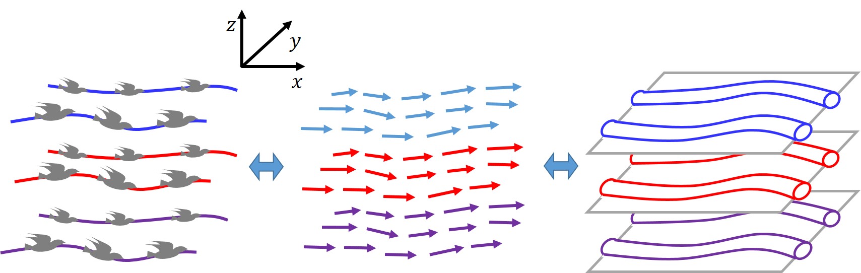
Figure 1: A schematic illustrating that an incompressible flock with an easy-plane of flying, an easy-plane magnet, and a sliding columnar phase have identical equal-time statistics in the hydrodynamic limit: the fluctuations of the flow lines, magnetic lines, and the columns share the same scaling behavior.

An “incompressible easy-plane active fluid” is a collection of self-propelled entities, which could be, e.g., living creatures like bacteria, or synthetic self-propelled objects like Janus particles Janus or “Quinke rotators” Bartolo . The term “active” refers in this context to their self-propulsion. “Incompressible” means that we consider specifically systems in which these self-propelled particles move in such a way that they do not change their density, either because they are tightly packed, so that no space is available for them to change their density, or because of long-ranged interactions, like the ions in a plasma. By “easy-plane”, we mean systems in which the motion of these entities is preferentially parallel to some plane (note that the collection itself fills a three dimensional space).

In its “ordered state”, on which we focus here, the collection of moving entities has a non-zero average velocity in the thermodynamic ($N\rightarrow\infty$, where $N$ is number of self-propelled entities in the system) limit.

The “sliding columnar phase” of cationic-lipid DNA complexes is a conjectured phase in which nearly straight DNA molecules are confined between a set of 3D space filling lipid layers. The DNA align with each other, both in a given “layer”, and between layers. In addition, there are positional interactions between neighbors within a given layer, but only orientational interactions between layers.

To establish the connection between the two very different systems we’ve just described, we first formulate a generic hydrodynamic theory of easy-plane polar active fluids. Using a dynamical renormalization group (DRG) analysis, we then show that this model can be mapped onto the time-dependent-Ginsburg-Landau (TDGL) model of an equilibrium, divergence-free 3D magnet with an easy-plane. We then focus on the static (equal-time) properties and use a static equilibrium RG analysis to connect our magnet to an equilibrium system in the sliding columnar phase. The connections between these theoretical models are illustrated in Fig. 1. Through these connections we are able to go beyond linear hydrodynamics and calculate the exact scaling of the equal-time velocity correlation function of our active system, which is radically altered by non-linearities.

Specifically, we find the equal-time velocity fluctuations in the active fluid are proportional to the orientational fluctuations of the DNA strands in the sliding columnar phase. Since the latter are known to be bounded Column1 ; Column2 ; Column , we can conclude that velocity fluctuations are bounded in the active fluid as well, implying that the ordered phase with non-zero average velocity exists. Furthermore, we can use the mapping to show that the connected part of the velocity correlation function in the ordered phase has the following equal-time scaling behavior at large distances (i.e., $x\gg\xi_{x}$, $z\gg\xi_{z}$, or $y\gg\xi_{y}$):

$$\langle\left[\mathbf{v}(0,t)-\mathbf{v}_{0}\right]\cdot\left[\mathbf{v}(\mathbf{r},t)-\mathbf{v}_{0}\right]\rangle\sim$$

$$\left\{\begin{array}[]{ll}{\left(\ln{X}\right)^{1\over 4}\ln\left(\ln X\right)\over\left(x\Lambda\right)^{2}}\,,&X\gg Y^{1\over 2}\left(\ln{Y}\right)^{5\over 16},Z\left(\ln{Z}\right)^{1\over 8}\\ {\left(\ln{Y}\right)^{-{3\over 8}}\over|y|\Lambda}\,,&Y\gg X^{2}\left(\ln{X}\right)^{-{5\over 8}},Z^{2}\left(\ln{Z}\right)^{-{3\over 8}}\\ {1\over\left(z\Lambda\right)^{2}}\,,&Z\gg X\left(\ln{X}\right)^{-{1\over 8}},Y^{1\over 2}\left(\ln{Y}\right)^{3\over 16}\end{array},\right.$$ (4)

where ${\mathbf{r}}=(x,y,z)$, $\xi_{x,y,z}$ are some non-universal lengths which we calculate in SM , $\Lambda$ is the ultra-violet cutoff, $X\equiv{|x|\over\xi_{x}}$, $Y\equiv{|y|\over\xi_{y}}$, $Z\equiv{|z|\over\xi_{z}}$, $\mathbf{v}_{0}$ is the average velocity of the system taken to be along the $x$-direction, and the easy plane is denoted as the $xy$-plane. At short distances (i.e., $|x|\ll\xi_{x}$, $|y|\ll\xi_{y}$, and $|z|\ll\xi_{z}$) (4) reduces to that of linear theory, all the logarithms becoming 1. Note that the crossover lengths $\xi_{x}$, $\xi_{z}$ and $\xi_{y}$ can be very large, since they are exponential functions of the parameters - in particular, of the noise strength defined below. Therefore, to observe the logarithms in (1) in experiments or simulations, very large system sizes may be required. For smaller systems, the correlations behave as in (1), but with all of the logarithms replaced by constants.

To formulate a hydrodynamic theory of 3D incompressible easy-plane polar active fluids, we start with the generic equation of motion (EOM) of compressible active fluids TT1 ; TT3 ; TT4 ; rean , with an addition linear damping term that forces the velocity field to lie preferentially on the easy plane ($xy$-plane):

$$\partial_{t}\rho = -\nabla\cdot(\mathbf{v}\rho)\ ,$$ (5)

$$\partial_{t}\mathbf{v} = -2gv_{z}\hat{{\bf z}}-\lambda_{1}(\mathbf{v}\cdot\nabla)\mathbf{v}-\lambda_{2}(\nabla\cdot\mathbf{v})\mathbf{v}-\lambda_{3}\nabla(v^{2})$$ (6)

$$+U\mathbf{v}-\nabla P-\mathbf{v}\left(\mathbf{v}\cdot\nabla P_{2}\right)+\mu_{{\rm B}}\nabla(\nabla\cdot\mathbf{v})$$

$$+\mu_{\rm T}\nabla^{2}\mathbf{v}+\mu_{2}(\mathbf{v}\cdot\nabla)^{2}\mathbf{v}+{\mathbf{f}}\,.$$

Here $\mathbf{v}(\mathbf{r},t)$, and $\rho(\mathbf{r},t)$ are respectively the coarse grained continuous velocity and density fields, and $(-2gv_{z}\hat{{\bf z}})$ is a symmetry breaking damping term that makes the velocity field tend to lie parallel to the $xy$-plane. The random driving force $\mathbf{f}$ is assumed to be Gaussian with white noise correlations:

$$\langle f_{m}(\mathbf{r},t)f_{n}(\mathbf{r}^{\prime},t^{\prime})\rangle=2D\delta_{mn}\delta^{d}(\mathbf{r}-\mathbf{r}^{\prime})\delta(t-t^{\prime})$$ (7)

where the “noise strength” $D$ is a constant parameter of the system, and $m$, $n$ denote Cartesian components. Note that since our intention is to study systems that are not momentum conserving, these chosen statistics do not conserve momentum, in contrast to thermal fluids (e.g., Model A in FNS ).

All of the parameters $\lambda_{i}\ (i=1\to 3)$, $U$, the “damping coefficients” $\mu_{\rm B,T,2}$, the “isotropic pressure” $P(\rho,v)$ and the “anisotropic pressure” $P_{2}(\rho,v)$ are, in general, functions of the density $\rho$ and the magnitude $v\equiv|\mathbf{v}|$ of the local velocity.

Since we are interested in the ordered state (which we will show to exist later), we assume the $U$ term makes the local $\mathbf{v}$ have a nonzero magnitude $v_{0}$ in the steady state, by the simple expedient of having $U>0$ for $v<v_{0}$, $U=0$ for $v=v_{0}$, and $U<0$ for $v>v_{0}$. We treat fluctuations by expanding $\mathbf{v}$ around $v_{0}\hat{\bf x}$, thus defining $\mathbf{u}(\mathbf{r},t)$ as the small fluctuation in the velocity field about this mean:

$$\mathbf{v}(\mathbf{r},t)=(v_{0}+u_{x}(\mathbf{r},t))\hat{\bf x}+u_{y}(\mathbf{r},t)\hat{\bf y}+u_{z}(\mathbf{r},t)\hat{\bf z}\ .$$ (8)

We now go to the incompressible limit by taking the isotropic pressure $P$ to be extremely sensitive to departures from the mean density $\rho_{0}$, so that it suppresses density fluctuations extremely effectively. Therefore, changes in the density are too small to affect $U(\rho,v)$, $\lambda_{1,2,3}(\rho,v)$, $\mu_{{\rm B},{\rm T},2}(\rho,v)$, and $P_{2}(\rho,v)$. As a result, all of them effectively become functions only of the speed $v$; their $\rho$-dependence drops out since $\rho$ is essentially constant. Another consequence of the suppression of density fluctuations by the isotropic pressure $P$ is that the continuity equation (5) reduces to the condition

$$\nabla\cdot\mathbf{v}=0\ .$$ (9)

In particular, the $\lambda_{2}$ and $\mu_{B}$ terms vanish due to this condition (9).

Models of incompressible active fluids as defined here are rich in physics: incompressible active fluids whose their motion is not confined to an easy plane, undergo a critical order-disorder transition that exhibits novel universal behavior us1 ; and in the ordered phase in 2D, the system can be mapped onto the (1+1)D Kardar-Parisi-Zhang surface growth model us2 . With the easy-plane restriction considered here, we shall see that the ordered phase can be mapped onto an equilibrium soft matter system.

With the incompressibility condition (9) taken into account and using (8) in (6), we find

$$\partial_{t}\mathbf{u} = -2gu_{z}\hat{{\bf z}}-\lambda^{0}_{1}v_{0}\partial_{x}\mathbf{u}-\lambda^{0}_{1}(\mathbf{u}\cdot\nabla)\mathbf{u}$$ (10)

$$-2\alpha\left(u_{x}+{u_{y}^{2}\over 2v_{0}}\right)\hat{{\bf x}}-\nabla P$$

$$+\left[\mu^{0}_{\rm T}\left(\partial_{y}^{2}+\partial_{z}^{2}\right)+\mu_{x}\partial_{x}^{2}\right]\mathbf{u}+{\mathbf{f}}\,.$$

where we have defined $\alpha\equiv{1\over 2}{dU\over dv}\big{|}_{v=v_{0}}$, $\mu_{x}\equiv\mu_{\rm T}^{0}+\mu^{0}_{2}v_{0}^{2}$, and have absorbed a term $W(v)$ into the pressure $P$, where $W(v)$ is derived from $\lambda_{3}(v)$ by solving ${1\over 2v}{dW\over dv}=\lambda_{3}(v)$. The superscript “0” means that the $v$-dependent coefficients are evaluated at $v=v_{0}$. In the above EOM, we have also omitted “obviously” irrelevant terms in the sense discussed in us2 .

We can further simplify the EOM by making a Galilean transformation to a “pseudo-co-moving” co-ordinate system moving in the direction $\hat{\bf x}$ of mean flock motion at speed $\lambda^{0}_{1}v_{0}$ to eliminate the “convective term” $\lambda^{0}_{1}v_{0}\partial_{x}\mathbf{u}$ from the right hand side of (10); this leaves us with our final simplified form for the EOM:

$$\partial_{t}\mathbf{u} = -2gu_{z}\hat{{\bf z}}-\lambda^{0}_{1}(\mathbf{u}\cdot\nabla)\mathbf{u}-2\alpha\left(u_{x}+{u_{y}^{2}\over 2v_{0}}\right)\hat{{\bf x}}$$ (11)

$$-\nabla P+\left[\mu^{0}_{\rm T}\left(\partial_{y}^{2}+\partial_{z}^{2}\right)+\mu_{x}\partial_{x}^{2}\right]\mathbf{u}+{\mathbf{f}}\,.$$

Since both $u_{x}$ and $u_{z}$ are “massive”, because of the $2gu_{z}$ and $2\alpha u_{x}$ terms, respectively, we expect the fluctuations of $u_{y}$ to dominate over those of $u_{x,z}$. We therefore focus on the EOM of $u_{y}$. We obtain this by Fourier transforming (11) in space at wavevector $\bf{q}$ and eliminating the pressure term by acting on both sides of the equations with the transverse projection operator $P_{lm}(\mathbf{q})=\delta_{lm}-q_{l}q_{m}/q^{2}$, and looking at the $l=y$ component of the resulting equation. The linearized EOM of $u_{y}$ thereby becomes

$$\partial_{t}u_{y}(\mathbf{q},t) = P_{ym}(\mathbf{q})f_{m}(\mathbf{q},t)-\Gamma(\mathbf{q})u_{y}(\mathbf{q},t)$$ (12)

$$+2\alpha{q_{x}q_{y}\over q^{2}}u_{x}(\mathbf{q},t)+2g{q_{y}q_{z}\over q^{2}}u_{z}(\mathbf{q},t)\ ,$$

where we’ve defined $\Gamma(\mathbf{q})\equiv\mu_{x}q_{x}^{2}+\mu_{\rm T}^{0}\left(q_{y}^{2}+q_{z}^{2}\right)$.

To proceed further, we perform a DRG analysis by first rescaling the coordinates and fluctuating fields:

$$x \mapsto {\rm e}^{\ell}x\,,~{}y\mapsto{\rm e}^{\zeta_{y}\ell}y\,,~{}z\mapsto{\rm e}^{\zeta_{z}\ell}z\,,~{}t\mapsto{\rm e}^{w\ell}t\,,$$ (13)

$$u_{y} \mapsto {\rm e}^{\chi_{y}\ell}u_{y}\,,$$ (14)

$$u_{x} \mapsto {\rm e}^{\chi_{x}\ell}u_{x}={\rm e}^{\left(\chi_{y}+1-\zeta_{y}\right)\ell}u_{x}\,,$$ (15)

$$u_{z} \mapsto {\rm e}^{\chi_{z}\ell}u_{z}={\rm e}^{\left(\chi_{y}+\zeta_{z}-\zeta_{y}\right)\ell}u_{z}\,,$$ (16)

where we’ve enforced the equalities in (15) and (16) to maintain the form of the incompressibility condition (9).

Applying these rescalings (13-16) to the linear EOM of $u_{y}$ (12), we find that the parameters rescale as

$$\mu_{x}\mapsto{\rm e}^{\left(w-2\right)\ell}\mu_{x}\ ,\ \ \ ,\ \ \ \mu_{\rm T}^{0}\mapsto{\rm e}^{\left(w-2\zeta_{z}\right)\ell}\mu_{\rm T}^{0}\ ,$$ (17)

$$\alpha\mapsto{\rm e}^{\left(w-2\zeta_{y}+2\min(1,\zeta_{y},\zeta_{z})\right)\ell}\alpha\ ,$$ (18)

$$g\mapsto{\rm e}^{\left(w-2\zeta_{y}+2\min(1,\zeta_{y},\zeta_{z})\right)\ell}g\ ,$$ (19)

$$D\mapsto{\rm e}^{\left(w-2\chi_{y}-\zeta_{y}-\zeta_{z}-1\right)\ell}D\,.$$ (20)

where the ${\rm min}(1,\zeta_{y},\zeta_{z})$ appears because, in the limit $\ell\to\infty$, the values of $\zeta_{y,z}$ determine which component $q_{x,y,z}$ dominates the $q^{2}$’s that appear in (12).

We now choose the rescaling exponents $w$, $\zeta_{y,z}$, and $\chi_{y}$ so as to keep the size of the fluctuations in the field $\mathbf{u}$ fixed upon rescaling. This is accomplished by keeping $\alpha$, $g$, $\mu_{x}$, $\mu_{\rm T}^{0}$, and $D$ fixed. From the rescalings just found, this leads to four simple linear equations in the four unknown exponents $w$, $\zeta_{y,z}$, and $\chi_{y}$; solving these, we find

$$w=\zeta_{y}=2\,,~{}\zeta_{z}=1\,,~{}\chi_{{}_{y}}=-1\,.$$ (21)

With these exponents in hand, we can now assess the importance of the non-linear terms in the full EOM for $u_{y}$ at long length scales, simply by looking at how their coefficients rescale. We find that all the non-linear terms whose coefficients are proportional to $\alpha$ are “marginal”, that is, the coefficients of these terms remain fixed upon rescaling. However, the last remaining non-linear term is “irrelevant” because its coefficient gets smaller upon rescaling: $\lambda^{0}_{1}\mapsto{\rm e}^{-\ell}\lambda^{0}_{1}$. Hence, this term will not affect the long-distance behavior, and can be dropped from the problem.

Now we come back to Eq. (11) and drop the “irrelevant” $\lambda_{1}^{0}$ non-linear term. The reduced EOM becomes identical to the TDGL model:

$$\frac{\partial u_{m}}{\partial t}=-\frac{\delta H}{\delta u_{m}}+f_{m}\ ,$$ (22)

where $\mathbf{f}$ is the thermal noise whose statistics are described by Eq. (7) with $D=k_{B}T$, and with the Hamiltonian

$$H = \frac{1}{2}\int{\rm d}^{3}r\Bigg{\{}2\alpha\left(u_{x}+{u_{y}^{2}\over 2v_{0}}\right)^{2}+2gu_{z}^{2}$$ (23)

$$+\left(\mu_{x}-\mu_{\rm T}^{0}\right)(\partial_{x}u_{y})^{2}+\mu_{\rm T}^{0}|\nabla u_{y}|^{2}\Bigg{\}}\,,$$

where we have $P(\mathbf{r})$ as the Lagrange multiplier employed to enforce the divergence-free (incompressibility) constraint $\nabla\cdot\mathbf{u}=0$. One can now straightforwardly check that the TDGL model equation in (22) does lead to the EOM (11) without the “irrelevant” $\lambda_{1}^{0}$ non-linear term.

This mapping between a nonequilibrium active fluid model and a “divergence-free” easy-plane equilibrium magnet model allows us to investigate the fluctuations in our original active fluid model by studying the partition function of the equilibrium model (23). Since the magnetization prefers to point parallel to the $xy$ plane, the fluctuations of $u_{z}$ are expected to be much smaller than those of $u_{x,y}$. We here assume that the fluctuations in $u_{z}$ become negligible upon coarse-graining, i.e., $\lim_{\ell\rightarrow\infty}g=\infty$. We will justify this assumption self-consistently later.

With the elimination of $u_{z}$ (due to the divergence of $g$ upon RG transformation), we can now introduce the streaming function $h$ to enforce the incompressibility condition:

$$u_{x}=-v_{0}\partial_{y}h\ \ \ ,\ \ \ u_{y}=v_{0}\partial_{x}h\ .$$ (24)

Since this construction guarantees that the incompressibility condition $\mathbf{\nabla}\cdot\mathbf{u}=\partial_{x}u_{x}+\partial_{y}u_{y}=0$ is automatically satisfied (once we set $u_{z}=0$), there is no constraint on the field $h(\mathbf{r})$.

Substituting (24) into the Hamiltonian (23), it becomes (ignoring irrelevant terms like $(\partial_{x}\partial_{y}h)^{2}$, which is irrelevant compared to $(\partial_{y}h)^{2}$ because it involves two extra $x$-derivatives)

$$H_{s}={1\over 2}\int d^{3}r\left[B\left(\partial_{y}h-{(\partial_{x}h)^{2}\over 2}\right)^{2}\right.$$

$$\left.+K_{xx}(\partial^{2}_{x}h)^{2}+K_{xz}(\partial_{x}\partial_{z}h)^{2}\right]\ ,$$ (25)

where $B=2\alpha v_{0}^{2}$, $K_{xx}=\mu_{x}$, and $K_{xz}=\mu_{\rm T}^{0}$. This Hamiltonian is exactly the elasticity theory for the sliding columnar phase Column1 ; Column2 ; Column , with columns oriented along $x$, sandwiched between rigid plates which stack along $z$, fluctuating with displacements $h$ restricted along $y$ Column (see Fig. 1). In the sliding columnar phase, there are interactions between the orientations of the columns in different layers but none between the positions. The elastic coefficients $B$, $K_{xx}$, and $K_{xz}$ are respectively the compression, bend, and twist moduli footnote1 .

It has been shown that the anharmonic terms in (25) lead to an infinite renormalization of the elastic constants Column , as also happens in the 3D smectic phase GP . Specifically, in the long wavelength limit (i.e., $|q_{x,y,z}|<\xi_{x,y,z}$, where $\xi_{x,y,z}$ are non-universal lengths which we estimate in SM ), the compression modulus vanishes logarithmically and the bend and twist moduli diverge logarithmically according to

$$K_{xz}(\mathbf{q})\sim K_{xx}^{\frac{1}{2}}(\mathbf{q})\sim B^{-\frac{1}{3}}(\mathbf{q})\sim|\ln q|^{\frac{1}{4}}\,.$$ (26)

In terms of the coefficients of the active fluid model we have

$$\mu_{\rm T}^{0}(\mathbf{q})\sim\mu_{x}^{\frac{1}{2}}(\mathbf{q})\sim\alpha^{-\frac{1}{3}}(\mathbf{q})\sim|\ln q|^{\frac{1}{4}}\,.$$ (27)

Using these renormalized parameters in our effective equilibrium model (23) we can obtain the full equal-time correlation function for our original problem SM :

$$\langle\mathbf{u}(\mathbf{q})\cdot\mathbf{u}(\mathbf{q}^{\prime})\rangle$$

$$={\left(2\pi\right)^{3}D\left[2\alpha(\mathbf{q})q_{z}^{2}+g\left(q_{x}^{2}+q_{y}^{2}\right)\right]\delta(\mathbf{q}+\mathbf{q}^{\prime})\over\left[\mu_{x}(\mathbf{q})q_{x}^{2}+\mu_{\rm T}^{0}(\mathbf{q})q_{z}^{2}\right]\left[2\alpha(\mathbf{q})q_{z}^{2}+gq_{x}^{2}\right]+2g\alpha(\mathbf{q})q_{y}^{2}}~{},$$

(28)

where we have neglected terms which have higher powers in $q$ than the present ones in the numerator. Note that given the form of the above correlation function, we can now also conclude that the real space fluctuations $\langle u^{2}(\mathbf{r})\rangle\propto\int{\rm d}^{3}\mathbf{q}\langle|\mathbf{u}(\mathbf{q})|\rangle$ is finite, thus implying the existence of long-ranged order in the divergence-free easy-plane magnet, as well as in our incompressible active fluid model.

Given the logarithmic corrections in (26), we will now justify the divergence of $g$ in the Hamiltonian (23) upon RG transformation, and thus the neglect of $u_{z}$. Specifically, in terms of the re-scalings in Eqs (13)–(16), the RG flow equations are:

$${{\rm d}\ln\alpha\over{\rm d}\ell} = 2\chi_{y}+3-\zeta_{y}+\zeta_{z}-\eta_{\alpha}\,,$$ (29)

$${{\rm d}\ln g\over{\rm d}\ell} = 2\chi_{y}+1-\zeta_{y}+3\zeta_{z}\,,$$ (30)

$${{\rm d}\ln\mu_{x}\over{\rm d}\ell} = 2\chi_{y}-1+\zeta_{z}+\zeta_{y}+\eta_{x}\,,$$ (31)

$${{\rm d}\ln\mu_{\rm T}^{0}\over{\rm d}\ell} = 2\chi_{y}+1-\zeta_{z}+\zeta_{y}+\eta_{z}\,,$$ (32)

where $\eta_{\alpha,x,z}$ denote graphical corrections due to the anharmonic terms in the Hamiltonian (23), and we’ve used the relation betweens between $\chi_{y}$ and $\chi_{x,z}$ implied by (15) and (16) in (29) and (30). Note that there is no graphical correction to $g$.

We choose $\chi_{y}$ and $\zeta_{y,z}$ such that $\alpha$, $\mu_{x}$, and $\mu_{\rm T}^{0}$ are kept fixed. This choice fixes their values:

$$\chi_{y}=-1+{\eta_{\alpha}-\eta_{z}\over 4}\ ,\ \zeta_{z}=1+{{\eta_{z}-\eta_{x}}\over 2}\ ,\ \zeta_{y}=2-{\eta_{x}+\eta_{\alpha}\over 2}\ .$$ (33)

Plugging these scaling exponents into (30) we get

$${{\rm d}\ln g\over{\rm d}\ell}=\eta_{\alpha}+\eta_{z}-\eta_{x}\ .$$ (34)

From the logarithmic corrections in (26), we deduce the asymptotic behavior of $\eta_{\alpha,x,z}$ at large $\ell$:

$$\eta_{\alpha}={3\over 4\ell}\,,~{}\eta_{x}={1\over 2\ell}\,,~{}\eta_{z}={1\over 4\ell}\,.$$ (35)

Plugging these results into (34) we obtain $g\propto\sqrt{\ell}$, which is consistent with the assumption we made earlier that $g$ flows to $\infty$.

Since we have justified that $u_{z}$ is negligible, the flow lines of the incompressible “easy-plane” polar active fluid are effectively restricted to be parallel to the $xy$ plane. So the streaming function $h(\mathbf{r})$ can be viewed as the displacement field of the flow lines from their uniformly distributed position in the steady state $\mathbf{v}(\mathbf{r})=v_{0}\hat{{\bf x}}$. Likewise for the magnets $h(\mathbf{r})$ is the displacement field of the magnetic lines of flux. Therefore, the mathematical connection between the theoretical models of the incompressible “easy-plane” polar active fluid, “easy-plane” magnets, and the sliding columnar phase can be interpreted figuratively: the fluctuations of the flow lines, magnetic lines, and the columns share the same scaling behavior at large length scale, as illustrated in Fig. 1.

Using the RG transformation we can also work out the scaling behavior of the equal-time correlation function $C(\mathbf{r})\equiv\langle\mathbf{u}(0,t)\cdot\mathbf{u}(\mathbf{r},t)\rangle$. The $C(\mathbf{r})$ of the original system and the one of the rescaled system are connected by

$$C(\mathbf{r})$$

$$= e^{2\int_{0}^{\ell_{0}}\chi_{y}d\ell}C\left(xe^{-\int_{0}^{\ell_{0}}d\ell},ye^{-\int_{0}^{\ell_{0}}\zeta_{y}d\ell},ze^{-\int_{0}^{\ell_{0}}\zeta_{z}d\ell}\right)$$

where the prefactor comes from the rescaling of $\mathbf{u}$, which is dominated by that of $u_{y}$. The exponents $\chi_{y}$ and $\zeta_{y,z}$ are $\ell$-dependent and given by Eq. (33). Note that $\eta_{\alpha,x,z}$ are taken to be 0 for $\ell<\ell_{n}$ and given by (35) only for $\ell>\ell_{n}$, where $\ell_{n}$ is determined by the non-linear crossover lengths $\xi_{x,y,z}$.

For simplicity we first consider the special cases. For instance, for $x\neq 0$, $y=0$, $z=0$ we choose $\ell_{0}=\ln\left(|x|\Lambda\right)$ and $\ell_{n}=\ln\left(\xi_{x}\Lambda\right)$ and plug them into (LABEL:Connect). We find

$$C(x,0,0)\sim\left(x\Lambda\right)^{-2}\left[\ln\left(|x|\over\xi_{x}\right)\right]^{1\over 4}\,.$$ (37)

Likewise we can obtain $C(\mathbf{r})$ for the other two special cases, namely $y\neq 0$, $x=0$, $z=0$ and $z\neq 0$, $x=0$, $y=0$:

$$C(0,y,0)\sim\left(y\Lambda\right)^{-1}\left[\ln\left(|y|\over\xi_{y}\right)\right]^{-{3\over 8}}\,,$$ (38)

$$C(0,0,z)\sim\left(z\Lambda\right)^{-2}\,.$$ (39)

The crossover between these special cases can be obtained by equating (37,38,39) to each other.

Alternatively, $C(\mathbf{r})$ can be calculated more rigorously through

$$C(\mathbf{r})=\int{d^{3}q\over\left(2\pi\right)^{3}}\int{d^{3}q^{\prime}\over\left(2\pi\right)^{3}}\ \ \langle\mathbf{u}(\mathbf{q},t)\mathbf{u}(\mathbf{q}^{\prime},t)\rangle e^{i\mathbf{q}\cdot\mathbf{r}}\,.$$ (40)

The details of this calculation are given in SM . The result from this approach agrees very well with that of the scaling argument except that $C(x,0,0)$ acquires an extra multiplicative prefactor of $\ln\left(\ln x\right)$, which is such an extremely weak function of $x$ that it is unlikely to be detectable experimentally. The scaling behavior of $C(\mathbf{r})$ for arbitrary $\mathbf{r}$ is summarized in (4).

In summary, we have formulated a hydrodynamic theory of 3D incompressible easy-plane polar active fluids. Using a DRG analysis we show that our active system in the ordered phase is in the same universality class as the TDGL model of a modified type of easy-plane magnet in 3D. We then focus on the static (equal-time) properties of the system, and mapped it further onto an equilibrium system in the sliding columnar phase. Through these connections we were able to work out the singular wave vector dependence of the renormalized damping coefficients and the equal-time velocity correlation functions of our original model.

Our work demonstrates that for universal behavior, the boundary separating non-equilibrium and equilibrium systems can sometimes be blurry. We hope this will motivate further work on identifying the key elements that distinguish nonequilibrium universality classes from equilibrium ones, e.g., through investigating the signature of broken detailed balance battle and the amount of entropy production cates .

LC acknowledges support by the National Science Foundation of China (under Grant No. 11474354); JT thanks the Max Planck Institute for the Physics of Complex Systems in Dresden, Germany; the Department of Bioengineering at Imperial College, London; The Higgs Centre for Theoretical Physics at the University of Edinburgh, and the Lorentz Center of Leiden University, for their hospitality while this work was underway.

I calculation of the momentum-space equal-time correlation functions

In the main text, we demonstrate how, when focusing on the equal-time properties of our active fluid model, one can map the system in the ordered phase onto the equilibrium system of an easy-plane, divergence-free 3D magnet. In terms of the fluctuating flow fields $\mathbf{u}$, the Hamiltonian is

$$H=\frac{1}{2}\int{\rm d}^{3}r\Bigg{\{}2\alpha\left(u_{x}+{u_{y}^{2}\over 2v_{0}}\right)^{2}+gu_{z}^{2}+(\mu_{x}-\mu_{\rm T}^{0})(\partial_{x}u_{y})^{2}+\mu_{\rm T}^{0}|\nabla u_{y}|^{2}\Bigg{\}}\,.$$ (41)

We now write the Hamiltonian in Fourier space and use the incompressibility condition to eliminate $u_{z}$ in terms of $u_{x}$ and $u_{y}$:

$$u_{z}=-\frac{q_{x}}{q_{z}}u_{x}-\frac{q_{y}}{q_{z}}u_{y}\ .$$ (42)

This elimination also gets rid of the divergence-free constraint. Substituting the above relation into the Hamilton, and keeping now only quadratic terms, we have

$$H = \frac{1}{2}\int{d^{3}q\over(2\pi)^{3}}\Bigg{\{}2\alpha u_{x}(\mathbf{q})u_{x}(-\mathbf{q})+g\left(\frac{q_{x}^{2}}{q_{z}^{2}}u_{x}(\mathbf{q})u_{x}(-\mathbf{q})-2\frac{q_{x}q_{y}}{q_{z}^{2}}u_{x}(\mathbf{q})u_{y}(-\mathbf{q})+\frac{q_{y}^{2}}{q_{z}^{2}}u_{y}(\mathbf{q})u_{y}(-\mathbf{q})\right)+\mu_{x}q_{x}^{2}u_{y}^{2}$$ (43)

$$+\mu_{\rm T}^{0}\left(q_{y}^{2}+q_{z}^{2}\right)u_{y}^{2}\Bigg{\}}\,.$$

Within this harmonic approximation, the correlation of $u_{x,y}$ can be obtained by inverting the quadratic form in the integrand of the above Hamiltonian:

$$\langle u_{x}(\mathbf{q})u_{x}(\mathbf{q}^{\prime})\rangle = {\left(2\pi\right)^{3}D\left[gq_{y}^{2}+q_{z}^{2}(\mu_{x}q_{x}^{2}+\mu_{\rm T}^{0}q_{z}^{2})\right]\delta(\mathbf{q}+\mathbf{q}^{\prime})\over\left(\mu_{x}q_{x}^{2}+\mu_{\rm T}^{0}q_{z}^{2}\right)\left(2\alpha q_{z}^{2}+gq_{x}^{2}\right)+2g\alpha q_{y}^{2}}\,$$ (44)

$$\langle u_{y}(\mathbf{q})u_{y}(\mathbf{q}^{\prime})\rangle = {\left(2\pi\right)^{3}D\left(2\alpha q_{z}^{2}+gq_{x}^{2}\right)\delta(\mathbf{q}+\mathbf{q}^{\prime})\over\left(\mu_{x}q_{x}^{2}+\mu_{\rm T}^{0}q_{z}^{2}\right)\left(2\alpha q_{z}^{2}+gq_{x}^{2}\right)+2g\alpha q_{y}^{2}}\,$$ (45)

$$\langle u_{x}(\mathbf{q})u_{y}(\mathbf{q}^{\prime})\rangle = {\left(2\pi\right)^{3}gDq_{x}q_{y}\,\delta(\mathbf{q}+\mathbf{q}^{\prime})\over\left(\mu_{x}q_{x}^{2}+\mu_{\rm T}^{0}q_{z}^{2}\right)\left(2\alpha q_{z}^{2}+gq_{x}^{2}\right)+2g\alpha q_{y}^{2}}\,.$$ (46)

The correlation of $u_{z}$ can be calculated combining the above results with the incompressibility condition:

$$\langle u_{z}(\mathbf{q})u_{z}(\mathbf{q}^{\prime})\rangle = \frac{q_{x}^{2}}{q_{z}^{2}}\langle u_{x}(\mathbf{q})u_{x}(\mathbf{q}^{\prime})\rangle-2\frac{q_{x}q_{y}}{q_{z}^{2}}\langle u_{x}(\mathbf{q})u_{y}(\mathbf{q}^{\prime})\rangle+\frac{q_{y}^{2}}{q_{z}^{2}}\langle u_{y}(\mathbf{q})u_{y}(\mathbf{q}^{\prime})\rangle$$ (47)

$$= {\left(2\pi\right)^{3}D\left[2\alpha q_{y}^{2}+q_{x}^{2}(\mu_{x}q_{x}^{2}+\mu_{\rm T}^{0}q_{z}^{2})\right]\delta(\mathbf{q}+\mathbf{q}^{\prime})\over\left(\mu_{x}q_{x}^{2}+\mu_{\rm T}^{0}q_{z}^{2}\right)\left(2\alpha q_{z}^{2}+gq_{x}^{2}\right)+2g\alpha q_{y}^{2}}\ .$$ (48)

The full correlation function of $\mathbf{u}$ is therefore

$$\langle\mathbf{u}(\mathbf{q})\cdot\mathbf{u}(\mathbf{q}^{\prime})\rangle = \langle u_{x}(\mathbf{q})u_{x}(\mathbf{q}^{\prime})\rangle+\langle u_{y}(\mathbf{q})u_{y}(\mathbf{q}^{\prime})\rangle+\langle u_{z}(\mathbf{q})u_{z}(\mathbf{q}^{\prime})\rangle$$ (49)

$$= {\left(2\pi\right)^{3}D\left[2\alpha q_{z}^{2}+g\left(q_{x}^{2}+q_{y}^{2}\right)\right]\delta(\mathbf{q}+\mathbf{q}^{\prime})\over\left(\mu_{x}q_{x}^{2}+\mu_{\rm T}^{0}q_{z}^{2}\right)\left(2\alpha q_{z}^{2}+gq_{x}^{2}\right)+2g\alpha q_{y}^{2}}\ .$$ (50)

The effect of the anharmonic terms in the Hamiltonian or, equivalently, the nonlinear terms in the EOM) can be incorporated by replacing the coefficients $\alpha$, $\mu_{\rm T}^{0}$, and $\mu_{x}$ with the $q$-dependent quantities given by equation (25) of the main text.

II Estimation of the nonlinear crossover lengths

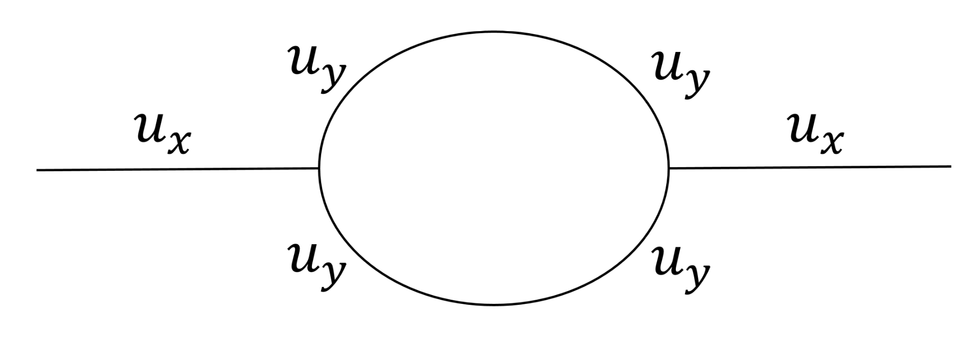
Figure 2: $|$ The one-loop graphical correction to the mass term $u_{x}^{2}$ in the Hamiltonian (41). This arises from the combination of two cubic terms $u_{x}u_{y}^{2}$.

To estimate the length scales beyond which the anharmonic terms become important, we treat the anharmonic terms perturbatively and calculate the corrections to the harmonic terms. These calculations can be illustrated by Feynman diagrams. For example, the correction to the mass term is illustrated in Fig. 2, which leads to the correction to the coefficient $\alpha$:

$$\delta\alpha = \frac{\alpha^{2}}{(2\pi)^{3}v_{0}^{2}}\int{\rm d}^{3}\mathbf{q}{D^{2}\left(2\alpha q_{z}^{2}+gq_{x}^{2}\right)^{2}\over\left[\left(\mu_{x}q_{x}^{2}+\mu_{\rm T}^{0}q_{z}^{2}\right)\left(2\alpha q_{z}^{2}+gq_{x}^{2}\right)+2g\alpha q_{y}^{2}\right]^{2}}$$ (51)

$$= \frac{\alpha^{3/2}D^{2}}{16\sqrt{2}\pi^{2}v_{0}^{2}g^{1/2}}\int{\rm d}q_{x}\int{\rm d}q_{z}{\left(2\alpha q_{z}^{2}+gq_{x}^{2}\right)^{1/2}\over\left(\mu_{x}q_{x}^{2}+\mu_{\rm T}^{0}q_{z}^{2}\right)^{3/2}}\ ,$$ (52)

where we have integrated out $q_{y}$ from $-\infty$ to $\infty$.

The non-linear length $\xi_{x}$ in the $x$-direction is determined by the condition that, for a system of linear extent $\xi_{x}$ in the $x$-direction and infinite in the $y$ and $z$ directions, this correction (51) exactly equals the bare value of $\alpha$. This leads to the condition

$$\alpha=\frac{\alpha^{3/2}D^{2}}{4\sqrt{2}\pi^{2}v_{0}^{2}g^{1/2}}\int_{\xi_{x}^{-1}}^{\infty}{\rm d}q_{x}\int_{0}^{\infty}{\rm d}q_{z}{\left(2\alpha q_{z}^{2}+gq_{x}^{2}\right)^{1/2}\over\left(\mu_{x}q_{x}^{2}+\mu_{\rm T}^{0}q_{z}^{2}\right)^{3/2}}\exp\left[-\left({q_{\perp}\over\Lambda}\right)^{2}\right]\ ,$$ (53)

where we have introduced a smooth ultraviolet cutoff $\Lambda$ through the Gaussian factor $\exp\left[-\left({q_{\perp}\over\Lambda}\right)^{2}\right]$ with $q_{\perp}\equiv\sqrt{q_{x}^{2}+q_{z}^{2}}$, and a factor of $4$ arises from our restriction of the integral to the first quadrant, a restriction that is convenient in the following.

To proceed further we switch to polar coordinates: $q_{x}=q_{\perp}\cos\theta$, $q_{z}=q_{\perp}\sin\theta$; (53) then reduces to

$$1=\frac{\alpha^{1/2}D^{2}}{4\sqrt{2}\pi^{2}v_{0}^{2}g^{1/2}}\int_{0}^{\pi\over 2}{\rm d}\theta{\left(2\alpha\sin^{2}\theta+g\cos^{2}\theta\right)^{1/2}\over\left(\mu_{x}\cos^{2}\theta+\mu_{\rm T}^{0}\sin^{2}\theta\right)^{3/2}}\int_{q_{m}(\theta)}^{\infty}{{\rm d}q_{\perp}\over q_{\perp}}\exp\left[-\left({q_{\perp}\over\Lambda}\right)^{2}\right]\ ,$$ (54)

where we’ve defined

$$q_{m}(\theta)\equiv\xi_{x}^{-1}\sec\theta\ .$$ (55)

It is straightforward to evaluate the integral over $q_{\perp}$ in this expression for $q_{m}\ll\Lambda$, which will always be the case, for all angles $\theta$, when $\Lambda\xi_{x}\gg 1$, as we will verify a posteriori that it is for small noise strength $D$. We find

$$\int_{q_{m}(\theta)}^{\infty}{{\rm d}q_{\perp}\over q_{\perp}}\exp\left[-\left({q_{\perp}\over\Lambda}\right)^{2}\right] =\ln\left({\Lambda\over q_{m}(\theta)}\right)-{C\over 2}+{\cal O}\left[\left({q_{m}\over\Lambda}\right)^{2}\ln\left({q_{m}\over\Lambda}\right)\right]$$ (56)

$$=\ln\left({\Lambda\xi_{x}\cos\theta}\right)-{C\over 2}+{\cal O}\left[\left({1\over\Lambda\xi_{x}\cos\theta}\right)^{2}\ln\left({1\over\Lambda\xi_{x}\cos\theta}\right)\right]\ ,$$

where $C=0.577215664...$ is Euler’s constant.

Dropping the ${\cal O}\left[\left({1\over\Lambda\xi_{x}\cos\theta}\right)^{2}\ln\left({1\over\Lambda\xi_{x}\cos\theta}\right)\right]$ terms, which vanish for $\Lambda\xi_{x}\gg 1$, equation (54) becomes

$$1=\frac{\alpha^{1/2}D^{2}}{4\sqrt{2}\pi^{2}v_{0}^{2}g^{1/2}}\left[A\ln\left({\Lambda^{\prime}\xi_{x}}\right)+G\right]\ ,$$ (57)

where we’ve defined

$$A\equiv\int_{0}^{\pi\over 2}{\rm d}\theta{\left(2\alpha\sin^{2}\theta+g\cos^{2}\theta\right)^{1/2}\over\left(\mu_{x}\cos^{2}\theta+\mu_{\rm T}^{0}\sin^{2}\theta\right)^{3/2}}={1\over\mu_{x}}\sqrt{g\over\mu_{\rm T}^{0}}f(\gamma)$$

$$G\equiv\int_{0}^{\pi\over 2}{\rm d}\theta{\left(2\alpha\sin^{2}\theta+g\cos^{2}\theta\right)^{1/2}\over\left(\mu_{x}\cos^{2}\theta+\mu_{\rm T}^{0}\sin^{2}\theta\right)^{3/2}}\ln\left({\cos\theta}\right)={1\over\mu_{x}}\sqrt{g\over\mu_{\rm T}^{0}}h(\gamma,\Upsilon)\,,$$ (58)

$$f(\gamma)\equiv\left\{\begin{array}[]{ll}\sqrt{\gamma}E(\sqrt{1-\gamma^{-1}})\,\,\,\,\,\,\,\,\,,&\gamma>1\,,\\ \\ E(\sqrt{1-\gamma})\,\,\,\,\,\,\,\,\,\,\,\,\,\,\,\,\,\,,&\gamma<1\,,\end{array}\right.$$ (62)

with $E(k)$ the elliptical integral of the second kind,

$$h(\gamma,\Upsilon)\equiv-{1\over 2}\int_{0}^{\pi\over 2}{\rm d}\phi\cos\phi\sqrt{1+\gamma\tan^{2}\phi}\ln\left(1+\Upsilon\tan^{2}\phi\right)$$ (63)

and

$$\gamma\equiv{2\alpha\mu_{x}\over g\mu_{\rm T}^{0}}\,\ ,\,\,\,\,\Upsilon\equiv{\mu_{x}\over\mu_{\rm T}^{0}}\,\ ,\,\,\,\,\Lambda^{\prime}\equiv\Lambda e^{-C/2}\,\,.$$ (64)

Solving equation(57) for $\xi_{x}$ gives

$$\xi_{x}=\Lambda^{-1}e^{C\over 2}\exp\left[4\sqrt{2}\pi^{2}{v_{0}^{2}\mu_{x}\over D^{2}f(\gamma)}\sqrt{\mu_{\rm T}^{0}\over\alpha}-{h(\gamma,\Upsilon)\over f(\gamma)}\right]\,.$$ (65)

We can now calculate the non-linear length $\xi_{z}$ in the $z$ direction in precisely the same way; that is, by calculating the correction to $\alpha$ in a system of linear extent $\xi_{z}$ in the $z$-direction and infinite in the $x$ and $y$ directions. We now obtain

$$\alpha=\frac{\alpha^{3/2}D^{2}}{4\sqrt{2}\pi^{2}v_{0}^{2}g^{1/2}}\int_{\xi_{z}^{-1}}^{\infty}{\rm d}q_{z}\int_{0}^{\infty}{\rm d}q_{x}{\left(2\alpha q_{z}^{2}+gq_{x}^{2}\right)^{1/2}\over\left(\mu_{x}q_{x}^{2}+\mu_{\rm T}^{0}q_{z}^{2}\right)^{3/2}}\exp\left[-\left({q_{\perp}\over\Lambda}\right)^{2}\right]\ ,$$ (66)

which can again be evaluated by switching to polar coordinates: $q_{x}=q_{\perp}\cos\theta$, $q_{z}=q_{\perp}\sin\theta$; (53), which gives

$$1=\frac{\alpha^{1/2}D^{2}}{4\sqrt{2}\pi^{2}v_{0}^{2}g^{1/2}}\int_{0}^{\pi\over 2}{\rm d}\theta{\left(2\alpha\sin^{2}\theta+g\cos^{2}\theta\right)^{1/2}\over\left(\mu_{x}\cos^{2}\theta+\mu_{\rm T}^{0}\sin^{2}\theta\right)^{3/2}}\int_{q_{mz}(\theta)}^{\infty}{{\rm d}q_{\perp}\over q_{\perp}}\exp\left[-\left({q_{\perp}\over\Lambda}\right)^{2}\right]\ .$$ (67)

The only change from our calculation of $\xi_{x}$ is that the lower cutoff $q_{mz}(\theta)$ is now given by

$$q_{mz}(\theta)\equiv\xi_{z}^{-1}\csc\theta\ .$$ (68)

Proceeding exactly as before, we thereby find that $\xi_{z}$ is determined by the condition:

$$1=\frac{\alpha^{1/2}D^{2}}{4\sqrt{2}\pi^{2}v_{0}^{2}g^{1/2}}\left[A\ln\left({\Lambda^{\prime}\xi_{z}}\right)+G_{2}\right]\ ,$$ (69)

where all symbols are as defined earlier, and

$$G_{2}\equiv\int_{0}^{\pi\over 2}{\rm d}\theta{\left(2\alpha\sin^{2}\theta+g\cos^{2}\theta\right)^{1/2}\over\left(\mu_{x}\cos^{2}\theta+\mu_{\rm T}^{0}\sin^{2}\theta\right)^{3/2}}\ln\left({\sin\theta}\right)\ .$$ (70)

The quickest way to calculate $\xi_{z}$ is simply to subtract equation (69) from equation (57); this gives

$$A\ln\left({\xi_{x}\over\xi_{z}}\right)+G-G_{2}=A\ln\left({\xi_{x}\over\xi_{z}}\right)-\int_{0}^{\pi\over 2}{\rm d}\theta{\left(2\alpha\sin^{2}\theta+g\cos^{2}\theta\right)^{1/2}\over\left(\mu_{x}\cos^{2}\theta+\mu_{\rm T}^{0}\sin^{2}\theta\right)^{3/2}}\ln\left({\tan\theta}\right)=0\ ,$$ (71)

which can obviously be solved for the natural logarithm of the ratio $\xi_{x}/\xi_{z}$:

$$\ln\left({\xi_{x}\over\xi_{z}}\right)={1\over A}\int_{0}^{\pi\over 2}{\rm d}\theta{\left(2\alpha\sin^{2}\theta+g\cos^{2}\theta\right)^{1/2}\over\left(\mu_{x}\cos^{2}\theta+\mu_{\rm T}^{0}\sin^{2}\theta\right)^{3/2}}\ln\left({\tan\theta}\right)\ .$$ (72)

By changing variable of integration from $\theta$ to $u\equiv\tan\theta$, and then changing variables again to $\phi$ defined by $u=\sqrt{\mu_{x}\over\mu_{\rm T}^{0}}\tan\phi$ gives

$$\int_{0}^{\pi\over 2}{\rm d}\theta{\left(2\alpha\sin^{2}\theta+g\cos^{2}\theta\right)^{1/2}\over\left(\mu_{x}\cos^{2}\theta+\mu_{\rm T}^{0}\sin^{2}\theta\right)^{3/2}}\ln\left({\tan\theta}\right)={A\over 2}\ln\left({\mu_{x}\over\mu_{\rm T}^{0}}\right)+{1\over\mu_{x}}\sqrt{g\over\mu_{\rm T}^{0}}\int_{0}^{\pi\over 2}{\rm d}\phi\sqrt{\gamma\sin^{2}\phi+\cos^{2}\phi}\ln\left({\tan\phi}\right)\ .$$ (73)

Using this in (72), and using our earlier result (58) for A, we obtain

$$\ln\left({\xi_{x}\over\xi_{z}}\right)={1\over 2}\ln\left({\mu_{x}\over\mu_{\rm T}^{0}}\right)+{f_{2}(\gamma)\over f(\gamma)}\ ,$$ (74)

where we’ve defined

$$f_{2}(\gamma)\equiv\int_{0}^{\pi\over 2}{\rm d}\phi\sqrt{\gamma\sin^{2}\phi+\cos^{2}\phi}\ln\left({\tan{\phi}}\right)\ .$$ (75)

It is clear by inspection that $f_{2}$ is ${\cal O}(1)$ when $\gamma={\cal O}(1)$. It is also straightforward to show that when $\gamma\gg 1$, $f_{2}(\gamma)\approx\sqrt{\gamma}\ln 2$. Inspection of (62) shows that $f(\gamma)$ is always greater than $1$ , and that $f(\gamma)={\cal O}(1)$ when $\gamma={\cal O}(1)$. In addition, when $\gamma\gg 1$, $f(\gamma)\approx\sqrt{\gamma}$. Putting this all together, we see that, whatever the value of $\gamma$, the ratio ${f_{2}(\gamma)\over f(\gamma)}={\cal O}(1)$. Hence, equation (74) implies

$$\ln\left({\xi_{x}\over\xi_{z}}\right)={1\over 2}\ln\left({\mu_{x}\over\mu_{\rm T}^{0}}\right)+{\cal O}(1)\ ,$$ (76)

which in turn implies

$${\xi_{x}\over\xi_{z}}=\sqrt{\mu_{x}\over\mu_{\rm T}^{0}}\times{\cal O}(1)\ .$$ (77)

This result is, of course, exactly what we would have gotten if we had assumed that the two pieces of the factor $\mu_{x}q_{x}^{2}+\mu_{\rm T}^{0}q_{z}^{2}$ in the propagator are comparable to each other when $q_{x}=\xi_{x}^{-1}$ and $q_{z}=\xi_{z}^{-1}$.

We can now apply the above analysis to a system of finite extent $\xi_{y}$ in the $y$-direction and infinite in the $x$ and $z$-directions. The condition determining $\xi_{y}$ is:

$$1 = \frac{\alpha}{(2\pi)^{3}v_{0}^{2}}\int{\rm d}^{3}\mathbf{q}{D^{2}\left(2\alpha q_{z}^{2}+gq_{x}^{2}\right)^{2}\over\left[\left(\mu_{x}q_{x}^{2}+\mu_{\rm T}^{0}q_{z}^{2}\right)\left(2\alpha q_{z}^{2}+gq_{x}^{2}\right)+2g\alpha q_{y}^{2}\right]^{2}}$$

$$= \frac{\alpha D^{2}}{\pi^{3}v_{0}^{2}}\int_{\xi_{y}^{-1}}^{\infty}{\rm d}q_{y}\int_{0}^{\pi\over 2}{\rm d}\theta\int_{0}^{\infty}{\rm d}q_{\perp}{\left(2\alpha\sin^{2}\theta+g\cos^{2}\theta\right)^{2}q_{\perp}^{5}\over\left[\left(2\alpha\sin^{2}\theta+g\cos^{2}\theta\right)\left(\mu_{x}\cos^{2}\theta+\mu_{\rm T}^{0}\sin^{2}\theta\right)q_{\perp}^{4}+2\alpha gq_{y}^{2}\right]^{2}}\exp\left[-\left({q_{\perp}\over\Lambda}\right)^{2}\right]$$

where we’ve now defined our polar coordinates $q_{\perp}$ and $\theta$ via $q_{x}=q_{\perp}\cos\theta$, $q_{z}=q_{\perp}\sin\theta$.

The integral over $q_{\perp}$ in this expression converges as $q_{\perp}\to\infty$ even without the Gaussian ultraviolet cutoff. This implies that the integral itself will be insensitive to the ultraviolet cutoff $\Lambda$ provided that the $q_{\perp}^{4}$ term in the denominator of (LABEL:syi) dominates the $q_{y}$ term even for $q_{\perp}\sim\Lambda$. Thus we can throw out the Gaussian factor in that integral whenever $2\alpha gq_{y}^{2}\ll\left(2\alpha\sin^{2}\theta+g\cos^{2}\theta\right)\left(\mu_{x}\cos^{2}\theta+\mu_{\rm T}^{0}\sin^{2}\theta\right)\Lambda^{4}$. That is, we can neglect that cutoff for

$$q_{y}\ll\Lambda_{y}(\theta)\equiv\sqrt{\left(2\alpha\sin^{2}\theta+g\cos^{2}\theta\right)\left(\mu_{x}\cos^{2}\theta+\mu_{\rm T}^{0}\sin^{2}\theta\right)\over 2\alpha g}\Lambda^{2}\ .$$ (79)

We’ll show in a moment that, in this regime, the integral over $q_{\perp}$ scales like $q_{y}^{-1}$. On the other hand, for $q_{y}\gg\Lambda_{y}(\theta)$, the $q_{\perp}$ integral converges for $q_{\perp}\sim\Lambda$, at which values of $q_{\perp}$ the denominator of (LABEL:syi) is dominated by the $q_{y}^{2}$ term. In this case, the integral over $q_{\perp}$ scales like $q_{y}^{-4}$. The integral of the latter over $q_{y}$ then converges rapidly as $q_{y}\to\infty$. This implies that $\Lambda_{y}(\theta)$ acts as an effective ultraviolet cutoff on the integral over $q_{y}$. We can therefore approximate (LABEL:syi) by

$$1=\frac{\alpha D^{2}}{\pi^{3}v_{0}^{2}}\int_{0}^{\pi\over 2}{\rm d}\theta\int_{\xi_{y}^{-1}}^{\Lambda_{y}(\theta)}{\rm d}q_{y}\int_{0}^{\infty}{\rm d}q_{\perp}{\left(2\alpha\sin^{2}\theta+g\cos^{2}\theta\right)^{2}q_{\perp}^{5}\over\left[\left(2\alpha\sin^{2}\theta+g\cos^{2}\theta\right)\left(\mu_{x}\cos^{2}\theta+\mu_{\rm T}^{0}\sin^{2}\theta\right)q_{\perp}^{4}+2\alpha gq_{y}^{2}\right]^{2}}\ .$$ (80)

Note that although our argument for the effective ultraviolet cutoff $\Lambda_{y}$ (79) is rather rough, the equation (80) should be quite exact, due to the weakness of the dependence of the integral over $q_{y}$ on that ultraviolet cutoff (that is, the fact that it depends only logarithmically on that cutoff).

The elementary integral over $q_{\perp}$ is

$$\int_{0}^{\infty}{\rm d}q_{\perp}{\left(2\alpha\sin^{2}\theta+g\cos^{2}\theta\right)^{2}q_{\perp}^{5}\over\left[\left(2\alpha\sin^{2}\theta+g\cos^{2}\theta\right)\left(\mu_{x}\cos^{2}\theta+\mu_{\rm T}^{0}\sin^{2}\theta\right)q_{\perp}^{4}+2\alpha gq_{y}^{2}\right]^{2}}={\pi\over 8}{\left(g^{-1}\sin^{2}\theta+(2\alpha)^{-1}\cos^{2}\theta\right)^{1/2}\over\left(\mu_{x}\cos^{2}\theta+\mu_{\rm T}^{0}\sin^{2}\theta\right)^{3/2}q_{y}}\ .$$ (81)

Inserting this into (80) and performing the trivial integral over $q_{y}$ leads to

$$1=\frac{\alpha^{1/2}D^{2}}{8\sqrt{2}\pi^{2}v_{0}^{2}g^{1/2}}\int_{0}^{\pi\over 2}{\rm d}\theta{\left(2\alpha\sin^{2}\theta+g\cos^{2}\theta\right)^{1/2}\over\left(\mu_{x}\cos^{2}\theta+\mu_{\rm T}^{0}\sin^{2}\theta\right)^{3/2}}\ln\left({\Lambda_{y}(\theta)\xi_{y}}\right)\ ,$$ (82)

Using our expression (79) for $\Lambda_{y}(\theta)$ in this expression, we can rewrite it as

$$1=\frac{\alpha^{1/2}D^{2}}{8\sqrt{2}\pi^{2}v_{0}^{2}g^{1/2}}\left[A\ln\left({\Lambda^{2}\xi_{y}}\right)+G_{y}\right]\ ,$$ (83)

where $A$ was defined in (58) and we’ve defined

$$G_{y}\equiv{1\over 2}\int_{0}^{\pi\over 2}{\rm d}\theta{\left(2\alpha\sin^{2}\theta+g\cos^{2}\theta\right)^{1/2}\over\left(\mu_{x}\cos^{2}\theta+\mu_{\rm T}^{0}\sin^{2}\theta\right)^{3/2}}\ln\left[\left(g^{-1}\sin^{2}\theta+(2\alpha)^{-1}\cos^{2}\theta\right)\left(\mu_{x}\cos^{2}\theta+\mu_{\rm T}^{0}\sin^{2}\theta\right)\right]\,.$$ (84)

We can easily use (83) to obtain a simple relation between $\xi_{x}$ and $\xi_{y}$ by taking the ratio of equation (83) to equation (57), which gives

$${\left[A\ln\left({\Lambda^{2}\xi_{y}}\right)+G_{y}\right]\over 2\left[A\ln\left({\Lambda^{\prime}\xi_{x}}\right)+G\right]}=1\ .$$ (85)

This in turn implies

$$A\ln\left({\Lambda^{2}\xi_{y}}\right)+G_{y}=2A\ln\left({\Lambda^{\prime}\xi_{x}}\right)+2G\ .$$ (86)

Gathering the logarithmic terms on one side of this expression, and the constant terms on the other, gives

$$A\ln\left({\Lambda^{2}\xi_{y}\over\left(\Lambda^{\prime}\xi_{x}\right)^{2}}\right)=2G-G_{y}\ ,$$ (87)

which can be solved for $\xi_{y}$:

$$\xi_{y}=\xi_{x}^{2}\exp\left({2G-G_{y}\over A}-C\right)\ ,$$ (88)

where we have used (64) for $\Lambda^{\prime}$. We can further simplify this expression by writing the combination $2G-G_{y}$ as a single integral over $\theta$:

$$2G-G_{y} = \int_{0}^{\pi\over 2}{\rm d}\theta{\left(2\alpha\sin^{2}\theta+g\cos^{2}\theta\right)^{1/2}\over\left(\mu_{x}\cos^{2}\theta+\mu_{\rm T}^{0}\sin^{2}\theta\right)^{3/2}}\left(2\ln(\cos\theta)-{1\over 2}\ln\left[\left({1\over g}\sin^{2}\theta+{1\over 2\alpha}\cos^{2}\theta\right)\left(\mu_{x}\cos^{2}\theta+\mu_{\rm T}^{0}\sin^{2}\theta\right)\right]\right)$$ (89)

$$= -{1\over 2}\int_{0}^{\pi\over 2}{\rm d}\theta{\left(2\alpha\sin^{2}\theta+g\cos^{2}\theta\right)^{1/2}\over\left(\mu_{x}\cos^{2}\theta+\mu_{\rm T}^{0}\sin^{2}\theta\right)^{3/2}}\left(\ln\left[\left({1\over g}\tan^{2}\theta+{1\over 2\alpha}\right)\left(\mu_{x}+\mu_{\rm T}^{0}\tan^{2}\theta\right)\right]\right)\,.$$

Pulling a factor of ${\mu_{x}\over 2\alpha}$ out of the argument of the logarithm in this expression, and using our definition (58) of $A$, we can rewrite this as

$$2G-G_{y}=-{A\over 2}\ln\left({\mu_{x}\over 2\alpha}\right)-{1\over 2}\int_{0}^{\pi\over 2}{\rm d}\theta{\left(2\alpha\sin^{2}\theta+g\cos^{2}\theta\right)^{1/2}\over\left(\mu_{x}\cos^{2}\theta+\mu_{\rm T}^{0}\sin^{2}\theta\right)^{3/2}}\left(\ln\left[\left({2\alpha\over g}\tan^{2}\theta+1\right)\left(1+{\mu_{\rm T}^{0}\over\mu_{x}}\tan^{2}\theta\right)\right]\right)\,.$$ (90)

Now again by changing variable of integration from $\theta$ to $u\equiv\tan\theta$, and then changing variable to $\phi$ defined by $u=\sqrt{\mu_{x}\over\mu_{\rm T}^{0}}\tan\phi$, we obtain, using our definition of $A$ (58) again,

$$2G-G_{y}=-{A\over 2}\left(\ln\left({\mu_{x}\over 2\alpha}\right)+\Psi(\gamma)\right)\,,$$ (91)

where we’ve defined

$$\Psi(\gamma)={1\over f(\gamma)}\int_{0}^{\pi\over 2}{\rm d}\phi\ \ {\cos\phi\sqrt{1+\gamma\tan^{2}\phi}}\ln\left(1+\gamma\tan^{2}\phi\over\cos^{2}\phi\right)\,,$$ (92)

where $f(\gamma)$ was defined in (62), and $\gamma$ was defined in (64). Using the limits (62) on $f(\gamma)$ and this expression (92), it is straightforward to show that the limiting behaviors of $\Psi$ are

$$\Psi(\gamma)=\left\{\begin{array}[]{ll}{\cal O}(1)\,\,\,\,\,\,\,\,\,,&\gamma={\cal O}(1)\,,\\ \\ \ln(\gamma)+{\cal O}(1)\,\,\,\,\,\,\,\,\,\,\,\,\,\,\,\,\,\,,&\gamma\gg 1\,,\end{array}\right.$$ (96)

With the result (91) in hand, we can rewrite (88) as

$$\xi_{y}={\xi_{x}^{2}\over\lambda_{x}}\exp\left(-\frac{1}{2}\Psi(\gamma)+C\right)\ ,$$ (97)

where we’ve defined

$$\lambda_{x}\equiv\sqrt{\mu_{x}\over 2\alpha}\ .$$ (98)

Using the limiting behaviors (96) of $\Psi$ that we just derived, we can obtain the limiting behaviors of $\xi_{y}$:

$$\xi_{y}=\left\{\begin{array}[]{ll}\xi_{y}={\xi_{x}^{2}\over\lambda_{x}}\times{\cal O}(1)\,\,\,\,\,\,\,\,\,,&\gamma={\cal O}(1)\,,\\ \\ {\xi_{x}^{2}\over\lambda_{x}\sqrt{\gamma}}\times{\cal O}(1)\,\,\,\,\,\,\,\,\,\,\,\,\,\,\,\,\,\,,&\gamma\gg 1\,.\end{array}\right.$$ (102)

We can conveniently summarize these two limiting behaviors with a single interpolation formula:

$$\xi_{y}={\xi_{x}^{2}\over\lambda_{x}\sqrt{1+\gamma}}\times{\cal O}(1)\ .$$ (103)

Again this result is exactly what we would have gotten if we had assumed that the two pieces $\left(\mu_{x}q_{x}^{2}+\mu_{\rm T}^{0}q_{z}^{2}\right)\left(2\alpha q_{z}^{2}+gq_{x}^{2}\right)$ and $2g\alpha q_{z}^{2}$ in the denominator in the propagator are comparable to each other when $q_{x}=\xi_{x}^{-1}$, $q_{z}=\xi_{z}^{-1}$, and $q_{y}=\xi_{y}^{-1}$.

Note that all three non-linear lengths diverge exponentially (i.e., like $\exp\left[{{\rm constant}\over D^{2}}\right]$) as the noise strength $D\rightarrow 0$. This strong divergence implies that, in systems with weak noise (small $D$), these three non-linear lengths could become astronomically large. In such systems, the non-linear effects we’ve described in this paper would be undetectable in any realistically sized flock. In this case, our result (50) would hold with the parameters $\alpha$, and $\mu_{x,z}$ simply being constants, rather than the logarithmically diverging or vanishing functions of $q$ that they become for $q$ smaller than $\xi_{x,y,z}$.

In such low noise systems, the logarithms in the real space correlation functions equation (1) of the main text also disappear, leaving only the power law dependences on $x$,$y$, and $z$ given there.

III Calculation of the real-space equal-time correlation functions

Since we have obtained the equal-time correlation function in the momentum space, the equal-time correlation function in real space can be calculated through inverse Fourier transformation:

$$C(\mathbf{r})\equiv\langle\mathbf{u}(\mathbf{r})\cdot\mathbf{u}({\bf 0})\rangle = \int{d^{3}q\over(2\pi)^{3}}\int{d^{3}q^{\prime}\over(2\pi)^{3}}\langle\mathbf{u}(\mathbf{q},t)\cdot\mathbf{u}(\mathbf{q}^{\prime},t)\rangle\exp\left(i\mathbf{q}\cdot\mathbf{r}\right)$$ (104)

$$= \int{d^{3}q\over(2\pi)^{3}}{D\left(gq_{x}^{2}+2\alpha q_{z}^{2}\right)\exp\left(i\mathbf{q}\cdot\mathbf{r}\right)\over\left(\mu_{x}q_{x}^{2}+\mu_{\rm T}^{0}q_{z}^{2}\right)\left(gq_{x}^{2}+2\alpha q_{z}^{2}\right)+2g\alpha q_{y}^{2}}~{}.$$

We will first do this calculation in the linear theory, treating all the coefficients as constants. Once we get the result for the linear theory, we then take these coefficients to be length-dependent so as to take into account anharmonic effects. The length-dependences of these coefficients are inferred from their $q$-dependences, as given by equation (24) of the main text, by replacing $q$ with $1\over r$.

We do the integral over $q_{y}$ first using complex contour techniques. This gives

$$C(\mathbf{r})={D\over 8\pi^{2}\sqrt{2g\alpha}}\int_{-\infty}^{\infty}dq_{x}\int_{-\infty}^{\infty}dq_{z}{\sqrt{2\alpha q_{z}^{2}+gq_{x}^{2}}\exp\left(-\sqrt{2\alpha q_{z}^{2}+gq_{x}^{2}}\sqrt{\mu_{x}q_{x}^{2}+\mu_{\rm T}^{0}q_{z}^{2}\over 2g\alpha}|y|+i\mathbf{q}\cdot\mathbf{r}_{\perp}\right)\over\sqrt{\mu_{x}q_{x}^{2}+\mu_{\rm T}^{0}q_{z}^{2}}}~{},$$ (105)

where $\perp$ denotes $xz$ plane.

Now let’s consider $C(x,y=0,z=0)$:

$$C(x,y=z=0) = {D\over 8\pi^{2}}\int_{-\infty}^{\infty}dq_{x}\exp\left(iq_{x}x-{q_{x}^{2}\over\Lambda^{2}}\right)\int_{-\infty}^{\infty}{dq_{z}\over\sqrt{2g\alpha}}{\sqrt{2\alpha q_{z}^{2}+gq_{x}^{2}}\exp\left(-{q_{z}^{2}\over\Lambda^{2}}\right)\over\sqrt{\mu_{x}q_{x}^{2}+\mu_{\rm T}^{0}q_{z}^{2}}}\,.$$ (106)

Now, define

$$I(q_{x}) \equiv \int_{-\infty}^{\infty}{dq_{z}\over\sqrt{2g\alpha}}{\sqrt{2\alpha q_{z}^{2}+gq_{x}^{2}}\exp\left(-{q_{z}^{2}\over\Lambda^{2}}\right)\over\sqrt{\mu_{x}q_{x}^{2}+\mu_{\rm T}^{0}q_{z}^{2}}}\,,$$ (107)

one can see that this integral converges as $q_{x}\to 0$. Hence, we now write

$$I(q_{x})=I(q_{x}=0)+\delta I(q_{x})\ ,$$ (108)

where $\delta I(q_{x}\to 0)\to 0$ by definition. Putting this into (106), we see immediately that the $I(q_{x}=0)$ piece of this gives rise only to a short-ranged contribution $\propto e^{-(\Lambda x)^{2}}$ to $C(x)$. Hence, all of the long-ranged pieces of $C(x)$ come from $\delta I(q_{x})$. In the following we will first calculate ${\partial I(q_{x})/\partial q_{x}^{2}}$, and then from that result we derive $\delta I(q_{x})$.

Changing the variables of integration in (107) from $q_{z}$ to $Q_{z}$ defined via $q_{z}\equiv\sqrt{\mu_{x}\over\mu_{\rm T}^{0}}Q_{z}$, we get

$${\partial\delta I(q_{x})\over\partial q_{x}^{2}}=\frac{1}{2\mu_{\rm T}^{0}}\sqrt{\frac{\mu_{x}}{g}}\left[\Gamma I_{1}(q_{x})-I_{2}(q_{x})\right]$$ (109)

where

$$I_{1}(q_{x})\equiv\int_{-\infty}^{\infty}dQ_{z}{\exp\left(-{Q_{z}^{2}\over\Lambda_{z}^{2}}\right)\over\sqrt{(q_{x}^{2}+Q_{z}^{2})(\Gamma q_{x}^{2}+Q_{z}^{2})}}\ ,$$ (110)

and

$$I_{2}(q_{x})\equiv\int_{-\infty}^{\infty}dQ_{z}\exp\left(-{Q_{z}^{2}\over\Lambda_{z}^{2}}\right)\sqrt{(\Gamma q_{x}^{2}+Q_{z}^{2})\over(q_{x}^{2}+Q_{z}^{2})^{3}}\ ,$$ (111)

where we’ve defined $\Gamma\equiv{g\mu_{\rm T}^{0}\over 2\alpha\mu_{x}}$ and $\Lambda_{z}\equiv\Lambda\sqrt{\mu_{\rm T}^{0}\over\mu_{x}}$.

We will first calculate $I_{1}$. Since the integral converges rapidly before $Q_{z}$ is comparable to $\Lambda_{z}$, we can ignore the Gaussian cutoff. By a change of variable $Q_{z}=|q_{x}|u$, we have

$$I_{1}\approx\frac{2}{|q_{x}|}\int_{0}^{\infty}\frac{du}{\sqrt{(\Gamma+u^{2})(1+u^{2})}}\ .$$ (112)

The anomalous $q$-dependence of $\alpha$, $\mu_{x}$, and $\mu_{\rm T}$ given by equation (24) of the main text implies that $\Gamma=2g\mu_{\rm T}^{0}/(\alpha\mu_{x})\sim|\ln q|^{1/2}\to\infty$ as $q\rightarrow 0$. We can exploit this fact to split the integral into two easily approximated parts by introducing a constant $B$ such that $1\ll B\ll\sqrt{\Gamma}$:

$$I_{1} \approx \frac{2}{|q_{x}|}\left[\int_{0}^{B}\frac{du}{\sqrt{\Gamma(1+u^{2})}}+\int_{B}^{\infty}\frac{du}{u\sqrt{(\Gamma+u^{2})}}\right]$$ (113)

$$= \frac{2}{\sqrt{\Gamma}|q_{x}|}\left[{\rm arcsinh}(B)+{\rm arcsinh}\left(\frac{\sqrt{\Gamma}}{B}\right)\right]$$ (114)

$$\approx \frac{2}{\sqrt{\Gamma}|q_{x}|}\left[\ln(2B)+\ln\left(\frac{2\sqrt{\Gamma}}{B}\right)\right]$$ (115)

$$= \frac{\ln(16\Gamma)}{\sqrt{\Gamma}|q_{x}|}\ ,$$ (116)

where we have used the fact that $B\gg 1$ and $\sqrt{\Gamma}\gg B$ and used the leading asymptotic expression for the ${\rm arcsinh}$ functions in (115).

We now focus on $I_{2}$, again with the Gaussian cutoff ignored. By the same change of variable $Q_{z}=|q_{x}|u$, we get

$$I_{2}(q_{x}) \approx \frac{2}{|q_{x}|}\int_{0}^{\infty}du\sqrt{\Gamma+u^{2}\over(1+u^{2})^{3}}$$ (117)

$$\approx \frac{2}{|q_{x}|}\left[\int_{0}^{B}du\sqrt{\Gamma\over(1+u^{2})^{3}}+\int_{B}^{\infty}du\frac{\sqrt{\Gamma+u^{2}}}{u^{3}}\right]$$ (118)

$$= \frac{2}{|q_{x}|}\left[\frac{\sqrt{\Gamma}(B+B^{3})}{(1+B^{2})^{3/2}}+\frac{1}{2}\left(\frac{\sqrt{B^{2}+\Gamma}}{B^{2}}+{{\rm arcsinh}(B/\sqrt{\Gamma})\over\sqrt{\Gamma}}\right)\right]$$ (119)

$$\approx \frac{2\sqrt{\Gamma}}{|q_{x}|}$$ (120)

where we have used the fact that $B\gg 1$ in the last approximation.

Substituting the expressions for $I_{1}$ and $I_{2}$ back into (109), we see that, once the wavevector dependences of $\mu_{\rm T}^{0}$, $\mu_{x}$, and $\alpha$ are taken into account, $\Gamma I_{1}\approx{1\over|q_{x}|}\sqrt{\Gamma}\ln\Gamma\gg I_{2}\approx{1\over|q_{x}|}\sqrt{\Gamma}$ as $\mathbf{q}\to 0$, since, as noted earlier, $\Gamma\to\infty$ in that limit. Therefore, the $I_{1}$ term in (109) dominates, so

$${\partial\delta I(q_{x})\over\partial q_{x}^{2}}\approx\frac{1}{2\mu_{\rm T}^{0}}\sqrt{\frac{\mu_{x}\Gamma}{g}}\frac{\ln(16\Gamma)}{|q_{x}|}=\frac{1}{2\sqrt{2\alpha\mu_{\rm T}^{0}}}\frac{\ln(16\Gamma)}{|q_{x}|}\ .$$ (121)

This is easily integrated (keeping in mind that the variable of integration is $q_{x}^{2}$, not $q_{x}$) to obtain

$$\delta I(q_{x})\approx\frac{\ln(16\Gamma)}{\sqrt{2\alpha\mu_{\rm T}^{0}}}|q_{x}|\ .$$ (122)

Substituting this expression back into (106) we get

$$C(x,y=z=0) = {D\ln\left(g\mu_{\rm T}^{0}\over 8\alpha\mu_{x}\right)\over 8\pi^{2}\sqrt{2\alpha\mu_{\rm T}^{0}}}\int_{-\infty}^{\infty}dq_{x}q_{x}\cos\left(q_{x}x\right)\exp\left(-{q_{x}^{2}\over\Lambda^{2}}\right)$$ (123)

$$= {D\ln\left(g\mu_{\rm T}^{0}\over 2\alpha\mu_{x}\right)\over 4\pi^{2}\sqrt{2\alpha\mu_{\rm T}^{0}}}{1\over x^{2}}\int_{0}^{\infty}dQ_{x}Q_{x}\cos Q_{x}\exp\left(-{Q_{x}^{2}\over\Lambda^{2}x^{2}}\right)\,,$$

where in the second equality we have changed variables of integration from $q_{x}$ to $Q_{x}\equiv q_{x}x$. It can be shown that the integral in the last equality of (123) is equal to $-1$ for large $x$ (specifically, for $x\gg 1/\Lambda$). Taking into account the length dependence of the coefficients $\alpha$, $\mu_{x}$, and $\mu_{\rm T}^{0}$ as described at the beginning of this section, we get

$$C(x,y=z=0)\propto-{\left[\ln\left(x\over\xi_{x}\right)\right]^{1\over 4}\ln\left[\ln\left(x\over\xi_{x}\right)\right]\over x^{2}}\,,$$ (124)

where the factor $\xi_{x}^{-1}$ has been added to the arguments of log to make them dimensionless.

Another limit of the correlation function, namely $C(x=y=0,z)$, can be obtained by very similar methods. Starting with:

$$C(x=y=0,z) = {D\over 8\pi^{2}}\int_{-\infty}^{\infty}dq_{z}\exp\left(iq_{z}z-{q_{z}^{2}\over\Lambda^{2}}\right)\int_{-\infty}^{\infty}{dq_{x}\over\sqrt{2g\alpha}}{\sqrt{2\alpha q_{z}^{2}+gq_{x}^{2}}\exp\left(-{q_{z}^{2}\over\Lambda^{2}}\right)\over\sqrt{\mu_{x}q_{x}^{2}+\mu_{\rm T}^{0}q_{z}^{2}}}\,.$$ (125)

We define

$$I_{z}(q_{z}) \equiv \int_{-\infty}^{\infty}{dq_{x}\over\sqrt{2g\alpha}}{\sqrt{2\alpha q_{z}^{2}+gq_{x}^{2}}\exp\left(-{q_{x}^{2}\over\Lambda^{2}}\right)\over\sqrt{\mu_{x}q_{x}^{2}+\mu_{\rm T}^{0}q_{z}^{2}}}\,.$$ (126)

One can see that this integral converges as $q_{x}\to 0$. Hence, we now write

$$I_{z}(q_{x})=I_{z}(q_{x}=0)+\delta I_{z}(q_{x})\ ,$$ (127)

where $\delta I_{z}(q_{z}\to 0)\to 0$ by definition. Putting this into (125), we see immediately that the $I_{z}(q_{z}=0)$ piece of this gives rise only to a short-ranged contribution $\propto e^{-(\Lambda x)^{2}}$ to $C(x=y=0,z)$. Hence, all of the long-ranged pieces of $C(x=y=0,z)$ come from $\delta I_{z}(q_{z})$. In the following we will first calculate ${\partial I_{z}(q_{z})/\partial q_{z}^{2}}$, and then from that result we derive $\delta I_{z}(q_{z})$.

Changing the variables of integration in (126) from $q_{x}$ to $Q_{x}$ defined via $q_{x}\equiv\sqrt{\mu_{\rm T}^{0}\over\mu_{x}}Q_{x}$, we get

$${\partial\delta I_{z}(q_{z})\over\partial q_{z}^{2}}=I_{3}(q_{z})-I_{4}(q_{z})$$ (128)

where

$$I_{3}(q_{z})\equiv{1\over g}\sqrt{\alpha\over 2\mu_{\rm T}^{0}}\int_{-\infty}^{\infty}dQ_{x}{\exp\left(-{Q_{x}^{2}\over\Lambda_{x}^{2}}\right)\over\sqrt{(q_{z}^{2}+Q_{x}^{2})(\Gamma^{-1}q_{z}^{2}+Q_{x}^{2})}}\ ,$$ (129)

and

$$I_{4}(q_{x})\equiv{1\over 2\mu_{x}}\sqrt{\mu_{\rm T}^{0}\over 2\alpha}\int_{-\infty}^{\infty}dQ_{x}\exp\left(-{Q_{x}^{2}\over\Lambda_{x}^{2}}\right)\sqrt{(\Gamma^{-1}q_{z}^{2}+Q_{x}^{2})\over(q_{z}^{2}+Q_{x}^{2})^{3}}\ ,$$ (130)

where we’re using the same definition of $\Gamma$, namely $\Gamma\equiv{g\mu_{\rm T}^{0}\over 2\alpha\mu_{x}}$ and $\Lambda_{x}\equiv\Lambda\sqrt{\mu_{x}\over\mu^{0}_{\rm T}}$.

We will first calculate $I_{3}$. Since the integral converges rapidly before $Q_{x}$ is comparable to $\Lambda_{x}$, we can ignore the Gaussian cutoff. By a change of variable $Q_{x}=|q_{z}|u$, we have

$$I_{3}\approx\frac{1}{|q_{z}|}{1\over g}\sqrt{2\alpha\over\mu_{\rm T}^{0}}\int_{0}^{\infty}\frac{du}{\sqrt{(\Gamma^{-1}+u^{2})(1+u^{2})}}\ .$$ (131)

Since, as noted earlier, $\Gamma=2g\mu_{\rm T}^{0}/\alpha\mu_{x}\sim|\ln q|^{1/2}\to\infty$ as $q\rightarrow 0$, we can split the integral into two parts by introducing a constant $B$ such that $\Gamma^{-1/2}\ll B\ll 1$:

$$I_{3} \approx \frac{2}{|q_{z}|}{1\over g}\sqrt{2\alpha\over\mu_{\rm T}^{0}}\left[\int_{0}^{B}\frac{du}{\sqrt{\Gamma^{-1}+u^{2}}}+\int_{B}^{\infty}\frac{du}{u\sqrt{(1+u^{2})}}\right]$$ (132)

$$= \frac{2}{|q_{z}|}{1\over g}\sqrt{2\alpha\over\mu_{\rm T}^{0}}\left[{\rm arcsinh}(\sqrt{\Gamma}B)+{\rm arcsinh}\left({1\over B}\right)\right]$$ (133)

$$\approx \frac{2}{|q_{z}|}{1\over g}\sqrt{2\alpha\over\mu_{\rm T}^{0}}\left[\ln(2B\sqrt{\Gamma})+\ln\left(\frac{2}{B}\right)\right]$$ (134)

$$= {1\over g}\sqrt{2\alpha\over\mu_{\rm T}^{0}}\frac{\ln(16\Gamma)}{|q_{z}|}\ ,$$ (135)

where we have used the fact that $B\gg 1$ and $\sqrt{\Gamma}\gg B$ and used the leading asymptotic expression for the ${\rm arcsinh}$ functions in (134).

We now turn to $I_{4}$, again with the Gaussian cutoff ignored. By the same change of variable $Q_{x}=|q_{z}|u$, we get

$$I_{4}(q_{z}) \approx {1\over\mu_{x}}\sqrt{\mu_{\rm T}^{0}\over 2\alpha}\frac{1}{|q_{z}|}\int_{0}^{\infty}du\sqrt{\Gamma^{-1}+u^{2}\over(1+u^{2})^{3}}\ .$$ (136)

The integral in this expression is easily seen to approach 1 as $\Gamma\to\infty$. Hence,

$$I_{4}(q_{z}) \approx {1\over\mu_{x}}\sqrt{\mu_{\rm T}^{0}\over 2\alpha}\frac{1}{|q_{z}|}\ .$$ (137)

Comparing the expressions for $I_{3}$ and $I_{4}$, and again using the $q$ dependences of $\alpha$, $\mu_{x}$, and $\mu_{\rm T}^{0}$ from equation (24) of the main text, we find that in $I_{3}$ the prefactor ${1\over g}\sqrt{2\alpha\over\mu_{\rm T}^{0}}\ln\left(16\sqrt{\Gamma}\right)\propto{\ln(|\ln(q)|)\over\sqrt{|\ln(q)|}}\to 0$ as $q\to 0$, while in $I_{4}$ the prefactor ${1\over\mu_{x}}\sqrt{\mu_{\rm T}^{0}\over 2\alpha}$ is independent of $q$. Hence, we can drop $I_{3}$ in (128), and obtain

$${\partial\delta I_{z}(q_{z})\over\partial q_{z}^{2}}\approx-{1\over\mu_{x}}\sqrt{\mu_{\rm T}^{0}\over 2\alpha}\frac{1}{|q_{z}|}\ ,$$ (138)

which can be integrated to give:

$$\delta I_{z}(q_{z})\approx-{1\over\mu_{x}}\sqrt{2\mu_{\rm T}^{0}\over\alpha}|q_{z}|\ .$$ (139)

Substituting this expression back into (125) we get

$$C(x,y=z=0) = -{D\over 4\pi^{2}\mu_{x}}\sqrt{2\mu_{\rm T}^{0}\over\alpha}\int_{0}^{\infty}dq_{z}q_{z}\cos\left(q_{z}z\right)\exp\left(-{q_{z}^{2}\over\Lambda^{2}}\right)$$ (140)

$$= -{D\over 4\pi^{2}\mu_{x}}\sqrt{2\mu_{\rm T}^{0}\over\alpha}{1\over z^{2}}\int_{0}^{\infty}dQ_{z}Q_{z}\cos\left(Q_{z}\right)\exp\left(-{Q_{z}^{2}\over\Lambda^{2}z^{2}}\right)\,,$$

where in the second equality we have changed variables of integration from $q_{z}$ to $Q_{z}\equiv q_{z}z$. The integral in the last equality of (140) is equal to $-1$ for large $z$ (specifically, for $z\gg 1/\Lambda$). Taking into account the length dependence of the coefficients $\mu_{x}$, $\mu_{\rm T}^{0}$, and $\alpha$ as described at the beginning of this section, we find that they cancel out of the prefactor ${1\over\mu_{x}}\sqrt{\mu_{\rm T}^{0}\over\alpha}$. Hence, there are no logs for this direction in real space; instead we find just a simple power law:

$$C(x=y=0,z)\propto-{1\over z^{2}}\,.$$ (141)

Finally let’s turn to $C(x=z=0,y)$. Imposing $x=z=0$ in (105) we obtain

$$C(x=z=0,y)={D\over 8\pi^{2}\sqrt{2g\alpha}}\int_{-\infty}^{\infty}dq_{x}\int_{-\infty}^{\infty}dq_{z}{\sqrt{2\alpha q_{z}^{2}+gq_{x}^{2}}\exp\left(-\sqrt{2\alpha q_{z}^{2}+gq_{x}^{2}}\sqrt{\mu_{x}q_{x}^{2}+\mu_{\rm T}^{0}q_{z}^{2}\over 2g\alpha}|y|\right)\over\sqrt{\mu_{x}q_{x}^{2}+\mu_{\rm T}^{0}q_{z}^{2}}}~{},$$ (142)

where we have dropped the soft cutoff at $\Lambda$ on $q_{\perp}$, since the integral converges at $q_{\perp}\sim 1/\sqrt{y}$, which is much smaller than $\Lambda$ for large $y$. Changing variables from $q_{x,z}$ to $q^{\prime}_{x,z}$ via $q^{\prime}_{x}=\sqrt{\mu_{x}}q_{x}$, $q^{\prime}_{z}=\sqrt{\mu_{\rm T}^{0}}q_{z}$, we get

$$C(x=z=0,y)={D\over 8\pi^{2}\sqrt{2g\alpha\mu_{x}\mu_{\rm T}^{0}}}\int_{-\infty}^{\infty}dq^{\prime}_{x}\int_{-\infty}^{\infty}dq^{\prime}_{z}{\sqrt{{2\alpha{q^{\prime}_{z}}^{2}\over\mu_{\rm T}^{0}}+{g{q^{\prime}_{x}}^{2}\over\mu_{x}}}\exp\left(-\sqrt{{2\alpha{q^{\prime}_{z}}^{2}\over\mu_{\rm T}^{0}}+{g{q^{\prime}_{x}}^{2}\over\mu_{x}}}\sqrt{{q^{\prime}_{\perp}}^{2}\over 2g\alpha}|y|\right)\over q^{\prime}_{\perp}}~{}.$$ (143)

Switching to polar coordinates $q^{\prime}_{x}=q^{\prime}_{\perp}\cos\theta$, $q^{\prime}_{z}=q^{\prime}_{\perp}\sin\theta$, we have

$$C(x=z=0,y) = {D\over 8\pi^{2}\sqrt{2g\alpha\mu_{x}\mu_{\rm T}^{0}}}\int_{0}^{2\pi}d\theta\int_{0}^{\infty}dq_{\perp}\ \ {q^{\prime}_{\perp}\sqrt{{2\alpha\sin^{2}\theta\over\mu_{\rm T}^{0}}+{g\cos^{2}\theta\over\mu_{x}}}}$$ (144)

$$\times\exp\left(-\sqrt{{2\alpha\sin^{2}\theta\over\mu_{\rm T}^{0}}+{g\cos^{2}\theta\over\mu_{x}}}\sqrt{1\over 2g\alpha}{q^{\prime}_{\perp}}^{2}|y|\right)$$

$$= {D\over 8\pi\sqrt{\mu_{x}\mu_{\rm T}^{0}}}{1\over|y|}~{}.$$

Taking into account the length-dependences of the coefficients we get

$$C(x=z=0,y)\sim{\left[\ln\left(|y|\over\xi_{y}\right)\right]^{-{3\over 8}}\over|y|}\,.$$ (145)

References

• (1) S. Ramaswamy, The mechanics and statics of active matter. Ann. Rev. Condens. Matt. Phys. 1, 323-345 (2010); M.C. Marchetti, J.F. Joanny, S. Ramaswamy, T.B. Liverpool, J. Prost, M. Rao, and R.A. Simha, Hydrodynamics of soft active matter, Rev. Mod. Phys. 85, 1143-1188 (2013); C. Bechinger, R. Di Leonardo, H. L${\rm\ddot{o}}$wen, C. Reichhardt, G. Volpe, and G. Volpe, Active particles in complex and crowded environments, Rev. Mod. Phys. 88, 045006 (2016); F. Schweitzer, Brownian Agents and Active Particles: Collective Dynamics in the Natural and Social Sciences, Springer Series in Synergetics (Springer, New York, 2003).
• (2) L. Golubović and M. Golubović, Fluctuations of Quasi-Two-Dimensional Smectics Intercalated between Membranes in Multilamellar Phases of DNA-Cationic Lipid Complexes. Phys. Rev. Lett. 80, 4341 (1998).
• (3) C.H. O’Hern, and T.C. Lubensky, Sliding Columnar Phase of DNA-Lipid Complexes. Phys. Rev. Lett. 80, 4345 (1998).
• (4) C.H. O’Hern, and T.C. Lubensky, Nonlinear elasticity of the sliding columnar phase. Phys. Rev. E 58, 5948 (1998).
• (5) J.R. Howse, R.A.L. Jones, A.J. Ryan, T. Gough, R. Vafabakhsh, and R. Golestanian, Self-motile colloidal particles: From directed propulsion to random walk. Phys. Rev. Lett. 99, 048102 (2007).
• (6) A. Bricard, J.-B. Caussin, N. Desreumaux, O. Dauchot, and D. Bartolo, Emergence of macroscopic directed motion in populations of motile colloids. Nature 503, 95-104 (2013).
• (7) J. Toner, and Y.-h. Tu, Long-range order in a two-dimensional dynamical XY model: how birds fly together. Phys. Rev. Lett. 75, 4326 (1995).
• (8) J. Toner, and Y.-h. Tu, Flocks, herds, and schools: a quantitative theory of flocking. Phys. Rev. E 58, 4828(1998).
• (9) J. Toner, Y.-h. Tu, and S. Ramaswamy, Hydrodynamics and phases of flocks. Ann. Phys. 318, 170(2005).
• (10) J. Toner, A Reanalysis of the hydrodynamic theory of fluid, polar-ordered flocks. Phys. Rev. E 86, 031918 (2012).
• (11) D. Forster, D.R. Nelson, and M.J. Stephen, Large-distance and long-time properties of a randomly stirred fluid. Phys. Rev. A 16, 732 (1977).
• (12) Supplemental material.
• (13) L. Chen, J. Toner, and C.F. Lee, Critical phenomenon of the order-disorder transition in incompressible active fluids. New J. Physics 17, 042002 (2015).
• (14) L. Chen, C.F. Lee, and J. Toner, Mapping two-dimensional polar active fluids to two-dimensional soap and one-dimensional sandblasting. Nat. Commun. 7, 12215 (2016).
• (15) G. Grinstein, and R.A. Pelcovits, Anharmonic effects in bulk smectic liquid crystals and other “one-dimensional solids”. Phys. Rev. Lett. 47, 856 (1981).
• (16) C. Battle, C.P. Broedersz, N. Fakhri, V.F. Geyer, J. Howard, C.F. Schmidt, and F.C. MacKintosh, Broken detailed balance at mesoscopic scales in active biological systems. Science 352 604 (2016).
• (17) C. Nardini, E. Fodor, E. Tjhung, F. van Wijland, J. Tailleur, and M.E. Cates, Entropy production in field theories without time reversal symmetry: Quantifying the non-equilibrium character of active matter. Physical Review X 7, 021007 (2017).
• (18) The elastic energy of the system must be invariant with respect to uniform, rigid rotations about the $z$-axis. Hence strictly speaking, to meet this symmetry requirement the exact expression for the first piece in (25) should be ${B\over 2}\left[\partial_{y}h-{(\partial_{x}h)^{2}\over 2}-{(\partial_{y}h)^{2}\over 2}\right]^{2}$. However, the newly added $-(\partial_{y}h)^{2}/2$ in the parenthesis only introduces anharmonic terms which are irrelevant in the long wavelength limit.
Supplemental Materials: