Primal-Dual Distributed Temporal Difference Learning

Abstract

The goal of this paper is to study a distributed temporal-difference (TD)-learning algorithm for a class of multi-agent Markov decision processes (MDPs). The single-agent TD-learning is a reinforcement learning (RL) algorithm to evaluate an accumulated rewards corresponding to a given policy. In multi-agent settings, multiple RL agents concurrently behave following its own local behavior policy and learn the accumulated global rewards, which is a sum of the local rewards. The goal of each agent is to evaluate the accumulated global rewards by only receiving its local rewards. The algorithm shares learning parameters through random network communications, which have a randomly changing undirected graph structures. The problem is converted into a distributed optimization problem and the corresponding saddle-point problem of its Lagrangian function. The propose TD-learning is a stochastic primal-dual algorithm to solve it. We prove finite-time convergence of the algorithm with its convergence rates and sample complexity.

, ,

1 Introduction

We develop a new multi-agent temporal-difference (TD)-learning algorithm, called a distributed gradient temporal-difference (DGTD) learning, for multi-agent Markov decision processes (MDPs). TD-learning [1, 2] is a reinforcement learning (RL) algorithm to learn an accumulated discounted rewards for a given policy without the model knowledge, which is called the policy evaluation problem. In our multi-agent RL setting, $N$ RL agents concurrently behave and learn the accumulated global rewards, which is a sum of the local rewards, where each agent $i$ only receives local reward following its own local behavior policy $\pi_{i}$. The main challenge is the information limitation: each agent is only accessible to its local reward which only contains partial information on the global reward. The algorithm assumes additional partial information sharing among agents, e.g., sharing of learning parameters, through random network communications, where the network structure is represented by a randomly changing undirected graph. Despite the additional communication model, the algorithm is still distributed in the sense that each agent has a local view of the overall system: it is only accessible to the learning parameter of the neighboring RL agents in the graph. Potential applications are distributed machine learning, distributed resource allocation, and robotics, where the reward information is limited due to physical limitations (spacial limits in robotics or infrastructure limits in resource allocation) or privacy constraints.

The proposed DGTD generalizes the single-agent GTD [1, 2] to the multi-agent MDPs. The algorithm is derived according to the following steps: we cast the multi-agent policy evaluation problem as the distributed optimization problem

$$\min_{w^{(i)}}\sum_{i=1}^{N}{f_{i}(w^{(i)})}\quad{\rm subject\,\,to}\quad w^{(1)}=w^{(2)}=\cdots=w^{(N)},$$ (1)

where $f_{i}$ is an objective of each agent, related to the Bellman loss function, and a corresponding single saddle-point optimization problem. The averaging consensus-based algorithms [3] are popular for solving the distributed optimization (1). Different from the averaging consensus-based algorithms, the proposed DGTD applies the primal-dual saddle-point approach [4, 5, 6, 7, 8, 9] to multi-agent RLs, where primal-dual algorithms are developed for the distributed optimization. Their main idea is to convert the constraints $w^{(1)}=w^{(2)}=\cdots=w^{(N)}$ in (1) into a single equality constraint with the graph Laplacian matrix, and solve the optimization by using the Lagrangian duality. It is known that they provide effective convergence rates with constant step-sizes for deterministic problems. We generalize it to stochastic cases using the stochastic primal-dual method [10], and apply to the policy evaluation problem. Advantages of the primal-dual approach is that analysis tools from optimization perspectives, such as [11, 12, 10, 4, 5, 6] can be easily applied to prove its convergence, and the case of random communication networks can be easily addressed.

The main contributions are summarized as follows:

1. To the author’s knowledge, the proposed DGTD is the first multi-agent off-policy RL algorithm which guarantees convergence under distributed rewards. Only recently, [13] and [14] suggest multi-agent off-policy RLs at or after the time of initial submission of this paper. The differences are summarized shortly later.

2. This study provides a general and unified saddle-point framework of the distributed policy evaluation problem, which offers more algorithmic flexibility such as additional cost constraints and objective, for example, entropic measures and sparsity promoting objectives. In particular, we formalize the distributed policy evaluation problem as a distributed optimization, and then convert it into a single saddle-point problem. Another advantage of this approach is that it easily addresses the case of random communication networks.

3. Rigorous analysis is given for the policy evaluation problem and the DGTD. In particular, we provide analysis of solutions of the proposed saddle-point problem including bounds on the solutions, and prove that the policy evaluation problem can be solved by addressing the saddle-point problem. We also provide rigorous convergence rates and sample complexity of the proposed algorithm, which are currently laking in the literature.

Related works: Recently, some progresses have been made in multi-agent RLs [15, 16, 17, 18, 19]. For the policy optimization problem, the distributed Q-learning (QD-learning) [15], distributed actor-critic algorithm [16, 20], and distributed fitted Q-learning [21] are studied in multi-agent settings. The work in [22] considers an approximation distributed Q-learning with neural nonlinear function approximation. For the policy evaluation problem, distributed GTD algorithms are studied in [17, 18, 23, 13, 24, 14, 24]. The results in [17, 18, 24] consider central rewards with different assumptions. The result in [23] suggests a distributed TD learning with an averaging consensus steps, and proves its convergence rate. The main difference is that [23] considers an on-policy learning, while this work considers off-policy learning methods. The TD learning in [13] considers a stochastic primal-dual algorithm for the policy evaluation with stochastic variants of the consensus-based distributed subgradient method akin to [25]. The main difference is that the algorithm in [13] introduces gradient surrogates of the objective function with respect to the local primal and dual variables, and the mixing steps for consensus are applied to both the local parameters and local gradient surrogates. However, rigorous convergence analysis, such as the sample complexity and convergence with high probability, is lacking in [13] compared to the work in this paper. The work in [14] develops the so-called homotopy stochastic primal-dual algorithm with ${\mathcal{O}}(1/T)$ rate for strongly convex strongly concave min-max problems, where $T$ is the total number of iterations. The rate is faster than the rate of the proposed algorithm, ${\mathcal{O}}(1/\sqrt{T})$. However, the new algorithm can be applied to the proposed formulation and improve our result. Moreover, rigorous analysis of solutions is lacking in [14].

Preliminary results are included in the conference version [26], which only provides asymptotic convergence based on the stochastic approximation method [27] and control theory. However, the convergence without its rates and complexity analysis does not guarantee efficiency of the algorithm, which is essential in contemporary optimization and learning algorithms. The convergence rate analysis is usually more challenging and requires substantially more works. In this paper, we provide more rigorous and comprehensive analysis of solutions and finite-time convergence rate analysis with sample complexities based on results in convex optimization, which is not possible in the control theoretic approach in [26]. Besides, we consider stochastic network communications and a modified algorithm to improve its convergence properties.

2 Preliminaries

2.1 Notation and terminology

The following notation is adopted: ${\mathbb{R}}^{n}$ denotes the $n$-dimensional Euclidean space; ${\mathbb{R}}^{n\times m}$ denotes the set of all $n\times m$ real matrices; ${\mathbb{R}}_{+}$ and ${\mathbb{R}}_{++}$ denote the sets of nonnegative and positive real numbers, respectively, $A^{T}$ denotes the transpose of matrix $A$; $I_{n}$ denotes the $n\times n$ identity matrix; $I$ denotes the identity matrix with appropriate dimension; $\|\cdot\|_{2}$ denotes the standard Euclidean norm; $\|x\|_{D}:=\sqrt{x^{T}Dx}$ for any positive-definite $D$; $\lambda_{\min}(A)$ denotes the minimum eigenvalue of $A$ for any symmetric matrix $A$; $|{\mathcal{S}}|$ denotes the cardinality of the set for any finite set ${\mathcal{S}}$; ${\mathbb{E}}[\cdot]$ denotes the expectation operator; ${\mathbb{P}}[\cdot]$ denotes the probability of an event; $[x]_{i}$ is the $i$-th element for any vector $x$; $[P]_{ij}$ indicates the element in $i$-th row and $j$-th column for any matrix $P$; if ${\bf z}$ is a discrete random variable which has $n$ values and $\mu\in{\mathbb{R}}^{n}$ is a stochastic vector, then ${\bf z}\sim\mu$ stands for ${\mathbb{P}}[{\bf z}=i]=[\mu]_{i}$ for all $i\in\{1,\ldots,n\}$; ${\bf 1}_{n}\in{\mathbb{R}}^{n}$ denotes an $n$-dimensional vector with all entries equal to one; ${\rm dist}({\mathcal{S}},x)$ denotes the standard Euclidean distance of a vector $x$ from a set ${\mathcal{S}}$, i.e., ${\rm dist}({\mathcal{S}},x):=\inf_{y\in{\mathcal{S}}}\|x-y\|_{2}$; for any ${\mathcal{S}}\subset{\mathbb{R}}^{n}$, ${\rm diam}({\mathcal{S}}):=\sup_{x\in{\mathcal{S}},y\in{\mathcal{S}}}\|x-y\|_{2}$ is the diameter of the set $\mathcal{S}$; for a convex closed set $\mathcal{S}$, $\Gamma_{\mathcal{S}}(x)$ is the projection of $x$ onto the set $\mathcal{S}$, i.e., $\Gamma_{\mathcal{S}}(x):=\operatorname{arg\,min}_{y\in{\mathcal{S}}}\|x-y\|_{2}$; a continuously differentiable function $f:{\mathbb{R}}^{n}\to{\mathbb{R}}$ is convex if $f(y)\geq f(x)+(y-x)^{T}\nabla f(x),\forall x,y\in{\mathbb{R}}^{n}$ and $\rho$-strongly convex if $f(y)\geq f(x)+(y-x)^{T}\nabla f(x)+(\rho/2)\|x-y\|^{2},\forall x,y\in{\mathbb{R}}^{n}$ [28, pp. 691]; $f_{x}(\bar{x})$ is a subgradient of a convex function $f:{\mathbb{R}}^{n}\to{\mathbb{R}}$ at a given vector $\bar{x}\in{\mathbb{R}}^{n}$ when the following relation holds: $f(\bar{x})+f_{x}(\bar{x})^{T}(x-\bar{x})\leq f(x)$for all $x\in{\mathbb{R}}^{n}$ [12, pp. 209].

2.2 Graph theory

An undirected graph with the node set ${\mathcal{V}}$ and the edge set ${\mathcal{E}}\subseteq{\mathcal{V}}\times{\mathcal{V}}$ is denoted by ${\mathcal{G}}=({\mathcal{E}},{\mathcal{V}})$. We define the neighbor set of node $i$ as ${\mathcal{N}}_{i}:=\{j\in{\mathcal{V}}:(i,j)\in{\mathcal{E}}\}$. The adjacency matrix of $\mathcal{G}$ is defined as a matrix $W$ with $[W]_{ij}=1$, if and only if $(i,j)\in{\mathcal{E}}$. If $\mathcal{G}$ is undirected, then $W=W^{T}$. A graph is connected, if there is a path between any pair of vertices. The graph Laplacian is $L=H-W$, where $H$ is a diagonal matrix with $[H]_{ii}=|{\mathcal{N}}_{i}|$. If the graph is undirected, then $L$ is symmetric positive semi-definite. It holds that $L{\bf 1}_{|{\mathcal{V}}|}=0$. If ${\mathcal{G}}$ is connected, $0$ is a simple eigenvalue of $L$, i.e., ${\bf 1}_{|{\mathcal{V}}|}$ is the unique eigenvector corresponding to $0$, and the span of ${\bf 1}_{|{\mathcal{V}}|}$ is the null space of $L$.

2.3 Random communication network

We will consider a random communication network model considered in [29]. In this paper, agents communicate with neighboring agents and update their estimates at discrete time instances $k\in\{0,1,\ldots\}$ over random time-varying network ${\mathcal{G}}(k):=({\mathcal{E}}(k),{\mathcal{V}}(k)),k\in\{1,2,\ldots\}$. Let ${\mathcal{N}}_{i}(k):=\{j\in{\mathcal{V}}(k):(i,j)\in{\mathcal{E}}(k)\}$ be the neighbor set of agent $i$, $W(k)$ be the adjacency matrix of ${\mathcal{G}}(k)$, and $H(k)$ be a diagonal matrix with $[H(k)]_{ii}=|{\mathcal{N}}_{i}(k)|$. Then, the graph Laplacian of ${\mathcal{G}}(k)$ is $L(k):=H(k)-W(k)$. We assume that ${\mathcal{G}}(k)$ is a random graph that is independent and identically distributed over time $k$. A formal definition of the random graph is given below.

Assumption 1.

Let ${\mathcal{F}}:=(\Omega,{\mathcal{B}},\mu)$ be a probability space such that $\Omega$ is the set of all $|{\mathcal{V}}|\times|{\mathcal{V}}|$ adjacency matrices, ${\mathcal{B}}$ is the Borel $\sigma$-algebra on $\Omega$ and $\mu$ is a probability measure on ${\mathcal{B}}$. We assume that for all $k\geq 0$, the matrix $W(k)$ is drawn from probability space ${\mathcal{F}}$.

Define the expected value of the random matrices $W(k),H(k),L(k)$, respectively, by

$${\bf W}:={\mathbb{E}}[W(k)],\quad{\bf H}:={\mathbb{E}}[H(k)],$$

$${\bf L}:={\mathbb{E}}[L(k)]={\bf H}-{\bf W},$$

for all $k\geq 0$. An edge set induced by the positive elements of the matrix ${\bf W}$ is ${\bf E}:=\{(j,i)\in{\mathcal{V}}\times{\mathcal{V}}:[{\bf{W}}]_{ij}>0\}$. Consider the corresponding graph $({\bf E},{\mathcal{V}})$, which we refer to as the mean connectivity graph [29]. We consider the following connectivity assumption for the graph.

Assumption 2 (Mean connectivity).

The mean connectivity graph $({\bf E},{\mathcal{V}})$ is connected.

Under 2, $0$ is a simple eigenvalue of ${\bf L}$ [30, Lemma 1]. It implies that ${\bf L}{\bf 1}_{|{\mathcal{V}}|}=0$ holds, and later this assumption is used for the consensus of learning parameters.

2.4 Reinforcement learning overview

We briefly review a basic single-agent RL algorithm from [31] with linear function approximation. A Markov decision process (MDP) is characterized by a quadruple ${\mathcal{M}}:=({\mathcal{S}},{\mathcal{A}},P,r,\gamma)$, where ${\mathcal{S}}$ is a finite state space (observations in general), $\mathcal{A}$ is a finite action space, $P(s,a,s^{\prime}):={\mathbb{P}}[s^{\prime}|s,a]$ represents the (unknown) state transition probability from state $s$ to $s^{\prime}$ given action $a$, $\hat{r}:{\mathcal{S}}\times{\mathcal{A}}\times{\mathcal{S}}\to[0,\sigma]$, where $\sigma>0$ is the bounded random reward function, and $\gamma\in(0,1)$ is the discount factor. If action $a$ is selected with the current state $s$, then the state transits to $s^{\prime}$ with probability $P(s,a,s^{\prime})$ and incurs a random reward $\hat{r}(s,a,s^{\prime})\in[0,\sigma]$ with expectation $r(s,a,s^{\prime})$. The stochastic policy is a map $\pi:{\mathcal{S}}\times{\mathcal{A}}\to[0,1]$ representing the probability $\pi(s,a)={\mathbb{P}}[a|s]$, $P^{\pi}$ denotes the transition matrix whose $(s,s^{\prime})$ entry is ${\mathbb{P}}[s^{\prime}|s]=\sum_{a\in{\mathcal{A}}}{P(s,a,s^{\prime})\pi(s,a)}$, and $d:{\mathcal{S}}\to{\mathbb{R}}$ denotes the stationary distribution of the state $s\in{\mathcal{S}}$ under the behavior policy $\beta$. We also define $r^{\pi}(s)$ as the expected reward given the policy $\pi$ and the current state $s$, i.e.

$$r^{\pi}(s) :=\sum_{a\in{\mathcal{A}}}{\sum_{s^{\prime}\in{\mathcal{S}}}{\pi(s,a)P(s,a,s^{\prime})r(s,a,s^{\prime})}}.$$

The infinite-horizon discounted value function with policy $\pi$ and reward $\hat{r}$ is

$$J^{\pi}(s):={\mathbb{E}}\left[\left.\sum_{k=0}^{\infty}{\gamma^{k}\hat{r}(s_{k},a_{k},s_{k+1})}\right|s_{0}=s\right],$$

where ${\mathbb{E}}$ stands for the expectation taken with respect to the state-action trajectories following the state transition $P^{\pi}$. Given pre-selected basis (or feature) functions $\phi_{1},\ldots,\phi_{q}:{\mathcal{S}}\to{\mathbb{R}}$, $\Phi\in{\mathbb{R}}^{|{\mathcal{S}}|\times q}$ is defined as a full column rank matrix whose $s$-th row vector is $\phi(s):=\begin{bmatrix}\phi_{1}(s)&\cdots&\phi_{q}(s)\end{bmatrix}$. The goal of RL with the linear function approximation is to find the weight vector $w$ such that $J_{w}:=\Phi w$ approximates the true value function $J^{\pi}$. This is typically done by minimizing the mean-square Bellman error loss function [2]

$$\min_{w\in{\mathbb{R}}^{q}}{\rm MSBE}(w):=\frac{1}{2}\|r^{\pi}+\gamma P^{\pi}\Phi w-\Phi w\|_{D}^{2},$$ (2)

where $D$ is a symmetric positive-definite matrix and $r^{\pi}\in{\mathbb{R}}^{|{\mathcal{S}}|}$ is a vector enumerating all $r^{\pi}(s),s\in{\mathcal{S}}$. For online learning, we assume that $D$ is a diagonal matrix with positive diagonal elements $d(s),s\in{\mathcal{S}}$. In the model-free learning, a stochastic gradient descent method can be applied with a stochastic estimates of the gradient $\nabla_{w}{\rm MSBE}(w)=(\gamma P^{\pi}\Phi-\Phi)^{T}D(r^{\pi}+\gamma P^{\pi}\Phi w-\Phi w)$. The temporal difference (TD) learning [31, 32] with a linear function approximation is a stochastic gradient descent method with stochastic estimates of the approximate gradient $\nabla_{w}{\rm MSBE}(w)\cong(-\Phi)^{T}D(r^{\pi}+\gamma P^{\pi}\Phi w-\Phi w)$, which is obtained by dropping $\gamma P^{\pi}\Phi$ in $\nabla_{w}{\rm MSBE}(w)$. If the linear function approximation is used, then this algorithm converges to an optimal solution of (2). The GTD in [2] solves instead the minimization of the mean-square projected Bellman error loss function

$$\min_{w\in{\mathbb{R}}^{q}}{\rm MSPBE}(w):=\frac{1}{2}\|\Pi(r^{\pi}+\gamma P^{\pi}\Phi w)-\Phi w\|_{D}^{2},$$ (3)

where $\Pi$ is the projection onto the range space of $\Phi$, denoted by $R(\Phi)$: $\Pi(x):=\operatorname{arg\,min}_{x^{\prime}\in R(\Phi)}\|x-x^{\prime}\|_{D}^{2}$. The projection can be performed by the matrix multiplication: we write $\Pi(x):=\Pi x$, where $\Pi:=\Phi(\Phi^{T}D\Phi)^{-1}\Phi^{T}D$. Compared to the standard TD learning, the main advantage of the GTD algorithms [1, 2] is their off-policy learning abilities.

Remark 1.

Although its direct application to real problems is limited, the policy evaluation problem is a fundamental problem which is a critical building block to develop more practical policy optimization algorithms such as SALSA [33] and actor-critic [34] algorithms.

Note that $d$ depends on the behavior policy, $\beta$, while $P^{\pi}$ and $r^{\pi}$ depend on the target policy, $\pi$, that we want to evaluate. This corresponds to the off-policy learning. The main problem is to obtain samples, $(s,a,\hat{r},s^{\prime})$ under $\pi$, from the samples under $\beta$. It can be done by the importance sampling or sub-sampling techniques [1]. Throughout the paper, we mostly consider the case $\beta=\pi$ (on-policy) for simplicity. However, it can be generalized to the off-policy learning with simple modifications.

3 Distributed reinforcement learning overview

In this section, we introduce the notion of the distributed RL, which will be studied throughout the paper. Consider $N$ RL agents labelled by $i\in\{1,\ldots,N\}=:{\mathcal{V}}$. A multi-agent Markov decision process is characterized by $({\mathcal{S}},\{{\mathcal{A}}_{i}\}_{i\in{\mathcal{V}}},P,\{\hat{r}_{i}\}_{i\in{\mathcal{V}}},\gamma)$, where $\gamma\in(0,1)$ is the discount factor, ${\mathcal{S}}$ is a finite state space, ${\mathcal{A}}_{i}$ is a finite action space of agent $i$, $a:=(a_{1},\ldots,a_{N})$ is the joint action, ${\mathcal{A}}:=\prod_{i=1}^{N}{{\mathcal{A}}_{i}}$ is the corresponding joint action space, $\hat{r}_{i}:{\mathcal{S}}\times{\mathcal{A}}\times{\mathcal{S}}\to[0,\sigma]$, $\sigma>0$, is a bounded random reward of agent $i$ with expectation $r_{i}(s,a,s^{\prime})$, and $P(s,a,s^{\prime}):={\mathbb{P}}[s^{\prime}|s,a]$ represents the transition model of the state $s$ with the joint action $a$ and the corresponding joint action space ${\mathcal{A}}$. The stochastic policy of agent $i$ is a mapping $\pi_{i}:{\mathcal{S}}\times{\mathcal{A}}_{i}\to[0,1]$ representing the probability $\pi_{i}(s,a_{i})={\mathbb{P}}[a_{i}|s]$ and the corresponding joint policy is $\pi(s,a):=\prod_{i=1}^{N}{\pi_{i}(s,a_{i})}$. $P^{\pi}$ denotes the transition matrix, whose $(s,s^{\prime})$ entry is ${\mathbb{P}}[s^{\prime}|s]=\sum_{a\in{\mathcal{A}}}{P(s,a,s^{\prime})\pi(s,a)}$, $d:{\mathcal{S}}\to{\mathbb{R}}$ denotes the stationary state distribution under the policy $\pi$. In particular, if the joint action $a$ is selected with the current state $s$, then the state transits to $s^{\prime}$ with probability $P(s,a,s^{\prime})$, and each agent $i$ observes a random reward $\hat{r}_{i}(s,a,s^{\prime})\in[0,\sigma]$ with expectation $r_{i}(s,a,s^{\prime})$. We assume that each agent does not have access to other agents’ rewards. For instance, there exists no centralized coordinator; thereby each agent does not know other agents’ rewards. In another example, each agent/coordinator may not want to uncover his/her own goal or the global goal for security/privacy reasons. We denote by $r_{i}^{\pi}(s)$ the expected reward of agent $i$, given the current state $s$

$$r_{i}^{\pi}(s):=\sum_{a\in A}{\sum_{s^{\prime}\in{\mathcal{S}}}{\pi(s,a)P(s,a,s^{\prime})r_{i}(s,a,s^{\prime})}}.$$

Throughout the paper, a vector enumerating all $r_{i}^{\pi}(s),s\in{\mathcal{S}}$ is denoted by $r_{i}^{\pi}\in{\mathbb{R}}^{|{\mathcal{S}}|}$. In addition, denote by $P_{i}(s,a,s_{i}^{\prime})$ the state transition probability of agent $i$ given joint state $s$ and joint action $a$. We can consider one of the following two scenarios throughout the paper.

1. All agents can observe the identical state $s$. For example, transitions of multiple ground robots avoiding collisions with each other may depend on other robots actions and states, while they needs to know the global state, e.g., locations of all robots.

2. All agents observe different states, while each agent’s state transition is independent of the other agents’ states and actions, i.e., they are fully decoupled. For example, each agent observes its own state which is sampled independently from the state transition probability of the MDP. For another instance, multiple robots navigating separated regions do not affect other agents’ transitions.

In this paper, we assume that the MDP with given $\pi$ has a stationary distribution.

Assumption 3.

With a fixed policy $\pi$, the Markov chain $P^{\pi}$ is ergodic with the stationary distribution $d$ with $d(s)>0,s\in{\mathcal{S}}$.

In addition, we summarize definitions and notations for some important quantities below.

1. $D$ is defined as a diagonal matrix with diagonal entries equal to those of $d$.

2. $J^{\pi}$ is the infinite-horizon discounted value function with policy $\pi$ and reward $\hat{r}=(\hat{r}_{1}+\cdots+\hat{r}_{N})/N$ defined as $J^{\pi}$ satisfying $J^{\pi}=\frac{1}{N}\sum_{i=1}^{N}{r_{i}^{\pi}}+\gamma P^{\pi}J^{\pi}$.

3. We denote $\xi:=\min_{s\in{\mathcal{S}}}d(s)$.

The goal is to learn an approximate value of the centralized reward $\hat{r}=(\hat{r}_{1}+\cdots+\hat{r}_{N})/N$ as stated below.

Problem 1 (Multi-agent RL problem (MARLP)).

In the multi-agent RL problem, the goal of each agent $i$ is to learn an approximate value function of the centralized reward $\hat{r}=(\hat{r}_{1}+\cdots+\hat{r}_{N})/N$.

Our first step to develop a decentralized RL algorithm to solve 1 is to convert the problem into an equivalent optimization problem. In particular, we can prove that solving 1 is equivalent to solving the optimization problem

$$\min_{w\in C}\sum_{i=1}^{N}{{\rm MSPBE}_{i}(w)},$$ (4)

where ${\rm MSPBE}_{i}$ is defined as ${\rm MSPBE}_{i}(w):=\frac{1}{2}\|\Pi(r_{i}^{\pi}+\gamma P^{\pi}\Phi w)-\Phi w\|_{D}^{2}$ for all $i\in\{1,2,\ldots,N\}$, $C\subset{\mathbb{R}}^{q}$ is assumed to be a compact convex set which includes an unconstrained global minimum of (4).

Proposition 1.

Solving (4) is equivalent to finding the unique solution $w^{*}$ to the projected Bellman equation

$$\Pi\left(\frac{1}{N}\sum_{i=1}^{N}{r_{i}^{\pi}}+\gamma P^{\pi}\Phi w^{*}\right)=\Phi w^{*}.$$ (5)

Moreover, the solution is given by

$$w^{*}=(\Phi^{T}D(I-\gamma P^{\pi})\Phi)^{-1}\Phi^{T}D\frac{1}{N}\sum_{i=1}^{N}{r_{i}^{\pi}}.$$ (6)

Proof.

Since (4) is convex, $w^{*}$ is an unconstrained global solutions, if and only if

$$\nabla_{w}\sum_{i=1}^{N}{{\rm MSPBE}_{i}(w^{*})}=0$$

$$\Leftrightarrow -(\Phi^{T}D(I-\gamma P^{\pi})\Phi)^{T}(\Phi^{T}D\Phi)^{-1}\Phi^{T}D$$

$$\times\sum_{i=1}^{N}{(r_{i}^{\pi}-(I-\gamma P^{\pi})\Phi w^{*})}=0.$$

Since $\Phi^{T}D(I-\gamma P^{\pi})\Phi$ is nonsingular [32, pp. 300], this implies $(\Phi^{T}D\Phi)^{-1}\Phi^{T}D\sum_{i=1}^{N}{(r_{i}^{\pi}-(I-\gamma P^{\pi})\Phi w^{*})}=0$. Pre-multiplying the equation by $\Phi$ yields the projected Bellman equation (5). A solution $w^{*}$ of the projected Bellman equation (5) exists [32, pp. 355]. To prove the second statement, pre-multiply (5) by $\Phi^{T}D$ to have

$$\Phi^{T}D\left(\frac{1}{N}\sum_{i=1}^{N}{r_{i}^{\pi}}+\gamma P^{\pi}\Phi w^{*}\right)=\Phi^{T}D\Phi w^{*},$$

where we use $\Pi:=\Phi(\Phi^{T}D\Phi)^{-1}\Phi^{T}D$ and $\Phi^{T}D\Pi=\Phi^{T}D\Phi(\Phi^{T}D\Phi)^{-1}\Phi^{T}D=\Phi^{T}D$. Rearranging terms, we have $\Phi^{T}D\frac{1}{N}\sum_{i=1}^{N}{r_{i}^{\pi}}=\Phi^{T}D(I-\gamma P^{\pi})\Phi w^{*}$. Since $\Phi^{T}D(I-\gamma P^{\pi})\Phi$ is nonsingular [32, pp. 300], pre-multiply both sides of the above equation by $(\Phi^{T}D(I-\gamma P^{\bar{\pi}})\Phi)^{-1}$ to obtain (6). The solution is unique because the objective function in (4) is strongly convex. ∎

Remark 2.

If $\Phi=I_{|{\mathcal{S}}|}$, then the results are reduced to those of the tabular representations. Therefore, all the developments in this paper include both the tabular representation and the linear function approximation cases.

To develop a distributed algorithm, we first convert (4) into the equivalent distributed optimization problem [35]
Distributed optimization form of MARLP:

$$\min_{w_{i}\in C}\sum_{i=1}^{N}{{\rm MSPBE}_{i}(w_{i})}$$ (7)

$${\rm subject\,\,to}\quad w_{1}=w_{2}=\cdots=w_{N},$$ (8)

where (8) implies the consensus among $N$ copies of the parameter $w$. To make the problem more feasible, we assume that the learning parameters $w_{i}$, $i\in{\mathcal{V}}$, are exchanged through a random communication network represented by the undirected graph ${\mathcal{G}}(k)=({\mathcal{E}}(k),{\mathcal{V}}(k))$. In the next section, we will make several conversions of (7) to arrive at an optimization form, which can be solved using a primal-dual saddle-point algorithm [12, 10].

4 Stochastic primal-dual algorithm for saddle-point problem

The proposed RL algorithm is based on a saddle-point problem formulation of the distributed optimization problem (7). In this section, we briefly introduce the definition of the saddle-point problem and a stochastic primal-dual algorithm [10] to find its solution.

Definition 1 (Saddle-point [12]).

Consider the map ${\mathcal{L}}:{\mathcal{X}}\times{\mathcal{W}}\to{\mathbb{R}}$, where ${\mathcal{X}}$ and ${\mathcal{W}}$ are compact convex sets. Assume that ${\mathcal{L}}(\cdot,w)$ is convex over ${\mathcal{X}}$ for all $w\in{\mathcal{W}}$ and ${\mathcal{L}}(x,\cdot)$ is concave over ${\mathcal{W}}$ for all $x\in{\mathcal{X}}$. Then, there exists a pair $(x^{*},w^{*})$ that satisfies

$${\mathcal{L}}(x^{*},w)\leq{\mathcal{L}}(x^{*},w^{*})\leq{\mathcal{L}}(x,w^{*}),\quad\forall(x,w)\in{\mathcal{X}}\times{\mathcal{W}}.$$

The pair $(x^{*},w^{*})$ is called a saddle-point of ${\mathcal{L}}$. The saddle-point problem is defined as the problem of finding saddle points $(x^{*},w^{*})$. It can be also defined as solving $\min_{x\in{\mathcal{X}}}\max_{w\in{\mathcal{W}}}{\mathcal{L}}(x,w)=\max_{w\in{\mathcal{W}}}\min_{x\in{\mathcal{X}}}{\mathcal{L}}(x,w)$.

In our analysis, it will use the notion of approximate saddle-points in a geometric manner. In particular, the concept of the $\varepsilon$-saddle set is defined below.

Definition 2 ($\varepsilon$-saddle set).

For any $\varepsilon\geq 0$, the $\varepsilon$-saddle set is defined as

$${\mathcal{H}}_{\varepsilon}:= \{(x^{*},w^{*})\in{\mathcal{X}}\times{\mathcal{W}}:$$

$${\mathcal{L}}(x^{*},w)-{\mathcal{L}}(x,w^{*})\leq\varepsilon,\forall x\in{\mathcal{X}},w\in{\mathcal{W}}\}.$$

From the definition, it is clear that ${\mathcal{H}}_{0}$ is the set of all saddle-points. The goal of the saddle-point problem is to find a saddle-point $(x^{*},w^{*})$ defined in Definition 1 over the set ${\mathcal{X}}\times{\mathcal{W}}$. The stochastic primal-dual saddle-point algorithm in [10] can find a saddle-point when we have access to stochastic gradient estimates of function ${\mathcal{L}}$. It executes the following updates:

$$x_{k+1}=\Gamma_{\mathcal{X}}(x_{k}-\alpha_{k}({\mathcal{L}}_{x}(x_{k},w_{k})+\varepsilon_{k})),$$ (9)

$$w_{k+1}=\Gamma_{\mathcal{W}}(w_{k}+\alpha_{k}({\mathcal{L}}_{w}(x_{k},w_{k})+\xi_{k})),$$ (10)

where ${\mathcal{L}}_{x}(x,w)$ and ${\mathcal{L}}_{w}(x,w)$ are the gradients of ${\mathcal{L}}(x,w)$ with respect to $x$ and $w$, respectively, and $\varepsilon_{k},\xi_{k}$ are i.i.d. random variables with zero means. To proceed, define the history of the algorithm until time $k$, ${\mathcal{F}}_{k}:=(\varepsilon_{0},\ldots,\varepsilon_{k-1},\xi_{0},\ldots,\xi_{k-1},x_{0},\ldots,x_{k},w_{0},\ldots,w_{k})$ related to Algorithm 1. In the following result, we provide a finite-time convergence of the primal-dual algorithm with high probabilities.

Proposition 2.

Assume that there exists a constant $C>0$ such that

$$\|{\mathcal{L}}_{x}(x_{k},w_{k})+\varepsilon_{k}\|_{2}\leq C,$$ (11)

$$\|{\mathcal{L}}_{w}(x_{k},w_{k})+\xi_{k}\|_{2}\leq C,$$ (12)

$${\rm diam}({\mathcal{X}})\leq C,\quad{\rm diam}({\mathcal{W}})\leq C.$$ (13)

In addition, we assume that the step-size sequence $(\alpha_{k})_{k=0}^{\infty}$ satisfies $\alpha_{k}=\alpha_{0}/\sqrt{k+1}$. Let $\hat{x}_{T}=\frac{1}{T}\sum_{k=0}^{T-1}{x_{k}}$ and $\hat{w}_{T}=\frac{1}{T}\sum_{k=0}^{T-1}{w_{k}}$ be the averaged dual iterates generated by (9) and (10) with $T\geq 1$. Then, for any $\varepsilon>0,\delta\in(0,1)$, if $T\geq\max\{\Omega_{1},\Omega_{2}\}$, then

$${\mathbb{P}}[(\hat{x}_{T},\hat{w}_{T})\in H_{\varepsilon}]\geq 1-\delta,$$

where

$$\Omega_{1}:= \frac{8C^{2}((\alpha_{0}+2)^{2}C^{2}+(\alpha_{0}+4)\varepsilon/6)}{\varepsilon^{2}}\ln\left(\frac{1}{\delta}\right),$$

$$\Omega_{2}:= \frac{4C^{4}(2\alpha_{0}^{-1}+\alpha_{0})^{2}}{\varepsilon^{2}}.$$

Remark 3.

Convergence of the stochastic primal-dual algorithm was proved in [10, Section 3.1]. Compared to the analysis in [10], the analysis in Proposition 2 poses some refined aspects tailored to our purposes. First, the analysis in [10, Section 3.1] considers a solution which is so-called the sliding average of the primal and dual iterations, while the solution considered in Proposition 2 uses an average of the entire iteration until the current step, which is simpler.

5 Saddle-point formulation of MARLP

In the previous section, we introduced the notion of the saddle-point and a stochastic primal-dual algorithm to find it. In this section, we study a saddle-point formulation of the distributed optimization (7) as a next step. Once obtained, the MARLP can be solved by using the stochastic primal-dual algorithm. For notational simplicity, we first introduce stacked vector and matrix notations.

$$\bar{w}:=\begin{bmatrix}w_{1}\\ \vdots\\ w_{N}\\ \end{bmatrix},\quad\bar{r}^{\pi}:=\begin{bmatrix}r_{1}^{\pi}\\ \vdots\\ r_{N}^{\pi}\\ \end{bmatrix},\quad\hat{r}(s,a,s^{\prime})=\begin{bmatrix}\hat{r}_{1}(s,a,s^{\prime})\\ \vdots\\ \hat{r}_{N}(s,a,s^{\prime})\\ \end{bmatrix},$$

$$\bar{P}^{\pi}:=I_{N}\otimes P^{\pi},\quad\bar{\bf L}:={\bf L}\otimes I_{|{\mathcal{S}}|},\quad\bar{D}:=I_{N}\otimes D,$$

$$\bar{\Phi}:=I_{N}\otimes\Phi,\quad\bar{\Pi}:=I_{N}\otimes\Pi,\quad\bar{B}:=\bar{\Phi}^{T}\bar{D}(I_{N|{\mathcal{S}}|}-\gamma\bar{P}^{\pi})\bar{\Phi}.$$

Using those notations, the MSPBE loss function in (7) can be compactly expressed as

$$\sum_{i=1}^{N}{\rm MSPBE}_{i}(w_{i})$$

$$= \frac{1}{2}(\bar{\Phi}^{T}\bar{D}\bar{r}^{\pi}-\bar{B}\bar{w})^{T}(\bar{\Phi}^{T}\bar{D}\bar{\Phi})^{-1}(\bar{\Phi}^{T}\bar{D}\bar{r}^{\pi}-\bar{B}\bar{w}),$$

where $\otimes$ is the Kronecker’s product. Note that by the mean connectivity 2, the consensus constraint (8) can be expressed as $\bar{\bf L}\bar{w}=0$, as ${\bf L}$ has a simple eigenvalue $0$ with its corresponding eigenvector ${\bf 1}_{|{\mathcal{S}}|}$ [30, Lemma 1]. Motivated by the continuous-time consensus optimization algorithms in [4, 5, 6], we convert the problem (7) into the augmented Lagrangian problem [28, sec. 4.2]

$$\mathop{\min}_{\bar{w}}\frac{1}{2}(\bar{\Phi}^{T}\bar{D}\bar{r}^{\pi}-\bar{B}\bar{w})^{T}(\bar{\Phi}^{T}\bar{D}\bar{\Phi})^{-1}(\bar{\Phi}^{T}\bar{D}\bar{r}^{\pi}-\bar{B}\bar{w})$$

$$+ \bar{w}^{T}\bar{\bf L}\bar{\bf L}\bar{w}$$ (14)

$${\rm subject\,\,to}\quad\bar{\bf L}\bar{w}=0,$$

where a quadratic penalty term $\bar{w}^{T}\bar{\bf L}\bar{\bf L}\bar{w}$ for the equality constraint $\bar{\bf L}\bar{w}=0$ is introduced. If the model is known, the above problem is an equality constrained quadratic programming problem, which can be solved by means of convex optimization methods [36]. Otherwise, the problem can be still solved using stochastic algorithms with observations. The latter case is our main concern. To develop model-free stochastic algorithms, some issues need to be taken into account. First, to estimate a stochastic estimate of the gradient, we need to assume that at least two independent next state samples can be drawn from any current state, which is impossible in most practical applications. The problem is often called the double sampling problem [32]. Second, the inverse matrix $(\bar{\Phi}^{T}\bar{D}\bar{\Phi})^{-1}$ in the objective function (14) needs to be removed. In particular, the main reason we use the linear function approximation is due to the large size of the state-space to the extent that enumerating numbers in the value vector is computationally demanding or even not possible. The computation of the inverse $(\bar{\Phi}^{T}\bar{D}\bar{\Phi})^{-1}$ is not possible due to both its computational complexity and the existence of the matrix $\bar{D}$ including the stationary state distribution, which is assumed to be unknown in most RL settings. In GTD [2], this problem is resolved using a dual problem [17]. Following the same direction, we convert (14) into the equivalent optimization problem

$$\mathop{\min}_{\bar{\varepsilon},\bar{h},\bar{w}}\frac{1}{2}\bar{\varepsilon}^{T}(\bar{\Phi}^{T}\bar{D}\bar{\Phi})^{-1}\bar{\varepsilon}+\frac{1}{2}\bar{h}^{T}\bar{h}$$ (15)

$${\rm subject\,\,to}\quad\begin{bmatrix}\bar{B}&I&0\\ \bar{\bf L}&0&-I\\ \bar{\bf L}&0&0\\ \end{bmatrix}\begin{bmatrix}\bar{w}\\ \bar{\varepsilon}\\ \bar{h}\\ \end{bmatrix}+\begin{bmatrix}-\bar{\Phi}^{T}\bar{D}\bar{r}^{\bar{\pi}}\\ 0\\ 0\\ \end{bmatrix}=0,$$

where $\bar{\varepsilon}$ and $\bar{h}$ are newly introduced parameters. The next key step is to derive its Lagrangian dual problem [36], which can be obtained using standard approaches [36].

Proposition 3.

The Lagrangian dual problem of (15) is given by

$$\min_{\bar{\theta},\bar{v},\bar{\mu}}\psi(\bar{\theta},\bar{v},\bar{\mu})$$ (16)

$${\rm subject\,\,to}\quad\bar{B}^{T}\bar{\theta}-\bar{\bf L}^{T}\bar{v}-\bar{\bf L}^{T}\bar{\mu}=0,$$

where $\psi(\bar{\theta},\bar{v},\bar{\mu}):=\frac{1}{2}\bar{\theta}^{T}(\bar{\Phi}^{T}\bar{D}\bar{\Phi})\bar{\theta}-\bar{\theta}^{T}\bar{\Phi}^{T}\bar{D}\bar{r}^{\bar{\pi}}+\frac{1}{2}\bar{v}^{T}\bar{v}$.

Proof.

The dual problem can be obtained using standard manipulations as in [36, Chap. 5]. Define the Lagrangian function

$${\mathcal{L}}(\bar{\varepsilon},\bar{h},\bar{w},\bar{\theta},\bar{v},\bar{\mu})$$

$$= \frac{1}{2}\bar{\varepsilon}^{T}(\bar{\Phi}^{T}\bar{D}\bar{\Phi})^{-1}\bar{\varepsilon}+\frac{1}{2}\bar{h}^{T}\bar{h}+\bar{\theta}^{T}(\bar{\Phi}^{T}\bar{D}\bar{r}^{\pi}-\bar{B}\bar{w}-\bar{\varepsilon})$$

$$+\bar{v}^{T}(\bar{\bf L}\bar{w}-\bar{h})+\bar{\mu}^{T}\bar{\bf L}\bar{w}$$

$$= \frac{1}{2}\bar{\varepsilon}^{T}(\bar{\Phi}^{T}\bar{D}\bar{\Phi})^{-1}\bar{\varepsilon}-\bar{\theta}^{T}\bar{\varepsilon}+\frac{1}{2}\bar{h}^{T}\bar{h}-\bar{v}^{T}\bar{h}+\bar{\theta}^{T}\bar{\Phi}^{T}\bar{D}\bar{r}^{\pi}$$

$$-(\bar{\theta}^{T}\bar{B}-\bar{v}^{T}\bar{\bf L}-\bar{\mu}^{T}\bar{\bf L})\bar{w},$$

where $\bar{\theta},\bar{v},\bar{\mu}$ are Lagrangian multipliers. If we fix $(\bar{\theta},\bar{v},\bar{\mu})$, then the problem $\min_{\bar{\varepsilon},\bar{h},\bar{w}}{\mathcal{L}}(\bar{\varepsilon},\bar{h},\bar{w},\bar{\theta},\bar{v},\bar{\mu})$ has a finite optimal value, when $\bar{\theta}^{T}\bar{B}-\bar{v}^{T}\bar{\bf L}-\bar{\mu}^{T}\bar{\bf L}=0$. The optimal solutions satisfy $\bar{\varepsilon}=(\bar{\Phi}^{T}\bar{D}\bar{\Phi})\bar{\theta},\bar{h}=\bar{v}$. Plugging them into the Lagrangian function, the dual problem is obtained. ∎

One can observe that the inverse matrix $(\bar{\Phi}^{T}\bar{D}\bar{\Phi})^{-1}$ no more appears in the dual problem (16). To solve (16), we again construct the following Lagrangian function of (16) as in [17]:

$${\mathcal{L}}(\bar{\theta},\bar{v},\bar{\mu},\bar{w}):=\psi(\bar{\theta},\bar{v},\bar{\mu})+[\bar{B}^{T}\bar{\theta}-\bar{\bf L}^{T}\bar{v}-\bar{\bf L}^{T}\bar{\mu}]^{T}\bar{w},$$ (17)

where $\bar{w}$ is the Lagrangian multiplier. We further modify (17) by adding the term $-(\kappa/2)\bar{w}^{T}\bar{\bf L}\bar{w}$:

$${\mathcal{L}}(\bar{\theta},\bar{v},\bar{\mu},\bar{w}):= \psi(\bar{\theta},\bar{v},\bar{\mu})+[\bar{B}^{T}\bar{\theta}-\bar{\bf L}^{T}\bar{v}-\bar{\bf L}^{T}\bar{\mu}]^{T}\bar{w}$$

$$-(\kappa/2)\bar{w}^{T}\bar{\bf L}\bar{w},$$ (18)

where $\kappa\geq 0$ is a design parameter. Note that the solution of the original problem is not changed for any $\kappa\geq 0$. The term, $-(\kappa/2)\bar{w}^{T}\bar{\bf L}\bar{w}$, is added to accelerate the convergence in terms of the consensus of $\bar{w}$.

Since the Lagrangian function (18) is convex-concave, the solutions of the optimization in (16) are identical to solutions $(\bar{\theta}^{*},\bar{v}^{*},\bar{\mu}^{*},\bar{w})$ of the corresponding saddle-point problem [12]

$$\max_{\bar{w}}\min_{\bar{\theta},\bar{v},\bar{\mu}}{\mathcal{L}}(\bar{\theta},\bar{v},\bar{\mu},\bar{w})=\min_{\bar{\theta},\bar{v},\bar{\mu}}\max_{\bar{w}}{\mathcal{L}}(\bar{\theta},\bar{v},\bar{\mu},\bar{w}).$$ (19)

or equivalently,

$${\mathcal{L}}(\bar{\theta}^{*},\bar{v}^{*},\bar{\mu}^{*},\bar{w})\leq{\mathcal{L}}(\bar{\theta}^{*},\bar{v}^{*},\bar{\mu}^{*},\bar{w}^{*})\leq{\mathcal{L}}(\bar{\theta},\bar{v},\bar{\mu},\bar{w}^{*}),$$ (20)

for all $(\bar{\theta},\bar{v},\bar{\mu},\bar{w})$. Now, the saddle-point problem in (19) can be solved by using the stochastic primal-dual algorithm [10].

6 Solution analysis

In the previous section, we derived a saddle-point formulation of the distributed optimization (7). In this section, we rigorously analyze the set of saddle-points. In particular, we obtain an exact formulations of the set of saddle-points which solve (19). The explicit formulations of the saddle-points will be used in subsequent sections to develop the proposed RL algorithm. According to the standard results in convex optimization [36, Section 5.5.3, pp. 243], any saddle-point $(\bar{\theta}^{*},\bar{v}^{*},\bar{\mu}^{*},\bar{w}^{*})$ satisfying (20) must satisfy the following KKT condition although its converse is not true in general:

$$0= \nabla_{\bar{\theta}}{\mathcal{L}}(\bar{\theta}^{*},\bar{v}^{*},\bar{\mu}^{*},\bar{w}^{*})$$

$$= (\bar{\Phi}^{T}\bar{D}\bar{\Phi})\bar{\theta}^{*}-\bar{\Phi}^{T}\bar{D}\bar{r}^{\pi}+\bar{\Phi}^{T}\bar{D}(I_{N|{\mathcal{S}}|}-\gamma\bar{P}^{\pi})\bar{\Phi}\bar{w}^{*},$$

$$0= \nabla_{\bar{v}}{\mathcal{L}}(\bar{\theta}^{*},\bar{v}^{*},\bar{\mu}^{*},\bar{w}^{*})=\bar{v}^{*}-\bar{\bf L}\bar{w}^{*},$$

$$0= \nabla_{\bar{\mu}}{\mathcal{L}}(\bar{\theta}^{*},\bar{v}^{*},\bar{\mu}^{*},\bar{w}^{*})=\bar{\bf L}\bar{w}^{*},$$

$$0= \nabla_{\bar{w}}{\mathcal{L}}(\bar{\theta}^{*},\bar{v}^{*},\bar{\mu}^{*},\bar{w}^{*})$$

$$= \bar{\bf L}\bar{v}^{*}+\bar{\bf L}\bar{\mu}^{*}-\bar{\Phi}^{T}(I_{N|{\mathcal{S}}|}-\gamma\bar{P}^{\pi})^{T}\bar{D}\bar{\Phi}\bar{\theta}^{*}-\kappa\bar{\bf L}\bar{w}^{*}.$$ (21)

However, by investigating the KKT points, we can obtain useful information on the saddle-points. We first establish the fact that the set of KKT points corresponds to the set of optimal solutions of the consensus optimization problem (8).

Proposition 4.

The set of all the KKT points satisfying (21) is given by

$${\mathcal{R}}:=\{\bar{\theta}^{*}\}\times\{\bar{v}^{*}\}\times{\mathcal{F}}^{*}\times\{{\bf 1}_{N}\otimes w^{*}\},$$

where $\bar{v}^{*}=0$, $w^{*}$ is given in (6) (the unique solution of the projected Bellman equation (5)),

$$\bar{\theta}^{*}= (\bar{\Phi}^{T}\bar{D}\bar{\Phi})^{-1}\bar{\Phi}^{T}\bar{D}(-\bar{r}^{\pi}+\bar{\Phi}\bar{w}^{*}-\gamma\bar{P}^{\bar{\pi}}\bar{\Phi}\bar{w}^{*})$$

$$= (\bar{\Phi}^{T}\bar{D}\bar{\Phi})^{-1}\bar{\Phi}^{T}\bar{D}\left(-\bar{r}^{\pi}+{\bf 1}_{N}\otimes\frac{1}{N}\sum_{i=1}^{N}{r_{i}^{\pi}}\right),$$

and ${\mathcal{F}}^{*}$ is the set of all solutions to the linear equation for $\bar{\mu}$

$${\mathcal{F}}^{*}:=\{\bar{\mu}:\bar{\bf L}\bar{\mu}=\bar{\Phi}^{T}(I_{N|{\mathcal{S}}|}-\gamma\bar{P}^{\pi})^{T}\bar{D}\bar{\Phi}\bar{\theta}^{*}\}.$$ (22)

Proof.

The KKT condition in (21) is equivalent to the linear equations:

$$\nabla_{\bar{\theta}}{\mathcal{L}}(\bar{\theta}^{*},\bar{v}^{*},\bar{\mu}^{*},\bar{w}^{*})$$

$$= (\bar{\Phi}^{T}\bar{D}\bar{\Phi})\bar{\theta}^{*}-\bar{\Phi}^{T}\bar{D}\bar{r}^{\pi}+\bar{\Phi}^{T}\bar{D}(I_{N|{\mathcal{S}}|}-\gamma\bar{P}^{\pi})\bar{\Phi}\bar{w}^{*}$$ (23)

$$= 0,$$ (24)

$$\nabla_{\bar{v}}{\mathcal{L}}(\bar{\theta}^{*},\bar{v}^{*},\bar{\mu}^{*},\bar{w}^{*})=\bar{v}^{*}-\bar{\bf L}\bar{w}^{*}=0,$$ (25)

$$\nabla_{\bar{\mu}}{\mathcal{L}}(\bar{\theta}^{*},\bar{v}^{*},\bar{\mu}^{*},\bar{w}^{*})=\bar{\bf L}\bar{w}^{*}=0,$$ (26)

$$\nabla_{\bar{w}}{\mathcal{L}}(\bar{\theta}^{*},\bar{v}^{*},\bar{\mu}^{*},\bar{w}^{*})$$ (27)

$$= \bar{\bf L}\bar{v}^{*}+\bar{\bf L}\bar{\mu}^{*}-\bar{\Phi}^{T}(I_{N|{\mathcal{S}}|}-\gamma\bar{P}^{\pi})^{T}\bar{D}\bar{\Phi}\bar{\theta}^{*}-\kappa\bar{\bf L}\bar{w}^{*}$$ (28)

$$=0.$$ (29)

Since the mean connectivity graph $({\bf E},{\mathcal{V}})$ of ${\mathcal{G}}(k)$ is connected by 2, the dimension of the null space of ${\bf L}$ is one. Therefore, ${\rm span}({\bf 1}_{|{\mathcal{V}}|})$ is the null space, and (26) implies the consensus $w^{*}=w^{*}_{1}=\cdots=w^{*}_{N}$. Plugging (26) into (25) yields $\bar{v}^{*}=0$. With ${\bar{v}}^{*}=0$, (29) is simplified to

$$\bar{\bf L}\bar{\mu}^{*}=\bar{\Phi}^{T}(I_{N|{\mathcal{S}}|}-\gamma\bar{P}^{\pi})^{T}\bar{D}\bar{\Phi}\bar{\theta}^{*}.$$ (30)

In addition, from (24), the stationary point for $\bar{\theta}$ satisfies

$$\bar{\theta}^{*}=(\bar{\Phi}^{T}\bar{D}\bar{\Phi})^{-1}\bar{\Phi}^{T}\bar{D}(\bar{r}^{\pi}-\bar{\Phi}\bar{w}^{*}+\gamma\bar{P}^{\pi}\bar{\Phi}\bar{w}^{*}).$$ (31)

Plugging the above equation into (30) yields

$$\bar{\bf L}\bar{\mu}^{*}= \bar{\Phi}^{T}(I_{N|{\mathcal{S}}|}-\gamma\bar{P}^{\bar{\pi}})^{T}\bar{D}\bar{\Phi}\bar{\theta}^{*}$$

$$= \bar{\Phi}^{T}(I_{N|{\mathcal{S}}|}-\gamma\bar{P}^{\bar{\pi}})^{T}\bar{D}\bar{\Phi}(\bar{\Phi}^{T}\bar{D}\bar{\Phi})^{-1}\bar{\Phi}^{T}\bar{D}$$

$$\times(\bar{r}^{\pi}-\bar{\Phi}\bar{w}^{*}+\gamma\bar{P}^{\pi}\bar{\Phi}\bar{w}^{*}).$$ (32)

Multiplying (32) by $({\bf 1}\otimes I)^{T}$ on the left results in

$$(\Phi^{T}D(I_{|{\mathcal{S}}|}-\gamma P^{\pi})\Phi)^{T}(\Phi^{T}D\Phi)^{-1}\Phi^{T}D$$

$$\times\left(\frac{1}{N}\sum_{i=1}^{N}{r_{i}^{\pi_{i}}}+\gamma P^{\pi}\Phi w^{*}-\Phi w^{*}\right)=0.$$

Since $\Phi^{T}D(I-\gamma\bar{P}^{\pi})\Phi$ is nonsingular [32, pp. 300], pre-multiplying both sides of the last equation with $((\Phi^{T}D(I-\gamma\bar{P}^{\pi})\Phi)^{T})^{-1}$ results in

$$(\Phi^{T}D\Phi)^{-1}\Phi^{T}D\left(\frac{1}{N}\sum_{i=1}^{N}{r_{i}^{\pi_{i}}}+\gamma P^{\pi}\Phi w^{*}-\Phi w^{*}\right)=0.$$ (33)

Pre-multiplying (33) with $\Phi^{T}$ from left yields the projected Bellman equation in Proposition 1, and $w^{*}$ is any of its solutions. In particular, multiplying (24) by $({\bf 1}\otimes I)^{T}$ from left, a KKT point for $\bar{w}^{*}$ is expressed as $\bar{w}^{*}={\bf 1}\otimes w^{*}$ with

$$w^{*}= (\Phi^{T}D(I-\gamma P^{\pi})\Phi)^{-1}\Phi^{T}D$$

$$\times\left(\frac{1}{N}\sum_{i=1}^{N}{r_{i}^{\pi_{i}}}-\Pi\left(-\frac{1}{N}\sum_{i=1}^{N}{r_{i}^{\pi_{i}}}+\Phi w^{-}\gamma P^{\pi}\Phi w^{*}\right)\right)$$

$$= (\Phi^{T}D(I_{|{\mathcal{S}}|}-\gamma P^{\pi})\Phi)^{-1}\Phi^{T}D\frac{1}{N}\sum_{i=1}^{N}{r_{i}^{\pi_{i}}}.$$

From (32), ${\bar{\mu}}^{*}$ is any solution of the linear equation (32). Lastly, (33) can be rewritten as

$$0=(\bar{\Phi}^{T}\bar{D}\bar{\Phi})^{-1}\bar{\Phi}^{T}\bar{D}\left({\bf 1}_{N}\otimes\frac{1}{N}\sum_{i=1}^{N}{r_{i}^{\pi_{i}}}+\gamma\bar{P}^{\pi}\Phi\bar{w}^{*}-\Phi\bar{w}^{*}\right).$$

Subtracting (31) by the last term, we obtain $\bar{\theta}^{*}=(\bar{\Phi}^{T}\bar{D}\bar{\Phi})^{-1}\bar{\Phi}^{T}\bar{D}\left(-\bar{r}^{\pi}+{\bf 1}_{N}\otimes\frac{1}{N}\sum_{i=1}^{N}{r_{i}^{\pi_{i}}}\right)$. This completes the proof. ∎

Since the set of saddle-points of ${\mathcal{L}}$ in (17) is a subset of the KKT points, we can estimate a potential structure of the set of saddle-points.

Corollary 1.

The set of all the saddle-points, ${\mathcal{H}}_{0}$, satisfying (20) is given by ${\mathcal{H}}_{0}:=\{\bar{\theta}^{*}\}\times\{\bar{v}^{*}\}\times\tilde{\mathcal{F}}^{*}\times\{{\bf 1}_{N}\otimes w^{*}\}$, where $\bar{v}^{*}=0$, $w^{*}$ is the unique solution of the projected Bellman equation (5), $\tilde{\mathcal{F}}^{*}$ is some subset of ${\mathcal{F}}^{*}$, ${\mathcal{F}}^{*}$ and $\bar{\theta}^{*}$ are defined in Proposition 4.

According to Corollary 1, the set of KKT points corresponding to $\bar{\theta}$, $\bar{v}$, and $\bar{w}$ is a singleton $\{\bar{\theta}^{*}\}\times\{\bar{v}^{*}\}\times\{{\bf 1}_{N}\otimes w^{*}\}$. Therefore, it is the unique saddle-point corresponding to $\bar{\theta}$, $\bar{v}$, and $\bar{w}$. On the other hand, $\tilde{\mathcal{F}}^{*}$ is a set. We can prove that $\tilde{\mathcal{F}}^{*}$ is an affine space.

Lemma 1.

$\tilde{\mathcal{F}}^{*}$ is an affine space.

Proof.

By the saddle-point property in (20), $\hat{\mathcal{F}}^{*}=\tilde{\mathcal{F}}^{*}$ if and only if $L(\bar{\theta}^{*},\bar{v}^{*},\bar{\mu}^{*},\bar{w}^{*})=L(\bar{\theta}^{*},\bar{v}^{*},\bar{\mu},\bar{w}^{*}),\forall\bar{\mu}\in\hat{\mathcal{F}}^{*}$, which is equivalent to $\bar{\mu}^{T}\bar{L}\bar{w}^{*}=\bar{\mu}^{*T}\bar{L}\bar{w}^{*},\forall\bar{\mu}\in\hat{\mathcal{F}}^{*}$, proving that $\hat{\mathcal{F}}^{*}=\tilde{\mathcal{F}}^{*}$ is an affine space. ∎

By Lemma 1, we can obtain an explicit formulation of a point in $\tilde{\mathcal{F}}^{*}$.

Proposition 5.

We have $\bar{\mu}^{*}=\bar{\bf L}^{\dagger}\bar{\Phi}^{T}(I-\gamma\bar{P}^{\pi})^{T}\bar{D}\bar{\Phi}\bar{\theta}^{*}\in\tilde{\mathcal{F}}^{*}$.

Proof.

Since ${\mathcal{F}}^{*}$ is the set of solutions of the linear equation $\bar{\bf L}\bar{\mu}=\bar{\Phi}^{T}(I-\gamma\bar{P}^{\pi})^{T}\bar{D}\bar{\Phi}\bar{\theta}^{*}$, ${\mathcal{F}}^{*}$ is the set of general solutions of the linear equation, which are given by the affine space $\bar{\mu}=\bar{\bf L}^{\dagger}\bar{\Phi}^{T}(I-\gamma\bar{P}^{\pi})^{T}\bar{D}\bar{\Phi}\bar{\theta}^{*}+(\bar{\bf L}^{\dagger}\bar{\bf L}-I)z$, where $\bar{\bf L}^{\dagger}$ is a pseudo-inverse of $\bar{\bf L}$ and $z\in{\mathbb{R}}^{|{\mathcal{S}}|N}$ is arbitrary. In addition, since $\tilde{\mathcal{F}}^{*}\subseteq{\mathcal{F}}^{*}$ and $\tilde{\mathcal{F}}^{*}$ is also affine by Lemma 1, one concludes that $\bar{\mu}=\bar{\bf L}^{\dagger}\bar{\Phi}^{T}(I-\gamma\bar{P}^{\pi})^{T}\bar{D}\bar{\Phi}\bar{\theta}^{*}\in\tilde{\mathcal{F}}^{*}$. ∎

For some technical reasons that will become clear later, algorithms to find a solution need to confine the search space of an algorithm to compact and convex sets which include at least one saddle-point in $\tilde{\mathcal{R}}$ in Corollary 1. To this end, we compute a bound on at least one saddle-point $(\bar{\theta}^{*},\bar{v}^{*},\bar{\mu}^{*},\bar{w}^{*})$ in the following lemma.

Lemma 2.

$\bar{w}^{*}$, $\bar{v}^{*}$ and $\bar{\theta}^{*}$ satisfy the following bounds:

$$\|\bar{w}^{*}\|_{\infty}\leq\frac{1}{1-\alpha}\sqrt{\frac{|{\mathcal{S}}|}{\lambda_{\min}(\Phi^{T}\Phi)}}\left(\frac{1}{\sqrt{\xi}}\|\Pi J^{\pi}-J^{\pi}\|_{D}+\sigma\right)$$

$$\|\bar{v}^{*}\|_{\infty}\leq c_{\bar{v}},\quad\forall c_{\bar{v}}\geq 0,$$

$$\|\bar{\theta}^{*}\|_{\infty}\leq 2\sigma|{\mathcal{S}}|\sqrt{\frac{N}{\xi\lambda_{\min}(\Phi^{T}\Phi)}},$$

where $\xi:=\min_{s\in{\mathcal{S}}}d(s)$ as defined in Section 3. Moreover, there exists a $\bar{\mu}^{*}\in\tilde{\mathcal{F}}^{*}$ such that

$$\|\bar{\mu}^{*}\|_{\infty}\leq\|{\bf L}^{\dagger}\|_{\infty}\|\Phi\|_{\infty}^{2}2\sigma|{\mathcal{S}}|^{2}\sqrt{\frac{N}{\xi\lambda_{\min}(\Phi^{T}\Phi)}}.$$

For the pseudo-inverse of the graph Laplacian in [37], we can use the expression ${\bf L}^{\dagger}=({\bf L}+{\bf 1}_{N}{\bf 1}_{N}^{T}/N)^{-1}-{\bf 1}_{N}{\bf 1}_{N}^{T}/N$.

Proof.

To prove Lemma 2, we will first prove a bound on $w^{*}\in{\mathcal{W}}^{*}$.
Claim: If $w^{*}$ is an optimal solution presented in Proposition 1, then

$$\|w^{*}\|_{\infty}\leq\frac{1}{1-\alpha}\sqrt{\frac{|{\mathcal{S}}|}{\lambda_{\min}(\Phi^{T}\Phi)}}\left(\frac{1}{\sqrt{\xi}}\left\|\Pi J^{\pi}-J^{\pi}\right\|_{D}+\sigma\right).$$

Proof of Claim: We first bound the term $\|\Phi w^{*}\|_{\infty}$ as follows:

$$\|\Phi w^{*}\|_{\infty} =\|\Phi w^{*}-J^{\pi}+J^{\pi}\|_{\infty}$$

$$\leq\|\Phi w^{*}-J^{\pi}\|_{\infty}+\|J^{\pi}\|_{\infty}$$

$$\leq\|\Phi w^{*}-J^{\pi}\|_{2}+\|J^{\pi}\|_{\infty}$$

$$\leq\frac{1}{\xi}\|\Phi w^{*}-J^{\pi}\|_{D}+\|J^{\pi}\|_{\infty}$$

$$\leq\frac{1}{\sqrt{\xi}}\frac{1}{1-\alpha}\|\Pi J^{\pi}-J^{\pi}\|_{D}+\|J^{\pi}\|_{\infty}$$

$$\leq\frac{1}{\sqrt{\xi}}\frac{1}{1-\alpha}\|\Pi J^{\pi}-J^{\pi}\|_{D}+\frac{\sigma}{1-\alpha},$$

where the first inequality follows from the triangle inequality, the second inequality uses $\|\cdot\|_{\infty}\leq\|\cdot\|_{2}$, the third inequality uses $\sqrt{x^{T}x}\leq\sqrt{x^{T}Dx/\min_{s\in{\mathcal{S}}}d(s)}=\sqrt{x^{T}Dx}/{\sqrt{\xi}}$, the fourth inequality comes from [32, Prop. 6.10], and the last inequality uses the bound on the rewards. On the other hand, its lower bound can be obtained as

$$\|\Phi w^{*}\|_{\infty}\geq \frac{1}{{\sqrt{|{\mathcal{S}}|}}}\|\Phi w^{*}\|_{2}$$

$$\geq \frac{1}{\sqrt{|{\mathcal{S}}|}}\|w^{*}\|_{2}\sqrt{\lambda_{\min}(\Phi^{T}\Phi)}$$

$$\geq \frac{1}{{\sqrt{|{\mathcal{S}}|}}}\|w^{*}\|_{\infty}\sqrt{\lambda_{\min}(\Phi^{T}\Phi)},$$

where the first inequality comes from $\|v\|_{2}\leq\sqrt{n}\|v\|_{\infty}$ for any $v\in{\mathbb{R}}^{n}$ and the second inequality uses $\|\Phi w^{*}\|_{2}=\sqrt{(w^{*})^{T}\Phi^{T}\Phi w^{*}}\geq\sqrt{(w^{*})^{T}\lambda_{\min}(\Phi^{T}\Phi)w^{*}}=\sqrt{\lambda_{\min}(\Phi^{T}\Phi)}\left\|w^{*}\right\|_{2}$. Combining the two relations completes the proof. $\blacksquare$

The first bound easily follows from $\bar{w}^{*}={\bf 1}_{N}\otimes w^{*}$ and the Claim. Since $\bar{v}^{*}=0$ from Proposition 4, the second inequality is obvious. For the third bound, we use the expression for $\bar{\theta}^{*}$ in Proposition 4 to prove

$$\|\bar{\Phi}^{T}\bar{\theta}^{*}\|_{\infty}= \left\|\bar{\Pi}\left(-\bar{r}^{\pi}+{\bf 1}\otimes\frac{1}{N}\sum_{i=1}^{N}{r_{i}^{\pi_{i}}}\right)\right\|_{\infty}$$

$$\leq \left\|\bar{\Pi}\left(-\bar{r}^{\pi}+{\bf 1}\otimes\frac{1}{N}\sum_{i=1}^{N}{r_{i}^{\pi_{i}}}\right)\right\|_{2}$$

$$\leq \frac{1}{\sqrt{\xi}}\left\|\bar{\Pi}\left(-\bar{r}^{\pi}+{\bf 1}\otimes\frac{1}{N}\sum_{i=1}^{N}{r_{i}^{\pi_{i}}}\right)\right\|_{D}$$

$$\leq \frac{1}{\sqrt{\xi}}\left\|-\bar{r}^{\pi}+{\bf 1}\otimes\frac{1}{N}\sum_{i=1}^{N}{r_{i}^{\pi_{i}}}\right\|_{D}$$

$$\leq \frac{1}{\sqrt{\xi}}\left\|-\bar{r}^{\pi}+{\bf 1}\otimes\frac{1}{N}\sum_{i=1}^{N}{r_{i}^{\pi_{i}}}\right\|_{2}$$

$$\leq \frac{1}{\sqrt{\xi}}\sqrt{N|{\mathcal{S}}|}\left\|-\bar{r}^{\pi}+{\bf 1}\otimes\frac{1}{N}\sum_{i=1}^{N}{r_{i}^{\pi_{i}}}\right\|_{\infty}$$

$$\leq \frac{2\sigma\sqrt{N|{\mathcal{S}}|}}{\sqrt{\xi}},$$

where the first inequality follows from $\|\cdot\|_{\infty}\leq\|\cdot\|_{2}$, the third inequality follows from the nonexpansive property of the projection (see [32, Proof of Prop. 6.9., pp. 355] for details), and the fact that $\|v\|_{2}\leq\sqrt{n}\left\|v\right\|_{\infty}$ for any $v\in{\mathbb{R}}^{n}$ is used in the fifth inequality. Lower bounds on $\|\bar{\Phi}^{T}\bar{\theta}^{*}\|_{\infty}$ are obtained as

$$\|\bar{\Phi}^{T}\bar{\theta}^{*}\|_{\infty}\geq \frac{1}{\sqrt{N|{\mathcal{S}}|}}\|\bar{\Phi}^{T}\bar{\theta}^{*}\|_{2}$$

$$\geq \frac{1}{\sqrt{N|{\mathcal{S}}|}}\sqrt{\lambda_{\min}(\bar{\Phi}^{T}\bar{\Phi})}\|\bar{\theta}^{*}\|_{2}$$

$$= \sqrt{\frac{\lambda_{\min}(\Phi^{T}\Phi)}{|{\mathcal{S}}|}}\|\bar{\theta}^{*}\|_{2}$$

$$\geq \sqrt{\frac{\lambda_{\min}(\Phi^{T}\Phi)}{|{\mathcal{S}}|}}\|\bar{\theta}^{*}\|_{\infty}.$$

Combining the two inequalities yields the third bound. For the last inequality, we use Proposition 5 and obtain a bound on $\bar{\bf L}^{\dagger}\bar{\Phi}^{T}(I-\gamma\bar{P}^{\pi})^{T}\bar{D}\bar{\Phi}\bar{\theta}^{*}\in\tilde{\mathcal{F}}^{*}$

$$\|\bar{\mu}\|_{\infty}= \|\bar{\bf L}^{\dagger}\bar{\Phi}^{T}(I-\gamma\bar{P}^{\pi})^{T}\bar{D}\bar{\Phi}\bar{\theta}^{*}\|_{\infty}$$

$$\leq \|\bar{\bf L}^{\dagger}\|_{\infty}\|\bar{\Phi}^{T}(I-\gamma\bar{P}^{\pi})^{T}\bar{D}\bar{\Phi}\|_{\infty}\|\bar{\theta}^{*}\|_{\infty}$$

$$\leq \|{\bf L}^{\dagger}\|_{\infty}\|\Phi\|_{\infty}^{2}\|(I-\gamma P^{\pi})^{T}D\|_{\infty}\|\bar{\theta}^{*}\|_{\infty}$$

$$\leq |{\mathcal{S}}|\|{\bf L}^{\dagger}\|_{\infty}\|\Phi\|_{\infty}^{2}\|\bar{\theta}^{*}\|_{\infty}$$

$$\leq |{\mathcal{S}}|\|{\bf L}^{\dagger}\|_{\infty}\|\Phi\|_{\infty}^{2}2\sigma|{\mathcal{S}}|\sqrt{\frac{N}{\xi\lambda_{\min}(\Phi^{T}\Phi)}},$$

where the third inequality follows from the fact that absolute values of all elements of $(I-\gamma P^{\pi})^{T}D$ are less than one, and the fourth inequality uses the bounds on $\|\bar{\theta}^{*}\|_{\infty}$. ∎

In this section, we analyzed the set of saddle-points corresponding to the MARLP. In the next section, we introduce the proposed multi-agent RL algorithm, which solves the saddle-point problem of the MARLP in (19) by using the stochastic primal-dual algorithm.

7 Primal-dual distributed GTD algorithm (primal-dual DGTD)

In this section, we study a distributed GTD algorithm to solve 1. The main idea is to solve the saddle-point problem of the MARLP in (19) by using the stochastic primal-dual algorithm, where the unbiased stochastic gradient estimates are obtained by using samples of the state, action, and reward. To proceed, we first modify the saddle-point problem of the MARLP in (19) to a constrained saddle-point problem whose domains are confined to compact sets.

Lemma 2 provides rough estimates of the bounds on the sets that include at least one saddle-point of the Lagrangian function (17). Define the cube $B_{\beta}:=\{x\in{\mathbb{R}}^{|{\mathcal{S}}|N}:\|x\|_{\infty}\leq\beta\}$ and $C_{\bar{\theta}}=B_{c_{\bar{\theta}}+\beta_{\bar{\theta}}},C_{\bar{v}}=B_{c_{\bar{v}}+\beta_{\bar{v}}},C_{\bar{\mu}}=B_{c_{\bar{\mu}}+\beta_{\bar{\mu}}},C_{\bar{w}}=B_{c_{\bar{w}}+\beta_{\bar{w}}}$ for $\beta_{\bar{\theta}},\beta_{\bar{v}},\beta_{\bar{\mu}},\beta_{\bar{w}}>0$. Then, the constraint sets satisfy $\bar{\theta}^{*}\in C_{\bar{\theta}}$, $\bar{v}^{*}\in C_{\bar{v}}$, $\bar{w}^{*}\in C_{\bar{w}}$, and $C_{\bar{\mu}}\cap{\mathcal{F}}^{*}\neq\emptyset$. Estimating $c_{\bar{\theta}},c_{\bar{v}},c_{\bar{\mu}},c_{\bar{w}}>0$ requires additional analysis or is almost infeasible in most real applications. However, in practice, we can consider sufficiently large parameters $c_{\bar{\theta}},c_{\bar{v}},c_{\bar{\mu}},c_{\bar{w}}>0$ so that they include at least one solution. With this respect, we assume that sufficiently large sets $C_{\bar{\theta}},C_{\bar{v}},C_{\bar{\mu}},C_{\bar{w}}$ satisfy $C_{\bar{\mu}}\cap{\mathcal{F}}^{*}\neq\emptyset$. For simpler analysis, we also assume that the solutions are included in interiors of the compact sets.

Assumption 4.

The constraint sets satisfy $\bar{\theta}^{*}\in C_{\bar{\theta}}$, $\bar{v}^{*}\in C_{\bar{v}}$, $\bar{w}^{*}\in C_{\bar{w}}$, and $C_{\bar{\mu}}\cap{\mathcal{F}}^{*}\neq\emptyset$.

Under 4, finding a saddle-point in (19) can be reduced to the constrained saddle-point problem

$$\mathop{\min}_{\bar{\theta},\bar{v},\bar{\mu}}\mathop{\max}_{\bar{w}}{\mathcal{L}}(\bar{\theta},\bar{v},\bar{\mu},\bar{w})$$

$${\rm subject}\,\,{\rm to}\quad\bar{w}\in C_{\bar{w}},\quad(\bar{\theta},\bar{v},\bar{\mu})\in C_{\bar{\theta}}\times C_{\bar{v}}\times C_{\bar{\mu}}.$$

For notational convenience, introduce the notation

$$\bar{x}:=\begin{bmatrix}\bar{\theta}\\ \bar{v}\\ \bar{\mu}\\ \end{bmatrix},\quad\bar{x}^{*}:=\begin{bmatrix}\bar{\theta}^{*}\\ \bar{v}^{*}\\ \bar{\mu}^{*}\\ \end{bmatrix},$$

$${\mathcal{W}}:=C_{\bar{w}},\quad{\mathcal{X}}:=C_{\bar{\theta}}\times C_{\bar{v}}\times C_{\bar{\mu}}.$$

Then, the saddle-point problem is $\min_{\bar{x}\in{\mathcal{X}}}\max_{\bar{w}\in{\mathcal{W}}}{\mathcal{L}}(\bar{x},\bar{w})$. If the gradients of the Lagrangian are available, then the deterministic primal-dual algorithm [12] can be used as follows:

$$\bar{x}_{k+1}=\Gamma_{\mathcal{X}}(\bar{x}_{k}-\alpha_{k}{\mathcal{L}}_{\bar{x}}(\bar{x}_{k},\bar{w}_{k})),$$ (34)

$$\bar{w}_{k+1}=\Gamma_{\mathcal{W}}(\bar{w}_{k}+\alpha_{k}{\mathcal{L}}_{\bar{w}}(\bar{x}_{k},\bar{w}_{k})).$$ (35)

In this paper, our problem allows only stochastic gradient estimates of the Lagrangian function: the exact gradients are not available, while only their unbiased stochastic estimations are given. In this case, the stochastic primal-dual algorithm [10] introduced in Section 4 can find a solution under certain conditions

$$\bar{x}_{k+1}=\Gamma_{\mathcal{X}}(\bar{x}_{k}-\alpha_{k}({\mathcal{L}}_{x}(\bar{x}_{k},\bar{w}_{k})+\varepsilon_{k})),$$

$$\bar{w}_{k+1}=\Gamma_{\mathcal{W}}(\bar{w}_{k}+\alpha_{k}({\mathcal{L}}_{w}(\bar{x}_{k},\bar{w}_{k})+\xi_{k})),$$

where $\epsilon_{k}$ and $\xi_{k}$ are i.i.d. random variables with zero mean. In our case, stochastic estimates of the Lagrangian function (18) can be obtained by using samples of the state, action, and reward. The overall algorithm is given in Algorithm 1. In 6, each agent samples the state, action, and the corresponding local reward, 8 updates the primal variable according to the stochastic gradient descent step, and 9 updates the dual variable by the stochastic gradient ascent step. 10 projects the variables to the corresponding compact sets $C_{\bar{\theta}},C_{\bar{v}},C_{\bar{\mu}},C_{\bar{w}}$, and 13 outputs averaged iterates over the whole iteration steps instead of the final iterates. Note that the averaged dual variables can be computed recursively [32, pp. 181].

Algorithm 1 Distributed GTD algorithm

1:Set $\kappa\geq 0$ and the step-size sequence $\{\alpha_{k}\}_{k=0}^{\infty}$.

2:for agent $i\in\{1,\ldots,N\}$ do

3:     Initialize $(\theta_{0}^{(i)},v_{0}^{(i)},\mu_{0}^{(i)},w_{0}^{(i)})$.

4:end for

5:for $k\in\{0,\ldots,T-1\}$ do

6:     for agent $i\in\{1,\ldots,N\}$ do

7:         Sample $(s,a,s^{\prime})$ with $s\sim d,a\sim\pi_{i}(\cdot|s),s^{\prime}\sim P(s,a,\cdot)$, $\hat{r}_{i}:=\hat{r}_{i}(s,a,s^{\prime})$.

8:         Update primal variables according to

$$\theta_{k+1/2}^{(i)}= \theta_{k}^{(i)}-\alpha_{k}[\phi\phi^{T}\theta_{k}^{(i)}+\phi\phi^{T}w_{k}^{(i)}$$

$$-\gamma\phi(\phi^{\prime})^{T}w_{k}^{(i)}-\phi\hat{r}_{i}]$$

$$v_{k+1/2}^{(i)}= v_{k}^{(i)}-\alpha_{k}\left[v_{k}^{(i)}\right.$$

$$\left.-\left(|{\mathcal{N}}_{i}(k)|w_{k}^{(i)}-\sum_{j\in{\mathcal{N}}_{i}(k)}w_{k}^{(j)}\right)\right],$$

where ${\mathcal{N}}_{i}(k)$ is the neighborhood of node $i$ on the graph ${\mathcal{G}}(k)$, $\phi:=\phi(s),\phi^{\prime}:=\phi(s^{\prime})$.

9:         Update dual variables according to

$$\mu_{k+1/2}^{(i)}= \mu_{k}^{(i)}+\alpha_{k}\left(|{\mathcal{N}}_{i}(k)|w_{k}^{(i)}-\sum_{j\in{\mathcal{N}}_{i}(k)}w_{k}^{(j)}\right),$$

$$w_{k+1/2}^{(i)}= w_{k}^{(i)}-\alpha_{k}\left(|{\mathcal{N}}_{i}(k)|v_{k}^{(i)}-\sum_{j\in{\mathcal{N}}_{i}(k)}v_{k}^{(j)}\right)$$

$$-\alpha_{k}\left(|{\mathcal{N}}_{i}(k)|\mu_{k}^{(i)}-\sum_{j\in{\mathcal{N}}_{i}(k)}\mu_{k}^{(j)}\right)$$

$$+\alpha_{k}(\phi\phi^{T}\theta_{k}^{(i)}-\gamma\phi^{\prime}\phi^{T}\theta_{k}^{(i)})$$

$$-\alpha_{k}\kappa\left(|{\mathcal{N}}_{i}(k)|w_{k}^{(i)}-\sum_{j\in{\mathcal{N}}_{i}(k)}w_{k}^{(j)}\right).$$

10:         Project parameters:

$$\theta_{k+1}^{(i)}=\Gamma_{C_{\bar{\theta}}}(\theta_{k+1/2}^{(i)}),\quad v_{k+1}^{(i)}=\Gamma_{C_{\bar{v}}}(v_{k+1/2}^{(i)}),$$

$$\mu_{k+1}^{(i)}=\Gamma_{C_{\bar{\mu}}}(\mu_{k+1/2}^{(i)}),\quad w_{k+1}^{(i)}=\Gamma_{C_{\bar{w}}}(w_{k+1/2}^{(i)}).$$

11:     end for

12:end for

13:Output The averaged $\hat{w}_{T}^{(i)}=\frac{1}{T}\sum_{k=0}^{T}{w_{k}^{(i)}},i\in{\mathcal{V}}$, and last, $w_{T}^{(i)},i\in{\mathcal{V}}$, dual iterates.

The next proposition states that the averaged dual variable converges to the set of saddle-points in terms of the $\varepsilon$-saddle set with a vanishing $\varepsilon$.

Proposition 6 (Finite-time convergence I).

Consider Algorithm 1, assume that the step-size sequence, $(\alpha_{k})_{k=0}^{\infty}$, satisfies $\alpha_{k}=\alpha_{0}/\sqrt{k+1}$ for some $\alpha_{0}>0$, and let

$$\bar{x}_{k}:=\begin{bmatrix}\bar{\theta}_{k}\\ \bar{v}_{k}\\ \bar{\mu}_{k}\\ \end{bmatrix},\quad\bar{\theta}_{k}:=\begin{bmatrix}\theta_{k}^{(1)}\\ \vdots\\ \theta_{k}^{(N)}\\ \end{bmatrix},\quad\bar{v}_{k}:=\begin{bmatrix}v_{k}^{(1)}\\ \vdots\\ v_{k}^{(N)}\\ \end{bmatrix},$$

$$\bar{\mu}_{k}:=\begin{bmatrix}\mu_{k}^{(1)}\\ \vdots\\ \mu_{k}^{(N)}\\ \end{bmatrix},\quad\bar{w}_{k}:=\begin{bmatrix}w_{k}^{(1)}\\ \vdots\\ w_{k}^{(N)}\\ \end{bmatrix},$$

and $\hat{x}_{T}=\frac{1}{T}\sum_{k=0}^{T-1}{\bar{x}_{k}}$ and $\hat{w}_{T}=\frac{1}{T}\sum_{k=0}^{T-1}{\bar{w}_{k}}$ be the averaged dual iterates generated by Algorithm 1 with $T\geq 1$. Then, for any $\varepsilon>0,\delta\in(0,1)$, Then, for any $\varepsilon>0,\delta>0$, if $T\geq\max\{\Omega_{1},\Omega_{2}\}=:\omega(\varepsilon,\delta)$, then

$${\mathbb{P}}[(\hat{x}_{T},\hat{w}_{T})\in{\mathcal{H}}_{\varepsilon}]\geq 1-\delta,$$

where

$$\Omega_{1}:= \frac{8C^{2}((\alpha_{0}+2)^{2}C^{2}+(\alpha_{0}+4)\varepsilon/6)}{\varepsilon^{2}}\ln\left(\frac{1}{\delta}\right),$$

$$\Omega_{2}:= \frac{4C^{4}(2\alpha_{0}^{-1}+\alpha_{0})^{2}}{\varepsilon^{2}}.$$

Proof.

Since the reward is bounded by $\sigma$, the stochastic estimates of the gradient are bounded, and the inequalities $\|{\mathcal{L}}_{x}(x_{k},w_{k})+\varepsilon_{k}\|_{2}\leq C$ and $\|{\mathcal{L}}_{w}(x_{k},w_{k})+\xi_{k}\|_{2}\leq C$ are satisfied from some constant $C>0$. Then, the is proved by using Proposition 2. ∎

Proposition 6 provides a convergence of the iterates of Algorithm 1 to the $\varepsilon$-saddle set, ${\mathcal{H}}_{\varepsilon}$, with ${\mathcal{O}}(1/\varepsilon^{2})$ samples (or ${\mathcal{O}}(1/\sqrt{T})$ rate). For the specific ${\mathcal{L}}$ for our problem, we can obtain stronger convergence results with convergence rates.

Proposition 7 (Finite-time convergence II).

Consider Algorithm 1 and the assumptions in Proposition 6. Fix any $\varepsilon>0$ and $\delta\in(0,1)$. If $T\geq\omega((\kappa/2)\varepsilon,\delta)$, then

$${\mathbb{P}}[\bar{w}_{T}^{T}\bar{L}\bar{w}_{T}\leq\varepsilon]\geq 1-\delta,$$ (36)

where the function $\omega:{\mathbb{R}}\times{\mathbb{R}}\to{\mathbb{R}}$ is defined in Proposition 6.

Moreover, if

$$T\geq\omega\left(\frac{\min\{\lambda_{\min}(\bar{\Phi}^{T}\bar{D}\bar{\Phi}\bar{\Phi}^{T}\bar{D}\bar{\Phi}),1\}}{2\sqrt{\lambda_{\max}(\bar{\Phi}^{T}\bar{D}\bar{\Phi}\bar{\Phi}^{T}\bar{D}\bar{\Phi}+I)}}\varepsilon,\delta\right),$$

then

$${\mathbb{P}}[\|\bar{\theta}_{T}-\bar{\theta}^{*}\|_{2}^{2}+\|\bar{v}_{T}\|_{2}^{2}\leq\varepsilon]\geq 1-\delta.$$ (37)

Proof.

The proof is based on Proposition 6, the strong convexity of ${\mathcal{L}}$ in some arguments, and the Lipschitz continuity of the gradient of ${\mathcal{L}}$. In particular, by Proposition 6, if $T\geq\omega(\varepsilon,\delta)$, then with probability $1-\delta$, $(\hat{x}_{T},\hat{w}_{T})\in{\mathcal{H}}_{\varepsilon}$, meaning that

$${\mathcal{L}}(\bar{\theta}_{T},\bar{v}_{T},\bar{\mu}_{T},\bar{w})-{\mathcal{L}}(\bar{\theta},\bar{v},\bar{\mu},\bar{w}_{T})\leq\varepsilon.$$ (38)

holds for all $\bar{w}\in{\mathcal{W}},(\bar{\theta},\bar{v},\bar{\mu})\in{\mathcal{X}}$. Setting $\bar{w}=\bar{w}^{*},(\bar{\theta},\bar{v},\bar{\mu})=(\bar{\theta}^{*},\bar{v}^{*},\bar{\mu}^{*})$ in (38) and using the definition of the saddle-point, we have $\varepsilon\geq{\mathcal{L}}(\bar{\theta}_{T},\bar{v}_{T},\bar{\mu}_{T},\bar{w}^{*})-{\mathcal{L}}(\bar{\theta}^{*},\bar{v}^{*},\bar{\mu}^{*},\bar{w}_{T})\geq{\mathcal{L}}(\bar{\theta}^{*},\bar{v}^{*},\bar{\mu}^{*},\bar{w}^{*})-{\mathcal{L}}(\bar{\theta}^{*},\bar{v}^{*},\bar{\mu}^{*},\bar{w}_{T})=\frac{\kappa}{2}\bar{w}_{T}^{T}\bar{L}\bar{w}_{T}$, where the second inequality is due to Definition 1 and the first equality follows by using the definition (18) and the KKT condition (21). Replacing $\varepsilon$ with $(\kappa/2)\varepsilon$ yields the first result. Moreover, setting $\bar{w}=\bar{w}^{*},(\bar{\theta},\bar{v},\bar{\mu})=(\bar{\theta}^{*},\bar{v}^{*},\bar{\mu}^{*})$ in (38) and using the definition of the saddle-point, we have $\varepsilon\geq{\mathcal{L}}(\bar{\theta}_{k},\bar{v}_{k},\bar{\mu}_{k},\bar{w}^{*})-{\mathcal{L}}(\bar{\theta}^{*},\bar{v}^{*},\bar{\mu}^{*},\bar{w}_{k})\geq{\mathcal{L}}(\bar{\theta}_{k},\bar{v}_{k},\bar{\mu}_{k},\bar{w}^{*})-{\mathcal{L}}(\bar{\theta}^{*},\bar{v}^{*},\bar{\mu}^{*},\bar{w}^{*})=f(\bar{\theta}_{k},\bar{v}_{k},\bar{\mu}_{k})-f(\bar{\theta}^{*},\bar{v}^{*},\bar{\mu}^{*})$, where $f(\cdot,\cdot,\cdot)={\mathcal{L}}(\cdot,\cdot,\cdot,\bar{w}^{*})$. It is easily prove that $f$ has a Lipschitz gradient with parameter $\sqrt{\lambda_{\max}(\bar{\Phi}^{T}\bar{D}\bar{\Phi}\bar{\Phi}^{T}\bar{D}\bar{\Phi}+I)}$, i.e., .

$$\|\nabla f(\bar{\theta},\bar{v},\bar{\mu})-\nabla f(\bar{\theta}^{\prime},\bar{v}^{\prime},\bar{\mu}^{\prime})\|_{2}$$

$$\leq\sqrt{\lambda_{\max}(\bar{\Phi}^{T}\bar{D}\bar{\Phi}\bar{\Phi}^{T}\bar{D}\bar{\Phi}+I)}\left\|\begin{bmatrix}\bar{\theta}-\bar{\theta}^{\prime}\\ \bar{v}-\bar{v}^{\prime}\\ \bar{\mu}-\bar{\mu}^{\prime}\\ \end{bmatrix}\right\|_{2}$$

Therefore, using [38, Prop. 6.1.9] and using the fact that $(\bar{\theta}^{*},\bar{v}^{*},\bar{\mu}^{*})$ is a minimizer of $f$, one concludes $\frac{1}{2\sqrt{\lambda_{\max}(\bar{\Phi}^{T}\bar{D}\bar{\Phi}\bar{\Phi}^{T}\bar{D}\bar{\Phi}+I)}}\|\nabla{\mathcal{L}}(\bar{\theta}_{k},\bar{v}_{k},\bar{\mu}_{k},\bar{w}^{*}\|_{2}^{2}\leq\varepsilon$. After algebraic manipulations with (21), we obtain $\frac{\min\{\lambda_{\min}(\bar{\Phi}^{T}\bar{D}\bar{\Phi}\bar{\Phi}^{T}\bar{D}\bar{\Phi}),1\}}{2\sqrt{\lambda_{\max}(\bar{\Phi}^{T}\bar{D}\bar{\Phi}\bar{\Phi}^{T}\bar{D}\bar{\Phi}+I)}}(\|\bar{\theta}-\bar{\theta}^{*}\|_{2}^{2}+\|\bar{v}\|_{2}^{2})\leq\varepsilon$. The second result is obtained by replacing $\varepsilon$ with $\frac{\min\{\lambda_{\min}(\bar{\Phi}^{T}\bar{D}\bar{\Phi}\bar{\Phi}^{T}\bar{D}\bar{\Phi}),1\}}{2\sqrt{\lambda_{\max}(\bar{\Phi}^{T}\bar{D}\bar{\Phi}\bar{\Phi}^{T}\bar{D}\bar{\Phi}+I)}}\varepsilon$. ∎

The first result in (36) implies that the iterate, $\bar{w}_{T}$, reaches a consensus with at most ${\mathcal{O}}(1/\varepsilon^{2})$ samples or at ${\mathcal{O}}(1/\sqrt{T})$ rate. Similarly, (37) implies that the squared norm of the errors of $\bar{\theta}_{T}$ and $\bar{v}_{T}$, $\|\bar{\theta}_{T}-\bar{\theta}^{*}\|_{2}^{2}+\|\bar{v}_{T}\|_{2}^{2}$, converges at ${\mathcal{O}}(1/\sqrt{T})$ rate. However, (36) does not suggest anything about the convergence rate of $\|\bar{w}_{T}-\bar{w}^{*}\|_{2}^{2}$ and $\|\bar{\mu}_{T}-\bar{\mu}^{*}\|_{2}^{2}$. Still, their asymptotic convergence is guaranteed by Proposition 6. The main reason is the lack of the strong convexity with respect to these variables. However, we can resolve this issue with a slight modification of the algorithm by adding the regularization term $(\rho/2)\bar{\mu}^{T}\bar{\mu}-(\rho/2)\bar{w}^{T}\bar{w}$ to the Lagrangian ${\mathcal{L}}$ with a small $\rho>0$ so that ${\mathcal{L}}(\bar{\theta},\bar{v},\bar{\mu})$ is strongly convex in $\bar{\theta}$ and strongly concave in $\bar{\mu}$. In this case, the corresponding saddle-points are slightly altered depending on $\rho$.

Remark 4.

Proposition 6 and Proposition 7 apply the analysis of the primal-dual algorithm in Proposition 2, and exhibit ${\mathcal{O}}(1/\sqrt{T})$ convergence rate. The recent primal-dual algorithm in [14] has faster ${\mathcal{O}}(1/T)$ rate, and can be applied to solve the saddle-point problem in (19).

Remark 5.

The last line of Algorithm 1 indicates that both the averaged iterates, $\hat{w}_{T}^{(i)}=\frac{1}{T}\sum_{k=0}^{T}{w_{k}^{(i)}},i\in{\mathcal{V}}$, and the last iterate, $w_{T}^{(i)},i\in{\mathcal{V}}$, can be used for estimates of the solution. The result in [26] proves the asymptotic convergence of the last iterate of Algorithm 1 by using the stochastic approximation method [27]. For the convergence, the step-size rules should satisfy $\alpha_{k}>0,\alpha_{k}\to 0,\sum_{k=0}^{\infty}{\alpha_{k}}=\infty,\sum_{k=0}^{\infty}{\alpha_{k}^{2}}<\infty$, called the Robbins-Monro rule. An example is $\alpha_{k}=\alpha_{0}/(k+\beta)$ with $\alpha_{0},\beta>0$. On the other hand, Proposition 6 and Proposition 7 prove the convergence of the averaged iterate of Algorithm 1 with convergence rates by using tools in optimization. The step-size rule is $\alpha_{k}=\alpha_{0}\sqrt{k+\beta}$ with $\alpha_{0},\beta>0$, which does not obey the Robbins-Monro rule.

Remark 6.

There exist several RLs based on stochastic primal-dual approaches. The GTD can be interpreted as a stochastic primal-dual algorithm by using Lagrangian duality theory [17]. The work in [11] proposes primal-dual reinforcement learning algorithm for the single-agent policy optimization problem, where a linear programming form of the MDP problem is solved. A primal-dual algorithm variant of the GTD is investigated in [39] for a single-agent RL problem.

Remark 7.

When nonlinear function approximation is used, convergence to a global optimal solution is hardly guaranteed in general. In particular, for minimization problems, stochastic gradients converge to a local stationary point [40]. On the other hand, convergence of stochastic primal-dual algorithms to a saddle-point for general non-convex min-max problems is still an open problem [41]. In this respect, the convergence of our algorithm with general nonlinear function approximation is a challenging open question, which needs significant efforts in the future.

8 Simulation

In this section, we provide simulation studies that illustrate potential applicability of the proposed approach.

Example 1.

In this example, we provide a comparative analysis using simulations. We consider the Markov chain

$$P^{\pi}=\begin{bmatrix}0.1&0.5&0.2&0.2\\ 0.5&0.0&0.1&0.4\\ 0.0&0.9&0.1&0.0\\ 0.2&0.1&0.1&0.6\\ \end{bmatrix},$$

where $\pi$ is not explicitly specified, $|{\mathcal{S}}|=4$, $\gamma=0.8$, feature vector $\phi(s)=\begin{bmatrix}\exp(-s^{2})\\ \exp(-(s-4)^{2})\\ \end{bmatrix}$, local expected reward functions

$$r_{1}^{\pi}=\begin{bmatrix}0&0&0&50\\ \end{bmatrix}^{T},\quad r_{2}^{\pi}=\begin{bmatrix}0&0&0&0\\ \end{bmatrix}^{T},$$

$$r_{3}^{\pi}=\begin{bmatrix}0&0&0&0\\ \end{bmatrix}^{T},\quad r_{4}^{\pi}=\begin{bmatrix}0&0&0&0\\ \end{bmatrix}^{T},$$

$$r_{5}^{\pi}=\begin{bmatrix}0&0&0&0\\ \end{bmatrix}^{T},$$

and the five RL agents over the network given in Figure 1.

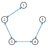
Figure 1: Network topology of five RL agents.

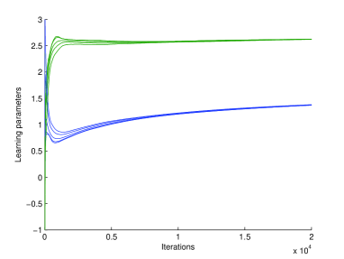
Figure 2: Evolution of iterates of the proposed DGTD (solid lines with different colors for different parameters), Algorithm 1. We use the step-size rule $\alpha_{k}=10/\sqrt{k+100}$ and $\kappa=1$.

Figure 2 depicts evolutions of two parameter iterates of the proposed DGTD (different colors for different parameters), Algorithm 1. It shows that the parameters of five agents reach a consensus and converge to certain numbers. The results empirically demonstrate the proposed DGTD.

Example 2.

Consider a $20[{\rm m}]\times 20[{\rm m}]$ continuous space $\mathcal{X}$ with three robots (agent 1 (blue), agent 2 (red), and agent 3 (black)), which patrol the space with identical stochastic motion planning policies $\pi_{1}=\pi_{2}=\pi_{3}=\pi$. We consider a single integrator system for each agent $i$: $\dot{x}_{i}(t)=u_{i}(t)$ with the control policy $u_{i}(t)=-h(x_{i}(t)-r_{i})$ employed from [42], where $t\in{\mathbb{R}}_{+}$ is the continuous time, $h\in{\mathbb{R}}_{++}$ is a constant, $r_{i}$ is a randomly chosen point in $\mathcal{X}$ with uniform distribution over $\mathcal{X}$. Under the control policy $u_{i}(t)=-h(x_{i}(t)-r_{i})$, $x_{i}(t)$ globally converges to $r_{i}$ as $t\to\infty$ [42, Lemma 1]. When $x_{i}$ is sufficiently close to the destination $r_{i}$, then it chooses another destination $r_{i}$ uniformly in $\mathcal{X}$, and all agents randomly maneuver the space $\mathcal{X}$. The continuous space $\mathcal{X}$ is discretized into the $20\times 20$ grid world $\mathcal{S}$. The collaborative objective of the three robots is to identify the dangerous region using individually collected reward (risk) information by each robot. The global value function estimated by the proposed distributed GTD learning informs the location of the points of interest. The three robots maneuver the space and detect the dangers together. For instance, these regions represent those with frequent turbulence in commercial flight routes or enemies in battle fields. Each robot is equipped with a different sensor that can detect different regions, while a pair of robots can exchange their parameters, when the distance between them is less than or equal to $5$. We assume that robots do not interfere with each other; thereby we can consider three independent MDPs with identical transition models.

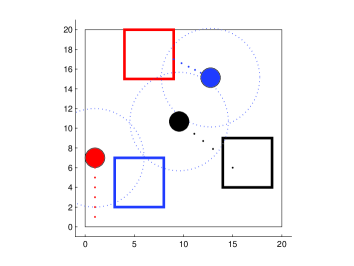
Figure 3: Three dangerous regions that can be detected by three different UAVs.

The three regions and robots are depicted in Figure 3, where the blue region is detected only by agent 1 (blue circle), the red region is detected only by agent 2 (red circle), and the black region only by agent 3 (black circle).

For each agent, the detection occurs only if the UAV flies over the region, and a reward $\hat{r}=100$ is given in this case. In the scenario above, the reward is given, when turbulence is detected: Algorithm 1 is applied with $\gamma=0.5$ and $\Phi=I_{|{\mathcal{S}}|}$ (tabular representation). We run Algorithm 1 with 50000 iterations, and the results are shown in Figure 4. The results suggest that all agents successfully estimate identical value functions, which are aware of three regions despite of the incomplete sensing abilities and communications. The obtained value function can be used to design a motion planning policy to travel safer routes.

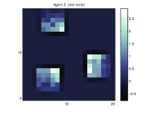
Figure 4: Example 2. 2D plots of value functions of three different agents.

9 Conclusion

In this paper, we study a distributed GTD learning for multi-agent MDPs using a stochastic primal-dual algorithm. Each agent receives local reward through a local processing, while information exchange over random communication networks allows them to learn the global value function corresponding to a sum of local rewards. Possible future research includes its extension to actor-critic and Q-learning algorithms.

Appendix

Appendix A Proof of Proposition 2

In this section, we will provide a proof of Proposition 2. We begin with a basic technical lemma.

Lemma 3 (Basic iterate relations [12]).

Let the sequences $(x_{k},w_{k})_{k=0}^{\infty}$ be generated by the stochastic subgradient algorithm in (9) and (10). Then, we have:

1. For any $x\in{\mathcal{X}}$ and for all $k\geq 0$,

   $${\mathbb{E}}[\|x_{k+1}-x\|^{2}|{\mathcal{F}}_{k}]$$

   $$\leq \|x_{k}-x\|^{2}+\alpha_{k}^{2}{\mathbb{E}}[\|{\mathcal{L}}_{x}(x_{k},w_{k})+\varepsilon_{k}\|^{2}|{\mathcal{F}}_{k}]$$

   $$-2\alpha_{k}({\mathcal{L}}(x_{k},w_{k})-{\mathcal{L}}(x,w_{k})).$$

2. For any $w\in{\mathcal{W}}$ and for all $k\geq 0$,

   $${\mathbb{E}}[\|w_{k+1}-w\|^{2}|{\mathcal{F}}_{k}]$$

   $$\leq \|w_{k}-w\|^{2}+\alpha_{k}^{2}{\mathbb{E}}[\|{\mathcal{L}}_{w}(x_{k},w_{k})+\xi_{k}\|^{2}|{\mathcal{F}}_{k}]$$

   $$+2\alpha_{k}({\mathcal{L}}(x_{k},w_{k})-{\mathcal{L}}(x_{k},w)).$$

Proof.

The result can be obtained by the iterate relations in [12, Lemma 3.1] and taking the expectations. ∎

Lemma 4 (Berstein inequality for Martingales [bercu2015concentration]).

Let $({\mathcal{M}}_{T})_{T=0}^{\infty}$ be a square integrable martingale such that ${\mathcal{M}}_{0}=0$. Assume that $\Delta{\mathcal{M}}_{T}\leq b,\forall T\geq 1$ with probability one, where $b>0$ is a real number and $\Delta{\mathcal{M}}_{T}$ is the Martingale difference defined as $\Delta{\mathcal{M}}_{T}:={\mathcal{M}}_{T}-{\mathcal{M}}_{T-1},T\geq 1$. Then, for any $\varepsilon\in[0,b]$ and $a>0$,

$${\mathbb{P}}\left[\frac{1}{T}{\mathcal{M}}_{T}\geq\varepsilon,\frac{1}{T}\left\langle{\mathcal{M}}\right\rangle_{T}\leq a\right]\leq\exp\left(-\frac{T\varepsilon^{2}}{2(a+b\varepsilon/3)}\right),$$

where

$$\langle{\mathcal{M}}\rangle_{T}:= \sum_{k=0}^{T-1}{\mathbb{E}}[\Delta{\mathcal{M}}_{k+1}^{2}|{\mathcal{F}}_{k}].$$

For any $x\in{\mathcal{X}}$ and $y\in{\mathcal{Y}}$, define

$${\mathcal{E}}_{k}^{(1)}(x):=\|x_{k}-x\|_{2}^{2},$$

$${\mathcal{E}}_{k}^{(2)}(w):=\|w_{k}-w\|_{2}^{2}$$

and

$$H_{k}(x):=\frac{1}{2\alpha_{k}}({\mathcal{E}}_{k}^{(1)}(x)-{\mathbb{E}}[{\mathcal{E}}_{k+1}^{(1)}(x)|{\mathcal{F}}_{k}]),$$

$$R_{k}(w):=\frac{1}{2\alpha_{k}}({\mathcal{E}}_{k}^{(2)}(y)-{\mathbb{E}}[{\mathcal{E}}_{k+1}^{(2)}(y)|{\mathcal{F}}_{k}]),$$

We use ${\mathbb{E}}[\|{\mathcal{L}}_{x}(x_{k},w_{k})+\varepsilon_{k}\|_{2}^{2}|{\mathcal{F}}_{k}]\leq C^{2}$ and rearrange terms in Lemma 3 to have

$${\mathcal{L}}(x_{k},y_{k})-{\mathcal{L}}(x,w_{k})$$

$$\leq \underbrace{\frac{1}{2\alpha_{k}}({\mathcal{E}}_{k}^{(1)}(x)-{\mathbb{E}}[{\mathcal{E}}_{k+1}^{(1)}(x)|{\mathcal{F}}_{k}])}_{=:H_{k}(x)}+\frac{\alpha_{k}}{2}C^{2},$$

$$\forall x\in{\mathbb{R}}^{|{\mathcal{S}}||{\mathcal{A}}|}\times{\mathbb{R}}^{|{\mathcal{S}}|},$$ (39)

$$-\underbrace{\frac{1}{2\alpha_{k}}({\mathcal{E}}_{k}^{(2)}(w)-{\mathbb{E}}[{\mathcal{E}}_{k+1}^{(2)}(w)|{\mathcal{F}}_{k}])}_{=:R_{k}(w)}-\frac{\alpha_{k}}{2}C^{2}$$

$$\leq {\mathcal{L}}(x_{k},w_{k})-{\mathcal{L}}(x_{k},w),\quad\forall w\in{\mathbb{R}}_{+}^{|{\mathcal{S}}||{\mathcal{A}}|}\times{\mathbb{R}}^{|{\mathcal{S}}||{\mathcal{A}}|}.$$ (40)

Adding these relations over $k=0,\ldots,T-1$, dividing by $T$, and rearranging terms, we have

$$-\frac{1}{T}\sum_{k=0}^{T-1}{R_{k}(w)}-\frac{1}{T}\sum_{k=0}^{T-1}{\frac{\alpha_{k}}{2}C^{2}}$$

$$\leq \frac{1}{T}\sum_{k=0}^{T-1}{({\mathcal{L}}(x_{k},w_{k})-{\mathcal{L}}(x_{k},w))},\quad\forall w\in{\mathcal{W}}.$$ (41)

Similarly, we have from (39)

$$\frac{1}{T}\sum_{k=0}^{T-1}{({\mathcal{L}}(x_{k},w_{k})-{\mathcal{L}}(x,w_{k}))}$$

$$\leq \frac{1}{T}\sum_{k=0}^{T-1}{H_{k}(x)}+\frac{1}{T}\sum_{k=0}^{T-1}{\frac{\alpha_{k}}{2}C^{2}},\quad\forall x\in{\mathcal{X}}.$$ (42)

Multiplying both sides of (41) by $-1$ and adding it with (42) yields

$$\frac{1}{T}\sum_{k=0}^{T-1}{({\mathcal{L}}(x_{k},w)-{\mathcal{L}}(x,w_{k}))}$$

$$\leq \frac{1}{T}\sum_{k=0}^{T-1}{R_{k}(w)}+\frac{1}{T}\sum_{k=0}^{T-1}{H_{k}(x)}+\frac{C^{2}}{T}\sum_{k=0}^{T-1}{\alpha_{k}}.$$

Using the convexity of ${\mathcal{L}}$ with respect to the first argument and the concavity of ${\mathcal{L}}$ with respect to the second argument, it follows from the last inequality that

$${\mathcal{L}}(\hat{x}_{T},w)-{\mathcal{L}}(x,\hat{w}_{T})$$

$$\leq \frac{1}{T}\sum_{k=0}^{T-1}{R_{k}(w)}+\frac{1}{T}\sum_{k=0}^{T-1}{H_{k}(x)}+\frac{C^{2}}{T}\sum_{k=0}^{T-1}{\alpha_{k}}.$$

To proceed, we rearrange terms in the last inequality to have

$${\mathcal{L}}(\hat{x}_{T},w)-{\mathcal{L}}(x,\hat{w}_{T})$$

$$\leq \frac{1}{T}\Phi_{1}(x)+\frac{1}{T}\Phi_{2}(y)+\frac{1}{T}{\mathcal{M}}_{T}+\frac{C^{2}}{T}\sum_{k=0}^{T-1}{\alpha_{k}},$$

$$\forall x\in{\mathcal{X}},w\in{\mathcal{W}},$$ (43)

where

$$\Phi_{1}(x):= \sum_{k=0}^{T-1}{\frac{1}{2\alpha_{k}}({\mathcal{E}}_{k}^{(1)}(x)-{\mathcal{E}}_{k+1}^{(1)}(x))},$$

$$\Phi_{2}(w):= \sum_{k=0}^{T-1}{\frac{1}{2\alpha_{k}}({\mathcal{E}}_{k}^{(2)}(w)-{\mathcal{E}}_{k+1}^{(2)}(w))},$$

$${\mathcal{M}}_{T}:= \sum_{k=0}^{T-1}\frac{1}{2\alpha_{k}}({\mathcal{E}}_{k+1}^{(1)}(x)+{\mathcal{E}}_{k+1}^{(2)}(w)$$

$$-{\mathbb{E}}[{\mathcal{E}}_{k+1}^{(1)}(x)|{\mathcal{F}}_{k}]-{\mathbb{E}}[{\mathcal{E}}_{k+1}^{(2)}(w)|{\mathcal{F}}_{k}]).$$

As a next step, we derive bounds on the terms $\Phi_{1}(x)$ and $\Phi_{2}(w)$. First, $\Phi_{1}(x)$ is bounded by using the chains of inequalities

$$\Phi_{1}(x) =\sum_{k=0}^{T-1}{\frac{1}{2\gamma_{k}}({\mathcal{E}}_{k}^{(1)}(x)-{\mathcal{E}}_{k+1}^{(1)}(x))}$$

$$\leq\sum_{k=0}^{T-1}{\frac{1}{2\gamma_{k}}({\mathcal{E}}_{k}^{(1)}(x)-{\mathcal{E}}_{k+1}^{(1)}(x))}+\frac{1}{\gamma_{T}}{\mathcal{E}}_{T}^{(1)}(x)$$

$$=\frac{1}{2}\left(\frac{1}{\gamma_{0}}{\mathcal{E}}_{0}^{(1)}(x)+\sum_{k=0}^{T-1}{\left(\frac{1}{\gamma_{k+1}}-\frac{1}{\gamma_{k}}\right){\mathcal{E}}_{k+1}^{(1)}(x)}\right)$$

$$\leq\frac{C^{2}}{2}\left(\frac{1}{\gamma_{0}}+\sum_{k=0}^{T-1}{\left(\frac{1}{\gamma_{k+1}}-\frac{1}{\gamma_{k}}\right)}\right)$$ (44)

$$=\frac{C^{2}}{2}{\gamma_{T}},$$

where (51) is due to ${\mathcal{E}}_{k}^{(1)}(x)\leq C^{2},\forall x\in{\mathcal{X}}$. Similarly, we have $\Phi_{2}(w)\leq\frac{C^{2}}{2}{\alpha_{T}}$. Combining the last inequality with (43) yields

$${\mathcal{L}}(\hat{x}_{T},w)-{\mathcal{L}}(x,\hat{w}_{T})\leq\frac{1}{T}\frac{C^{2}}{\gamma_{T}}+\frac{C^{2}}{T}\sum_{k=0}^{T-1}{\gamma_{k}}+\frac{1}{T}{\mathcal{M}}_{T},$$

$$\forall x\in{\mathcal{X}},w\in{\mathcal{W}},$$ (45)

Plugging $\alpha_{k}=\alpha_{0}/\sqrt{k+1}$ into the first term, we have

$$\frac{C^{2}}{T\alpha_{T}}=\frac{C^{2}\sqrt{T+1}}{T\alpha_{0}}\leq\frac{C^{2}\sqrt{T}+1}{T\alpha_{0}}=\frac{{C^{2}\sqrt{T}}}{T\alpha_{0}}+\frac{C^{2}}{T\alpha_{0}}$$

$$\leq\frac{C^{2}}{\sqrt{T}\alpha_{0}}+\frac{C^{2}}{\sqrt{T}\alpha_{0}}=\frac{2C^{2}}{\sqrt{T}\alpha_{0}}.$$

Moreover, plugging $\alpha_{k}=\alpha_{0}/\sqrt{k+1}$ into the second term leads to

$$\frac{1}{T}\sum_{k=0}^{T-1}{\alpha_{k}}=\frac{\alpha_{0}}{T}\sum_{k=1}^{T}{\frac{1}{\sqrt{k}}}\leq\frac{\alpha_{0}}{T}\int_{0}^{T}{\frac{1}{\sqrt{t}}dt}=\frac{\alpha_{0}\sqrt{T}}{T}=\frac{\alpha_{0}}{\sqrt{T}}.$$

Therefore, combining the bounds yields

$${\mathcal{L}}(\hat{x}_{T},w)-{\mathcal{L}}(x,\hat{w}_{T})\leq\frac{2C^{2}\alpha_{0}^{-1}+C^{2}\alpha_{0}}{\sqrt{T}}+\frac{1}{T}{\mathcal{M}}_{T}.$$ (46)

To prove ${\mathcal{L}}(\hat{x}_{T},w)-{\mathcal{L}}(x,\hat{w}_{T})\leq\varepsilon$, it suffices to prove $\frac{2C^{2}\alpha_{0}^{-1}+C^{2}\alpha_{0}}{\sqrt{T}}\leq\varepsilon/2$ and $\frac{1}{T}{\mathcal{M}}_{T}\leq\varepsilon/2$. By simple algebraic manipulations, we can prove that the first inequality holds if

$$T\geq \frac{4C^{4}(2\alpha_{0}^{-1}+\alpha_{0})^{2}}{\varepsilon^{2}}.$$ (47)

To prove the second inequality with high probability, we will use the Bernstein inequality in Lemma 4. To do so, one easily proves that ${\mathbb{E}}[{\mathcal{M}}_{T+1}|{\mathcal{F}}_{T}]={\mathcal{M}}_{T}$, and hence, $({\mathcal{M}}_{T})_{T=0}^{\infty}$ is a Martingale. Moreover, we will find constants $a>0$ and $b>0$ such that $\Delta{\mathcal{M}}_{T+1}:={\mathcal{M}}_{T+1}-{\mathcal{M}}_{T}\leq b$ and $\frac{1}{T}\langle{\mathcal{M}}\rangle_{T}\leq a$. Noting that ${\mathcal{M}}_{T+1}-{\mathcal{M}}_{T}=\frac{1}{2\alpha_{T}}({\mathcal{E}}_{T+1}^{(1)}-{\mathbb{E}}[{\mathcal{E}}_{T+1}^{(1)}|{\mathcal{F}}_{T}])+\frac{1}{2\alpha_{T}}({\mathcal{E}}_{T+1}^{(2)}-{\mathbb{E}}[{\mathcal{E}}_{T+1}^{(2)}|{\mathcal{F}}_{T}])$, we obtain the bounds for the first two terms

$$\frac{1}{2\alpha_{k}}({\mathcal{E}}_{k+1}^{(1)})-{\mathbb{E}}[{\mathcal{E}}_{k+1}^{(1)}|{\mathcal{F}}_{k}])$$ (48)

$$= \frac{1}{2\alpha_{k}}\|\Gamma_{\mathcal{X}}(x_{k}-\alpha_{k}{\mathcal{L}}_{x}(x_{k},w_{k})-\alpha_{k}\varepsilon_{k})-x^{*}\|^{2}$$

$$-\frac{1}{2\alpha_{k}}{\mathbb{E}}[\|\Gamma_{\mathcal{X}}(x_{k}-\alpha_{k}{\mathcal{L}}_{x}(x_{k},w_{k})-\alpha_{k}\varepsilon_{k})-x^{*}\|^{2}|{\mathcal{F}}_{k}]$$

$$= \frac{1}{2\alpha_{k}}(\|\Gamma_{\mathcal{X}}(x_{k}-\alpha_{k}{\mathcal{L}}_{x}(x_{k},w_{k})-\alpha_{k}\varepsilon_{k})-x_{k}\|_{2}^{2}+\|x_{k}-x^{*}\|_{2}^{2}$$

$$-2(x_{k}-x^{*})^{T}(\Gamma_{\mathcal{X}}(x_{k}-\alpha_{k}{\mathcal{L}}_{x}(x_{k},w_{k})-\alpha_{k}\varepsilon_{k})-x_{k})$$

$$-{\mathbb{E}}[\|\Gamma_{\mathcal{X}}(x_{k}-\alpha_{k}{\mathcal{L}}_{x}(x_{k},w_{k})-\alpha_{k}\varepsilon_{k})-x_{k}\|_{2}^{2}|{\mathcal{F}}_{k}]$$

$$-\|x_{k}-x^{*}\|_{2}^{2}$$

$$-{\mathbb{E}}[(\Gamma_{\mathcal{X}}(x_{k}-\alpha_{k}{\mathcal{L}}_{x}(x_{k},w_{k})-\alpha_{k}\varepsilon_{k})-x_{k})^{T}$$

$$\times(x_{k}-x^{*})|{\mathcal{F}}_{k}])$$ (49)

$$\leq \frac{1}{2\alpha_{k}}\|\Gamma_{\mathcal{X}}(x_{k}-\alpha_{k}{\mathcal{L}}_{x}(x_{k},w_{k})-\alpha_{k}\varepsilon_{k})-x_{k}\|_{2}^{2}$$

$$+\frac{1}{\alpha_{k}}\|x_{k}-x^{*}\|_{2}$$

$$\times\|\Gamma_{\mathcal{X}}(x_{k}-\alpha_{k}{\mathcal{L}}_{x}(x_{k},w_{k})-\alpha_{k}\varepsilon_{k})-x_{k}\|_{2}$$

$$+\frac{1}{\alpha_{k}}{\mathbb{E}}[\|x_{k}-x^{*}\|_{2}$$

$$\times\|\Gamma_{\mathcal{X}}(x_{k}-\alpha_{k}{\mathcal{L}}_{x}(x_{k},w_{k})-\alpha_{k}\varepsilon_{k})-x_{k}\|_{2}|{\mathcal{F}}_{k}]$$ (50)

$$\leq \frac{\alpha_{k}}{2}\|{\mathcal{L}}_{x}(x_{k},w_{k})+\varepsilon_{k}\|_{2}^{2}+\|x_{k}-x^{*}\|_{2}\|{\mathcal{L}}_{x}(x_{k},w_{k})+\varepsilon_{k}\|_{2}$$

$$+\|x_{k}-x^{*}\|_{2}{\mathbb{E}}[\|{\mathcal{L}}_{x}(x_{k},w_{k})+\varepsilon_{k}\|_{2}|{\mathcal{F}}_{k}]$$ (51)

$$\leq \alpha_{k}C^{2}/2+2C^{2},$$

where (49) follows from the relation $\|a-b\|_{2}^{2}=\|a\|_{2}^{2}+\|b\|_{2}^{2}-2a^{T}b$ for any vectors $a,b$, (50) follows from the Cauchy-Schwarz inequality, (51) follows from the nonexpansive map property of the projection $\|\Gamma_{\mathcal{X}}(a)-\Gamma_{\mathcal{X}}(b)\|_{2}\leq\|a-b\|_{2}$, and the last inequality is obtained after simplifications. Similarly, one gets $\frac{1}{2\alpha_{k}}({\mathcal{E}}_{k+1}^{(2)}-{\mathbb{E}}[{\mathcal{E}}_{k+1}^{(2)}|{\mathcal{F}}_{k}])\leq\alpha_{k}C^{2}/2+2C^{2}$. Combining the last two inequalities, we have $\Delta{\mathcal{M}}_{T+1}:={\mathcal{M}}_{T+1}-{\mathcal{M}}_{T}=\frac{1}{2\alpha_{T}}({\mathcal{E}}_{T+1}-{\mathbb{E}}[{\mathcal{E}}_{T+1}|{\mathcal{F}}_{T}])\leq b$ with probability one, where $b=\alpha_{0}C^{2}+4C^{2}$.

Next, we will prove that $\frac{1}{T}\langle{\mathcal{M}}\rangle_{T}\leq a$ holds, where $a=(\alpha_{0}+2)^{2}C^{4}$. Using ${\mathbb{E}}[{\mathcal{E}}_{k}^{(1)}+{\mathcal{E}}_{k}^{(2)}|{\mathcal{F}}_{k}]={\mathcal{E}}_{k}^{(1)}+{\mathcal{E}}_{k}^{(2)}$, we have

$${\mathbb{E}}[|{\mathcal{M}}_{k+1}-{\mathcal{M}}_{k}|^{2}|{\mathcal{F}}_{k}]$$

$$= \frac{1}{4\alpha_{k}^{2}}{\mathbb{E}}[|{\mathcal{E}}_{k+1}-{\mathbb{E}}[{\mathcal{E}}_{k+1}|{\mathcal{F}}_{k}]|^{2}|{\mathcal{F}}_{k}]$$

$$= \frac{1}{4\alpha_{k}^{2}}{\mathbb{E}}[|{\mathcal{E}}_{k+1}-{\mathcal{E}}_{k}-{\mathbb{E}}[{\mathcal{E}}_{k+1}-{\mathcal{E}}_{k}|{\mathcal{F}}_{k}]|^{2}|{\mathcal{F}}_{k}]$$

$$\leq \frac{1}{4\alpha_{k}^{2}}{\mathbb{E}}[{\mathbb{E}}[|{\mathcal{E}}_{k+1}-{\mathcal{E}}_{k}|^{2}|{\mathcal{F}}_{k}]|{\mathcal{F}}_{k}]$$

$$= \frac{1}{4\gamma_{k}^{2}}{\mathbb{E}}[|\underbrace{{\mathcal{E}}_{k+1}^{(1)}+{\mathcal{E}}_{k+1}^{(2)}-{\mathcal{E}}_{k}^{(1)}-{\mathcal{E}}_{k}^{(2)}}_{=:\Phi_{1}}|^{2}|{\mathcal{F}}_{k}],$$ (52)

where the inequality follows from the fact that the variance of a random variable is bounded by its second moment. For bounding (52), note that $\Phi_{1}$ is written as

$$\Phi_{1}= \|x_{k+1}-x^{*}\|_{2}^{2}-\|x_{k}-x^{*}\|_{2}^{2}$$

$$+\|w_{k+1}-w^{*}\|_{2}^{2}-\|w_{k}-w^{*}\|_{2}^{2}.$$

Here, the first two terms have the bound

$$\|x_{k+1}-x^{*}\|^{2}-\|x_{k}-x^{*}\|^{2}$$

$$= \|\Gamma_{\mathcal{X}}(x_{k}-\alpha_{k}L_{x}(x_{k},w_{k})-\alpha_{k}\varepsilon_{k})-x_{k}\|^{2}$$

$$-2(\Gamma_{\mathcal{X}}(x_{k}-\alpha_{k}L_{x}(x_{k},w_{k})-\alpha_{k}\varepsilon_{k})-x_{k})^{T}(x_{k}-x^{*})$$ (53)

$$\leq \|\Gamma_{\mathcal{X}}(x_{k}-\alpha_{k}L_{x}(x_{k},w_{k})-\alpha_{k}\varepsilon_{k})-x_{k}\|_{2}^{2}$$

$$+2\|\Gamma_{\mathcal{X}}(x_{k}-\alpha_{k}L_{x}(x_{k},w_{k})-\alpha_{k}\varepsilon_{k})-x_{k}\|_{2}\|x_{k}-x^{*}\|_{2}$$ (54)

$$\leq \alpha_{k}^{2}\|L_{x}(x_{k},w_{k})+\varepsilon_{k}\|_{2}^{2}$$

$$+2\alpha_{k}\|L_{x}(x_{k},w_{k})+\varepsilon_{k}\|_{2}\|x_{k}-x^{*}\|_{2}$$ (55)

$$\leq \alpha_{k}(\alpha_{0}C^{2}+2C^{2}),$$ (56)

where (53) follows from the relation $\|a-b\|_{2}^{2}=\|a\|_{2}^{2}+\|b\|_{2}^{2}-2a^{T}b$ for any vectors $a,b$, (54) follows from the Cauchy-Schwarz inequality, (55) is due to the nonexpansive map property of the projection $\|\Gamma_{\mathcal{X}}(a)-\Gamma_{\mathcal{X}}(b)\|_{2}\leq\|a-b\|_{2}$, (56) comes from (11), (12), and (13). Similarly, the second two terms in $\Phi_{1}$ are bounded by $\alpha_{k}(\alpha_{0}C^{2}+2C^{2})$. Combining the last two results leads to $\Phi_{1}\leq 2\alpha_{k}(\alpha_{0}C^{2}+2C^{2})$, and plugging the bound on $\Phi_{1}$ into (52) and after simplifications, we obtain ${\mathbb{E}}[|{\mathcal{M}}_{k+1}-{\mathcal{M}}_{k}|^{2}|{\mathcal{F}}_{k}]\leq(\alpha_{0}+2)^{2}C^{4}$, which is the desired conclusion.

We are now ready to apply the Bernstein inequality in Lemma 4 to prove $\frac{1}{T}{\mathcal{M}}_{T}\leq\varepsilon/2$ with high probability. Fix any $x\in{\mathcal{X}},w\in{\mathcal{W}}$ and apply the Bernstein inequality with $a$ and $b$ given above to prove

$${\mathbb{P}}\left[\frac{1}{T}{\mathcal{M}}_{T}\geq\frac{\varepsilon}{2},\frac{1}{T}\langle{\mathcal{M}}\rangle_{T}\leq a\right]$$

$$= {\mathbb{P}}\left[\frac{1}{T}{\mathcal{M}}_{T}\geq\frac{\varepsilon}{2}\right]\leq\exp\left(-\frac{T\varepsilon^{2}}{8(a+b\varepsilon/6)}\right)$$

with any $\varepsilon>0$. Note that for any $\delta\in(0,1)$, $\exp\left(-\frac{T\varepsilon^{2}}{8(a+b\varepsilon/6)}\right)\leq\delta$ holds if and only if $T\geq\frac{8(a+b\varepsilon/6)}{\varepsilon^{2}}\ln(\delta^{-1})$. By plugging $a$ and $b$ given before into the last inequality, it holds that if

$$T\geq\frac{8C^{2}((\alpha_{0}+2)^{2}C^{2}+(\alpha_{0}+4)\varepsilon/6)}{\varepsilon^{2}}\ln\left(\frac{1}{\delta}\right),$$

then with probability at least $1-\delta$, we have ${\mathcal{M}}_{T}/T\leq\varepsilon/2$. Combined with (47), one concludes that under the conditions in the statement of Proposition 2, with probability at least $1-\delta$, ${\mathcal{L}}(\hat{x}_{T},w)-{\mathcal{L}}(x,\hat{w}_{T})\leq\varepsilon$ holds. By Definition 2, it implies

$${\mathbb{P}}[(\hat{x}_{T},\hat{w}_{T})\in{\mathcal{H}}_{\varepsilon}]\geq 1-\delta.$$

This completes the proof.

References

• [1] R. S. Sutton, H. R. Maei, and C. Szepesvári, “A convergent $o(n)$ temporal-difference algorithm for off-policy learning with linear function approximation,” in Advances in neural information processing systems, 2009, pp. 1609–1616.
• [2] R. S. Sutton, H. R. Maei, D. Precup, S. Bhatnagar, D. Silver, C. Szepesvári, and E. Wiewiora, “Fast gradient-descent methods for temporal-difference learning with linear function approximation,” in Proceedings of the 26th Annual International Conference on Machine Learning, 2009, pp. 993–1000.
• [3] A. Jadbabaie, J. Lin, and A. Morse, “Coordination of groups of mobile autonomous agents using nearest neighbor rules,” IEEE Transactions on Automatic Control, vol. 48, no. 6, pp. 988–1001, 2003.
• [4] J. Wang and N. Elia, “Control approach to distributed optimization,” in 48th Annual Allerton Conference on Communication, Control, and Computing (Allerton), 2010, pp. 557–561.
• [5] ——, “A control perspective for centralized and distributed convex optimization,” in 50th IEEE Conference on Decision and Control and European Control Conference (CDC-ECC), 2011, pp. 3800–3805.
• [6] B. Gharesifard and J. Cortés, “Distributed continuous-time convex optimization on weight-balanced digraphs,” IEEE Transactions on Automatic Control, vol. 59, no. 3, pp. 781–786, 2014.
• [7] W. Shi, Q. Ling, G. Wu, and W. Yin, “Extra: An exact first-order algorithm for decentralized consensus optimization,” SIAM Journal on Optimization, vol. 25, no. 2, pp. 944–966, 2015.
• [8] A. Mokhtari and A. Ribeiro, “DSA: Decentralized double stochastic averaging gradient algorithm,” Journal of Machine Learning Research, vol. 17, no. 61, pp. 1–35, 2016.
• [9] J. Lei, H.-F. Chen, and H.-T. Fang, “Primal–dual algorithm for distributed constrained optimization,” Systems & Control Letters, vol. 96, pp. 110–117, 2016.
• [10] A. Nemirovski, A. Juditsky, G. Lan, and A. Shapiro, “Robust stochastic approximation approach to stochastic programming,” SIAM Journal on optimization, vol. 19, no. 4, pp. 1574–1609, 2009.
• [11] Y. Chen and M. Wang, “Stochastic primal-dual methods and sample complexity of reinforcement learning,” arXiv preprint arXiv:1612.02516, 2016.
• [12] A. Nedić and A. Ozdaglar, “Subgradient methods for saddle-point problems,” Journal of optimization theory and applications, vol. 142, no. 1, pp. 205–228, 2009.
• [13] H.-T. Wai, Z. Yang, Z. Wang, and M. Hong, “Multi-agent reinforcement learning via double averaging primal-dual optimization,” in Advances in Neural Information Processing Systems, 2018, pp. 9649–9660.
• [14] D. Ding, X. Wei, Z. Yang, Z. Wang, and M. R. Jovanović, “Fast multi-agent temporal-difference learning via homotopy stochastic primal-dual optimization,” arXiv preprint arXiv:1908.02805, 2019.
• [15] S. Kar, J. M. Moura, and H. V. Poor, “QD-learning: a collaborative distributed strategy for multi-agent reinforcement learning through consensus $+$ innovations,” IEEE Transactions on Signal Processing, vol. 61, no. 7, pp. 1848–1862, 2013.
• [16] K. Zhang, Z. Yang, H. Liu, T. Zhang, and T. Başar, “Fully decentralized multi-agent reinforcement learning with networked agents,” arXiv preprint arXiv:1802.08757, 2018.
• [17] S. V. Macua, J. Chen, S. Zazo, and A. H. Sayed, “Distributed policy evaluation under multiple behavior strategies,” IEEE Transactions on Automatic Control, vol. 60, no. 5, pp. 1260–1274, 2015.
• [18] M. S. Stanković and S. S. Stanković, “Multi-agent temporal-difference learning with linear function approximation: weak convergence under time-varying network topologies,” in American Control Conference (ACC), 2016, pp. 167–172.
• [19] A. Mathkar and V. S. Borkar, “Distributed reinforcement learning via gossip,” IEEE Transactions on Automatic Control, vol. 62, no. 3, pp. 1465–1470, 2017.
• [20] W. Suttle, Z. Yang, K. Zhang, Z. Wang, T. Basar, and J. Liu, “A multi-agent off-policy actor-critic algorithm for distributed reinforcement learning,” arXiv preprint arXiv:1903.06372, 2019.
• [21] K. Zhang, Z. Yang, H. Liu, T. Zhang, and T. Basar, “Finite-sample analyses for fully decentralized multi-agent reinforcement learning,” arXiv preprint arXiv:1812.02783, 2018.
• [22] C. Qu, S. Mannor, H. Xu, Y. Qi, L. Song, and J. Xiong, “Value propagation for decentralized networked deep multi-agent reinforcement learning,” in Advances in Neural Information Processing Systems, 2019, pp. 1182–1191.
• [23] T. T. Doan, S. T. Maguluri, and J. Romberg, “Convergence rates of distributed td (0) with linear function approximation for multi-agent reinforcement learning,” arXiv preprint arXiv:1902.07393, 2019.
• [24] L. Cassano, K. Yuan, and A. H. Sayed, “Distributed value-function learning with linear convergence rates,” in European Control Conference (ECC), 2019, pp. 505–511.
• [25] G. Qu and N. Li, “Harnessing smoothness to accelerate distributed optimization,” IEEE Transactions on Control of Network Systems, vol. 5, no. 3, pp. 1245–1260, 2017.
• [26] D. Lee, H. Yoon, and N. Hovakimyan, “Primal-dual algorithm for distributed reinforcement learning: distributed GTD,” 57th IEEE Conference on Decision and Control, pp. 1967–1972, 2018.
• [27] H. Kushner and G. G. Yin, Stochastic approximation and recursive algorithms and applications.   Springer Science & Business Media, 2003, vol. 35.
• [28] D. P. Bertsekas, Nonlinear programming.   Athena scientific Belmont, 1999.
• [29] I. Lobel and A. Ozdaglar, “Distributed subgradient methods for convex optimization over random networks,” IEEE Transactions on Automatic Control, vol. 56, no. 6, pp. 1291–1306, 2011.
• [30] R. Olfati-Saber, “Flocking for multi-agent dynamic systems: Algorithms and theory,” IEEE Transactions on automatic control, vol. 51, no. 3, pp. 401–420, 2006.
• [31] R. S. Sutton and A. G. Barto, Reinforcement learning: An introduction.   MIT Press, 1998.
• [32] D. P. Bertsekas and J. N. Tsitsiklis, Neuro-dynamic programming.   Athena Scientific Belmont, MA, 1996.
• [33] G. A. Rummery and M. Niranjan, On-line Q-learning using connectionist systems.   University of Cambridge, Department of Engineering Cambridge, England, 1994, vol. 37.
• [34] V. R. Konda and J. N. Tsitsiklis, “Actor-critic algorithms,” in Advances in neural information processing systems, pp. 1008–1014.
• [35] A. Nedic, A. Ozdaglar, and P. A. Parrilo, “Constrained consensus and optimization in multi-agent networks,” IEEE Transactions on Automatic Control, vol. 55, no. 4, pp. 922–938, 2010.
• [36] S. Boyd and L. Vandenberghe, Convex Optimization.   Cambridge University Press, 2004.
• [37] A. Ghosh, S. Boyd, and A. Saberi, “Minimizing effective resistance of a graph,” SIAM review, vol. 50, no. 1, pp. 37–66, 2008.
• [38] D. P. Bertsekas, Convex optimization algorithms.   Athena Scientific Belmont, 2015.
• [39] S. Mahadevan, B. Liu, P. Thomas, W. Dabney, S. Giguere, N. Jacek, I. Gemp, and J. Liu, “Proximal reinforcement learning: a new theory of sequential decision making in primal-dual spaces,” arXiv preprint arXiv:1405.6757, 2014.
• [40] S. Ghadimi and G. Lan, “Stochastic first-and zeroth-order methods for nonconvex stochastic programming,” SIAM Journal on Optimization, vol. 23, no. 4, pp. 2341–2368, 2013.
• [41] Q. Lin, M. Liu, H. Rafique, and T. Yang, “Solving weakly-convex-weakly-concave saddle-point problems as successive strongly monotone variational inequalities,” arXiv preprint arXiv:1810.10207, 2018.
• [42] D. Panagou, M. Turpin, and V. Kumar, “Decentralized goal assignment and trajectory generation in multi-robot networks: A multiple lyapunov functions approach,” in Robotics and Automation (ICRA), 2014 IEEE International Conference on, 2014, pp. 6757–6762.