Holographic DC Conductivity for Backreacted Nonlinear Electrodynamics with Momentum Dissipation

Abstract

We consider a holographic model with the charge current dual to a general nonlinear electrodynamics (NLED) field. Taking into account the backreaction of the NLED field on the geometry and introducing axionic scalars to generate momentum dissipation, we obtain expressions for DC conductivities with a finite magnetic field. The properties of the in-plane resistance are examined in several NLED models. For Maxwell-Chern-Simons electrodynamics, negative magneto-resistance and Mott-like behavior could appear in some parameter space region. Depending on the sign of the parameters, we expect the NLED models to mimic some type of weak or strong interactions between electrons. In the latter case, negative magneto-resistance and Mott-like behavior can be realized at low temperatures. Moreover, the Mott insulator to metal transition induced by a magnetic field is also observed at low temperatures.

I Introduction

Gauge/gravity duality IN-Banks:1996vh ; IN-Maldacena:1997re ; IN-Witten:1998qj has provided powerful tools for exploring the behavior of strongly coupled quantum phases of matter, and some remarkable progresses have been made IN-Gubser:2008px ; IN-Hartnoll:2008vx ; IN-Lee:2008xf ; IN-Liu:2009dm ; IN-Cubrovic:2009ye . Conductivity is an important transport quantity in condensed matter, and the gauge/gravity duality provides a framework to compute it for strongly interacting field theories.

Studying the behavior of the conductivity in the presence of external magnetic fields can help us to better understand the transport properties of materials. For normal metals, the resistance is a monotonically increasing function of the magnetic field IN-Wannier1972 , which appears as positive magneto-resistance. However, negative magneto-resistance has been observed in several experiments IN-Negishi ; IN-Li ; IN-Kim . On the other hand, the behavior of negative magneto-resistance was found in strongly coupled holographic chiral anomalous systems IN-Jimenez-Alba:2014iia ; IN-Jimenez-Alba:2015awa ; IN-Landsteiner:2014vua ; IN-Sun:2016gpy . In IN-Baumgartner:2017kme , it showed that negative magneto-resistance could also arise in nonanomalous relativistic fluids due to the distinctive gradient expansion. Note that the transport phenomena in the presence of Weyl corrections have also been discussed in IN-Mokhtari:2017vyz ; IN-Chu:2018ksb ; Chu:2018ntx . Recently, the magnetotransport of a strongly interacting system in $2+1$ dimensions was examined in a holographic Dirac-Born-Infeld model in IN-Kiritsis:2016cpm ; IN-Cremonini:2017qwq . Negative magnetoresistance was found for a family of dynoic solutions in IN-Cremonini:2017qwq . The DC conductivity in the probe DBI case with the vanishing magnetic field was also discussed in IN-Charmousis:2010zz .

Mott insulators can be parent materials of high $T_{c}$ cuprate superconductors. A Mott insulator has an insulating ground state driven by Coulomb repulsion. Mott-like behavior is that strong interactions between electrons would prevent the charge carriers to efficiently transport charges. Constructing a holographic model describing Mott insulators is still a challenging task. In IN-Edalati:2010ww ; IN-Edalati:2010ge ; IN-Wu:2012fk ; IN-Ling:2014bda , dynamically generating a Mott gap has been proposed in holographic models by considering fermions with dipole coupling. A holographic construction of the large-$N$ Bose-Hubbard model was presented in IN-Fujita:2014mqa , and the model admitted Mott insulator ground states in the limit of large Coulomb repulsion. Some other holographic models dual to Mott insulators include IN-Ling:2015epa ; IN-Nishioka:2009zj ; IN-Kiritsis:2015oxa . Recently, a holographic model using a particular type of NLED, namely iDBI, was proposed in IN-Baggioli:2016oju to mimic interactions between electrons by self-interactions of the NLED field. It showed that Mott-like behavior appeared for large enough self-interaction strength.

In this paper, we extend the analysis of the magnetotransport in a holographic Dirac-Born-Infeld model in IN-Cremonini:2017qwq to a general NLED model. As in IN-Cremonini:2017qwq , our analysis is performed in a full backreacted fashion. To break translational symmetry, we follow the method in IN-Andrade:2013gsa to add axionic scalars, which depend on the spatial directions linearly.

The rest of this article is organized as follows. In section II, we set up our holographic model. The expressions for the DC conductivities with a finite magnetic field are obtained in section III. Some limiting cases, including high temperature limit, are then discussed. In section IV, the dependence of the in-plane resistance on the temperature, the charge density and the magnetic field are investigated for Maxwell, Maxwell-Chern-Simons, Born-Infeld, square and logarithmic electrodynamics. In section V, we summarize our results and conclude with a brief discussion.

II Holographic Setup

Consider a 4-dimensional model of gravity coupled to a nonlinear electromagnetic field $A_{a}$ and two axions $\psi_{I}$ with action given by

$$S=\int d^{4}x\sqrt{-g}\left[R-2\Lambda-\frac{1}{2}\sum_{I=1}^{2}\left(\partial\psi_{I}\right)^{2}+\mathcal{L}\left(s,p\right)\right],$$ (1)

where $\Lambda=-\frac{3}{l^{2}}$, and we take $16\pi G=1$ for simplicity. In the action $\left(\ref{eq:Action}\right)$, we assume that the generic NLED Lagrangian is $\mathcal{L}\left(s,p\right)$, where we build two independent nontrivial scalars using $F_{ab}=\partial_{a}A_{b}-\partial_{b}A_{a}$ and none of its derivatives:

$$s=-\frac{1}{4}F^{ab}F_{ab}\text{ and }p=-\frac{1}{8}\epsilon^{abcd}F_{ab}F_{cd}\text{;}$$ (2)

$\epsilon^{abcd}\equiv-\left[a\text{ }b\text{ }c\text{ }d\right]/\sqrt{-g}$ is a totally antisymmetric Lorentz tensor, and $\left[a\text{ }b\text{ }c\text{ }d\right]$ is the permutation symbol. We also assume that the NLED Lagrangian would reduce to the form of Maxwell-Chern-Simons Lagrangian for small fields:

$$\mathcal{L}\left(s,p\right)\approx s+\theta p,$$ (3)

where, for later convenience, we define $\theta\equiv\mathcal{L}^{\left(0,1\right)}\left(0,0\right)$. Note that we set the AdS radius $l=1$ hereafter.

Varying the action $\left(\ref{eq:Action}\right)$ with respect to $g_{ab}$, $A_{a}$, and $\psi_{I}$, we find that the equations of motion are

$$R_{ab}-\frac{1}{2}Rg_{ab}-\frac{3}{l^{2}}g_{ab} =\frac{T_{ab}}{2}\text{,}$$

$$\nabla_{a}G^{ab} =0\text{,}$$ (4)

$$\partial_{\mu}\left(\sqrt{-g}\partial^{\mu}\psi_{I}\right) =0\text{,}$$

where $T_{ab}$ is the energy-momentum tensor:

$$T_{ab}=g_{ab}\left[-\frac{1}{2}\sum_{I=1}^{2}\left(\partial\psi_{I}\right)^{2}+\mathcal{L}\left(s,p\right)-p\frac{\partial\mathcal{L}\left(s,p\right)}{\partial p}\right]+\sum_{I=1}^{2}\left(\partial_{a}\psi_{I}\right)\left(\partial_{b}\psi_{I}\right)+\frac{\partial\mathcal{L}\left(s,p\right)}{\partial s}F_{a}^{\text{ }c}F_{bc}\text{,}$$ (5)

and we define

$$G^{ab}=-\frac{\partial\mathcal{L}\left(s,p\right)}{\partial F_{ab}}=\frac{\partial\mathcal{L}\left(s,p\right)}{\partial s}F^{ab}+\frac{1}{2}\frac{\partial\mathcal{L}\left(s,p\right)}{\partial p}\epsilon^{abcd}F_{cd}.$$ (6)

To construct a black brane solution with asymptotic AdS spacetime, we take the following ansatz for the metric, the NLED field and the axions

$$ds^{2} =-f\left(r\right)dt^{2}+\frac{dr^{2}}{f\left(r\right)}+r^{2}\left(dx^{2}+dy^{2}\right)\text{,}$$

$$A =A_{t}\left(r\right)dt+\frac{h}{2}\left(xdy-ydx\right)\text{,}$$ (7)

$$\psi_{1} =\alpha x\text{, and }\psi_{2}=\alpha y\text{,}$$

where $h$ denotes the magnitude of the magnetic field. The axions are responsible for the breaking the translational invariance and generating momentum dissipation. The equations of motion then take the form:

$$f\left(r\right)-3r^{2}+rf^{\prime}\left(r\right) =-\frac{\alpha^{2}}{2}+\frac{r^{2}}{2}\left[\mathcal{L}\left(s,p\right)+A_{t}^{\prime}\left(r\right)G^{rt}\right],$$ (8)

$$2f^{\prime}\left(r\right)-6r+rf^{\prime\prime}\left(r\right) =r\left[\mathcal{L}\left(s,p\right)+hG^{xy}\right],$$ (9)

$$\left[r^{2}G^{rt}\right]^{\prime} =0\text{.}$$ (10)

It can be shown that eqns. $\left(\ref{eq:ttEOM}\right)$ and $\left(\ref{eq:NLEDEOM}\right)$ guarantee that eqn. $\left(\ref{eq:rrEOM}\right)$ always holds. Eqn. $\left(\ref{eq:NLEDEOM}\right)$ leads to

$$G^{tr}=\frac{\rho}{r^{2}}\text{,}$$ (11)

where $\rho$ is a constant. One has $f\left(r_{h}\right)=0$ at the horizon $r=r_{h}$, and the Hawking temperature of the black brane is given by

$$T=\frac{f^{\prime}\left(r_{h}\right)}{4\pi}\text{.}$$ (12)

Hence at $r=r_{h}$, eqn. $\left(\ref{eq:ttEOM}\right)$ reduces to

$$-3r_{h}^{2}+4\pi r_{h}T=-\frac{\alpha^{2}}{2}+\frac{r_{h}^{2}}{2}\left[\mathcal{L}\left(s_{h},p_{h}\right)+A_{t}^{\prime}\left(r_{h}\right)G_{h}^{rt}\right],$$ (13)

where

$$s_{h} =\frac{A_{t}^{\prime 2}\left(r_{h}\right)}{2}-\frac{h^{2}}{2r_{h}^{4}}\text{,}$$

$$\text{ }p_{h} =-\frac{hA_{t}^{\prime}\left(r_{h}\right)}{r_{h}^{2}}\text{,}$$ (14)

$$G_{h}^{rt} =-\mathcal{L}^{\left(1,0\right)}\left(s_{h},p_{h}\right)A_{t}^{\prime}\left(r_{h}\right)+\mathcal{L}^{\left(0,1\right)}\left(s_{h},p_{h}\right)\frac{h}{r_{h}^{2}}\text{.}$$

III DC Conductivity

Via gauge/gravity duality, the black brane solution $\left(\ref{eq:BBAnsatz}\right)$ describes an equilibrium state at finite temperature $T$, which is given by eqn. $\left(\ref{eq:HT}\right)$. The NLED field is a U$\left(1\right)$ gauge field and dual to a conserved current $\mathcal{J}^{\mu}$ in the boundary theory. In this section, we calculate the DC conductivities for $\mathcal{J}^{\mu}$ using the method developed in In-Donos:2014uba ; IN-Blake:2014yla .

III.1 Derivation of DC Conductivity

To calculate the DC conductivities, we consider the perturbations of the form:

$$\delta g_{ti}=r^{2}h_{ti}\left(r\right)\text{, }\delta g_{ri}=r^{2}h_{ri}\left(r\right)\text{, }\delta A_{i}=-E_{i}t+a_{i}\left(r\right)\text{, }\delta\psi_{I}=\chi_{I}\left(r\right)\text{,}$$ (15)

where $i=x$, $y$ and $I=1,2$. The fields $a_{i}\left(r\right)$ do not appear explicitly in the NLED Lagrangian $\mathcal{L}\left(s,p\right)$. Thus, the conjugate momentum of the field $a_{i}\left(r\right)$ with respect to $r$-foliation is radially independent:

$$\partial_{r}\Pi^{i}=0\text{,}$$ (16)

where the conjugate current is

$$\Pi^{i}=\frac{\partial\mathcal{L}\left(s,p\right)}{\partial\left(a_{i}^{\prime}\left(r\right)\right)}=\frac{\partial\mathcal{L}\left(s,p\right)}{\partial\left(\partial_{r}A_{i}\right)}=\sqrt{-g}G^{ir}.$$ (17)

Similarly, the conjugate momentum of the field $A_{t}\left(r\right)$ is also a constant flux

$$\partial_{r}\Pi^{t}=0\text{,}$$ (18)

where one has

$$\Pi^{t}=\frac{\partial\mathcal{L}\left(s,p\right)}{\partial\left(A_{t}^{\prime}\left(r\right)\right)}.$$ (19)

We can then compute the expectation value of $\mathcal{J}^{t}$ for the boundary theory by

$$\left\langle\mathcal{J}^{t}\right\rangle=\Pi^{t}.$$ (20)

Using eqns. $\left(\ref{eq:Gab}\right)$, $\left(\ref{eq:BBAnsatz}\right)$, $\left(\ref{eq:Grt}\right)$, $\left(\ref{eq:purb}\right)$, and $\left(\ref{eq:Pit}\right)$, we find that, at the linearized order,

$$\left\langle\mathcal{J}^{t}\right\rangle=\rho\text{,}$$ (21)

which means that $\rho$ can be interpreted as the charge density in the dual field theory. Evaluating eqn. $\left(\ref{eq:Pit}\right)$ at $r=r_{h}$ gives

$$\rho=\mathcal{L}^{\left(1,0\right)}\left(s_{h},p_{h}\right)A_{t}^{\prime}\left(r_{h}\right)-\mathcal{L}^{\left(0,1\right)}\left(s_{h},p_{h}\right)\frac{h}{r_{h}^{2}}.$$ (22)

The charge currents in the dual theory are given by

$$\left\langle\mathcal{J}^{i}\right\rangle=\Pi^{i}\text{,}$$ (23)

which lead to

$$\left\langle\mathcal{J}^{x}\right\rangle =-\mathcal{L}^{\left(1,0\right)}\left(s,p\right)\left[f\left(r\right)a_{x}^{\prime}\left(r\right)+hf\left(r\right)h_{ry}\left(r\right)+r^{2}A_{t}^{\prime}\left(r\right)h_{tx}\left(r\right)\right]-\mathcal{L}^{\left(0,1\right)}\left(s,p\right)E_{y}\text{,}$$

$$\left\langle\mathcal{J}^{y}\right\rangle =-\mathcal{L}^{\left(1,0\right)}\left(s,p\right)\left[f\left(r\right)a_{y}^{\prime}\left(r\right)-hf\left(r\right)h_{rx}\left(r\right)+r^{2}A_{t}^{\prime}\left(r\right)h_{ty}\left(r\right)\right]+\mathcal{L}^{\left(0,1\right)}\left(s,p\right)E_{x}\text{.}$$ (24)

To express $\left\langle\mathcal{J}^{i}\right\rangle$ in terms of $E_{i}$, we first consider the constraints of regularity on the metric and fields around the horizon IN-Blake:2014yla :

$$f\left(r\right) =4\pi T\left(r-r_{h}\right)+\cdots\text{,}$$

$$A_{t}\left(r\right) =A_{t}^{\prime}\left(r_{h}\right)\left(r-r_{h}\right)+\cdots\text{,}$$

$$a_{i}\left(r\right) =-\frac{E_{i}}{4\pi T}\ln\left(r-r_{h}\right)+\cdots\text{,}$$ (25)

$$h_{ri}\left(r\right) =\frac{h_{ti}\left(r\right)}{f\left(r\right)}+\cdots\text{,}$$

$$\chi_{I}\left(r\right) =\chi_{I}\left(r_{h}\right)+\cdots\text{.}$$

We then consider the $tx$ and $ty$ component of the perturbed Einstein’s equations:

$$h_{tx}\left(r\right)\left[-\frac{\alpha^{2}}{\mathcal{L}^{\left(1,0\right)}\left(s,p\right)}-\frac{h^{2}}{r^{2}}\right]-\frac{hE_{y}}{r^{2}}+A_{t}^{\prime}\left(r\right)f\left(r\right)\left[a_{x}^{\prime}\left(r\right)+hh_{ry}\left(r\right)\right] =0,$$

$$h_{ty}\left(r\right)\left[-\frac{\alpha^{2}}{\mathcal{L}^{\left(1,0\right)}\left(s,p\right)}-\frac{h^{2}}{r^{2}}\right]+\frac{hE_{x}}{r^{2}}+A_{t}^{\prime}\left(r\right)f\left(r\right)\left[a_{y}^{\prime}\left(r\right)-hh_{rx}\left(r\right)\right] =0\text{.}$$ (26)

Using the regularity conditions $\left(\ref{eq:reg}\right)$, eqns. $\left(\ref{eq:txty}\right)$ reduce to

$$hA_{t}^{\prime}\left(r_{h}\right)h_{ty}\left(r_{h}\right)-\left[\frac{\alpha^{2}}{\mathcal{L}^{\left(1,0\right)}\left(s_{h},p_{h}\right)}+\frac{h^{2}}{r_{h}^{2}}\right]h_{tx}\left(r_{h}\right) =A_{t}^{\prime}\left(r_{h}\right)E_{x}+\frac{hE_{y}}{r_{h}^{2}}\text{,}$$

$$hA_{t}^{\prime}\left(r_{h}\right)h_{tx}\left(r_{h}\right)+\left[\frac{\alpha^{2}}{\mathcal{L}^{\left(1,0\right)}\left(s_{h},p_{h}\right)}+\frac{h^{2}}{r_{h}^{2}}\right]h_{ty}\left(r_{h}\right) =\frac{hE_{x}}{r_{h}^{2}}-A_{t}^{\prime}\left(r_{h}\right)E_{y}\text{,}$$ (27)

where $s_{h}$ and $p_{h}$ are given by eqns. $\left(\ref{eq:shph}\right)$. Solving eqns. $\left(\ref{eq:txtyrh}\right)$ for $h_{ti}\left(r_{h}\right)$ in terms of $E_{i}$ and using the regularity conditions $\left(\ref{eq:reg}\right)$ to evaluate eqns. $\left(\ref{eq:Jxy}\right)$ at $r=r_{h}$, one can relate the currents $\left\langle\mathcal{J}^{i}\right\rangle$ to the electric fields $E_{i}$ via

$$\left\langle\mathcal{J}^{x}\right\rangle=\sigma_{xx}E_{x}+\sigma_{xy}E_{y}\text{ and }\left\langle\mathcal{J}^{y}\right\rangle=\sigma_{yy}E_{y}+\sigma_{yx}E_{x}\text{,}$$ (28)

where the DC conductivities $\sigma_{ij}$ are given by

$$\sigma_{xx} =\sigma_{yy}=\alpha^{2}r_{h}^{2}\frac{A_{t}^{\prime 2}\left(r_{h}\right)r_{h}^{4}+\frac{\alpha^{2}r_{h}^{2}}{\mathcal{L}^{\left(1,0\right)}\left(s_{h},p_{h}\right)}+h^{2}}{\left(h^{2}+\frac{\alpha^{2}r_{h}^{2}}{\mathcal{L}^{\left(1,0\right)}\left(s_{h},p_{h}\right)}\right)^{2}+h^{2}A_{t}^{\prime 2}\left(r_{h}\right)r_{h}^{4}}\text{,}$$

$$\sigma_{xy} =-\sigma_{yx}=\frac{2r_{h}^{2}\alpha^{2}+\mathcal{L}^{\left(1,0\right)}\left(s_{h},p_{h}\right)\left[h^{2}+r_{h}^{4}A_{t}^{\prime 2}\left(r_{h}\right)\right]}{\left(h^{2}+\frac{\alpha^{2}r_{h}^{2}}{\mathcal{L}^{\left(1,0\right)}\left(s_{h},p_{h}\right)}\right)^{2}+h^{2}A_{t}^{\prime 2}\left(r_{h}\right)r_{h}^{4}}A_{t}^{\prime}\left(r_{h}\right)r_{h}^{2}h-\mathcal{L}^{\left(0,1\right)}\left(s_{h},p_{h}\right)\text{.}$$ (29)

To express $\sigma_{ij}$ in terms of $\rho$, $h$ and $T$, one needs to solve eqns. $\left(\ref{eq:HT}\right)$ and $\left(\ref{eq:rho}\right)$ for $r_{h}$ and $A_{t}^{\prime}\left(r_{h}\right)$ in terms of $\rho$, $h$ and $T$ and plug the $r_{h}$ and $A_{t}^{\prime}\left(r_{h}\right)$ expressions into eqns. $\left(\ref{eq:DCconductity}\right)$. Therefore, $\sigma_{ij}$ are in general functions of the temperature $T$, the charge density $\rho$, the magnetic field $h$ and the strength of momentum dissipation $\alpha$. Notice that the conductivities are left invariant under the separate scaling symmetries given by

$$T\rightarrow\lambda T\text{, }\alpha\rightarrow\lambda\alpha\text{, }h\rightarrow\lambda^{2}h\text{, }\rho\rightarrow\lambda^{2}\rho\text{,}$$ (30)

for constant $\lambda$. The resistivity matrix is the inverse of the conductivity matrix:

$$R_{xx}=R_{yy}=\frac{\sigma_{xx}}{\sigma_{xx}^{2}+\sigma_{yy}^{2}}\text{ and }R_{xy}=-R_{yx}=-\frac{\sigma_{xy}}{\sigma_{xx}^{2}+\sigma_{yy}^{2}}\text{.}$$ (31)

III.2 Various Limiting Cases

In section IV, we will use eqns. $\left(\ref{eq:DCconductity}\right)$ to discuss the properties of the DC conductivities in some NLED models. Before focusing on a specific model, we now consider some limiting cases of the general formulae for $\sigma_{ij}$ or $R_{ij}$.

III.2.1 Weak and Strong Dissipation Limits

When $\alpha=0$, the system will restore Lorentz invariance. In a Lorentz invariant theory, it showed DCC-Hartnoll:2007ai that the DC conductivities in the presence of a magnetic field were

$$\sigma_{xx}=\sigma_{yy}=0\text{ and }\sigma_{xy}=-\sigma_{yx}=\frac{\rho}{h}\text{.}$$ (32)

As a check, we find that, in the weak dissipation limit with $\alpha^{2}\ll 1$, the DC conductivities in eqns. $\left(\ref{eq:DCconductity}\right)$ become

$$\sigma_{xx}=\sigma_{yy}=\frac{\alpha^{2}r_{h}^{2}}{h^{2}}+\mathcal{O}\left(\alpha^{4}\right)\text{ and }\sigma_{xy}=-\sigma_{yx}=\frac{\rho}{h}+\mathcal{O}\left(\alpha^{4}\right)\text{,}$$ (33)

which are consistent with eqns. $\left(\ref{eq:LIDC}\right)$.

In the strong dissipation limit with $\alpha^{2}\gg 1$, we find that the DC conductivities become

$$\sigma_{xx}=\sigma_{yy}=\mathcal{L}^{\left(1,0\right)}\left(s_{h},p_{h}\right)+\mathcal{O}\left(\alpha^{-2}\right)\text{ and }\sigma_{xy}=-\sigma_{yx}=-\mathcal{L}^{\left(0,1\right)}\left(s_{h},p_{h}\right)+\mathcal{O}\left(\alpha^{-2}\right).$$ (34)

It is noteworthy that eqns. $\left(\ref{eqn:ProbeLimit}\right)$ agree with the results in IN-Guo:2017bru , where the DC conductivities were computed for a probe NLED field. In fact, when $\alpha^{2}\gg 1$, the geometry is almost determined by the contributions from the axionic sector, and hence the NLED field can be approximated as a probe one.

III.2.2 Vanishing Magnetic Field and Charge Density

For the $h=0$ case, the DC conductivities reduce to

$$\sigma_{xx}=\sigma_{yy}=\frac{\rho^{2}}{r_{h}^{2}\alpha^{2}}+\mathcal{L}^{\left(1,0\right)}\left(\frac{A_{t}^{\prime 2}\left(r_{h}\right)}{2},0\right)\text{ and }\sigma_{xy}=-\sigma_{yx}=-\mathcal{L}^{\left(0,1\right)}\left(\frac{A_{t}^{\prime 2}\left(r_{h}\right)}{2},0\right)\text{,}$$ (35)

where $A_{t}^{\prime}\left(r_{h}\right)$ is obtained by solving

$$\rho=\mathcal{L}^{\left(1,0\right)}\left(\frac{A_{t}^{\prime 2}\left(r_{h}\right)}{2},0\right)A_{t}^{\prime}\left(r_{h}\right).$$ (36)

For the iDBI Lagrangian, our results reduce to eqn. $\left(3.1\right)$ in IN-Baggioli:2016oju .

At zero charge density $\rho=0$, the DC conductivities become

$$\sigma_{xx}^{-1}=\sigma_{yy}^{-1}=\frac{h^{2}}{\alpha^{2}r_{h}^{2}}+\frac{1}{\mathcal{L}^{\left(1,0\right)}\left(-\frac{h^{2}}{2r_{h}^{4}},0\right)}\text{ and }\sigma_{xy}=-\sigma_{yx}=-\mathcal{L}^{\left(0,1\right)}\left(-\frac{h^{2}}{2r_{h}^{4}},0\right)\text{.}$$ (37)

These DC conductivities are in general non-zero and can be interpreted as incoherent contributions DCC-Davison:2015bea , known as the charge conjugation symmetric contribution $\sigma_{ccs}$. There is another contribution from explicit charge density relaxed by some momentum dissipation, $\sigma_{diss}$, which depends on the charge density $\rho$. Our results show that, for a general NLED model, the DC conductivities usually depend on $\sigma_{diss}$ and $\sigma_{ccs}$ in a nontrivial way.

III.2.3 High Temperature Limit

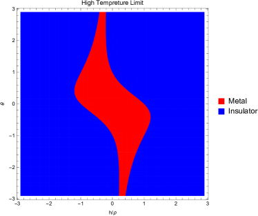
(a) The red region indicates metallic behavior. The blue region indicates insulating behavior.

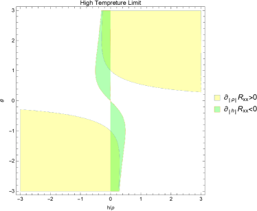
(b) Yellow region indicates Mott-like behavior. Green Region indicates negative magneto-resistance.

Figure 1: Parameter space in terms of $\theta$ and $h/\rho$ in the high temperature limit. Note that $\theta\equiv\mathcal{L}^{\left(0,1\right)}\left(0,0\right)$.

Finally, we consider the high temperature limit $T\gg\left(\sqrt{h}\text{, }\sqrt{\rho}\text{, }\alpha\right)$. In this limit, eqn. $\left(\ref{eq:HT}\right)$ gives

$$T\approx\frac{3}{4\pi}r_{h}.$$ (38)

The resistance then reduces to

$$R_{xx}=\frac{1}{1+\theta^{2}}\left\{1+\frac{9}{16\pi^{2}\alpha^{2}T^{2}}\left[\left(1+\theta^{2}\right)h^{2}+2\theta\rho h-\frac{1-\theta^{2}}{1+\theta^{2}}\rho^{2}\right]\right\}+\mathcal{O}\left(T^{-4}\right)\text{,}$$ (39)

which only depends on $\theta=\mathcal{L}^{\left(0,1\right)}\left(0,0\right)$ and is independent of the nonlinear effects of the NLED field. This is understood as the nonlinear terms being suppressed by the high temperature. One can define a metal and an insulator for $dR_{xx}/dT>0$ and $dR_{xx}/dT<0$, respectively. Eqn. $\left(\ref{eq:Rxx}\right)$ shows that, for any NLED model in the high temperature, a metal-insulator transition (MIT) occurs when the term $\left(1+\theta^{2}\right)h^{2}+2\theta\rho h-\frac{1-\theta^{2}}{1+\theta^{2}}\rho^{2}$ changes the sign. In FIG. 1(a), we plot the parameter space for a metal and an insulator with respect to $h/\rho$ and $\theta$. Note that, if $\theta\neq 0$, there is no $\left(\rho,h\right)\rightarrow\left(\rho,-h\right)$ or $\left(\rho,h\right)\rightarrow\left(-\rho,h\right)$ symmetries for $\sigma_{ij}$ or $R_{ij}$. However, $\sigma_{ij}$ or $R_{ij}$ are invariant under $\left(\rho,h\right)\rightarrow\left(-\rho,-h\right)$. The parameter space for $\partial_{\left|\rho\right|}R_{xx}$ and $\partial_{\left|h\right|}R_{xx}$ are plotted in FIG. 1(b), where we find

• Green Region: In this region, one has that $\partial R_{xx}/\partial\left|h\right|<0$. To describe how the electrical resistance responds to an externally-applied magnetic field, one can define magneto-resistance as

  $$MR=\frac{R_{xx}\left(h\right)-R_{xx}\left(0\right)}{R_{xx}\left(0\right)}\text{.}$$ (40)

  So the green region has negative magneto-resistance at given temperature and charge density.

• Yellow Region: In this region, one has that $\partial R_{xx}/\partial\left|\rho\right|>0$. This is Mott-like behavior, which can be explained by the electronic traffic jam: strong enough $e$-$e$ interactions prevent the available mobile charge carriers to efficiently transport charges. In particular, when $h=0$, eqn. $\left(\ref{eq:Rxx}\right)$ gives that $\partial R_{xx}/\partial\left|\rho\right|>0$ as long as $\theta^{2}>1$.

If the NLED Lagrangian $\mathcal{L}\left(s,p\right)$ is CP invariant, one has $\theta=0$. In this case, $R_{xx}$ becomes

$$R_{xx}=1+\frac{9\left(h^{2}-\rho^{2}\right)}{16\pi^{2}\alpha^{2}T^{2}}+\mathcal{O}\left(T^{-4}\right)\text{,}$$ (41)

which gives that the system displays metallic behavior for $\left|h/\rho\right|<1$ and insulating behavior for $\left|h/\rho\right|>1$. Moreover, one always has that $\partial R_{xx}/\partial\left|h\right|>0$ and $\partial R_{xx}/\partial\left|\rho\right|<0$. Therefore, there is no negative magneto-resistance or Mott-like behavior for CP invariant NLED models in the high temperature limit. Note that, in IN-Cremonini:2017qwq , eqn. $\left(\ref{eq:Rxxtheta=0}\right)$ was also obtained for the high temperature limit of the DBI model.

IV Examples

In this section, we will use eqns. $\left(\ref{eq:HT}\right)$, $\left(\ref{eq:rho}\right)$ and $\left(\ref{eq:DCconductity}\right)$ to study the dependence of the in-plane resistance $R_{xx}$ on the temperature $T$, the charge density $\rho$ and the magnetic field $h$ in Maxwell, Maxwell-Chern-Simons, Born-Infeld, square and logarithmic electrodynamics. The behavior of $R_{xx}$ in the high temperature limit has already been discussed in section III. So we will focus on the behavior of $R_{xx}$ around $T=0$ in this section.

IV.1 Maxwell Electrodynamics

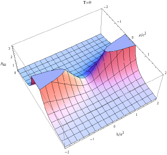
(a) $T=0$.

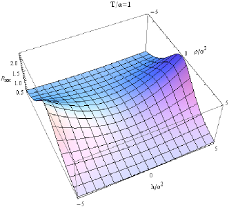
(b) $T/\alpha=1$.

Figure 2: The resistance $R_{xx}$ versus $\rho/a^{2}$ and $h/a^{2}$ at $T=0$ and $T/\alpha=1$ for Maxwell electrodynamics.

To study the effects of the nonlinear and $\theta$ terms on $R_{xx}$, we first consider Maxwell electrodynamics, in which $\mathcal{L}\left(s,p\right)=s$. At $T=0$, the resistance $R_{xx}$ is given by

$$R_{xx}=\frac{\sqrt{1+12\left(h^{2}/\alpha^{4}+\rho^{2}/\alpha^{4}\right)}}{1+12\rho^{2}/\alpha^{4}},$$ (42)

which is plotted against $\rho/\alpha^{2}$ and $h/\alpha^{2}$ in FIG. 2(a). At $T/\alpha=1$, we also plot $R_{xx}$ against $\rho/\alpha^{2}$ and $h/\alpha^{2}$ in FIG. 2(b). Both figures show the saddle surfaces, which imply that $\partial R_{xx}/\partial\left|h\right|>0$ and $\partial R_{xx}/\partial\left|\rho\right|<0$. So for Maxwell electrodynamics, $R_{xx}$ does not possess negative magneto-resistance or Mott-like behavior.

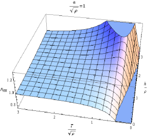
(a) Plot of $R_{xx}$ against $h/\rho$ and $T/\sqrt{\rho}$ for $\alpha/\sqrt{\rho}=1$.

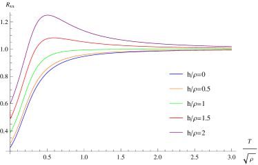
(b) Plot of $R_{xx}$ against $T/\sqrt{\rho}$ for various values of $h/\rho$ for $\alpha/\sqrt{\rho}=1$.

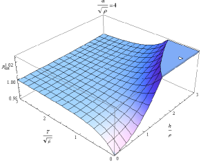
(c) Plot of $R_{xx}$ against $h/\rho$ and $T/\sqrt{\rho}$ for $\alpha/\sqrt{\rho}=4$.

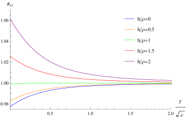
(d) Plot of $R_{xx}$ against $T/\sqrt{\rho}$ for various values of $h/\rho$ for $\alpha/\sqrt{\rho}=4$.

Figure 3: Plots of $R_{xx}$ with $\alpha/\sqrt{\rho}=1$ and $\alpha/\sqrt{\rho}=4$ for Maxwell electrodynamics.

In FIG. 3, we display the dependence of $R_{xx}$ on $h/\rho$ and $T/\sqrt{\rho}$ for $\alpha/\sqrt{\rho}=1$ and $\alpha/\sqrt{\rho}=4$, respectively. For $h<\rho$, FIG. 3 shows that the temperature dependence of $R_{xx}$ is similar in both $\alpha/\sqrt{\rho}=1$ and $\alpha/\sqrt{\rho}=4$ cases. The resistance $R_{xx}$ increases monotonically as the temperature increasing, which corresponds to metallic behavior. For $h>\rho$, the $\alpha/\sqrt{\rho}=1$ and $\alpha/\sqrt{\rho}=4$ cases show different temperature dependence of $R_{xx}$. When $\alpha/\sqrt{\rho}=1$, FIGs. 3(a) and 3(b) show that, as the temperature increases, $R_{xx}$ increases first and then decreases monotonically after reaching a maximum. The insulating behavior appears at high temperatures in this case. When $\alpha/\sqrt{\rho}=4$, FIGs. 3(c) and 3(d) show that $R_{xx}$ decreases monotonically as one increases the temperature, which corresponds to insulating behavior. So in the $\alpha/\sqrt{\rho}=4$ and $\alpha/\sqrt{\rho}=1$ cases at high temperatures, increasing the magnetic field would induce a finite-temperature transition or crossover from metallic to insulating behavior.

IV.2 Maxwell-Chern-Simons Electrodynamics

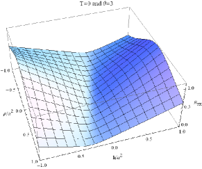
(a) Plot of $R_{xx}$ against $h/\alpha^{2}$ and $\rho/\alpha^{2}$ for $\theta=3$.

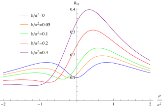
(b) Plot of $R_{xx}$ against $\rho/\alpha^{2}$ for various values of $h/\alpha^{2}$ for $\theta=3$.

Figure 4: Plots of $R_{xx}$ with $\theta=3$ at $T=0$ for Maxwell-Chern-Simons electrodynamics.

The Lorentz and gauge invariance allow the electrodynamics Lagrangian to have a CP-violating $\theta$ term

$$\mathcal{L}\left(s,p\right)=s+\theta p\text{.}$$ (43)

We now discuss the dependence of $R_{xx}$ on $\rho$ and $h$ at $T=0$. The resistance $R_{xx}$ can be expressed in terms of $r_{h}$, $\rho$ and $h$:

$$R_{xx}=\frac{\alpha^{2}r_{h}^{2}\left[\left(1+\theta^{2}\right)h^{2}+\alpha^{2}r_{h}^{2}+2\theta h\rho+\rho^{2}\right]}{\left(1+\theta^{2}\right)\alpha^{4}r_{h}^{4}+h^{2}\rho^{2}+2\alpha^{2}r_{h}^{2}\rho^{2}+\rho^{2}\left(\rho+\theta h\right)^{2}}.$$ (44)

At zero temperature, the resistance $R_{xx}$ becomes

$$R_{xx}=\frac{\sqrt{1+12\left[h^{2}/\alpha^{4}+\left(\rho/\alpha^{2}+\theta h^{2}/\alpha^{2}\right)^{2}\right]}}{1+\theta^{2}+12\rho^{2}/\alpha^{4}}.$$ (45)

In FIG. 4(a), we plot $R_{xx}$ versus $\rho/\alpha^{2}$ and $h^{2}/\alpha^{2}$ with $\theta=3$. Similar to Maxwell electrodynamics, we have a saddle surface. However, the valley in FIG. 4(a) is at $\rho/\alpha^{2}+3h^{2}/\alpha^{2}=0$, instead of $\rho/\alpha^{2}=0$. This twist of the valley would result in the appearance of negative magneto-resistance and Mott-like behavior.

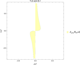
(a) $\theta=1$.

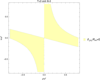
(b) $\theta=3$.

Figure 5: Parameter space for $\partial_{\left|\rho\right|}R_{xx}>0$ in terms of $\rho/\alpha^{2}$ and $h/\alpha^{2}$ with $\theta=1$ and $\theta=3$ at $T=0$ for Maxwell-Chern-Simons electrodynamics.

The dependence of $R_{xx}$ on $h$ can be obtained by computing $\partial_{h}R_{xx}$. We find that solving $\partial_{\left|h\right|}R_{xx}<0$ gives

$$-\frac{\theta}{1+\theta^{2}}<h/\rho<0\text{ for }\theta>0\text{, and }0<h/\rho<-\frac{\theta}{1+\theta^{2}}\text{ for }\theta<0\text{,}$$ (46)

where one has negative magneto-resistance. Note that, in the high temperature limit, $\partial_{\left|h\right|}R_{xx}<0$ reduces to

$$-\frac{2\theta}{1+\theta^{2}}<h/\rho<0\text{ for }\theta>0\text{, and }0<h/\rho<-\frac{2\theta}{1+\theta^{2}}\text{ for }\theta<0\text{.}$$ (47)

When $h=0$, we find that

$$\partial_{\left|\rho\right|}R_{xx}>0\Rightarrow\rho^{2}<\left(\frac{\theta^{2}-1}{12}\right)\alpha^{4}\text{,}$$ (48)

which means that there is no Mott-like behavior for $h=0$ if $\theta^{2}\leq 1$. In FIG. 5, we plot the parameter space for $\partial_{\left|\rho\right|}R_{xx}>0$ in terms of $\rho/\alpha^{2}$ and $h/\alpha^{2}$ with $\theta=1$ and $\theta=3$. In the yellow region, one has $\partial_{\left|\rho\right|}R_{xx}>0$. As expected, the line $h=0$ is in the yellow region for $\theta=3$ while it is not for $\theta=1$. In FIG. 4(b), we plot $R_{xx}$ versus $\rho/\alpha^{2}$ for various values of $h/\alpha^{2}$. One has $h/\alpha^{2}=0$ for the blue line, and it has a minimum at $\rho/\alpha^{2}=0$. As one increases the magnitude of the charge density, the value of $R_{xx}$ first increases, then reaches a maximum, and then decreases monotonically. For $h/\alpha^{2}\neq 0$, the behavior of $R_{xx}$ is different when one moves along the positive and negative $\rho/\alpha^{2}$ directions. Along the positive $\rho/\alpha^{2}$ direction, the behavior of $R_{xx}$ is similar to the $h/\alpha^{2}=0$ case. However, if one increases the magnitude of the charge density along the negative $\rho/\alpha^{2}$ direction, the value of $R_{xx}$ first decreases until reaching a minimum, then increases until reaching a maximum, and then decreases monotonically.

IV.3 Born-Infeld Electrodynamics

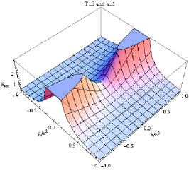
(a) $a=1.$

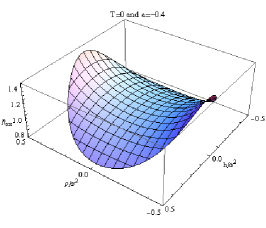
(b) $a=-0.4.$

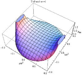
(c) $a=-1.$

Figure 6: Plots of $R_{xx}$ versus $\rho/\alpha^{2}$ and $h/\alpha^{2}$ with $a=1$, $a=-0.4$ and $a=-1$ at $T=0$ for Born-Infeld electrodynamics.

Born-Infeld electrodynamics is described by the Lagrangian density

$$\mathcal{L}\left(s,p\right)=\frac{1}{a}\left(1-\sqrt{1-2as-a^{2}p^{2}}\right)\text{,}$$ (49)

where the coupling parameter $a$ is related to the string tension $\alpha^{\prime}$ as $a=\left(2\pi\alpha^{\prime}\right)^{2}$. When $\left|a\right|\ll 1$, we can recover the Maxwell Lagrangian. For the $a>0$ case, the properties of the resistance $R_{xx}$ were discussed in IN-Cremonini:2017qwq . It showed that the behavior of $R_{xx}$ obtained in IN-Cremonini:2017qwq was quite similar to that in the Maxwell case, which has been investigated in section IV.1. In fact, there is no appearance of negative magneto-resistance or Mott-like behavior at low temperatures, maybe for all the temperatures, in both cases. To illustrate this point, we plot $R_{xx}$ versus $\rho/\alpha^{2}$ and $h^{2}/\alpha^{2}$ at $T=0$ for Born-Infeld electrodynamics with $a=1$ in FIG. 6(a), which shows that $\partial_{\left|\rho\right|}R_{xx}<0$ and $\partial_{\left|h\right|}R_{xx}>0$. Note that FIGs. 2(a) and 6(a) look alike. Moreover, both cases have quite similar behavior of $R_{xx}$ as a function of $h/\rho$ and $T/\sqrt{\rho}$ for the small and large values of the momentum dissipation parameter.

On the other hand, the $a<0$ case turns out more interesting. For the case with vanishing magnetic filed, the properties of $\sigma_{xx}$ have been analyzed in depth in IN-Baggioli:2016oju , in which it showed that the conductivity could decrease with increasing charge density for large enough self-interaction strength${}^{\left[\ref{ft:1}\right]}$. Here, we extend the analysis to the non-vanishing magnetic field case. We can solve eqn. $\left(\ref{eq:Grt}\right)$ for $A_{t}^{\prime}\left(r\right)$:

$$A_{t}^{\prime}\left(r\right)=\frac{\rho}{\sqrt{r^{4}+a\left(h^{2}+\rho^{2}\right)}},$$ (50)

which shows that there is a singularity at $r=r_{s}\equiv\sqrt[1/4]{-a\left(h^{2}+\rho^{2}\right)}$ for $a<0$. To have a physical solution, we need to hide the singularity behind the horizon: $r_{s}<r_{h}$, which could put an upper bound on $h^{2}+\rho^{2}$.

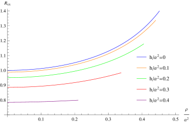
(a) Plot of $R_{xx}$ against $\rho/\alpha^{2}$ with $a=-0.4$ at $T=0$ for various values of $h/\alpha^{2}$.

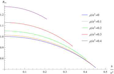
(b) Plot of $R_{xx}$ against $h/\alpha^{2}$ with $a=-0.4$ at $T=0$ for various values of $\rho/\alpha^{2}$.

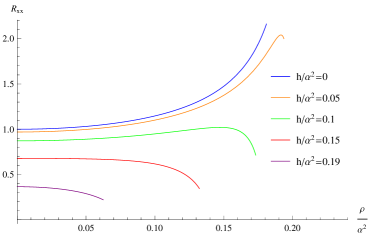
(c) Plot of $R_{xx}$ against $\rho/\alpha^{2}$ with $a=-1$ at $T=0$ for various values of $h/\alpha^{2}$.

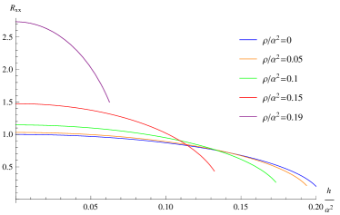
(d) Plot of $R_{xx}$ against $h/\alpha^{2}$ with $a=-1$ at $T=0$ for various values of $\rho/\alpha^{2}$.

Figure 7: Plots of $R_{xx}$ against the charge density $\rho$ and the magnetic field $h$ with $a=-0.4$ and $a=-1$ at $T=0$ for Born-Infeld electrodynamics.

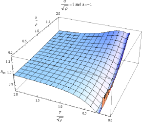
(a) Plot of $R_{xx}$ against $h/\rho$ and $T/\sqrt{\rho}$ for $\alpha/\sqrt{\rho}=1$.

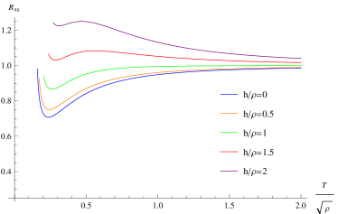
(b) Plot of $R_{xx}$ against $T/\sqrt{\rho}$ for various values of $h/\rho$ for $\alpha/\sqrt{\rho}=1$.

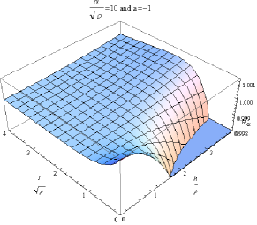
(c) Plot of $R_{xx}$ against $h/\rho$ and $T/\sqrt{\rho}$ for $\alpha/\sqrt{\rho}=10$.

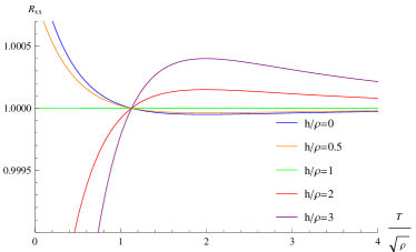
(d) Plot of $R_{xx}$ against $T/\sqrt{\rho}$ for various values of $h/\rho$ for $\alpha/\sqrt{\rho}=10$.

Figure 8: Plots of the temperature dependence of $R_{xx}$ with $\alpha/\sqrt{\rho}=1$ and $\alpha/\sqrt{\rho}=10$ at finite charge density for Born-Infeld electrodynamics with $a=-1$.

We first discuss behavior of $R_{xx}$ at $T=0$. At zero temperature, the condition $r_{s}<r_{h}$ gives that there is an upper bound on $h^{2}+\rho^{2}$ for $a<-\frac{1}{6}$:

$$\frac{h^{2}+\rho^{2}}{\alpha^{4}}\leq\frac{-a}{\left(1+6a\right)^{2}}.$$ (51)

We plot $R_{xx}$ versus $\rho/\alpha^{2}$ and $h^{2}/\alpha^{2}$ at $T=0$ with $a=-0.4$ and $a=-1$ in FIGs. 6(b) and 6(c), respectively. It is noteworthy that, in FIGs. 6(b) and 6(c), the domains of $R_{xx}$ are bounded by eqn. $\left(\ref{eq:upperbound}\right)$. In FIGs. 7(b) and 7(d), we display how the resistance $R_{xx}$ depends $h/\alpha^{2}$ for various values of $\rho/\alpha^{2}$ in the $a=-0.4$ and $a=-1$ cases, respectively. In both cases, $R_{xx}$ decreases monotonically with increasing the magnitude of the magnetic field at constant charge density, which shows that the system exhibits negative magneto-resistance in all of the allowed parameter range. The resistance $R_{xx}$ as a function of $\rho/\alpha^{2}$ for different values of $h/\alpha^{2}$ in the $a=-0.4$ case is presented in FIG. 7(a). We find that $R_{xx}$ increases monotonically as one increases the magnitude of the charge density with the magnetic field fixed, which shows that Mott-like behavior occurs in all of the allowed parameter range. We also display the resistance $R_{xx}$ for $a=-1$ in FIG. 7(c). When $h=0$, $R_{xx}$ increases monotonically with increasing the magnitude of the charge density. For a small but non-vanishing $h/\alpha^{2}$, e.g. $h/\alpha^{2}=0.05$ and $0.1$, the non-monotonic behavior at large values of $\rho/\alpha^{2}$ appears. As the value of $\rho/\alpha^{2}$ increases, $R_{xx}$ increases first and then decreases after reaching a maximum. However for a larger value of $h/\alpha^{2}$, e.g. $h/\alpha^{2}=0.15$ and $0.19$, we find that $R_{xx}$ decreases monotonically with increasing the magnitude of the charge density, and hence Mott-like behavior disappears. In summary, Mott-like behavior always occurs in the $a=-0.4$ case. However in the $a=-1$ case, Mott-like behavior appears for a weak magnetic field, and a strong enough magnetic field could destroy it.

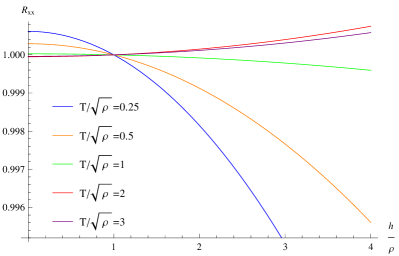
(a) Plot of $R_{xx}$ against $h/\rho$ at finite charge density with $\alpha/\sqrt{\rho}=10$ for various values of $T/\sqrt{\rho}$.

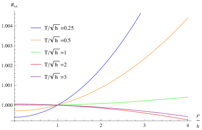
(b) Plot of $R_{xx}$ against $\rho/h$ at finite magnetic field with $\alpha/\sqrt{h}=10$ for various values of $T/\sqrt{h}$.

Figure 9: Plots of how the dependences of $R_{xx}$ on $\rho$ and $h$ change with respect to $T$. Here we consider Born-Infeld electrodynamics with $a=-1$.

Next, we consider the temperature dependence of $R_{xx}$ at finite charge density. Focusing on the $a=-1$ case, we present how $R_{xx}$ depends on $h/\rho$ and $T/\sqrt{\rho}$ for $\alpha/\sqrt{\rho}=1$ and $\alpha/\sqrt{\rho}=10$ in FIG. 8. At zero temperature, eqn. $\left(\ref{eq:upperbound}\right)$ would put an upper bound on the value of $h/\rho$

$$\left(h/\rho\right)^{2}\leq\frac{\left(\alpha/\sqrt{\rho}\right)^{4}}{25}-1.$$ (52)

When $\alpha/\sqrt{\rho}=1$, the RHS of the above equation is negative, which explains why the curves in FIG. 8(b) could not go to zero temperature. Since Born-Infeld electrodynamics is CP invariant, one has insulating behavior for $h/\rho>1$ and metallic behavior for $h/\rho<1$ in the high temperature limit, which is clearly shown in FIGs. 8(b) and 8(d). However, at low temperatures, the temperature dependence of $R_{xx}$ in the $a<0$ case is quite different from those in the $a>0$ and Maxwell cases. For $\alpha/\sqrt{\rho}=1$, FIG. 8(b) displays insulating behavior at low temperatures. As one increases the temperature, the system would start to exhibit metallic behavior. If one keeps increasing the temperature, the system would stay metallic behavior for $h/\rho<1$, but it would return to insulating behavior for $h/\rho<1$. In the $\alpha/\sqrt{\rho}=10$ case, according to FIG. 8(d), one has insulating behavior for $h/\rho<1$ and metallic behavior for $h/\rho>1$ at low temperatures. Therefore, increasing the magnitude of the magnetic field would induce a transition or crossover from insulating to metallic behavior at low temperatures and that from metallic to insulating behavior at high temperatures.

We find that the system does not exhibit negative magneto-resistance or Mott-like behavior at high temperatures. If one has negative magneto-resistance or Mott-like behavior at low temperatures, they would disappear at a high enough temperature. We plot $R_{xx}$ as a function of $h/\rho$ for various values of $T/\sqrt{\rho}$ with $\alpha/\sqrt{\rho}=10$ in FIG. 9(a). With a fixed value of the charge density, FIG. 9(a) shows that $R_{xx}$ decreases with increasing $h$ for $T/\sqrt{\rho}=0.25$, $0.5$ and $1$, and $R_{xx}$ increases with increasing $h$ for $T/\sqrt{\rho}=2$ and $3$. Similarly, FIG. 9(b) shows that, with a fixed value of the magnetic field, the system displays Mott-like behavior for $T/\sqrt{h}=0.25$, $0.5$ and $1$, and $R_{xx}$ decreases with increasing $\rho$ for $T/\sqrt{h}=2$ and $3$.

IV.4 Square Electrodynamics

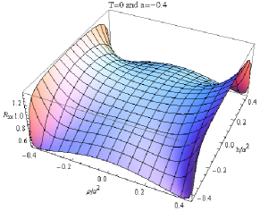
(a) Plot of $R_{xx}$ against $h/\alpha^{2}$ and $\rho/\alpha^{2}$ at $T=0$ with $a=-0.4$.

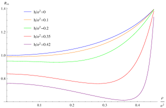
(b) Plot of $R_{xx}$ against $\rho/\alpha^{2}$ for various values of $h/\alpha^{2}$ at $T=0$ with $a=-0.4$.

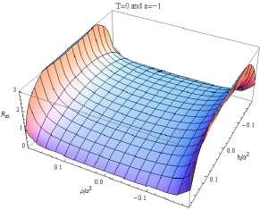
(c) Plot of $R_{xx}$ against $h/\alpha^{2}$ and $\rho/\alpha^{2}$ at $T=0$ with $a=-1$.

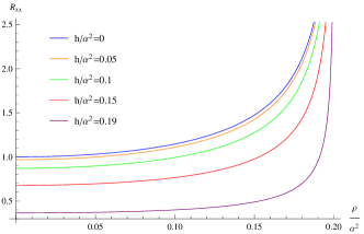
(d) Plot of $R_{xx}$ against $\rho/\alpha^{2}$ for various values of $h/\alpha^{2}$ at $T=0$ with $a=-1$.

Figure 10: Plots of $R_{xx}$ at $T=0$ for square electrodynamics. Top figures: $a=-0.4$. Bottom figures: $a=-1$.

Consider a Born–Infeld like Lagrangian

$$\mathcal{L}\left(s,p\right)=\frac{1}{a}\left(1-\sqrt{1-2as}\right)\text{,}$$ (53)

which gives the same result for $\sigma_{ij}/R_{ij}$ as Born-Infeld electrodynamics in the $h=0$ case. We now study the dependence of $R_{xx}$ on $\rho$ and $h$ at $T=0$. Since the behavior of $R_{xx}$ in the $a>0$ case is similar to that in Maxwell electrodynamics, we focus on the $a<0$ case. In FIG. 10(a), we plot $R_{xx}$ as a function of $\rho/\alpha^{2}$ and $h^{2}/\alpha^{2}$ with $a=-0.4$, which displays negative magneto-resistance at fixed charge density for all of the allowed parameter range. FIG. 10(b) shows the dependence of $R_{xx}$ on $\rho/\alpha^{2}$ for various values of $h^{2}/\alpha^{2}$. For a small value of $h/\alpha^{2}$, e.g. $h/\alpha^{2}=0$ and $0.1$, $R_{xx}$ increases monotonically with increasing $\rho/\alpha^{2}$. However for a larger value of $h/\alpha^{2}$, e.g. $h/\alpha^{2}=0.2$, $0.35$ and $0.42$, $R_{xx}$ first decreases, then reaches a minimum, and then increases monotonically with increasing $\rho/\alpha^{2}$. In this case, Mott-like behavior would appear for large enough values of $\rho/\alpha^{2}$. On the other hand, according to FIGs. 10(c) and 10(d), the system exhibits negative magneto-resistance and Mott-like behavior for all of the allowed parameter range in the $a=-1$ case.

IV.5 Logarithmic Electrodynamics

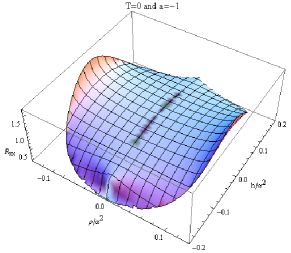
(a) Plot of $R_{xx}$ against $h/\alpha^{2}$ and $\rho/\alpha^{2}$ at $T=0$ with $a=-1$.

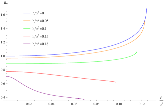
(b) Plot of $R_{xx}$ against $\rho/\alpha^{2}$ for various values of $h/\alpha^{2}$ at $T=0$ with $a=-1$.

Figure 11: Plots of $R_{xx}$ at $T=0$ for logarithmic electrodynamics with $a=-1$.

Finally, we consider logarithmic electrodynamics, whose Lagrangian is described by

$$\mathcal{L}\left(s,p\right)=-\frac{1}{a}\log\left(1-as-\frac{a^{2}p^{2}}{2}\right).$$ (54)

We display the dependence of $R_{xx}$ on $\rho/\alpha^{2}$ and $h/\alpha^{2}$ in the the $a=-1$ case at $T=0$ in FIG. 11(a), which shows that $\partial R_{xx}/\partial\left|h\right|<0$. However, FIG 11(b) shows that $\partial R_{xx}/\partial\left|\rho\right|>0$ for small values of $h/\alpha^{2}$, and $\partial R_{xx}/\partial\left|\rho\right|<0$ for large enough values of $h/\alpha^{2}$, which means a strong enough magnetic field would destroy Mott-like behavior.

V Discussion and Conclusion

	Lagrangian	Parameter	$\rho$ dependence of $R_{xx}$	$h$ dependence of $R_{xx}$
Maxwell	$s$		$\partial_{\left|\rho\right|}R_{xx}<0$. See FIG. 2(a).	$\partial_{\left|h\right|}R_{xx}>0$. See FIG. 2(a).
Maxwell-Chern-Simons	$s+\theta p$	$\theta\neq 0$	There exists parameter space region for $\partial_{\left|\rho\right|}R_{xx}>0$. See FIG. 5.	There exists parameter space region for $\partial_{\left|h\right|}R_{xx}<0$. See eqn. $\left(\ref{eq:csnm}\right).$
		$a>0$	$\partial_{\left|\rho\right|}R_{xx}<0$. See FIG. 6(a).	$\partial_{\left|h\right|}R_{xx}>0$. See FIG. 6(a).
Born-Infeld	$\frac{1-\sqrt{1-2as-a^{2}p^{2}}}{a}$	$a=-0.4$	$\partial_{\left|\rho\right|}R_{xx}>0$. See FIG. 7(a).	$\partial_{\left|h\right|}R_{xx}<0$. See FIG. 7(b).
		$a=-1$	$\partial_{\left|\rho\right|}R_{xx}>0$ for small values of $h/\alpha^{2}$ and $\rho/\alpha^{2}$. See FIG. 7(c).	$\partial_{\left|h\right|}R_{xx}<0$. See FIG. 7(d).
		$a>0$	$\partial_{\left|\rho\right|}R_{xx}<0$.	$\partial_{\left|h\right|}R_{xx}>0.$
Square	$\frac{1-\sqrt{1-2as}}{a}$	$a=-0.4$	$\partial_{\left|\rho\right|}R_{xx}>0$ for small values of $h/\alpha^{2}$. For larger values of $h/\alpha^{2}$, $\partial_{\left|\rho\right|}R_{xx}>0$ only for large enough values of $\rho/\alpha^{2}$. See FIG. 10(b).	$\partial_{\left|h\right|}R_{xx}<0$. See FIG. 10(a).
		$a=-1$	$\partial_{\left|\rho\right|}R_{xx}>0$.  See FIG. 10(d).	$\partial_{\left|h\right|}R_{xx}<0$. See FIG. 10(c).
		$a>0$	$\partial_{\left|\rho\right|}R_{xx}<0.$	$\partial_{\left|h\right|}R_{xx}>0.$
Logarithmic	$\frac{-\log\left(1-as-\frac{a^{2}p^{2}}{2}\right)}{a}$	$a=-1$	$\partial_{\left|\rho\right|}R_{xx}>0$ for small values of $h/\alpha^{2}$. See FIG. 11(b).	$\partial_{\left|h\right|}R_{xx}<0$. See FIG. 11(a).

Table 1: The dependence of the in-plane resistance $R_{xx}$ on $\rho/\alpha^{2}$ and $h/\alpha^{2}$ at $T=0$. Here $\alpha$ is a parameter responsible for generating momentum dissipation. Note that $\partial_{\left|h\right|}R_{xx}<0$ means negative magneto-resistance while $\partial_{\left|\rho\right|}R_{xx}<0$ means Mott-like behavior.

In this paper, we used gauge/gravity duality to investigate the properties of the DC conductivities with a finite magnetic field of a strongly correlated system in $2+1$ dimensions. The charge current in the boundary field theory is dual to a NLED field in bulk. In our holographic setup, we considered the backreaction effects of the NLED field on the geometry and introduced axionic scalars to generate momentum dissipation. We then presented the expressions for the DC conductivities for a general NLED field. Specifically, one can use eqns. $\left(\ref{eq:HT}\right)$, $\left(\ref{eq:rho}\right)$ and $\left(\ref{eq:DCconductity}\right)$ to express the DC conductivities in terms of the temperature $T$, the charge density $\rho$ and the magnetic field $h$ of the dual field theory. In the second part of our paper, we discussed the properties of the in-plane resistance $R_{xx}$ in some interesting NLED models, where there appeared Mott-like behavior or negative magneto-resistance in some cases. In Table 1, we summarize the results for the $\rho$ and $h$ dependences of $R_{xx}$ at zero temperature in the NLED models discussed above.

Table 1 shows that the behavior of $R_{xx}$ as a function of $\rho$ and $h$ is sensitive to the sign of the parameter $a$. To shed light on the role of $a$, we calculate the correction to the coulomb force between two electrons due to non-linearities from the NLED Lagrangian $\mathcal{L}\left(s,p\right)$. The corrected coulomb force is given by

$$F\approx\frac{e^{2}}{4\pi r^{2}}\left[1-\frac{\mathcal{L}^{\left(2,0\right)}\left(0,0\right)}{2}\left(\frac{e}{4\pi r^{2}}\right)^{2}\right].$$ (55)

For the NLED models discussed in section IV, we have $\mathcal{L}^{\left(2,0\right)}\left(0,0\right)=a$. For $a>0$, the non-linearities correction tends to reduce the strength of the repulsive force between two electrons. However for $a<0$, the correction tends to increase the strength of the force. So it is natural to expect that a negative $a$ may correspond to strong interactions between electrons in our holographic model, which could lead to Mott-like behavior ${}^{\left[\ref{ft:2}\right]}$.

It is interesting to note that Born-Infeld electrodynamics with $a=-1$ could describe Mott insulator to metal transition (IMT) induced by a magnetic field. In fact, FIG. 8(d) shows that, at low temperatures, the system has insulating/metallic behavior for a weak/strong magnetic field. On the other hand, FIG. 7(c) displays that, for a weak magnetic field at low temperatures, the system usually has Mott-like behavior and hence is a Mott-Insulator. When the magnetic field grows strong enough, Mott-like behavior disappears, and meanwhile, the system exhibits metallic behavior. A magnetic field-induced IMT for a Mott system, namely a bilayer ruthenate, Ti-doped Ca₃Ru₂O₇, was presented in CON-Zhu2016 . Our analysis for IMT is rather qualitative, and it deserves future more detailed studies.

For a negative enough $a$, we found that, at low temperatures, the resistance $R_{xx}$ always decreases with increasing magnetic field, which appears as negative magneto-resistance. On the other hand, the behavior of $R_{xx}$ in the $a>0$ NLED models is similar to that in Maxwell electrodynamics, in which one always have positive-resistance. It seems that, decreasing $a$ from a positive value to a negative one, which corresponds to increasing the strength of the interactions between electrons, would lead the magneto-resistance to change from positive to negative. It showed in CON-Zhou2011 that the magneto-resistance could change from positive to negative by gradually introducing artificial disorder through Ga⁺ ion irradiation to pristine graphene. To relate our results to the experiments, we need to better understand how $a$ is related to external control parameters.

In this paper, we found the $\sigma_{ij}/R_{ij}$ expressions for a general NLED field. Our analyses for the properties of the resistance in NLED models are preliminary. One can use these expressions to find or construct a NLED model to realize some interesting experimental results, such as the scaling relationship between applied magnetic field and temperature observed in the magneto-resistance of the pnictide superconductor.

- (1) T. Banks, W. Fischler, S. H. Shenker and L. Susskind, “M theory as a matrix model: A Conjecture,” Phys. Rev. D 55, 5112 (1997) doi:10.1103/PhysRevD.55.5112 [hep-th/9610043].
- (2) J. M. Maldacena, “The Large N limit of superconformal field theories and supergravity,” Int. J. Theor. Phys. 38, 1113 (1999) [Adv. Theor. Math. Phys. 2, 231 (1998)] doi:10.1023/A:1026654312961 [hep-th/9711200].
- (3) E. Witten, “Anti-de Sitter space and holography,” Adv. Theor. Math. Phys. 2, 253 (1998) doi:10.4310/ATMP.1998.v2.n2.a2 [hep-th/9802150].
- (4) S. S. Gubser, “Breaking an Abelian gauge symmetry near a black hole horizon,” Phys. Rev. D 78, 065034 (2008) doi:10.1103/PhysRevD.78.065034 [arXiv:0801.2977 [hep-th]].
- (5) S. A. Hartnoll, C. P. Herzog and G. T. Horowitz, “Building a Holographic Superconductor,” Phys. Rev. Lett. 101, 031601 (2008) doi:10.1103/PhysRevLett.101.031601 [arXiv:0803.3295 [hep-th]].
- (6) S. S. Lee, “A Non-Fermi Liquid from a Charged Black Hole: A Critical Fermi Ball,” Phys. Rev. D 79, 086006 (2009) doi:10.1103/PhysRevD.79.086006 [arXiv:0809.3402 [hep-th]].
- (7) H. Liu, J. McGreevy and D. Vegh, “Non-Fermi liquids from holography,” Phys. Rev. D 83, 065029 (2011) doi:10.1103/PhysRevD.83.065029 [arXiv:0903.2477 [hep-th]].
- (8) M. Cubrovic, J. Zaanen and K. Schalm, “String Theory, Quantum Phase Transitions and the Emergent Fermi-Liquid,” Science 325, 439 (2009) doi:10.1126/science.1174962 [arXiv:0904.1993 [hep-th]].
- (9) G. H. Wannier, “Theorem on the Magnetoconductivity of Metals,” Phys. Rev. B 5, 3836 (1972).
- (10) H. Negishi, H. Yamada, K. Yuri, M. Sasaki and M. Inoue “Negative magnetoresistance in crystals of the paramagnetic intercalation compound MnxTiS2,” Phys. Rev. B 56, 11144 (1997).
- (11) C. Z. Li et al, “Giant negative magnetoresistance induced by the chiral anomaly in individual Cd3As2 nanowires,” Nature Communications 6, 10137 (2015), [arXiv:1504.07398 [cond-mat.str-el]].
- (12) H.-J. Kim, K.-S. Kim, J. F. Wang, M. Sasaki, N. Satoh, A. Ohnishi, M. Kitaura, M. Yang, and L. Li, “Dirac vs. Weyl in topological insulators: Adler-BellJackiw anomaly in transport phenomena,” Phys. Rev. Lett. 111, 246603 (2013), [arXiv:1307.6990 [cond-mat.str-el]].
- (13) A. Jimenez-Alba, K. Landsteiner and L. Melgar, “Anomalous magnetoresponse and the Stückelberg axion in holography,” Phys. Rev. D 90, 126004 (2014) doi:10.1103/PhysRevD.90.126004 [arXiv:1407.8162 [hep-th]].
- (14) A. Jimenez-Alba, K. Landsteiner, Y. Liu and Y. W. Sun, “Anomalous magnetoconductivity and relaxation times in holography,” JHEP 1507, 117 (2015) doi:10.1007/JHEP07(2015)117 [arXiv:1504.06566 [hep-th]].
- (15) K. Landsteiner, Y. Liu and Y. W. Sun, “Negative magnetoresistivity in chiral fluids and holography,” JHEP 1503, 127 (2015) doi:10.1007/JHEP03(2015)127 [arXiv:1410.6399 [hep-th]].
- (16) Y. W. Sun and Q. Yang, “Negative magnetoresistivity in holography,” JHEP 1609, 122 (2016) doi:10.1007/JHEP09(2016)122 [arXiv:1603.02624 [hep-th]].
- (17) A. Baumgartner, A. Karch and A. Lucas, “Magnetoresistance in relativistic hydrodynamics without anomalies,” JHEP 1706, 054 (2017) doi:10.1007/JHEP06(2017)054 [arXiv:1704.01592 [hep-th]].
- (18) A. Mokhtari, S. A. Hosseini Mansoori and K. Bitaghsir Fadafan, “Diffusivities bounds in the presence of Weyl corrections,” arXiv:1710.03738 [hep-th].
- (19) C. S. Chu and R. X. Miao, “Anomaly Induced Transport in Boundary Quantum Field Theories,” arXiv:1803.03068 [hep-th].
- (20) C. S. Chu and R. X. Miao, “Anomalous Transport in Holographic Boundary Conformal Field Theories,” arXiv:1804.01648 [hep-th].
- (21) E. Kiritsis and L. Li, “Quantum Criticality and DBI Magneto-resistance,” J. Phys. A 50, no. 11, 115402 (2017) doi:10.1088/1751-8121/aa59c6 [arXiv:1608.02598 [cond-mat.str-el]].
- (22) S. Cremonini, A. Hoover and L. Li, “Backreacted DBI Magnetotransport with Momentum Dissipation,” JHEP 1710, 133 (2017) doi:10.1007/JHEP10(2017)133 [arXiv:1707.01505 [hep-th]].
- (23) C. Charmousis, B. Gouteraux, B. S. Kim, E. Kiritsis and R. Meyer, “Effective Holographic Theories for low-temperature condensed matter systems,” JHEP 1011, 151 (2010) doi:10.1007/JHEP11(2010)151 [arXiv:1005.4690 [hep-th]].
- (24) M. Edalati, R. G. Leigh and P. W. Phillips, “Dynamically Generated Mott Gap from Holography,” Phys. Rev. Lett. 106, 091602 (2011) doi:10.1103/PhysRevLett.106.091602 [arXiv:1010.3238 [hep-th]].
- (25) M. Edalati, R. G. Leigh, K. W. Lo and P. W. Phillips, “Dynamical Gap and Cuprate-like Physics from Holography,” Phys. Rev. D 83, 046012 (2011) doi:10.1103/PhysRevD.83.046012 [arXiv:1012.3751 [hep-th]].
- (26) J. P. Wu and H. B. Zeng, “Dynamic gap from holographic fermions in charged dilaton black branes,” JHEP 1204, 068 (2012) doi:10.1007/JHEP04(2012)068 [arXiv:1201.2485 [hep-th]].
- (27) Y. Ling, P. Liu, C. Niu, J. P. Wu and Z. Y. Xian, “Holographic fermionic system with dipole coupling on Q-lattice,” JHEP 1412, 149 (2014) doi:10.1007/JHEP12(2014)149 [arXiv:1410.7323 [hep-th]].
- (28) M. Fujita, S. Harrison, A. Karch, R. Meyer and N. M. Paquette, “Towards a Holographic Bose-Hubbard Model,” JHEP 1504, 068 (2015) doi:10.1007/JHEP04(2015)068 [arXiv:1411.7899 [hep-th]].
- (29) Y. Ling, P. Liu, C. Niu and J. P. Wu, “Building a doped Mott system by holography,” Phys. Rev. D 92, no. 8, 086003 (2015) doi:10.1103/PhysRevD.92.086003 [arXiv:1507.02514 [hep-th]].
- (30) T. Nishioka, S. Ryu and T. Takayanagi, “Holographic Superconductor/Insulator Transition at Zero Temperature,” JHEP 1003, 131 (2010) doi:10.1007/JHEP03(2010)131 [arXiv:0911.0962 [hep-th]].
- (31) E. Kiritsis and J. Ren, “On Holographic Insulators and Supersolids,” JHEP 1509, 168 (2015) doi:10.1007/JHEP09(2015)168 [arXiv:1503.03481 [hep-th]].
- (32) M. Baggioli and O. Pujolas, “On Effective Holographic Mott Insulators,” JHEP 1612, 107 (2016) doi:10.1007/JHEP12(2016)107 [arXiv:1604.08915 [hep-th]].
- (33) T. Andrade and B. Withers, “A simple holographic model of momentum relaxation,” JHEP 1405, 101 (2014) doi:10.1007/JHEP05(2014)101 [arXiv:1311.5157 [hep-th]].
- (34) A. Donos and J. P. Gauntlett, “Novel metals and insulators from holography,” JHEP 1406, 007 (2014) doi:10.1007/JHEP06(2014)007 [arXiv:1401.5077 [hep-th]].
- (35) M. Blake and A. Donos, “Quantum Critical Transport and the Hall Angle,” Phys. Rev. Lett. 114, no. 2, 021601 (2015) doi:10.1103/PhysRevLett.114.021601 [arXiv:1406.1659 [hep-th]].
- (36) X. Guo, P. Wang and H. Yang, “Membrane Paradigm and Holographic DC Conductivity for Nonlinear Electrodynamics,” arXiv:1711.03298 [hep-th].
- (37) S. A. Hartnoll and P. Kovtun, “Hall conductivity from dyonic black holes,” Phys. Rev. D 76, 066001 (2007) doi:10.1103/PhysRevD.76.066001 [arXiv:0704.1160 [hep-th]].
- (38) R. A. Davison and B. Goutéraux, “Dissecting holographic conductivities,” JHEP 1509, 090 (2015) doi:10.1007/JHEP09(2015)090 [arXiv:1505.05092 [hep-th]].
- (39) M. Zhu, J. Peng, T. Zou, K. Prokes, S. D. Mahanti, T. Hong, Z. Q. Mao, G. Q. Liu, and X. Ke, “Colossal Magnetoresistance in a Mott Insulator via Magnetic Field-Driven Insulator-Metal Transition,” Phys. Rev. Leet. 116, 216401 (2016)
- (40) Y. B. Zhou, B. H. Han, Z. M. Liao, H. C. Wu and D. P. Yu, ”From Positive to Negative Magnetoresistance in Graphene with Increasing Disorder,” Appl. Phys. Lett. 98, 222502 (2011)