Holographic transports from Born-Infeld electrodynamics with momentum dissipation

Abstract

We construct the Einstein-axions AdS black hole from Born-Infeld electrodynamics. Various DC transport coefficients of the dual boundary theory are computed. The DC electric conductivity depends on the temperature, which is a novel property comparing to that in RN-AdS black hole. The DC electric conductivity are positive at zero temperature while the thermal conductivity vanishes, which implies that the dual system is an electrical metal but thermal insulator. The effects of Born-Infeld parameter on the transport coefficients are analyzed. Finally, we study the AC electric conductivity from Born-Infeld electrodynamics with momentum dissipation. For weak momentum dissipation, the low frequency behavior satisfies the standard Drude formula and the electric transport is coherent for various correction parameter. While for stronger momentum dissipation, the modified Drude formula is applied and we observe a crossover from coherent to incoherent phase. Moreover, the Born-Infeld correction amplifies the incoherent behavior. Finally, we study the non-linear conductivity in probe limit and compare our results with those observed in (i)DBI model.

I Introduction

The gauge-gravity duality Maldacena ; Gubser ; Witten provides a new avenue to study strongly coupled systems, which is difficult to process in the traditional perturbation theory. As an implement of this holographic application, transport phenomenon attracts lots of concentration by studying the electric-thermo linear response via gauge-gravity duality. In the study, the introduction of momentum relaxation is required to describe more real condensed matter systems, such that finite DC transport coefficients can be realized. In order to include momentum relaxation in the dual theory, several ways are proposed in the bulk gravitational sectors.

A simple mechanism to introduce the momentum dissipation is in the massive gravity framework. In this mechanism, the momentum dissipation in the dual boundary field theory is implemented by breaking the diffeomorphism invariance in the bulk Vegh:2013sk . It inspired remarkable progress in holographic studies with momentum relaxation in massive gravity Davison:2013jba ; Blake:2013owa ; Blake:2013bqa ; Amoretti:2014mma ; Zhou:2015dha ; Mozaffara:2016iwm ; Baggioli:2014roa ; Alberte:2015isw ; Baggioli:2016oqk ; Zeng:2014uoa ; Amoretti:2014zha ; Amoretti:2015gna ; Fang:2016wqe ; Kuang:2017rpx .

Another mechanism is to introduce a spatial-dependent source, which breaks the Ward identity and the momentum is not conserved in the dual boundary theory. An obvious way is the so called scalar lattice or ionic lattice structure, which is implemented by a periodic scalar source or chemical potential Horowitz:2012ky ; Horowitz:2012gs ; Ling:2013nxa . Also, we can obtain the boundary spontaneous modulation profiles in some particular gravitational models, which break the translational symmetry and induce the charge, spin or pair density waves Aperis:2010cd ; Donos:2013gda ; Ling:2014saa ; Cremonini:2016rbd ; Cai:2017qdz . These ways involve solving partial differential equations (PDEs) in the bulk. Another important way is to break the translation symmetry but hold the homogeneity of the background geometry. Comparing with the scalar lattice or ionic lattice structure, the advantage of this way is that we only need to solve ordinary differential equations (ODEs) in the bulk. Outstanding examples of this include holographic Q-lattices Donos:2013eha ; Donos:2014uba ; Ling:2015epa ; Ling:2015exa , helical lattices Donos:2012js and axion model Andrade:2013gsa ; Kim:2014bza ; Cheng:2014tya ; Ge:2014aza ; Andrade:2016tbr ; Kuang:2017cgt ; Cisterna:2018hzf ; Kuang:2016edj ; Tanhayi:2016uui ; Cisterna:2017jmv ; Cisterna:2017qrb . Holographic Q-lattice model breaks the translational invariance via the global phase of the complex scalar field. Holographic helical lattice model possesses the non-Abelian Bianchi VII₀ symmetry, where the translational symmetry is broken in one space direction but holds in the other two space directions. The translational symmetry is broken in holographic axion model by a pair of spatial-dependent scalar fields, which are introduced to source the breaking of Ward identity. In addition, by turning on a higher-derivative interaction term between the $U(1)$ gauge field and the scalar field, we can also obtain a spatially dependent profile of the scalar field generated spontaneously, which leads to the breaking of the Ward identity and the momentum dissipation in the dual boundary field theory Kuang:2013oqa ; Alsup:2013kda .

On the other hand, many non-linear electrodynamics (NLED) has been proposed in the bulk theory instead of the Standard Maxwell (SM) theory due to the two aspects. One is that the SM theory face some problems, for instances, infinite self-energy of point-like charges , vacuum polarization in quantum electrodynamics and low-energy limit of heterotic string theory Kats:2006xp ; Anninos ; Seiberg:1999vs . The other is as pointed out in Hassaine:2007py that in higher dimensions, the action for Maxwell field does not have the conformal symmetry. Among the NLED theory, the pioneering non-linear generalization of the Maxwell theory was proposed in Born:1934 with the form

$$\mathcal{L}_{BI}=\frac{1}{\gamma}\left(1-\sqrt{1+\frac{\gamma}{2}F^{2}}\right)\,,$$ (1)

which is natural in string theory Gibbons:2001gy . Related holographic study with the Born-Infeld (BI) correction on the Maxwell field can been seen in Jing:2010zp ; Sheykhi:2015mxb ; Ghorai:2015wft ; Lai:2015rva ; Chaturvedi:2015hra ; Bai:2012cx ; Gangopadhyay:2012np ; Gangopadhyay:2012am ; Jing:2010cx ; Wu:2016hry ; Guo:2017bru ; Charmousis:2010zz and therein, in which the correction introduces interesting properties.

In this paper, we will study the Einstein-axions theory with Born-Infeld Maxwell field, i.e., the Einstein-Born-Infeld-axions theory. We first construct the black brane solution by solving the equations of motion in the theory. Then we analytically compute the DC transport coefficients in the dual theory and we discuss the influence from Born-Infeld parameter. Also, we numerically study the AC electric conductivity and analyze its low frequency behavior via (modified) Drude formula. Finally, we analyze the non-linear current-voltage behavior with BI correction in probe limit.

II Einstein-Born-Infeld-axions Theory

Since the Born-Infeld Anti de-Sitter (BI-AdS) geometry and its extensions have been explored in detail in Dey:2004yt ; Cai:2004eh ; Cai:2008in ; Banerjee:2011cz ; Liu:2011cu ; Chaturvedi:2015hra and references therein, here, we only give a brief review on the BI-AdS geometry related with our present study.

The action in Einstein-Born-Infeld-axions theory we consider is

$$S=\frac{1}{2\kappa^{2}}\int d^{4}x\sqrt{-g}\left(R+\frac{6}{L^{2}}-\frac{1}{2}\sum_{I=x,y}(\partial\phi_{I})^{2}+\mathcal{L}_{BI}\right)\,,$$ (2)

where $\mathcal{L}_{BI}$ is defined in (1) and $\phi_{I}$ is the massless axion fields. When $\gamma\rightarrow 0$, we have $\mathcal{L}_{BI}=-\frac{1}{4}F^{2}$, which is the action for the standard Maxwell theory, whereas in the limit of $\gamma\rightarrow\infty$, $\mathcal{L}_{BI}=0$, then our theory (2) reduces to Einstein-axions one.

The equations of motion can be straightforward derived from the action (2) as follows

$$\Box\phi_{I}=0\,,$$ (3)

$$\nabla_{\mu}\Big{(}\frac{F^{\mu\nu}}{\sqrt{1+\frac{\gamma}{2}F^{2}}}\Big{)}=0\,,$$ (4)

$$R_{\mu\nu}-\frac{1}{2}Rg_{\mu\nu}-\frac{3}{L^{2}}g_{\mu\nu}+\frac{1}{2}T^{(A)}_{\mu\nu}+\frac{1}{2}T^{(\phi)}_{\mu\nu}=0\,,$$ (5)

where

$$T^{(A)}_{\mu\nu}=-g_{\mu\nu}\mathcal{L}_{BI}-\frac{1}{\sqrt{1+\frac{\gamma}{2}F^{2}}}F_{\mu\rho}F_{\nu}^{\ \rho}\$$ (6)

$$T^{(\phi)}_{\mu\nu}=-\partial_{\mu}\phi_{x}\partial_{\nu}\phi_{x}-\partial_{\mu}\phi_{y}\partial_{\nu}\phi_{y}+\frac{g_{\mu\nu}}{2}(\partial\phi_{x})^{2}+\frac{g_{\mu\nu}}{2}(\partial\phi_{y})^{2}\,.$$ (7)

The model (2) supports an AdS₄ solution with AdS radius $L$, which shall be set $L=1$ in what follows. We are interested in the homogeneous and isotropic charged black brane solution with spatial linear dependent scalar field. Then we set the fields as

$$ds^{2}=\frac{1}{u^{2}}\Big{(}-f(u)dt^{2}+\frac{du^{2}}{f(u)}+\delta_{ij}dx^{i}dx^{j}\Big{)}\,,~{}~{}~{}~{}~{}~{}~{}~{}A=A_{t}(u)dt\,,~{}~{}~{}~{}~{}~{}~{}~{}\phi_{I}=\beta_{Ii}x^{i}\,,$$ (8)

where $i$ denotes the $2$ spatial $x^{i}$ directions, $I$ is an internal index that labels the $2$ scalar fields and $\alpha_{Ii}$ are real arbitrary constants. Notice that in the above ansatz, we work in the coordinate system in which $u\rightarrow 0$ is the UV boundary and $u=1$ denotes the location of horizon. The equations of motion (3), (4) and (5) give

$$f(u)=\frac{\mu^{2}u^{4}\,_{2}F_{1}\left(\frac{1}{4},\frac{1}{2};\frac{5}{4};-u^{4}\gamma\mu^{2}\right)}{3}+\frac{1-\sqrt{\gamma\mu^{2}u^{4}+1}}{6\gamma}-Mu^{3}-\frac{\beta^{2}u^{2}}{2}+1\,,\$$ (9)

$$A_{t}(u)=\mu_{BI}\left(1-u\frac{\,{}_{2}F_{1}\left(\frac{1}{4},\frac{1}{2};\frac{5}{4};-\gamma\mu^{2}u^{4}\right)}{{}_{2}F_{1}\left(\frac{1}{4},\frac{1}{2};\frac{5}{4};-\gamma\mu^{2}\right)}\right)\,,$$ (10)

where

$$\mu_{BI}=\mu~{}_{2}F_{1}\left(\frac{1}{4},\frac{1}{2};\frac{5}{4};-\gamma\mu^{2}\right)\,$$ (11)

is the chemical potential of the system and $\mu_{BI}=\mu$ as $\gamma\rightarrow 0$. $M$ is determined by $f(u=1)=0$ at the horizon as

$$M=-\frac{\beta^{2}}{2}-\frac{\sqrt{\gamma\mu^{2}+1}}{6\gamma}+\frac{1}{6\gamma}+\frac{\mu^{2}\,_{2}F_{1}\left(\frac{1}{4},\frac{1}{2};\frac{5}{4};-\gamma\mu^{2}\right)}{3}+1\,.$$ (12)

The Hawking temperature of the black brane is

$$T=\frac{1}{4\pi}\left(3-\frac{\beta^{2}}{2}+\frac{1}{2\gamma}\left(1-\sqrt{\gamma\mu^{2}+1}\right)\right)\,.$$ (13)

This black brane solution is specified by the two dimensionless parameters $\hat{T}=\frac{T}{\mu_{BI}}$ and $\hat{\beta}=\frac{\beta}{\mu_{BI}}$, in which the temperature can be reexpressed as

$$\hat{T}=\frac{-\hat{\beta}^{2}\gamma\mu_{\text{BI}}^{2}-\sqrt{\gamma\mu^{2}+1}+6\gamma+1}{8\pi\gamma\mu_{\text{BI}}}\,.$$ (14)

Now, we have obtained an analytical black brane solution in the framework of Einstein-Born-Infeld-axions theory. Notice that when $\gamma\to 0$, the non-linear action for Maxwell field (1) can be expanded into the hand-given form equation (2.9) with tiny $\Theta$ in Baggioli:2016oju . And they discuss the case $\Theta>0$ (corresponding to $\gamma<0$ here) to address the insulating phase. But when $\gamma<0$, there is a value of $\gamma$, below which the black brane solution becomes complex. In this paper, we shall mainly focus on the holographic properties of all DC transport coefficients and AC electric conductivity at low frequency region. So we only consider $\gamma>0$ unless we specially point out.

III Electric, thermal and thermoelectric DC conductivity

In this section, we will calculate the DC conductivity including electric, thermal and thermoelectric conductivity via the technics proposed in Donos:2014uba ; Donos:2014cya ; Blake:2014yla . To this end, we consider the following consistent perturbations at the linear level

$$\delta g_{tx}=\frac{1}{u^{2}}(H(u)t+h_{tx}(u))\,,~{}~{}~{}\delta g_{ux}=\frac{1}{u^{2}}h_{ux}(u)\,,$$

$$\delta A_{x}=E_{p}(u)t+a_{x}(u)\,,~{}~{}~{}~{}~{}~{}~{}~{}~{}\delta\phi_{x}=\delta\chi_{x}(u)\,.$$ (15)

According to Donos:2014cya , one defines two radial conserved quantities whose values at the boundary ($u\rightarrow 0$) are related respectively to the charge and heat response currents in the dual field,

$$\mathcal{J}=\sqrt{-g}\frac{F^{ux}}{\sqrt{1+\frac{\gamma}{2}F^{2}}}\,,~{}~{}~{}~{}~{}~{}\mathcal{J}^{Q}=2\sqrt{-g}\nabla^{u}k^{x}-A_{t}\mathcal{J}\,,$$ (16)

where $k^{\mu}=\partial^{t}$ is the Killing vector. In terms of the background ansatz (8) and the perturbation (III), the two conserved currents read explicitly as

$$\mathcal{J}=\frac{tHA^{\prime}_{t}+h_{tx}A^{\prime}_{t}+f\left(a^{\prime}_{x}+tE^{\prime}_{p}\right)}{\sqrt{1-\gamma u^{4}(A^{\prime}_{t})^{2}}}\,,$$ (17)

$$\mathcal{J}^{Q}=-\frac{-tHf^{\prime}-h_{tx}f^{\prime}+f(tH^{\prime}+h^{\prime}_{tx})}{u^{2}}-A_{t}\mathcal{J}\,.$$ (18)

We assume the special forms of $E_{p}(u)=-E_{x}+\zeta A_{t}(u),\,H(u)=-\zeta f(u)$ where the constants $E_{x}$ and $\zeta$ parametrize the sources for the electric current and heat current, respectively. Then, the related terms with respect to the time $t$ can be canceled and the conserved currents become

$$\mathcal{J}=-Q_{BI}\Big{(}h_{tx}+\frac{fa^{\prime}_{x}}{A^{\prime}_{t}}\Big{)}\,,~{}~{}~{}~{}~{}~{}\mathcal{J}^{Q}=-\frac{f^{2}}{u^{2}}\Big{(}\frac{h_{tx}}{f}\Big{)}^{\prime}-A_{t}\mathcal{J}\,.$$ (19)

In the above expression, we have defined the charge density $Q_{\text{BI}}$ as

$$Q_{\text{BI}}=-\frac{A_{t}^{\prime}(u)}{\sqrt{1-\gamma u^{4}A_{t}^{\prime}(u)^{2}}}\,,$$ (20)

which is the conserved electric charge density.

Next, we shall evaluate the DC conductivities by the following expressionsDonos:2014cya

$$\sigma_{DC}=\frac{\partial\mathcal{J}}{\partial E_{x}}\,,~{}~{}~{}~{}\bar{\alpha}_{DC}=\frac{1}{T}\frac{\partial\mathcal{J}^{Q}}{\partial E_{x}}\,,~{}~{}~{}\alpha_{DC}=\frac{1}{T}\frac{\partial\mathcal{J}}{\partial\xi}\,,~{}~{}~{}\bar{\kappa}_{DC}=\frac{1}{T}\frac{\partial\mathcal{J}^{Q}}{\partial\xi}\,.$$ (21)

Since $\mathcal{J}$ and $\mathcal{J}^{Q}$ are both conserved quantities along $u$ direction, we can evaluate the above expressions at horizon. To achieve this goal, we analyze the behaviors of the perturbative quantities at the horizon. First, it is easy to obtain the following express from Einstein equation

$$h_{ux}=\frac{-Q_{BI}E_{p}+\beta f\chi^{\prime}_{x}+H^{\prime}}{\beta^{2}f}\,.$$ (22)

Further, we have

$$h_{tx}=-fh_{ux}=-\frac{Q_{BI}E_{x}}{\beta^{2}}+\zeta\frac{f^{\prime}}{\beta^{2}}\,,~{}~{}~{}~{}f^{2}\Big{(}\frac{h_{tx}}{f}\Big{)}^{\prime}=\frac{Q_{BI}E_{x}f^{\prime}}{\beta^{2}}-\zeta\frac{(f^{\prime})^{2}}{\beta^{2}}\,,~{}~{}~{}~{}a^{\prime}_{x}=\frac{E_{x}}{f}\,.$$ (23)

Note that the above equations including Eqs.(22) and (23) have taken value at the horizon, i.e., $u=1$. And then we can evaluate the currents at the horizon, which give

$$\mathcal{J}=E_{x}\Big{(}-\frac{Q_{BI}}{A^{\prime}_{t}}+\frac{Q_{BI}^{2}}{\beta^{2}}\Big{)}-\zeta\frac{Q_{BI}f^{\prime}}{\beta^{2}}\,,~{}~{}~{}~{}~{}~{}\mathcal{J}^{Q}=-E_{x}\frac{Q_{BI}f^{\prime}}{\beta^{2}}+\zeta\frac{(f^{\prime})^{2}}{\beta^{2}}\,.$$ (24)

Thus the conductivities computed from (21) can be expressed as

$$\sigma_{DC}=\frac{\partial\mathcal{J}}{\partial E_{x}}=\sqrt{1+\gamma\mu^{2}}+\frac{\mu^{2}}{\hat{\beta}^{2}\mu_{BI}^{2}}\,,$$ (25)

$$\bar{\alpha}_{DC}=\frac{1}{T}\frac{\partial\mathcal{J}^{Q}}{\partial E_{x}}=\frac{4\pi\mu}{\hat{\beta}^{2}\mu_{BI}^{2}}\,,$$ (26)

$$\alpha_{DC}=\frac{1}{T}\frac{\partial\mathcal{J}}{\partial\xi}=\frac{4\pi\mu}{\hat{\beta}^{2}\mu_{BI}^{2}}\,,$$ (27)

$$\bar{\kappa}_{DC}=\frac{1}{T}\frac{\partial\mathcal{J}^{Q}}{\partial\xi}=\frac{(4\pi)^{2}\hat{T}}{\hat{\beta}^{2}\mu_{BI}}\,.~{}~{}~{}~{}$$ (28)

Also, we are interested in the thermal conductivity at zero electric current, which is defined as

$$\kappa_{DC}\equiv\bar{\kappa}_{DC}-\frac{\alpha_{DC}\bar{\alpha}_{DC}T}{\sigma_{DC}}\,,$$ (29)

which is more readily measurable than $\bar{\kappa}$. Subseqently, it can be explicitly evaluated as

$$\kappa_{DC}=\frac{16\pi^{2}\hat{T}\mu_{\text{BI}}\sqrt{\gamma\mu^{2}+1}}{\hat{\beta}^{2}\mu_{\text{BI}}^{2}\sqrt{\gamma\mu^{2}+1}+\mu^{2}}\,.$$ (30)

When $\gamma\rightarrow 0$, all the transport coefficients are coincide with those in Einstein-Maxwell-axions theory studied in Donos:2014cya .

We summarize the main characteristics of the DC conductivities,

• The electric DC conductivity $\sigma_{DC}$ is temperature dependent for the fixed $\hat{\beta}$ (FIG.1). It is the key difference comparing with that in $4$ dimensional RN-AdS black brane, in which the DC conductivity is the temperature independence.

• This system of BI-axions model is an electrical metal but thermal insulator because at $\hat{T}=0$, $\sigma_{DC}$ is a positive constant (FIG.1) while $\bar{\kappa}=0$ (FIG.3).

• For the fixed finite temperature $\hat{T}$, with the increase of $\gamma$, $\sigma_{DC}$, $\alpha_{DC}/\bar{\alpha}_{DC}$ and $\kappa_{DC}$ increase (FIG.1, 2 and 4), but $\bar{\kappa}_{DC}$ decreases (FIG.3).

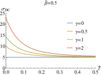
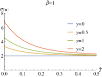
Figure 1: $\sigma_{DC}$ as the function of $\hat{T}$ for some specific $\gamma$ and $\hat{\beta}$.

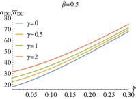
Figure 2: $\alpha_{DC},\bar{\alpha}_{DC}$ as the function of $\hat{T}$ for some specific $\gamma$ and $\hat{\beta}$.

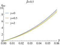
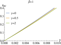
Figure 3: $\bar{\kappa}_{DC}$ as the function of $\hat{T}$ for some specific $\gamma$ and $\hat{\beta}$.

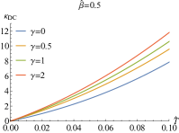
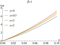
Figure 4: $\kappa_{DC}$ as the function of $\hat{T}$ for some specific $\gamma$ and $\hat{\beta}$.

Another quantities of interest are the Lorentz rations, which are the rations of thermal conductivity to electric conductivity

$$\bar{L}=\frac{\bar{\kappa}}{\sigma\hat{T}\mu_{\text{BI}}}=\frac{16\pi^{2}}{\hat{\beta}^{2}\mu_{\text{BI}}^{2}\sqrt{\gamma\mu^{2}+1}+\mu^{2}}\,,\$$ (31)

$$L=\frac{\kappa}{\sigma\hat{T}\mu_{\text{BI}}}=\frac{16\pi^{2}\hat{\beta}^{2}\mu_{\text{BI}}^{2}\sqrt{\gamma\mu^{2}+1}}{\left(\hat{\beta}^{2}\mu_{\text{BI}}^{2}\sqrt{\gamma\mu^{2}+1}+\mu^{2}\right){}^{2}}\,.$$ (32)

Obviously, $L$ is not a constant and so the Wiedemann-Franz law that $L$ is a constant for Fermi liquid Mahajan:2013cja is violated, which has been revealed in Donos:2014cya ; Kim:2014bza ; Kuang:2017rpx and indicates that our dual system involves strong interactions. Similarly with that in holographic Q-lattice model or linear axions model with standard Maxwell theory studied in Donos:2014cya , as $\hat{\beta}\rightarrow 0$, $\bar{L}$ and $\kappa$ approach the constants. It is interesting to notice that in this case, i.e., $\hat{\beta}\rightarrow 0$, $\bar{L}$ is independent of the BI parameter $\gamma$ but $\kappa$ depends on it, while $L$ vanishes and $\bar{\kappa}$ diverges in this limit which is similar to that observed in Donos:2014cya . In addition, the bound $\bar{L}\leq\frac{s^{2}}{Q}$ with $s$ being the entropy density of the black brane proposed in Donos:2014cya holds in our model.

IV Optical electric conductivity

In this section, we turn to study the AC electric conductivity by turning on the following consistent frequency dependent perturbations

$$\delta A_{x}=\int\frac{d\omega}{2\pi}e^{-i\omega t}a_{x}(u)\,,~{}~{}\delta g_{tx}=\int\frac{d\omega}{2\pi}e^{-i\omega t}\frac{h_{tx}(u)}{u^{2}}\,,~{}~{}\delta\phi_{x}=\int\frac{d\omega}{2\pi}e^{-i\omega t}\chi_{x}(u)\,.$$ (33)

Thus, the linearized equations of motion around the background (8) can be derived in momentum space as

$$a_{x}^{\prime}(u)\left(2\gamma u^{3}A_{t}^{\prime}(u){}^{2}+\frac{f^{\prime}(u)}{f(u)}\right)+\frac{\omega^{2}a_{x}(u)}{f(u)^{2}}+a_{x}^{\prime\prime}(u)+\frac{A_{t}^{\prime}(u)h_{\text{tx}}^{\prime}(u)}{f(u)}=0\,,\$$ (34)

$$4u^{2}\omega a_{x}(u)A_{t}^{\prime}(u)+\sqrt{1-\gamma u^{4}A_{t}^{\prime}(u){}^{2}}\left(\omega h_{\text{tx}}^{\prime}(u)-\alpha f(u)\chi_{x}^{\prime}(u)\right)=0\,,\$$ (35)

$$\left(\frac{f^{\prime}(u)}{f(u)}-\frac{2}{u}\right)\chi_{x}^{\prime}(u)-\frac{\alpha\omega h_{\text{tx}}(u)}{f(u)^{2}}+\frac{\omega^{2}\chi_{x}(u)}{f(u)^{2}}+\chi_{x}^{\prime\prime}(u)=0\,.$$ (36)

According to AdS/CFT dictionary, we can numerically solve the above equations and read off the AC conductivity by using the expression

$$\sigma(\omega)=\frac{\partial_{u}a_{x}}{i\omega a_{x}}\,.$$ (37)

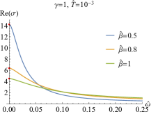
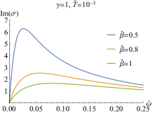
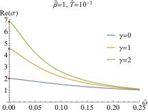
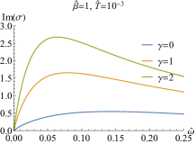
Figure 5: The electric conductivity $\sigma(\hat{\omega})$ for different $\hat{\beta}$ and $\gamma$.

We will explore the AC electric conductivity from non-linear BI electrodynamics with momentum dissipation. We shall fix the temperature $\hat{T}$ to study the effects of $\hat{\beta}$ and $\gamma$. FIG.5 exhibits the electric conductivity as the function of the frequency $\hat{\omega}$ for different $\hat{\beta}$ and $\gamma$. Similarly with the standard Maxwell theory, for the fixed $\gamma$, with the increase of $\hat{\beta}$, the Drude-like peak gradually reduces and a transition from coherent phase to incoherent phase happens. For the fixed $\hat{\beta}$, the peak seems to augment when $\gamma$ increases. But the quantitative analysis later indicates that although with the increase of $\gamma$ the peak augments, the degree of deviation from the Drude one becomes grave. Note that as a quick check on the consistency of our numerics, we denote the DC electric conductivity analytically calculated by (25) (red points) in FIG.5, which match very well with the numerical results.

Next we discuss the coherent and incoherent behavior of our present model by quantitatively exploring the low frequency behavior of the AC conductivity. It is well known that for the standard Maxwell theory, when the momentum dissipation is weak, i.e. $\hat{\beta}\ll 1$, the conductivity at low frequency can be described by the standard Drude formula,

$$\sigma(\hat{\omega})=\frac{K}{\Gamma-i\hat{\omega}}\,,$$ (38)

where $K$ is a constant and $\Gamma$ the momentum relaxation rate. It is the coherent transport. With the increase of $\hat{\beta}$, there is a crossover from coherent to incoherent phase, which can be depicted by the following modified Drude formula

$$\sigma(\hat{\omega})=\frac{K}{\Gamma-i\hat{\omega}}+\sigma_{Q}\,.$$ (39)

The above formula can be obtained in relativistic conformal hydrodynamics Hartnoll:2007ih and $\sigma_{Q}$ is the intrinsic conductivity of the hydrodynamic state, characterizing the incoherent contribution. In holographic framework, this formula has also been widely applied to study the coherent and incoherent behavior, for example, see Kim:2014bza ; Ling:2015exa ; Kuang:2017cgt .

Here, we shall study the low frequency conductivity behavior by using these two formulas and intend to give some quantitative discussions and insights into it.

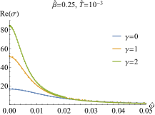
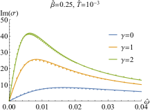
Figure 6: The electric conductivity $\sigma(\hat{\omega})$ for different $\gamma$ and the fixed $\hat{\beta}=0.25$. The dots are the numerical results while the solid lines are fitted by the standard Drude formula (38).

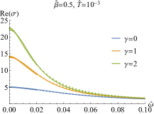
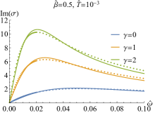
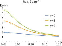
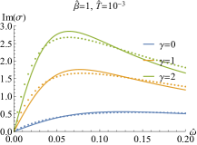
Figure 7: The electric conductivity $\sigma(\hat{\omega})$ for different $\gamma$ and $\hat{\beta}$ (the plots above is for $\hat{\beta}=0.5$ and the ones below for $\hat{\beta}=1$). The dots are the numerical results while the solid lines are fitted by the Modified Drude formula (39).

FIG.6 shows the electric conductivity $\sigma(\hat{\omega})$ for weak momentum dissipation ($\hat{\beta}=0.25$). It can fitted very well by the standard Drude formula (38) and we conclude that when the momentum dissipation is weak, the electric transport from BI-axions model is coherent for different BI coupling parameter $\gamma$. Quantitatively, the momentum relaxation rate $\Gamma$ decreases with the increase of $\gamma$ (see TABLE 1). When $\hat{\beta}=0.5$, we need resort to the modified Drude formula (39) to fit the numerical data. The results are shown in the above plots in FIG.7, which is fitted very well. It indicates a crossover from coherent to incoherent phase begins to appear around $\hat{\beta}\simeq 0.5$. Similarly with the weakly momentum dissipation case, the momentum relaxation rate $\Gamma$ also decreases with the increase of $\gamma$ in the crossover region (see TABLE 2). But we note that although the peak in $Re(\sigma)$ enhances, the $\sigma_{Q}$, the quantity characterizing the incoherent degree, increases with the increase of $\gamma$, which indicates that the BI coupling amplifies the incoherent behavior. With the further increase of $\hat{\beta}$, the incoherent behavior becomes stronger (see the plots below in FIG.7 and TABLE 3).

$\gamma$	$0$	$1$	$2$
$\Gamma$	$0.0165$	$0.00827$	$0.00630$

Table 1: The momentum relaxation rate $\Gamma$ fitted by the standard Drude formula (38) for different $\gamma$ with fixed $\hat{\beta}=0.25$.

$\gamma$	$0$	$1$	$2$
$\Gamma$	$0.0490$	$0.0264$	$0.0209$
$\sigma_{Q}$	$0.621$	$0.751$	$0.847$

Table 2: The momentum relaxation rate $\Gamma$ fitted by the modified Drude formula (39) for different $\gamma$ with fixed $\hat{\beta}=0.5$.

$\gamma$	$0$	$1$	$2$
$\Gamma$	$0.125$	$0.0770$	$0.0644$
$\sigma_{Q}$	$0.819$	$0.792$	$0.806$

Table 3: The momentum relaxation rate $\Gamma$ fitted by the modified Drude formula (39) for different $\gamma$ with fixed $\hat{\beta}=1$.

V Non-linear electric conductivity in probe limit

As is discussed in Baggioli:2016oju , the usual way to study non-linear conductivity is to show the non-linear current-voltage diagram, from which we may see the non-linear behavior of the electric conductivity. To get analytical control, we will work in the probe limit, i.e., we ignore the mixture with the metric perturbation and keep the non-linear self -couplings of the Maxwell field as done in the references Sonner:2012if ; Horowitz:2013mia .

We obtained in previous sections that $\sigma_{DC}$ is constant for fixed bulk parameters, that is to say, the DC conductivity is linear. Here we shall discuss the non-linear DC case via the steps in Baggioli:2016oju . Consider the gauge field as $A=A_{t}(u)dt+(E_{x}t+a_{x}(u))dx$, the Maxwell equations with the same form as (8) give us

$$\dot{\mathcal{L}_{BI}}A_{t}^{\prime}=-\rho,~{}~{}~{}\dot{\mathcal{L}_{BI}}f(u)a_{x}^{\prime}=-J_{x}$$ (40)

where $\dot{\mathcal{L}_{BI}}$ denotes the derivative to the field strength $I=-F^{2}/2$ and prime denotes the derivative to the radius $u$ . $\mathcal{L}_{BI}$ has been defined in (1) while the integration constants $\rho$ and $J_{x}$ are interpreted as charge density and charge current. Further requiring the field strength

$$I=u^{4}(A_{t}^{{}^{\prime}2}+\frac{E_{x}^{2}}{f(u)}-f(u)a_{x}^{{}^{\prime}2})$$ (41)

is regular at the horizon, we obtain the genera l current- voltage relation

$$J_{x}=\dot{\mathcal{L}_{BI}}\mid_{u_{h}}E_{x}.$$ (42)

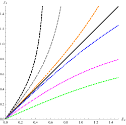
Figure 8: The current-voltage behavior for BI model. We set $\mu=u_{h}=1$, and the parameter $\gamma$ from top to down is $1,0.5,0.1,0,-0.1,-0.5,-0.8$.

The current- voltage behavior from (42) is shown in FIG. 8. $\gamma=0$ corresponds to the standard Maxwell theory, so that the current- voltage relation is linear and means $J_{x}=E_{x}$ as we expect. When $\gamma\neq 0$, the non-linear behavior is observed. For $\gamma>0$, the curve is above the linear case and $dJ_{x}/dE_{x}$ is stronger than $1$ as that happened in DBI modelBaggioli:2016oju , however, it is enhanced as the applied field $E_{x}$ increases which is different from that in DBI model. For $\gamma<0$, the non-linear $dJ_{x}/dE_{x}$ is always lower than $1$. As the applied field increases, it approaches to be vanished, but this will not happen because backreacion should be involved when $E_{x}$ is very large . The unstable case $dJ_{x}/dE_{x}<0$ shown in iDBI model is not observed in our model. We notice that when we continue to lower $\gamma$, the current become complex, this deserves further study.

VI Conclusions

In this paper, we introduced the Maxwell field with Born-Infeld correction into the Einstein-axions theory and constructed a new charged BI-AdS black hole. Then we analytically calculated various DC transport coefficients of the dual boundary theory. We found that the DC electric conductivity depends on the temperature of the boundary theory, which is a novel property comparing to that in RN-AdS black hole. At zero temperature, The DC electric conductivity are positive while the thermal conductivity vanishes. This means that the dual sector is an electrical metal but thermal insulator. With the increase of Born-Infeld parameter, the electric conductivity, electric-thermo conductivity and thermal conductivity at zero increases at finite fixed temperature.

We also studied the AC electric conductivity of the theory. When the momentum dissipation is weak, the low frequency AC conductivity behaves as the standard Drude formula and the electric transport is coherent for various correction parameter. When the momentum dissipation is stronger, the modified Drude formula is applied and a crossover from coherent to incoherent phase was observed. Also, we found that the Born-Infeld correction makes the incoherent behavior more explicit. We notice that here we only numerically compute the AC electric conductivity dual to its simply. It would be very interesting to further study the AC thermal and electric-thermo conductivity which are related with boundary data of both Maxwell perturbation and gravitational perturbationAmoretti:2014zha . We hope to show the results elsewhere soon.

Finally, we analyze the non-linear current-voltage behavior with BI correction in probe limit. The curve with $\gamma>0$ is above the linear case and $dJ_{x}/dE_{x}$ is always bigger than $1$. Different from that happened in DBI model Baggioli:2016oju , the slope is enhanced as $E_{x}$ increases. For $\gamma<0$, the non-linear $dJ_{x}/dE_{x}$ is always lower than $1$ and it tends to be zero as $E_{x}$ go to infinity in which case the backreaction should be considered. For more negative $\gamma$, the current become complex and further study is called for.

There are many interesting questions deserving further exploration. First of all, we can study the holographic anomalous transport from BI electrodynamics as Chu:2018ksb ; Chu:2018ntx . In Li:2017nxh ; Mokhtari:2017vyz , they study the thermal transport and quantum chaos in the EMDA theory with a small Weyl coupling term. In particular, in Li:2017nxh , they find that the Weyl coupling correct the thermal diffusion constant and butterfly velocity in different ways, hence resulting in a modified relation between the two at IR fixed points. It is interesting to further explore this relation in present of BI correction. We shall come back these topics in near future.

- (1) J. M. Maldacena, “The large N limit of superconformal field theories and supergravity,” Adv. Theor. Math. Phys. 2 (1998) 231 [Int. J. Theor. Phys. 38 (1999) 1113].
- (2) S. S. Gubser, I. R. Klebanov and A. M. Polyakov, “A semiclassical limit of the gauge string correspondence,” Nucl. Phys. B 636 (2002) 99.
- (3) E. Witten, “Anti-de Sitter space and holography, ” Adv. Theor. Math. Phys. 2 (1998) 253.
- (4) D. Vegh, “Holography without translational symmetry,” arXiv:1301.0537 [hep-th].
- (5) R. A. Davison, “Momentum relaxation in holographic massive gravity,” Phys. Rev. D 88, 086003 (2013) [arXiv:1306.5792 [hep-th]].
- (6) M. Blake and D. Tong, “Universal Resistivity from Holographic Massive Gravity,” Phys. Rev. D 88, no. 10, 106004 (2013) [arXiv:1308.4970 [hep-th]].
- (7) M. Blake, D. Tong and D. Vegh, “Holographic Lattices Give the Graviton an Effective Mass,” Phys. Rev. Lett. 112, no. 7, 071602 (2014) [arXiv:1310.3832 [hep-th]].
- (8) A. Amoretti, A. Braggio, N. Maggiore, N. Magnoli and D. Musso, “Analytic dc thermoelectric conductivities in holography with massive gravitons,” Phys. Rev. D 91, no. 2, 025002 (2015) [arXiv:1407.0306 [hep-th]].
- (9) Z. Zhou, J. P. Wu and Y. Ling, “DC and Hall conductivity in holographic massive Einstein-Maxwell-Dilaton gravity,” JHEP 1508, 067 (2015) [arXiv:1504.00535 [hep-th]].
- (10) M. Reza Mohammadi Mozaffar, A. Mollabashi and F. Omidi, “Non-local Probes in Holographic Theories with Momentum Relaxation,” JHEP 1610, 135 (2016) [arXiv:1608.08781 [hep-th]].
- (11) M. Baggioli and O. Pujolas, “Electron-Phonon Interactions, Metal-Insulator Transitions, and Holographic Massive Gravity,” Phys. Rev. Lett. 114, no. 25, 251602 (2015) [arXiv:1411.1003 [hep-th]].
- (12) L. Alberte, M. Baggioli, A. Khmelnitsky and O. Pujolas, “Solid Holography and Massive Gravity,” JHEP 1602, 114 (2016) [arXiv:1510.09089 [hep-th]].
- (13) M. Baggioli and O. Pujolas, “On holographic disorder-driven metal-insulator transitions,” JHEP 1701, 040 (2017) [arXiv:1601.07897 [hep-th]].
- (14) H. B. Zeng and J. P. Wu, “Holographic superconductors from the massive gravity,” Phys. Rev. D 90, no. 4, 046001 (2014) [arXiv:1404.5321 [hep-th]].
- (15) A. Amoretti, A. Braggio, N. Maggiore, N. Magnoli and D. Musso, “Thermo-electric transport in gauge/gravity models with momentum dissipation,” JHEP 1409, 160 (2014) [arXiv:1406.4134 [hep-th]];
- (16) A. Amoretti and D. Musso, “Magneto-transport from momentum dissipating holography,” JHEP 1509, 094 (2015) [arXiv:1502.02631 [hep-th]].
- (17) L. Q. Fang, X. M. Kuang and J. P. Wu, “The holographic fermions dual to massive gravity,” Sci. China Phys. Mech. Astron. 59, no. 10, 100411 (2016).
- (18) X. M. Kuang, E. Papantonopoulos, J. P. Wu and Z. Zhou, Phys. Rev. D 97, no. 6, 066006 (2018) [arXiv:1709.02976 [hep-th]].
- (19) G. T. Horowitz, J. E. Santos and D. Tong, “Optical Conductivity with Holographic Lattices,” JHEP 1207, 168 (2012) [arXiv:1204.0519 [hep-th]].
- (20) G. T. Horowitz, J. E. Santos and D. Tong, “Further Evidence for Lattice-Induced Scaling,” JHEP 1211, 102 (2012) [arXiv:1209.1098 [hep-th]].
- (21) Y. Ling, C. Niu, J. P. Wu and Z. Y. Xian, “Holographic Lattice in Einstein-Maxwell-Dilaton Gravity,” JHEP 1311, 006 (2013) [arXiv:1309.4580 [hep-th]].
- (22) A. Aperis, P. Kotetes, E. Papantonopoulos, G. Siopsis, P. Skamagoulis and G. Varelogiannis, “Holographic Charge Density Waves,” Phys. Lett. B 702, 181 (2011) [arXiv:1009.6179 [hep-th]].
- (23) A. Donos and J. P. Gauntlett, “Holographic charge density waves,” Phys. Rev. D 87, no. 12, 126008 (2013) [arXiv:1303.4398 [hep-th]].
- (24) Y. Ling, C. Niu, J. Wu, Z. Xian and H. b. Zhang, “Metal-insulator Transition by Holographic Charge Density Waves,” Phys. Rev. Lett. 113, 091602 (2014) [arXiv:1404.0777 [hep-th]].
- (25) S. Cremonini, L. Li and J. Ren, “Holographic Pair and Charge Density Waves,” Phys. Rev. D 95, no. 4, 041901 (2017) [arXiv:1612.04385 [hep-th]].
- (26) R. G. Cai, L. Li, Y. Q. Wang and J. Zaanen, “Intertwined Order and Holography: The Case of Parity Breaking Pair Density Waves,” Phys. Rev. Lett. 119, no. 18, 181601 (2017) [arXiv:1706.01470 [hep-th]].
- (27) A. Donos and J. P. Gauntlett, “Holographic Q-lattices,” JHEP 1404, 040 (2014) [arXiv:1311.3292 [hep-th]].
- (28) A. Donos and J. P. Gauntlett, “Novel metals and insulators from holography,” JHEP 1406, 007 (2014) [arXiv:1401.5077 [hep-th]].
- (29) Y. Ling, P. Liu, C. Niu and J. P. Wu, “Building a doped Mott system by holography,” Phys. Rev. D 92, no. 8, 086003 (2015) [arXiv:1507.02514 [hep-th]].
- (30) Y. Ling, P. Liu and J. P. Wu, “A novel insulator by holographic Q-lattices,” JHEP 1602, 075 (2016) [arXiv:1510.05456 [hep-th]].
- (31) A. Donos and S. A. Hartnoll, “Interaction-driven localization in holography,” Nature Phys. 9, 649 (2013) [arXiv:1212.2998 [hep-th]].
- (32) T. Andrade and B. Withers, “A simple holographic model of momentum relaxation,” JHEP 1405, 101 (2014) [arXiv:1311.5157 [hep-th]].
- (33) K. Y. Kim, K. K. Kim, Y. Seo and S. J. Sin, “Coherent/incoherent metal transition in a holographic model,” JHEP 1412, 170 (2014) [arXiv:1409.8346 [hep-th]].
- (34) L. Cheng, X. H. Ge and Z. Y. Sun, “Thermoelectric DC conductivities with momentum dissipation from higher derivative gravity,” JHEP 1504, 135 (2015) [arXiv:1411.5452 [hep-th]].
- (35) X. H. Ge, Y. Ling, C. Niu and S. J. Sin, “Thermoelectric conductivities, shear viscosity, and stability in an anisotropic linear axion model,” Phys. Rev. D 92, no. 10, 106005 (2015) [arXiv:1412.8346 [hep-th]].
- (36) T. Andrade, “A simple model of momentum relaxation in Lifshitz holography,” arXiv:1602.00556 [hep-th].
- (37) X. M. Kuang and J. P. Wu, “Thermal transport and quasi-normal modes in Gauss-Bonnet-axions theory,” Phys. Lett. B 770, 117 (2017) [arXiv:1702.01490 [hep-th]].
- (38) X. M. Kuang and E. Papantonopoulos, “Building a Holographic Superconductor with a Scalar Field Coupled Kinematically to Einstein Tensor,” JHEP 1608, 161 (2016) [arXiv:1607.04928 [hep-th]].
- (39) A. Cisterna, C. Erices, X. M. Kuang and M. Rinaldi, “Axionic black branes with conformal coupling,” arXiv:1803.07600 [hep-th].
- (40) M. R. Tanhayi and R. Vazirian, “Higher-curvature Corrections to Holographic Entanglement with Momentum Dissipation,” Eur. Phys. J. C 78, no. 2, 162 (2018) [arXiv:1610.08080 [hep-th]].
- (41) A. Cisterna, M. Hassaine, J. Oliva and M. Rinaldi, “Axionic black branes in the k-essence sector of the Horndeski model,” Phys. Rev. D 96, no. 12, 124033 (2017) [arXiv:1708.07194 [hep-th]].
- (42) A. Cisterna and J. Oliva, “Exact black strings and p-branes in general relativity,” Class. Quant. Grav. 35, no. 3, 035012 (2018) [arXiv:1708.02916 [hep-th]].
- (43) X. M. Kuang, E. Papantonopoulos, G. Siopsis and B. Wang, “Building a Holographic Superconductor with Higher-derivative Couplings,” Phys. Rev. D 88, 086008 (2013) [arXiv:1303.2575 [hep-th]].
- (44) J. Alsup, E. Papantonopoulos, G. Siopsis and K. Yeter, “Spontaneously Generated Inhomogeneous Phases via Holography,” Phys. Rev. D 88, no. 10, 105028 (2013) [arXiv:1305.2507 [hep-th]].
- (45) Y. Kats, L. Motl and M. Padi, “Higher-order corrections to mass-charge relation of extremal black holes,” JHEP 0712, 068 (2007) [hep-th/0606100].
- (46) D. Anninos and G. Pastras, “Thermodynamics of the Maxwell-Gauss-Bonnet anti-de Sitter black hole with higher derivative gauge corrections”, JHEP 07, 030 (2009).
- (47) N. Seiberg and E. Witten, “String theory and noncommutative geometry,” JHEP 9909, 032 (1999) [hep-th/9908142].
- (48) M. Hassaine and C. Martinez, “Higher-dimensional black holes with a conformally invariant Maxwell source,” Phys. Rev. D 75, 027502 (2007) [hep-th/0701058].
- (49) M. Born and L. Infeld, “Foundations of the new field theory,” Proc. Roy. Soc. Lond. A144 (1934) 425-451.
- (50) G. W. Gibbons, “Aspects of Born-Infeld theory and string / M theory,” Rev. Mex. Fis. 49S1, 19 (2003) [hep-th/0106059].
- (51) J. Jing and S. Chen, “Holographic superconductors in the Born-Infeld electrodynamics,” Phys. Lett. B 686, 68 (2010) [arXiv:1001.4227 [gr-qc]].
- (52) A. Sheykhi and F. Shaker, “Analytical study of holographic superconductor in Born CInfeld electrodynamics with backreaction,” Phys. Lett. B 754, 281 (2016) [arXiv:1601.04035 [hep-th]].
- (53) D. Ghorai and S. Gangopadhyay, “Higher dimensional holographic superconductors in Born CInfeld electrodynamics with back-reaction,” Eur. Phys. J. C 76, no. 3, 146 (2016) [arXiv:1511.02444 [hep-th]].
- (54) C. Lai, Q. Pan, J. Jing and Y. Wang, “On analytical study of holographic superconductors with Born CInfeld electrodynamics,” Phys. Lett. B 749, 437 (2015) [arXiv:1508.05926 [hep-th]].
- (55) P. Chaturvedi and G. Sengupta, “p-wave Holographic Superconductors from Born-Infeld Black Holes,” JHEP 1504, 001 (2015) [arXiv:1501.06998 [hep-th]].
- (56) N. Bai, Y. H. Gao, B. G. Qi and X. B. Xu, “Holographic insulator/superconductor phase transition in Born-Infeld electrodynamics,” arXiv:1212.2721 [hep-th].
- (57) S. Gangopadhyay and D. Roychowdhury, “Analytic study of Gauss-Bonnet holographic superconductors in Born-Infeld electrodynamics,” JHEP 1205 (2012) 156 [arXiv:1204.0673 [hep-th]].
- (58) S. Gangopadhyay and D. Roychowdhury, “Analytic study of properties of holographic superconductors in Born-Infeld electrodynamics,” JHEP 1205, 002 (2012) [arXiv:1201.6520 [hep-th]].
- (59) J. Jing, L. Wang, Q. Pan and S. Chen, “Holographic Superconductors in Gauss-Bonnet gravity with Born-Infeld electrodynamics,” Phys. Rev. D 83, 066010 (2011) [arXiv:1012.0644 [gr-qc]].
- (60) J. P. Wu, “Holographic fermionic spectrum from Born CInfeld AdS black hole,” Phys. Lett. B 758, 440 (2016) [arXiv:1705.06707 [hep-th]].
- (61) X. Guo, P. Wang and H. Yang, “Membrane Paradigm and Holographic DC Conductivity for Nonlinear Electrodynamics,” arXiv:1711.03298 [hep-th].
- (62) C. Charmousis, B. Gouteraux, B. S. Kim, E. Kiritsis and R. Meyer, “Effective Holographic Theories for low-temperature condensed matter systems,” JHEP 1011, 151 (2010) [arXiv:1005.4690 [hep-th]].
- (63) H. H. Soleng, “Charged black points in general relativity coupled to the logarithmic U(1) gauge theory,” Phys. Rev. D 52, 6178 (1995) [hep-th/9509033].
- (64) B. Mu, P. Wang and H. Yang, “Holographic DC Conductivity for a Power-law Maxwell Field,” arXiv:1711.06569 [hep-th].
- (65) S. Cremonini, A. Hoover and L. Li, “Backreacted DBI Magnetotransport with Momentum Dissipation,” JHEP 1710, 133 (2017) [arXiv:1707.01505 [hep-th]].
- (66) E. Kiritsis and L. Li, “Quantum Criticality and DBI Magneto-resistance,” J. Phys. A 50, no. 11, 115402 (2017) [arXiv:1608.02598 [cond-mat.str-el]].
- (67) I. M. Hayes, R. D. McDonald, N. P. Breznay, T. Helm, P. J. W. Moll, M. Wartenbe, A. Shekhter, J. G. Analytis, “Scaling between magnetic field and temperature in the high-temperature superconductor ,” Nature Physics 12, 916 (2016) [arXiv:1412.6484 [cond-mat.str-el]].
- (68) M. Baggioli and O. Pujolas, “On Effective Holographic Mott Insulators,” JHEP 1612 (2016) 107 [arXiv:1604.08915 [hep-th]].
- (69) T. K. Dey, “Born-Infeld black holes in the presence of a cosmological constant,” Phys. Lett. B 595, 484 (2004) [hep-th/0406169].
- (70) R. G. Cai, D. W. Pang and A. Wang, “Born-Infeld black holes in (A)dS spaces,” Phys. Rev. D 70, 124034 (2004) [hep-th/0410158].
- (71) R. G. Cai and Y. W. Sun, “Shear Viscosity from AdS Born-Infeld Black Holes,” JHEP 0809, 115 (2008) [arXiv:0807.2377 [hep-th]].
- (72) R. Banerjee and D. Roychowdhury, “Critical phenomena in Born-Infeld AdS black holes,” Phys. Rev. D 85, 044040 (2012) [arXiv:1111.0147 [gr-qc]].
- (73) Y. Liu and B. Wang, “Perturbations around the AdS Born-Infeld black holes,” Phys. Rev. D 85, 046011 (2012) [arXiv:1111.6729 [gr-qc]].
- (74) A. Donos and J. P. Gauntlett, “Thermoelectric DC conductivities from black hole horizons,” JHEP 1411, 081 (2014) [arXiv:1406.4742 [hep-th]].
- (75) M. Blake and A. Donos, Phys. Rev. Lett. 114, no. 2, 021601 (2015) [arXiv:1406.1659 [hep-th]].
- (76) R. Mahajan, M. Barkeshli and S. A. Hartnoll, “Non-Fermi liquids and the Wiedemann-Franz law,” Phys. Rev. B 88, 125107 (2013) [arXiv:1304.4249 [cond-mat.str-el]].
- (77) S. A. Hartnoll, P. K. Kovtun, M. Muller and S. Sachdev, “Theory of the Nernst effect near quantum phase transitions in condensed matter, and in dyonic black holes,” Phys. Rev. B 76, 144502 (2007) [arXiv:0706.3215 [cond-mat.str-el]].
- (78) J. Sonner and A. G. Green, “Hawking Radiation and Non-equilibrium Quantum Critical Current Noise,” Phys. Rev. Lett. 109, 091601 (2012) [arXiv:1203.4908 [cond-mat.str-el]].
- (79) G. T. Horowitz, N. Iqbal and J. E. Santos, “Simple holographic model of nonlinear conductivity,” Phys. Rev. D 88, no. 12, 126002 (2013) [arXiv:1309.5088 [hep-th]].
- (80) C. S. Chu and R. X. Miao, “Anomaly Induced Transport in Boundary Quantum Field Theories,” arXiv:1803.03068 [hep-th].
- (81) C. S. Chu and R. X. Miao, “Anomalous Transport in Holographic Boundary Conformal Field Theories,” arXiv:1804.01648 [hep-th].
- (82) W. J. Li, P. Liu and J. P. Wu, “Weyl corrections to diffusion and chaos in holography,” JHEP 1804, 115 (2018) [arXiv:1710.07896 [hep-th]].
- (83) A. Mokhtari, S. A. Hosseini Mansoori and K. Bitaghsir Fadafan, “Diffusivities bounds in the presence of Weyl corrections,” arXiv:1710.03738 [hep-th].