Supplementary Material — SmoothOut: Smoothing Out Sharp Minima to Improve Generalization in Deep Learning

Abstract

This supplementary material includes the proofs of Theorem 1 and Theorem 2, sensitivity analyses, and sharpness visualization.

Proof of Theorem LABEL:theorem1 and Theorem LABEL:theorem2

Proof of Theorem LABEL:theorem1:

Proof.

As $\mathcal{D}(\bm{w},a)$ is defined as a box centering at $\bm{w}$ with size $2a$, i.e.,

$$\mathcal{D}(\bm{w},a)=\left\{\bm{w}^{\prime}\in\mathbb{R}^{m}:|(\bm{w}^{\prime}-\bm{w})_{i}|\leq a,\forall i\in\{1...m\}\right\}\\ ,$$ (1)

then, under Uniform Perturbation,

$$\begin{split}\bar{C}(\bm{w})&=\textbf{E}\left\{\tilde{C}(\bm{w};\bm{\Theta})\right\}=\textbf{E}\left\{C(\bm{w}+\bm{\Theta})\right\}\\ &=\frac{1}{(2a)^{m}}\underset{\mathcal{D}(\bm{w},a)}{\idotsint}C(\bm{w}^{\prime})dw^{\prime}_{1}\dots dw^{\prime}_{m}\end{split}$$ (2)

$$\begin{split}&\frac{\partial\bar{C}(\bm{w})}{\partial w_{i}}=\frac{1}{(2a)^{m}}\cdot\\ &\underset{\mathcal{D}(\bm{w}_{\textbackslash i},a)}{\idotsint}\left(C(\bm{w}^{\prime})|_{w^{\prime}_{i}=w_{i}+a}-C(\bm{w}^{\prime})|_{w^{\prime}_{i}=w_{i}-a}\right)d\bm{w}^{\prime}_{\textbackslash i},\end{split}$$ (3)

where

$$\bm{w}_{\textbackslash i}\triangleq[w_{1},\cdots,w_{i-1},w_{i+1},\cdots,w_{m}]^{T}\in\mathbb{R}^{m-1}$$ (4)

and

$$d\bm{w}^{\prime}_{\textbackslash i}\triangleq dw^{\prime}_{1}\dots dw^{\prime}_{i-1}dw^{\prime}_{i+1}\dots dw^{\prime}_{m}\cdot$$ (5)

When $C(\bm{w})$ is symmetric about $\bm{w}_{f}$ in $\mathcal{D}(\bm{w}_{f},\tau){}$ such that, $\forall i$, a cut along $w_{i}=(\bm{w}_{f})_{i}+a$ and a cut along $w_{i}=(\bm{w}_{f})_{i}-a$ get the same function in the subspace $\bm{w}_{\textbackslash i}$, then $\nabla\bar{C}(\bm{w}_{f})=\bm{0}$; that is, the Flat Constraint satisfies with $\varphi=0$. ∎

The optimal $\varphi$ and $\tau$ are determined by the symmetry of the flat region. $\varphi$ may be relaxed to a larger value when the symmetry is broken; however, within a flat region, a larger $\varphi$ may only slightly increase $C(\bm{w}^{*})$.

Proof of Theorem LABEL:theorem2:

Proof.

Suppose $C^{(s)}_{\varepsilon^{\prime}}$ is the maximum value near the sharp minimum, i.e.,

$$C^{(s)}_{\varepsilon^{\prime}}=\underset{\mathcal{D}(\bm{w}_{s},\varepsilon^{\prime})}{\max}\left(C(\bm{w})\right),$$ (6)

as $C(\bm{w})$ is strictly monotonic in $\mathcal{D}(\bm{w}_{s},b)$, we have, $\forall\varepsilon^{\prime}<a<b$,

$$\underset{\mathcal{D}(\bm{w}_{s},a)\backslash\mathcal{D}(\bm{w}_{s},\varepsilon^{\prime})}{\min}\left(C(\bm{w})\right)>C^{(s)}_{\varepsilon^{\prime}},$$ (7)

where $\mathcal{D}(\bm{w}_{s},a)\backslash\mathcal{D}(\bm{w}_{s},\varepsilon^{\prime})$ is a Set Difference, notating a domain within $\mathcal{D}(\bm{w}_{s},a)$ but outside of $\mathcal{D}(\bm{w}_{s},\varepsilon^{\prime})$.

Then, follow the proof of Theorem LABEL:theorem1, we have

$$\begin{split}&\underset{\mathcal{D}(\bm{w}_{s},\varepsilon){}|_{\varepsilon<b}}{\min}\left(\bar{C}(\bm{w})\right)=\frac{1}{(2a)^{m}}\underset{\mathcal{D}(\bm{w}_{s},a)}{\idotsint}C(\bm{w}^{\prime})dw^{\prime}_{1}\dots dw^{\prime}_{m}\\ &\geq\frac{1}{(2a)^{m}}\cdot\left((2a)^{m}C^{(s)}_{\varepsilon^{\prime}}-(2\varepsilon^{\prime})^{m}\left(C^{(s)}_{\varepsilon^{\prime}}-C(\bm{w}_{s})\right)\right)\\ &=\left(1-\left(\frac{\varepsilon^{\prime}}{a}\right)^{m}\right)C^{(s)}_{\varepsilon^{\prime}}+\left(\frac{\varepsilon^{\prime}}{a}\right)^{m}\cdot C(\bm{w}_{s}).\end{split}$$ (8)

Because of

$$\lim_{m\to\infty}\left(\left(1-\left(\frac{\varepsilon^{\prime}}{a}\right)^{m}\right)C^{(s)}_{\varepsilon^{\prime}}+\left(\frac{\varepsilon^{\prime}}{a}\right)^{m}\cdot C(\bm{w}_{s})\right)=C^{(s)}_{\varepsilon^{\prime}},$$ (9)

in high dimensional models (like deep neural networks), we can find $\varepsilon\rightarrow\varepsilon^{\prime-}\rightarrow a^{-}$ (left limit) to satisfy

$$\underset{\mathcal{D}(\bm{w}_{s},\varepsilon){}}{\min}\left(\bar{C}(\bm{w})\right)>C^{(s)}_{\varepsilon}\triangleq\underset{\mathcal{D}(\bm{w}_{s},\varepsilon)}{\max}\left(C(\bm{w})\right).$$ (10)

In the flat region,

$$\begin{split}\underset{\mathcal{D}(\bm{w}_{f},\tau){}}{\min}\left(\bar{C}(\bm{w})\right)&=\frac{1}{(2a)^{m}}\underset{\mathcal{D}(\bm{w}_{f},a)}{\idotsint}C(\bm{w}^{\prime})dw^{\prime}_{1}\dots dw^{\prime}_{m}\\ &<\frac{1}{(2a)^{m}}\cdot\left((2a)^{m}\cdot\underset{\mathcal{D}(\bm{w}_{f},a)}{\max}\left(C(\bm{w})\right)\right)\\ &=\underset{\mathcal{D}(\bm{w}_{f},a)}{\max}\left(C(\bm{w})\right)\triangleq C^{(f)}_{a}\end{split}$$ (11)

Assuming $C(\bm{w}_{s})\approx C(\bm{w}_{f})$, as $a$ grows, $C^{(s)}_{\varepsilon}|_{\varepsilon\rightarrow a^{-}}$ increases fast in the sharp region while $C^{(f)}_{a}$ increases slowly in the flat region; therefore, $\exists a$ such that

$$C^{(s)}_{\varepsilon}>C^{(f)}_{a}.$$ (12)

According to Inequality (10)(11)(12),

$$\begin{split}\underset{\mathcal{D}(\bm{w}_{s},\varepsilon){}}{\min}\left(\bar{C}(\bm{w})\right)&>\underset{\mathcal{D}(\bm{w}_{s},\varepsilon)}{\max}\left(C(\bm{w})\right)\\ &>\underset{\mathcal{D}(\bm{w}_{f},a)}{\max}\left(C(\bm{w})\right)\\ &>\underset{\mathcal{D}(\bm{w}_{f},\tau){}}{\min}\left(\bar{C}(\bm{w})\right)\end{split}$$ (13)

which satisfies the Sharp Constraint. ∎

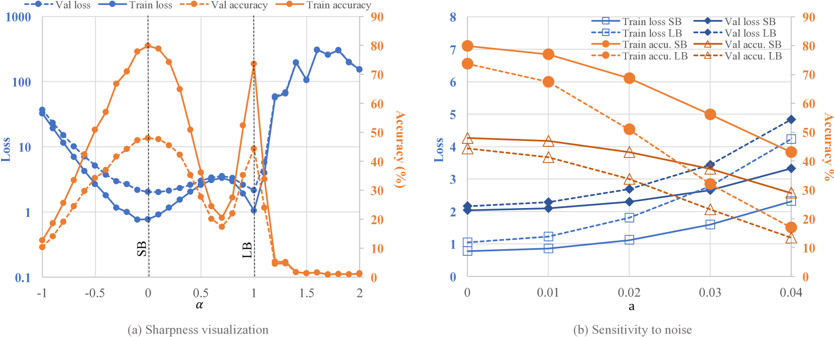
Figure 1: Notation:“SB”: Small Batch ($256$); “LB”: Large Batch ($5000$); “accu.”: accuracy. (a) loss and accuracy vs. $\alpha$, which controls $\bm{w}$ along the direction from SB minimum ($\bm{w}_{f}$) to LB minimum ($\bm{w}_{s}$); (b) loss and accuracy under influence of different strengths of noise. Dataset: CIFAR-100. Network: $C_{3}$. The optimizer is Adam with $0.001$ initial learning rate.

Figure 2: Loss and accuracy of ResNet-44 under influence of different strengths of noise on (a) CIFAR-10 and (b) CIFAR-100. The optimizer is SGD with momentum $0.9$. Notation:“SB”: Small Batch ($128$); “LB”: Large Batch ($2048$ for CIFAR-10 and $1024$ for CIFAR-100); “accu.”: accuracy.

Figure 3: Sharpness of baseline and SmoothOut in (a) “SB” training and (b) “LB” training of $C_{1}$.

Figure 4: Sharpness of baseline and SmoothOut in (a) “SB” training and (b) “LB” training of $F_{1}$.