A $\frac{5}{2}$-Approximation Algorithm for Coloring Rooted Subtrees of a Degree $3$ Tree

Abstract

A rooted tree $\vec{R}$ is a rooted subtree of a tree $T$ if the tree obtained by replacing the directed edges of $\vec{R}$ by undirected edges is a subtree of $T$. We study the problem of assigning minimum number of colors to a given set of rooted subtrees $\mathcal{R}$ of a given tree $T$ such that if any two rooted subtrees share a directed edge, then they are assigned different colors. The problem is NP hard even in the case when the degree of $T$ is restricted to $3$ [9]. We present a $\frac{5}{2}$-approximation algorithm for this problem. The motivation for studying this problem stems from the problem of assigning wavelengths to multicast traffic requests in all-optical WDM tree networks.

1 Introduction

1.1 Motivation

In Wavelength Division Multiplexing (WDM) [26] (p.208-211) multiple signals are transmitted simultaneously over a single optical fiber by using a different wavelength of light for each signal. The extremely high data transfer rate achievable by WDM, along with the low bit error rate have made it very attractive for backbone networks. Electronic switching becomes prohibitively expensive at this high data rate and hence switching is typically carried out in optical domain with the move between optical and electronic domains restricted to the source and the destination nodes. This scenario, in which a single lightpath is constructed between the source and the destination, is called transparent or all-optical networking. In absence of wavelength converters, which is usually the case due to their high cost, a lightpath must use the same wavelength on every fiber link on which it exists. This is called the wavelength continuity constraint. Also, if two lightpaths share a fiber link (in the same direction), then they must be assigned different wavelengths. In case of multicast traffic requests (single source-multiple destinations), in order to maintain transparent optics, network nodes capable of performing light splitting [25] and tap-and-continue operations [1] are employed. A single light tree is constructed from the source to the corresponding set of destinations to support a multicast request. The light is split and sent onto multiple fiber links on the nodes where bifurcation is required. On the intermediate nodes that are also in the destination set, a small amount of light is tapped and used to retrieve the data, while the rest of the light is allowed to travel through. The wavelength continuity constraint requires that the light tree use the same wavelength on every fiber link on which it exists. In case when the underlying fiber network is a tree, the routing of the light trees corresponding to the traffic requests is fixed and the given traffic requests can be treated as rooted subtrees of the underlying fiber tree. So the problem reduces to assigning a minimum number of wavelengths to these rooted subtrees such that any two rooted subtrees sharing a directed edge are assigned different wavelengths.

1.2 Notations and Definitions

$|S|$ denotes the cardinality of a finite set $S$. For real valued $x$, $[x]^{+}$ denotes $\max\{x,0\}$. $f(S)$ denotes the image of mapping $f:D\longrightarrow R$ restricted to set $S\subseteq D$.

Unless otherwise stated, all graphs are assumed to be simple. For graph $G$, $E_{G}$ and $V_{G}$ denote the edge set and the vertex set, respectively. An edge between vertices $u,v\in V_{G}$ is denoted by the set $\{u,v\}$. Similarly, for a directed graph $\vec{G}$, $E_{\vec{G}}$ and $V_{\vec{G}}$ denote the set of directed edges and vertices, respectively. For a pair of vertices $u,v\in V_{\vec{G}}$, a directed edge from $u$ to $v$ is denoted by the ordered pair $(u,v)$. $\bar{G}$ denotes the complement of graph $G$. $G[W]$ denotes the subgraph of graph $G$ induced by vertex set $W\subseteq V_{G}$.

The undirected multigraph obtained by replacing all the directed edges of directed graph $\vec{G}$ by undirected edges is referred to as the skeleton of $\vec{G}$. A directed graph $\vec{R}$ is a rooted tree if (i) its skeleton is a tree, (ii) there is a unique vertex $r\in V_{\vec{R}}$ with in-degree $0$, and (iii) every other vertex has in-degree $1$.A directed graph $\vec{R}$ is a rooted subtree of tree $T$ if $\vec{R}$ is a rooted tree and its skeleton is a subtree of $T$. In this case, we also refer to $T$ as the host tree of $\vec{R}$. Let $\mathcal{R}$ be a multiset of rooted subtrees of tree $T$. We denote the set of all the rooted subtrees in $\mathcal{R}$ that contain directed edge $(u,v)$ by $\mathcal{R}[(u,v)]$. If a rooted subtree $\vec{R}$ contains directed edge $(u,v)$, we say that it is present on the directed edge $(u,v)$. Moreover, the set $\mathcal{R}$ of rooted subtrees of the directed graph $\vec{G}$ collide on directed edge $(u,v)$, if for every rooted subtree $\vec{R}\in\mathcal{R}$, $(u,v)\in E_{\vec{R}}$. If the directed edge on which the collision occurs is not important for the subsequent discussion, we simply say that the set of rooted subtrees collide. With a slight abuse of notation, we denote the set of all rooted subtrees in $\mathcal{R}$ that contain either directed edge $(u,v)$ or $(v,u)$ by $\mathcal{R}[\{u,v\}]$. The load of a set $\mathcal{R}$ of rooted subtrees on a tree $T$ is defined to be the maximum number of rooted subtrees in that set that share a directed edge and is denoted by $l_{\mathcal{R}}$.

Let $\mathbb{N}$ denote the set of natural numbers. A valid coloring of a given set of rooted subtrees $\mathcal{R}$ of a tree $T$ is a map $\psi:\mathcal{R}\longrightarrow\mathbb{N}$ such that for any pair of rooted subtrees $\vec{R}_{i},\vec{R}_{j}\in\mathcal{R}$ that collide, $\psi(\vec{R}_{i})\neq\psi(\vec{R}_{j})$. We denote the set of all valid colorings by $\Psi_{\mathcal{R}}$. We can create a conflict graph for a given set of rooted subtrees $\mathcal{R}$ of a tree $T$ where the vertices represent the rooted subtrees and there is an edge between two vertices if the corresponding rooted subtrees collide. We denote this conflict graph by $G_{\mathcal{R}}$. Note that coloring rooted subtrees $\mathcal{R}$ is equivalent to coloring the vertices of $G_{\mathcal{R}}$.

1.3 Problem Statement

The coloring problem that we are interested in is stated as Problem 1.1 below.

Problem 1.1

Given a set of rooted subtrees $\mathcal{R}$ of a tree $T$ with degree at most $3$, find a coloring $\psi\in\Psi_{\mathcal{R}}$ that minimizes the number of colors used.

Note that assigning wavelengths to a set of multicast traffic requests in an all-optical WDM network where the underlying fiber topology is a tree $T$ is exactly equivalent to determining the coloring for the corresponding set of rooted subtrees $\mathcal{R}$.

1.4 Related Work

The work that is most closely related to the problem of coloring a given set of rooted subtrees of a tree, consists of the following:

• Coloring a given set of undirected paths on a tree.

• Coloring a given set of directed paths on a tree.

• Coloring and characterization of a given set of subtrees of a tree.

Our contribution can be seen as the next logical step in this series of works.

In [13], Golumbic et al. proved that determining a minimum coloring for a given set of undirected paths on a tree is NP hard in general. They showed that undirected path coloring in stars is equivalent to edge coloring in multigraphs. Since edge coloring is NP hard [18], undirected path coloring in stars is also NP hard. In fact, as observed in [10], this equivalence result has several important implications:

• Undirected path coloring is solvable in polynomial time in bounded degree trees.

• Undirected path coloring is NP hard for trees of arbitrary degrees (even with diameter 2).

• Any approximation algorithm for edge coloring in multigraphs can be modified into an approximation algorithm for undirected path coloring in trees and vice versa with the same approximation ratio.

• Approximating undirected path coloring in trees of arbitrary degree with an approximation ratio $\frac{4}{3}-\epsilon$ for any $\epsilon>0$ is NP hard.

In [30], Tarjan introduced a $\frac{3}{2}$-approximation algorithm for coloring a given set of undirected paths in a tree. Later, this ratio was rediscovered by Raghavan and Upfal [29] in the context of optical networks. Mihail et al. [27] presented a coloring scheme with an asymptotic approximation ratio of $\frac{9}{8}$. Nishizeki et al. [28] presented an algorithm for edge coloring multigraphs with an asymptotic approximation ratio of $1.1$ and an absolute approximation ratio of $\frac{4}{3}$. This improves the asymptotic and the absolute approximation ratio of undirected path coloring in trees to $1.1$ and $\frac{4}{3}$ respectively.

In [8], Erlebach et al. proved that coloring a given set of directed paths in trees is NP hard. The hardness result holds even when we restrict instances to arbitrary trees and sets of directed paths of load $3$ or to trees with arbitrary degree and depth $3$ [23]. For this problem, Mihail et al. [27] gave a $\frac{15}{8}$-approximation algorithm. This ratio was improved to $\frac{7}{4}$ in [21] and [24], and finally to $\frac{5}{3}$ in [22]. All these are greedy, deterministic algorithms and use the load of the given set of directed paths as the lower bound on the number of colors required. In [22], Kaklamanis et al. also proved that no greedy, deterministic algorithm can achieve a better approximation ratio than $\frac{5}{3}$.

Unlike its undirected counterpart, Erlebach et al. [9] proved by a reduction from circular arc coloring that the problem of coloring directed paths is NP hard even in binary trees. This result also implies that the problem that we are interested in is also NP hard. In [24], Kumar et al. gave a problem instance where the given set of directed paths on a binary tree of depth $3$ having load $l$ requires at least $\frac{5}{4}l$ colors. Caragiannis et al. [4] and Jansen [20] gave algorithms for the directed path coloring in binary trees having approximation ratio $\frac{5}{3}$ (same as for general trees). In [2], Auletta et al. presented a randomized greedy algorithm for coloring directed paths of maximum load $l$ in binary trees of depth $O(l^{\frac{1}{3}-\epsilon})$ that uses at most $\frac{7}{5}l+o(l)$ colors. They also proved that with high probability, randomized greedy algorithms cannot achieve an approximation ratio better than $\frac{3}{2}$ when applied for binary trees of depth $\Omega(l)$, and $1.293-o(1)$ when applied for binary trees of constant depth. Moreover, they proved an upper bound of $\frac{7}{5}l+o(l)$ for all binary trees. In [10], Erlebach et al. proved that approximating directed path coloring in binary trees with an approximation ratio $\frac{4}{3}-\epsilon$ for any $\epsilon>0$ is NP hard.

In [19] Jamison et al. proved that the conflict graphs of subtrees in a binary tree are chordal [11], and therefore easily colorable [12]. In [14] Golumbic et al. proved that the conflict graphs (obtained as described above) of undirected paths on degree $4$ trees are weakly chordal [16], therefore coloring them is easy [17]. Later, in [15], they extended the result to the conflict graph of subtrees on degree $4$ trees.

For an extensive compilation of complexity results on both directed and undirected paths in trees from the perspective of optical networks, the reader is referred to [23] and [10]. And for a survey of algorithmic results, the reader is referred to [5], [6] and [7].

Ours is the first work to study the problem of coloring rooted subtrees of a tree. As stated previously, this can be seen as the directed counterpart of the problem of coloring subtrees of a tree.

2 Algorithm

In this section, we present a greedy coloring scheme for Problem 1.1. The algorithm is presented as Algorithm 1 (GREEDY-COL). We denote the coloring generated by this algorithm as $\psi^{\mathrm{GDY}}$. The algorithm proceeds in rounds. In each round we select and process a host tree edge which has not been selected in any of the previous rounds. Processing a host tree edge means coloring all the uncolored rooted subtrees present on that edge.

Algorithm 1 GREEDY-COL

0:  Set of rooted subtrees $\mathcal{R}$ on host tree $T$ with degree at most $3$.

0:  A coloring $\psi^{\mathrm{GDY}}\in\Psi_{\mathcal{R}}$.

1:  Perform BFS on host tree $T$ starting with arbitrary vertex as the root and enumerate tree edges in the order of their discovery. Let $\{e_{1},\dots,e_{|E_{T}|}\}$ be the ordered set of edges $E_{T}$.

2:  $\mathcal{P}_{0}\leftarrow\emptyset$

3:  for $i=1$ to $|E_{T}|$ do

4:     $\mathcal{Q}_{i}\leftarrow\mathcal{R}[e_{i}]\setminus\mathcal{P}_{i-1}$

5:     if edge $e_{i}=\{u,v\}$ is of type $4$ as defined in Lemma 3.3 then

6:        Let $\psi_{1},\psi_{2}\in\Psi_{\mathcal{Q}_{i}\cup\mathcal{P}_{i-1}}$

7:        $\psi_{1}(\vec{R}),\psi_{2}(\vec{R})\leftarrow\psi^{\mathrm{GDY}}(\vec{R})$ for every $\vec{R}_{j}\in\mathcal{P}_{i-1}$ (uncolored otherwise).

8:        PROCESS-EDGE-1$(T,\{u,v\},\mathcal{P}_{i-1},\mathcal{Q}_{i},\psi_{1})$

9:        PROCESS-EDGE-2$(T,\{\{u,v\},\{u,w\},\{u,x\}\},\mathcal{P}_{i-1},\mathcal{Q}_{i},\psi_{2})$

10:        if $|\psi_{1}(\mathcal{P}_{i-1}\cup\mathcal{Q}_{i})|\leq|\psi_{2}(\mathcal{P}_{i-1}\cup\mathcal{Q}_{i})|$ then

11:           $\psi^{\mathrm{GDY}}(\vec{R})\leftarrow\psi_{1}(\vec{R})$ for every $\vec{R}\in\mathcal{Q}_{i}$

12:        else

13:           $\psi^{\mathrm{GDY}}(\vec{R})\leftarrow\psi_{2}(\vec{R})$ for every $\vec{R}\in\mathcal{Q}_{i}$

14:        end if

15:     else

16:        while $\exists$ some uncolored $\vec{R}\in\mathcal{Q}_{i}$ do

17:           $\psi^{\mathrm{GDY}}\!(\vec{R})\leftarrow\min\{l\in\mathbb{N}:\nexists\,\vec{S}\!\in\!\mathcal{P}_{i-1}\!\cup\!\mathcal{Q}_{i}\textrm{ s.t. }\vec{R},\vec{S}\textrm{ collide and }\psi^{\mathrm{GDY}}\!(\vec{S})\!=\!l\}$

18:        end while

19:     end if

20:     $\mathcal{P}_{i}\leftarrow\mathcal{P}_{i-1}\cup\mathcal{Q}_{i}$

21:  end for

2.1 Edge Order

We traverse the edges of the host tree in a breadth-first manner, i.e., starting with an arbitrary vertex as root, we perform a Breadth First Search (BFS) on the host tree $T$ and rank its edges in the order of their discovery, and then process the edges in this order. Let us assume that the set of edges $E_{H}$ in the order of enumeration is $\{e_{1},\dots,e_{|E_{H}|}\}$. In the $i$-th round of GREEDY-COL, edge $e_{i}$ is processed. GREEDY-COL involves exactly $|E_{T}|$ rounds of coloring.

2.2 Coloring Strategy

Let the set of rooted subtrees that are colored in the first $i$ rounds in GREEDY-COL be $\mathcal{P}_{i}$. We define $\mathcal{P}_{0}$ to be empty. The set of rooted subtrees present on edge $e_{i}$ but not in the set $\mathcal{P}_{i}$ is denoted by $\mathcal{Q}_{i}$, i.e., $\mathcal{Q}_{i}=\mathcal{R}[e_{i}]\setminus\mathcal{P}_{i}$. Note that $\mathcal{Q}_{i}$ is the set of rooted subtrees that are colored in the $i$-th round of GREEDY-COL.

The basic idea is to be greedy in each round of coloring and try to use as few new colors as possible while processing the edge.The actual coloring scheme followed in the $i$-th round of GREEDY-COL depends on the type of edge $e_{i}$ being processed. According to Lemma 3.3 below, tree edge $e_{i}$ encountered during the $i$-th round of GREEDY-COL can be classified into one of the four types (defined in the lemma) based on the status (whether already processed or not) of its adjacent tree edges. If edge $e_{i}$ is of type $1$, $2$, or $3$ as defined in Lemma 3.3, then uncolored rooted subtrees are randomly selected from the set $\mathcal{Q}_{i}$ one at a time and are colored. In more detail, suppose rooted subtree $\vec{R}$ has been selected from the set $\mathcal{Q}_{i}$ for coloring. If there is a color that has already been assigned to some rooted subtree(s) and can also be assigned to $\vec{R}$, then that color is assigned to $\vec{R}$, otherwise a new color (not assigned to any other rooted subtree previously) is assigned to $\vec{R}$.On the other hand, if edge $e_{i}$ is of type $4$ as defined in Lemma 3.3, then we assign colors to the rooted subtrees in the set $\mathcal{Q}_{i}$ according to the better of the two different coloring schemes presented as Subroutine 2 (PROCESS-EDGE-1) and Subroutine 3 (PROCESS-EDGE-2).

Subroutine 2 PROCESS-EDGE-1

0:  $\{T,\{u,v\}\in E_{T},\mathcal{P},\mathcal{Q},\psi\}$ s.t. degree of tree $T$ is at most $3$, $\mathcal{P}$ is set of rooted subtrees of $T$ that have already been colored according to $\psi:\mathcal{P}\longrightarrow\mathbb{N}$ and $\mathcal{Q}$ is set of all uncolored rooted subtrees of $T$ that are present on host tree edge $\{u,v\}$.

0:  Complete the given mapping $\psi$ to $\psi:\mathcal{P}\cup\mathcal{Q}\longrightarrow\mathbb{N}$ s.t. $\psi\in\Psi_{\mathcal{P}\cup\mathcal{Q}}$.

1:  $B_{1}\leftarrow G_{\mathcal{P}[\{u,v\}]\cup\mathcal{Q}}$

2:  for all pairs $\vec{R},\vec{S}\in\mathcal{P}[\{u,v\}]\cup\mathcal{Q}$ s.t. $\vec{R},\vec{S}$ do not collide do

3:     if any one of the following is true:

1. $\vec{R},\vec{S}\in\mathcal{P}$ and $\psi(\vec{R})\neq\psi(\vec{S})$.

2. $\vec{R}\in\mathcal{Q},\vec{S}\in\mathcal{P}$ and $\exists\,\vec{U}\in\mathcal{P}$ such that $\psi(\vec{S})=\psi(\vec{U})$ and $\vec{R},\vec{U}$ collide.

 then

4:        $E_{B_{1}}\leftarrow E_{B_{1}}\cup\;\{\{\vec{R},\vec{S}\}\}$

5:     end if

6:  end for

7:  Determine a maximum matching $M_{\bar{B}_{1}}\subseteq E_{\bar{B}_{1}}$. {$\bar{B}_{1}$ is bipartite.}

8:  for all matched edges $\{\vec{R},\vec{S}\}\in M_{\bar{B}_{1}}$ s.t. $\vec{R}\in\mathcal{Q}$ and $\vec{S}\in\mathcal{P}$ do

9:     $\psi(\vec{R})\leftarrow\psi(\vec{S})$

10:  end for

11:  while $\exists$ some uncolored $\vec{R}\in\mathcal{Q}$ do

12:     if $\exists$ matched edge $\{\vec{R},\vec{S}\}\in M_{\bar{B}_{1}}$ then

13:        $\psi(\vec{R}),\!\psi(\vec{S})\!\!\leftarrow\!\!\min\{m\!\in\!\mathbb{N}\!:\!\nexists\,\vec{U}\!\in\!\mathcal{P}\!\cup\!\mathcal{Q}\textrm{ s.t. }\vec{R},\!\vec{U}\textrm{ or }\vec{S},\!\vec{U}\textrm{ collide and }\psi(\vec{U})\!=\!m\}$

14:     else

15:        $\psi(\vec{R})\leftarrow\min\{m\in\mathbb{N}:\nexists\,\vec{U}\in\mathcal{P}\cup\mathcal{Q}\textrm{ s.t. }\vec{R},\vec{U}\textrm{ collide and }\psi(\vec{U})=m\}$

16:     end if

17:  end while

As we shall see in Lemma 3.3, edge $e_{i}=\{u,v\}$ being a type $4$ edge means that none of the tree edges adjacent to vertex $v$ have yet been processed and there are two edges adjacent to vertex $u$ (besides edge $e_{i}=\{u,v\}$), namely $\{u,w\}$ and $\{u,x\}$, of which edge $\{u,w\}$ has already been processed and edge $\{u,x\}$ has not yet been processed. The two coloring schemes employed while processing a type $4$ edge $e_{i}=\{u,v\}$ differ in the way they go about reusing the colors. In PROCESS-EDGE-1 we prefer to reuse colors from the set $\psi^{\mathrm{GDY}}(\mathcal{P}_{i-1}[\{u,v\}])$ (set of colors assigned to the rooted subtree(s) present on host tree edge $e_{i}=\{u,v\}$ that were colored in the first $i-1$ rounds), whereas in PROCESS-EDGE-2 we prefer to reuse colors from the set $\psi^{\mathrm{GDY}}(\mathcal{P}_{i-1}[\{u,x\}]\setminus\mathcal{P}_{i-1}[\{u,v\}])$ (set of colors assigned to the rooted subtree(s) present on host tree edge $\{u,x\}$, but not on tree edge $e_{i}=\{u,v\}$, that were colored in the first $i-1$ rounds). Note that the two sets of colors are not necessarily mutually exclusive. The two schemes also differ in the order in which uncolored rooted subtrees in the set $\mathcal{Q}_{i}$ are selected for coloring. More specifically, in PROCESS-EDGE-2, first colors are assigned to all the rooted subtrees in the set $\mathcal{Q}_{i}[\{u,x\}]$ and then to the rest of the uncolored rooted subtrees.

Subroutine 3 PROCESS-EDGE-2

0:  $\{T,\{\{u,v\},\{u,w\},\{u,x\}\}\subseteq E_{T},\mathcal{P},\mathcal{Q},\psi\}$ s.t. degree of tree $T$ is $3$, $\mathcal{P}$ is set of rooted subtrees of $T$ that have already been colored according to $\psi:\mathcal{P}\longrightarrow\mathbb{N}$ and $\mathcal{Q}$ is set of all uncolored rooted subtrees of $T$ that are present on host tree edge $\{v,u\}$.

0:  Complete the given mapping $\psi$ to $\psi:\mathcal{P}\cup\mathcal{Q}\longrightarrow\mathbb{N}$ s.t. $\psi\in\Psi_{\mathcal{P}\cup\mathcal{Q}}$.

1:  $B_{2}\leftarrow G_{\left(\mathcal{P}[\{u,x\}]\setminus\mathcal{P}[\{u,v\}]\right)\cup\mathcal{Q}[\{u,x\}]}$

2:  for all pairs $\vec{R},\vec{S}\!\in\!\left(\mathcal{P}[\{u,x\}]\!\setminus\!\mathcal{P}[\{u,v\}]\right)\cup\mathcal{Q}[\{u,x\}]$ s.t. $\vec{R},\vec{S}$ do not collide do

3:     if any one of the following is true:

1. $\vec{R},\vec{S}\in\mathcal{P}$ and $\psi(\vec{R})\neq\psi(\vec{S})$.

2. $\vec{R}\in\mathcal{Q},\vec{S}\in\mathcal{P}$ and $\exists\,\vec{U}\in\mathcal{P}$ s.t. $\psi(\vec{S})=\psi(\vec{U})$ and $\vec{R},\vec{U}$ collide.

 then

4:        $E_{B_{2}}\leftarrow E_{B_{2}}\cup\;\{\{\vec{R},\vec{S}\}\}$

5:     end if

6:  end for

7:  Determine a maximum matching $M_{\bar{B}_{2}}\subseteq E_{\bar{B}_{2}}$. {$\bar{B}_{2}$ is bipartite.}

8:  for all matched edges $\{\vec{R},\vec{S}\}\in M_{\bar{B}_{2}}$ s.t. $\vec{R}\in\mathcal{Q}$ and $\vec{S}\in\mathcal{P}$ do

9:     $\psi(\vec{R})\leftarrow\psi(\vec{S})$

10:  end for

11:  while $\exists$ some uncolored $\vec{R}\in\mathcal{Q}[\{u,x\}]$ do

12:     if $\exists$ matched edge $\{\vec{R},\vec{S}\}\in M_{\bar{B}_{2}}$ then

13:        $\psi(\vec{R}),\!\psi(\vec{S})\!\!\leftarrow\!\!\min\{m\!\in\!\mathbb{N}\!:\!\nexists\,\vec{U}\!\in\!\mathcal{P}\!\cup\!\mathcal{Q}\textrm{ s.t. }\vec{R},\!\vec{U}\textrm{ or }\vec{S},\!\vec{U}\textrm{ collide and }\psi(\vec{U})\!=\!m\}$

14:     else

15:        $\psi(\vec{R})\leftarrow\min\{m\in\mathbb{N}:\nexists\,\vec{U}\in\mathcal{P}\cup\mathcal{Q}\textrm{ s.t. }\vec{R},\vec{U}\textrm{ collide and }\psi(\vec{U})=m\}$

16:     end if

17:  end while

18:  while $\exists$ some uncolored $\vec{R}\in\mathcal{Q}$ do

19:     $\psi(\vec{R})\leftarrow\min\{m\in\mathbb{N}:\nexists\,\vec{U}\in\mathcal{P}\cup\mathcal{Q}\textrm{ s.t. }\vec{R},\vec{U}\textrm{ collide and }\psi(\vec{U})=m\}$

20:  end while

In PROCESS-EDGE-1 (line 7), we determine the maximum number of mutually exclusive pairs of rooted subtrees such that in each matched pair (say $\vec{R},\vec{S}$) at least one of the rooted subtrees (say $\vec{R}$) is an uncolored rooted subtree from the set $\mathcal{Q}_{i}$ (i.e., $\vec{R}\in\mathcal{Q}_{i}$) and the second rooted subtree ($\vec{S}$ in this case) may either be (i) another uncolored rooted subtree from the set $\mathcal{Q}_{i}$ (i.e., $\vec{S}\in\mathcal{Q}_{i}$) or (ii) a rooted subtree from the set $\mathcal{P}_{i-1}[e_{i}]$ such that the uncolored rooted subtree in the pair can be safely assigned its color (i.e., $\vec{S}\in\mathcal{P}_{i-1}$ such that $\vec{R}$ does not collide with any rooted subtree that has already been assigned the same color as $\vec{S}$). If the pair is of type (ii), then the uncolored rooted subtree is assigned the same color as the other rooted subtree (line 9). If the pair is of type (i), then both the rooted subtrees of the pair are assigned the same color (line 13). In this case, preference is given to the colors that have already been assigned to some rooted subtree(s). If there is no such suitable color, a new color is used.

In PROCESS-EDGE-2 (line 7), we determine the maximum number of mutually exclusive pairs of rooted subtrees such that in each matched pair (say $\vec{R},\vec{S}$) at least one of the rooted subtrees (say $\vec{R}$) is an uncolored rooted subtree from the set $\mathcal{Q}_{i}$ and is present on tree edge $\{u,x\}$ (i.e., $\vec{R}\in\mathcal{Q}_{i}[\{u,x\}]$) and the second rooted subtree ($\vec{S}$ in this case) may either be (i) another uncolored rooted subtree from the set $\mathcal{Q}_{i}$ present on edge $\{u,x\}$ (i.e., $\vec{S}\in\mathcal{Q}_{i}[\{u,x\}]$) or (ii) a rooted subtree from the set $\mathcal{P}_{i-1}[\{u,x\}]\setminus\mathcal{P}_{i-1}[\{u,v\}]$ such that the uncolored rooted subtree in the pair can be safely assigned its color (i.e., $\vec{S}\in\mathcal{P}_{i-1}[\{u,x\}]\setminus\mathcal{P}_{i-1}[\{u,v\}]$ such that $\vec{R}$ does not collide with any rooted subtree that has already been assigned the same color as $\vec{S}$). If the pair is of type (ii), then the uncolored rooted subtree is assigned the same color as the other rooted subtree (line 9). If the pair is of type (i), then both the rooted subtrees of the pair are assigned the same color (line 13). Again preference is given to the colors that have already been assigned to some rooted subtree(s). If there is no such suitable color, a new color is used. After this all the remaining uncolored rooted subtrees (all the rooted subtree in the set $\mathcal{Q}_{i}\setminus\mathcal{Q}_{i}[\{u,x\}]$ and possibly some rooted subtrees still uncolored in the set $\mathcal{Q}_{i}[\{u,x\}]$) are assigned colors one at a time (lines 15, 19). Again preference is given to the colors that have already been assigned to some rooted subtree(s).

3 Analysis

In this section, we shall prove that GREEDY-COL is a $\frac{5}{2}$-approximation algorithm for Problem 1.1.

3.1 Some Local Properties

We start off by stating a couple of straightforward but useful results about the local structure of the problem at hand. Since the lemmas are very simple, rather than complete proofs, we shall only give the intuition behind these.

Lemma 3.1

The complement of the conflict graph of any subset of rooted subtrees present on a single host tree edge is bipartite.

Lemma 3.2

If the load of the set $\mathcal{R}$ of rooted subtrees on the tree $T$ is $l_{\mathcal{R}}$ then there exists a set $\mathcal{S}\supseteq\mathcal{R}$ of rooted subtrees on the tree $T$ such that the following hold:

• The chromatic numbers of the conflict graphs $G_{\mathcal{S}}$ and $G_{\mathcal{R}}$ are the same.

• For every edge $\{u,v\}\in E_{T}$, $|\mathcal{S}[(u,v)]|=|\mathcal{S}[(v,u)]|=l_{\mathcal{S}}=l_{\mathcal{R}}$.

Moreover, $\mathcal{S}$ can be constructed in polynomial time.

Lemma 3.1 relies on two simple facts: (i) for any host tree edge $\{u,v\}\in E_{T}$, $\mathcal{R}[(u,v)]$ and $\mathcal{R}[(v,u)]$ partition $\mathcal{R}[\{u,v\}]$, and (ii) all rooted subtrees within each partition collide with every other rooted subtree in that partition. The construction of $\mathcal{S}$ in Lemma 3.2 can be achieved by going over every edge $\{u,v\}\in E_{T}$ and adding required number rooted subtrees containing only the vertices $u$ and $v$ and one directed edge (either $(u,v)$ or $(v,u)$ such that $|\mathcal{S}[(u,v)]|$ and $|\mathcal{S}[(v,u)]|$ become equal to $l_{\mathcal{R}}$. Lemma 3.2 allows us to study only those instances of the Problem 1.1 where the given set of rooted subtrees $\mathcal{R}$ is such that the number of rooted subtrees present on all directed edges is the same. Going forward we shall assume that for every edge $\{u,v\}\in E_{T}$, $|\mathcal{R}[(u,v)]|=|\mathcal{R}[(v,u)]|=l_{\mathcal{R}}$. Consequently, $|\mathcal{R}[\{u,v\}]|=2l_{\mathcal{R}}$.

3.2 Roadmap

First we give a roadmap that we shall follow for proving the approximation ratio of $\frac{5}{2}$ for GREEDY-COL.

• First, in Lemmas 3.3 and 3.4, we characterize the types of host tree edges that are encountered during any round of coloring in GREEDY-COL.

• Next, in Lemma 3.5, we prove that if the edge to be processed in $i$-th round of coloring is of type $1$, $2$ or $3$ as defined in Lemma 3.3, then either no new colors are required in the $i$-th round or the total number of colors in use at the end of the $i$-th round is less than or equal to $2l_{\mathcal{R}}$.

• If the edge to be processed in $i$-th round of coloring is of type $4$ as defined in Lemma 3.3, we first show in Lemma 3.6, that either no new color is required in the $i$-th round or the set of colors in use after $i$-th round of coloring is the same as the set of colors used for the rooted subtrees that are assigned colors in the $i$-th round ($\mathcal{Q}_{i}$) and all the rooted subtrees that are present on host tree edge $\{u,w\}$ which is adjacent to the edge being processed in the $i$-th round and has already been processed, i.e., $\psi^{\mathrm{GDY}}(\mathcal{Q}_{i}\cup\mathcal{P}_{i-1}[\{u,w\}])=\psi^{\mathrm{GDY}}(\mathcal{P}_{i})$. Next, we present bounds on the number of colors in the set $\mathcal{Q}_{i}\cup\mathcal{P}_{i-1}[\{u,w\}]$ when subroutines PROCESS-EDGE-1 (Lemma 3.7) or PROCESS-EDGE-2 (Lemma 3.8) are employed.

• Based on the previous lemmas, we determine the approximation ratio of GREEDY-COL in a parameterized form in Lemma 3.9. In Lemma 3.10, we determine the worst case (maximum) value of the parameterized fraction obtained in Lemma 3.9 to get the approximation ratio.

3.3 Host Tree Edge Types

We characterize the host tree edge that is processed in any round of coloring in GREEDY-COL by the status (whether already processed or not) of its adjacent edges. Again, since the lemmas are straightforward, we only give the intuition behind these.

Lemma 3.3

In GREEDY-COL, when a host tree edge $\{u,v\}\in E_{T}$ (where $u$ was discovered before $v$ in the BFS) is being processed, then all the edges adjacent to vertex $v$ are unprocessed, and for the edges adjacent to vertex $u$ exactly one of the following is satisfied:

1. None of the edges adjacent to $u$ has been processed. In this case edge $\{u,v\}$ is the first edge to be processed among all host tree edges.

2. Vertex $u$ has degree $2$ with adjacent edges $\{u,v\},\{u,w\}$ of which edge $\{u,w\}$ has already been processed.

3. Vertex $u$ has degree $3$ with adjacent edges $\{u,v\},\{u,w\},\{u,x\}$ of which edges $\{u,w\},\{u,x\}$ have already been processed.

4. Vertex $u$ has degree $3$ with adjacent edges $\{u,v\},\{u,w\},\{u,x\}$ of which edge $\{u,w\}$ has already been processed while edge $\{u,x\}$ has not yet been processed.

Lemma 3.3 relies on the fact that edges are processed in the order of their discovery in a BFS, hence the set of edges that have been processed during any time in GREEDY-COL form a tree. Using this observation, it is simple to list the types of edges since we have restricted $T$ to have degree at most $3$.

Lemma 3.4

In the $i$-th round of coloring in GREEDY-COL (while processing host tree edge $e_{i}=\{u,v\}\in E_{T}$), if a rooted subtree $\vec{P}\in\mathcal{P}_{i-1}$, that has already been assigned a color, collides with any uncolored rooted subtree $\vec{Q}\in\mathcal{Q}_{i}$, then exactly one of the following is satisfied:

• Edge $e_{i}=\{u,v\}$ is of type $1$, $2$ or $3$ defined in Lemma 3.3, and rooted subtree $\vec{P}\in\mathcal{P}_{i-1}[\{u,v\}]$.

• Edge $e_{i}=\{u,v\}$ is of type $4$ defined in Lemma 3.3, and rooted subtree $\vec{P}\in\mathcal{P}_{i-1}[\{u,v\}]\cup\mathcal{P}_{i-1}[\{u,x\}]$ (where the vertex $x$ and the edge $\{u,x\}$ are as defined in Lemma 3.3).

For Lemma 3.4, first observe that in case the edge $\{u,v\}$ is of type $1$, $2$ or $3$ defined in Lemma 3.3, graph $G$ with vertex set $V_{G}=V_{T}$ and edge set $E_{G}=E_{T}\setminus\{u,v\}$ is a forest of exactly $2$ trees say $T_{u}$ and $T_{v}$ (these may have only $1$ vertex). Moreover, since edges of $T$ are processed in a BFS based ordering, the edges that have already been processed must all be present in one common component of $G$. Let this be $T_{u}$. Hence all the rooted subtrees that have already been colored must be present on $T_{u}$. On the other hand, again due to the BFS based ordering, the rooted subtrees that are scheduled to be colored while processing edge $\{u,v\}$ cannot be present on $T_{u}$ (otherwise they would already have been colored). This implies that if a rooted subtree $\vec{P}$, that was previously colored, collides with a rooted subtree that is scheduled to be colored in this round of coloring, then the collision must occur at some edge in $E_{T_{v}}\cup\{u,v\}$. But since $\vec{P}$ is present on $T_{u}$, and the collision can only occur at some edge in $E_{T_{v}}\cup\{u,v\}$, hence $\vec{P}$ must also be present on $\{u,v\}$. Proof for the case when $\{u,v\}$ is of type $4$ defined in Lemma 3.3 proceeds along similar line of reasoning. The forest that we use for analysis in this case is $G[V_{T}\setminus\{u\}]$.

3.4 Type $1$, $2$, and $3$ Edges

Next we give a bound on $\psi^{\mathrm{GDY}}(\mathcal{P}_{i})$, the set of colors used by GREEDY-COL for coloring to all the rooted subtrees present on host tree edges processed in the first $i$ rounds of coloring, when the edge processed in the $i$-th round of coloring is of type $1$, $2$ or $3$ defined in Lemma 3.3.

Lemma 3.5

If edge $e_{i}=\{u,v\}$ being processed in the $i$-th round of GREEDY-COL is of type $1$, $2$ or $3$ defined in Lemma 3.3, then

$$|\psi^{\mathrm{GDY}}(\mathcal{P}_{i})|\leq\max\left\{2l_{\mathcal{R}},|\psi^{\mathrm{GDY}}(\mathcal{P}_{i-1})|\right\}.$$

• First note that $\mathcal{R}[\{u,v\}]$, the set of rooted subtrees present on host tree edge $e_{i}=\{u,v\}$, can be partitioned into $\mathcal{Q}_{i}$ and $\mathcal{P}_{i-1}[\{u,v\}]$. Therefore

  (3.1) $$|\mathcal{Q}_{i}| =|\mathcal{R}[\{u,v\}]|-|\mathcal{P}_{i-1}[\{u,v\}]|$$

  $$\leq 2l_{\mathcal{R}}-|\psi^{\mathrm{GDY}}(\mathcal{P}_{i-1}[\{u,v\}])|.$$

  Since the edge $e_{i}=\{u,v\}$ being processed in the $i$-th round of coloring is of type $1$, $2$ or $3$ defined in Lemma 3.3, according to Lemma 3.4, if a previously colored rooted subtree $\vec{P}\in\mathcal{P}_{i-1}$ collides with any rooted subtree $\vec{Q}\in\mathcal{Q}_{i}$ that is set to be colored in the $i$-th round, then $\vec{P}\in\mathcal{P}_{i-1}[\{u,v\}]$. Hence, any color present in the set $\psi^{\mathrm{GDY}}(\mathcal{P}_{i-1})$ but absent in the set $\psi^{\mathrm{GDY}}(\mathcal{P}_{i-1}[\{u,v\}])$ can be safely assigned to any rooted subtree in the set $\mathcal{Q}_{i}$. There are $|\psi^{\mathrm{GDY}}(\mathcal{P}_{i-1})|-|\psi^{\mathrm{GDY}}(\mathcal{P}_{i-1}[\{u,v\}])|$ such colors. GREEDY-COL tries to reuse these colors first before using new colors when coloring rooted subtrees in $\mathcal{Q}_{i}$. Therefore, the number of new colors required in the $i$-th round is given by

  (3.2) $$\qquad|\psi^{\mathrm{GDY}}(\mathcal{P}_{i})|-|\psi^{\mathrm{GDY}}(\mathcal{P}_{i-1})|$$

  $$\leq \bigg{[}|\mathcal{Q}_{i}|-\Big{(}|\psi^{\mathrm{GDY}}(\mathcal{P}_{i-1})|-|\psi^{\mathrm{GDY}}(\mathcal{P}_{i-1}[\{u,v\}])|\Big{)}\bigg{]}^{+}$$

  $$\leq \bigg{[}\Big{(}2l_{\mathcal{R}}-|\psi^{\mathrm{GDY}}(\mathcal{P}_{i-1}[\{u,v\}])|\Big{)}$$

  $$\phantom{\bigg{[}}{}-\Big{(}|\psi^{\mathrm{GDY}}(\mathcal{P}_{i-1})|-|\psi^{\mathrm{GDY}}(\mathcal{P}_{i-1}[\{u,v\}])|\Big{)}\bigg{]}^{+}$$

  $$= \left[2l_{\mathcal{R}}-|\psi^{\mathrm{GDY}}(\mathcal{P}_{i-1})|\right]^{+},$$

  where the second inequality is by equation (3.1). Equation (3.2) can now be rearranged to get the required result.

3.5 Type $4$ Edges

Next we consider the case when edge $e_{i}=\{u,v\}$ being processed during the $i$-th round of GREEDY-COL is of type $4$ defined in Lemma 3.3. As stated in Lemma 3.3, we assume that edge $e_{i}=\{u,v\}$ is such that (i) vertex $u$ was discovered before vertex $v$ in the BFS; (ii) all the edges adjacent to vertex $v$ are unprocessed after the first $i-1$ rounds of coloring; and (iii) vertex $u$ has degree $3$ with adjacent edges $\{u,v\}$, $\{u,w\}$ and $\{u,x\}$ of which edge $\{u,w\}$ has already been processed while edge $\{u,x\}$ has not yet been processed. In this case the set of relevant rooted subtrees consist of $\mathcal{P}_{i-1}[\{u,w\}]$, the set of rooted subtrees that have been assigned colors in the first $i-1$ rounds of coloring and are present on the host tree edge $\{u,w\}$, and $\mathcal{Q}_{i}$, the set of rooted subtrees that are to be colored in the $i$-th round. These can be partitioned based on whether they are present or absent on the three host tree edges $\{u,v\},\{u,w\},\{u,x\}$. This is shown in more detail in Figure 1.

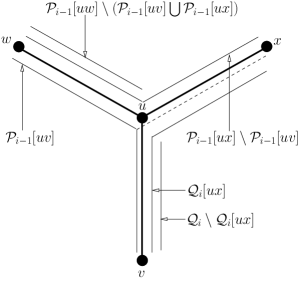
Figure 1: Sets of interesting rooted subtrees encountered while processing edge $\{u,v\}$ of type $4$ defined in Lemma 3.3. Solid line on an edge implies that every rooted subtree of that set must be present on that edge. Absence of a line on an edge implies that no rooted subtree of that set can be present on that edge. Dotted line on an edge implies that rooted subtrees of the set may or may not be present on that edge.

Lemma 3.6

If edge $e_{i}=\{u,v\}$ being processed in the $i$-th round of GREEDY-COL is of type $4$ defined in Lemma 3.3, then

$$|\psi^{\mathrm{GDY}}(\mathcal{P}_{i})| =\max\Big{\{}\big{|}\psi^{\mathrm{GDY}}(\mathcal{Q}_{i}\cup\mathcal{P}_{i-1}[\{u,w\}])\big{|},$$

$$\phantom{=\max\Big{\{}}|\psi^{\mathrm{GDY}}(\mathcal{P}_{i-1})|\Big{\}},$$

where the edge $\{u,w\}\in E_{T}$ is as defined in Lemma 3.3.

• Since the edge $e_{i}=\{u,v\}$ being processed in the $i$-th round of coloring is of type $4$ defined in Lemma 3.3, according to Lemma 3.4, if a rooted subtree that has already been colored in the first $i-1$ rounds of GREEDY-COL collides with any rooted subtree that is to be colored in the $i$-th round, then it must belong to the set $\mathcal{P}_{i-1}[\{u,v\}]\cup\mathcal{P}_{i-1}[\{u,x\}]$. Since $\mathcal{P}_{i-1}[\{u,v\}]\cup\mathcal{P}_{i-1}[\{u,x\}]\subseteq\mathcal{P}_{i-1}[\{u,w\}]$, this implies that any rooted subtree in the set $\mathcal{P}_{i-1}\setminus\mathcal{P}_{i-1}[\{u,w\}]$ cannot collide with any rooted subtree in the set $\mathcal{Q}_{i}$. Therefore, any color already assigned to some rooted subtree in the set $\mathcal{P}_{i-1}\setminus\mathcal{P}_{i-1}[\{u,w\}]$, but not to any rooted subtree in the set $\mathcal{P}_{i-1}[\{u,w\}]$, can be assigned to any rooted subtree in the set $\mathcal{Q}_{i}$. There are $|\psi^{\mathrm{GDY}}(\mathcal{P}_{i-1})|-|\psi^{\mathrm{GDY}}(\mathcal{P}_{i-1}[\{u,w\}])|$ such colors. During the $i$-th round of coloring, let $\mathcal{N}_{i}\subseteq\mathcal{Q}_{i}$ be the set of rooted subtrees which do not share colors with rooted subtrees in the set $\mathcal{P}_{i-1}[\{u,w\}]$, i.e, $\mathcal{Q}_{i}\setminus\mathcal{N}_{i}$ is the largest subset of the set $\mathcal{Q}_{i}$ such that $|\psi^{\mathrm{GDY}}(\left(\mathcal{Q}_{i}\setminus\mathcal{N}_{i}\right)\cup\mathcal{P}_{i-1}[\{u,w\}])|=|\psi^{\mathrm{GDY}}(\mathcal{P}_{i-1}[\{u,w\}])|$. We need $|\psi^{\mathrm{GDY}}(\mathcal{N}_{i})|$ additional colors for coloring all the rooted subtrees in the set $\mathcal{N}_{i}$ and there are $|\psi^{\mathrm{GDY}}(\mathcal{P}_{i-1})|-|\psi^{\mathrm{GDY}}(\mathcal{P}_{i-1}[\{u,w\}])|$ available colors that can be used without adding any new color in the $i$-th round of coloring. Therefore, the total number of colors required at the end of $i$-th round of coloring in GREEDY-COL is

  $$|\psi^{\mathrm{GDY}}(\mathcal{P}_{i})|$$

  $$= \bigg{[}|\psi^{\mathrm{GDY}}(\mathcal{N}_{i})|-\Big{(}|\psi^{\mathrm{GDY}}(\mathcal{P}_{i-1})|$$

  $${}-|\psi^{\mathrm{GDY}}(\mathcal{P}_{i-1}[\{u,w\}])|\Big{)}\bigg{]}^{+}+|\psi^{\mathrm{GDY}}(\mathcal{P}_{i-1})|$$

  $$= \Big{[}|\psi^{\mathrm{GDY}}(\mathcal{N}_{i})|+\big{|}\psi^{\mathrm{GDY}}(\left(\mathcal{Q}_{i}\setminus\mathcal{N}_{i}\right)\cup\mathcal{P}_{i-1}[\{u,w\}])\big{|}$$

  $${}-|\psi^{\mathrm{GDY}}(\mathcal{P}_{i-1})|\Big{]}^{+}+|\psi^{\mathrm{GDY}}(\mathcal{P}_{i-1})|$$

  $$= \Big{[}\big{|}\psi^{\mathrm{GDY}}(\mathcal{Q}_{i}\cup\mathcal{P}_{i-1}[\{u,w\}])\big{|}-|\psi^{\mathrm{GDY}}(\mathcal{P}_{i-1})|\Big{]}^{+}$$

  $${}+|\psi^{\mathrm{GDY}}(\mathcal{P}_{i-1})|$$

  $$= \max\left\{\big{|}\psi^{\mathrm{GDY}}(\mathcal{Q}_{i}\cup\mathcal{P}_{i-1}[\{u,w\}])\big{|},|\psi^{\mathrm{GDY}}(\mathcal{P}_{i-1})|\right\},$$

  where the third equality is due to the fact that the rooted subtrees in the set $\mathcal{N}_{i}$ do not share any color with the rooted subtrees in the set $\left(\mathcal{Q}_{i}\setminus\mathcal{N}_{i}\right)\cup\mathcal{P}_{i-1}[\{u,w\}]$.

Lemma 3.6 suggests that we should develop bounds for $|\psi^{\mathrm{GDY}}(\mathcal{Q}_{i}\cup\mathcal{P}_{i-1}[\{u,w\}])|$. Using the notation of the lemma, if $\mathcal{N}_{i}\subseteq\mathcal{Q}_{i}$ is the set of rooted subtrees that do not share colors with any rooted subtrees in the set $\mathcal{P}_{i-1}[\{u,w\}]$, then

$$\big{|}\psi^{\mathrm{GDY}}(\mathcal{Q}_{i}\cup\mathcal{P}_{i-1}[\{u,w\}])\big{|}$$

$$= |\psi^{\mathrm{GDY}}(\mathcal{N}_{i})|+\big{|}\psi^{\mathrm{GDY}}(\left(\mathcal{Q}_{i}\setminus\mathcal{N}_{i}\right)\cup\mathcal{P}_{i-1}[\{u,w\}])\big{|}$$

$$= |\psi^{\mathrm{GDY}}(\mathcal{N}_{i})|+|\psi^{\mathrm{GDY}}(\mathcal{P}_{i-1}[\{u,w\}])|.$$

Hence, in order to limit the use of new colors in the $i$-th round of coloring, we try to minimize $|\psi^{\mathrm{GDY}}(\mathcal{N}_{i})|$, the number of colors used in the $i$-th round of coloring that are different from the colors assigned to the rooted subtrees in the set $\mathcal{P}_{i-1}[\{u,w\}]$.

For any set $\mathcal{S}$ of rooted subtrees on the given host tree $T$ such that the complement of their conflict graph is bipartite, i.e., $\bar{G}_{\mathcal{S}}$ is bipartite, we denote the size of maximum matching [3, p.67] in $\bar{G}_{\mathcal{S}}$ by $m_{\mathcal{S}}$.

Lemma 3.7

If the edge $e_{i}=\{u,v\}$ is of type $4$ defined in Lemma 3.3, and PROCESS-EDGE-1 is used for coloring in the $i$-th round of GREEDY-COL, then

$$\big{|}\psi^{\mathrm{GDY}}(\mathcal{Q}_{i}\cup\mathcal{P}_{i-1}[\{u,w\}])\big{|}$$

$$\leq 2l_{\mathcal{R}}+|\mathcal{Q}_{i}|-m_{\mathcal{R}[\{u,v\}]}+m_{\mathcal{P}_{i-1}[\{u,v\}]}.$$

• In order to limit $|\psi^{\mathrm{GDY}}(\mathcal{P}_{i-1}[\{u,w\}]\cup\mathcal{Q}_{i})|-|\psi^{\mathrm{GDY}}(\mathcal{P}_{i-1}[\{u,w\}])|$, PROCESS-EDGE-1 finds the maximum number of disjoint pairs $\vec{R},\vec{S}$ of rooted subtrees such that one of the following is true:

  • Both $\vec{R},\vec{S}\in\mathcal{Q}_{i}$, and in this case they are assigned the same (possibly new) color.

  • $\vec{R}\in\mathcal{Q}_{i},\vec{S}\in\mathcal{P}_{i-1}[\{u,v\}]$, and in this case $\vec{R}$ is assigned the same color as $\vec{S}$.

  PROCESS-EDGE-1 finds such pairs of rooted subtrees by using graph $B_{1}$. Since $\mathcal{P}_{i-1}[\{u,v\}]$ and $\mathcal{Q}_{i}$ partition the set $\mathcal{R}[\{u,v\}]$, therefore by Lemma 3.1, graph $\bar{G}_{\mathcal{P}_{i-1}[\{u,v\}]\cup\mathcal{Q}_{i}}$ is bipartite. This, along with the fact that $E_{G_{\mathcal{P}_{i-1}[\{u,v\}]\cup\mathcal{Q}_{i}}}\subseteq E_{B_{1}}$, implies that $\bar{B}_{1}$ is also bipartite. Hence, it is easy to find a maximum matching in $\bar{B}_{1}$. Let $M\subseteq E_{\bar{B}_{1}}$ be any matching in $\bar{B}_{1}$. Observe that the edges are added to $B_{1}$ (lines 2-6) in such a way that if edge $\{\vec{R},\vec{S}\}\in M$, then one of the following holds:

  • Both $\vec{R},\vec{S}\in\mathcal{Q}_{i}$.

  • $\vec{R}\in\mathcal{P}_{i-1},\vec{S}\in\mathcal{Q}_{i}$, and there is no $\vec{U}\in\mathcal{P}_{i-1}$ such that $\vec{S},\vec{U}$ collide and $\psi^{\mathrm{GDY}}(\vec{R})=\psi^{\mathrm{GDY}}(\vec{U})$.

  • Both $\vec{R},\vec{S}\in\mathcal{P}_{i-1}$ and $\psi^{\mathrm{GDY}}(\vec{R})=\psi^{\mathrm{GDY}}(\vec{S})$.

  So if edge $\{\vec{R},\vec{S}\}\in M$, then rooted subtrees $\vec{R}$ and $\vec{S}$ can be assigned the same color. Note that the matched edges of type (i) and (ii) correspond to the rooted subtree pairs of type (i) and (ii), respectively. Matched edges of type (iii) simply list all the pairs of rooted subtrees in the set $\mathcal{P}_{i-1}[\{u,v\}]$ that have already been assigned the same colors. Since the number of edges of type (iii) is already fixed, a maximum matching in $\bar{B}_{1}$ determines the maximum number of edges of types (i) and (ii), i.e., it determines the maximum number of rooted subtree pairs described above.

  First assume that the rooted subtrees in the set $\mathcal{P}_{i-1}[\{u,v\}]$ do not share colors with any of the rooted subtree in the set $\mathcal{P}_{i-1}[\{u,w\}]\setminus\mathcal{P}_{i-1}[\{u,v\}]$, although they may share colors amongst themselves. As a consequence of Lemma 3.1, more than two rooted subtrees in the set $\mathcal{P}_{i-1}[\{u,v\}]$ cannot have the same color. Starting from any maximum matching $M_{\bar{G}_{\mathcal{P}_{i-1}[\{u,v\}]\cup\mathcal{Q}_{i}}}\subseteq E_{\bar{G}_{\mathcal{P}_{i-1}[\{u,v\}]\cup\mathcal{Q}_{i}}}$ in graph $\bar{G}_{\mathcal{P}_{i-1}[\{u,v\}]\cup\mathcal{Q}_{i}}$, we can construct a matching $M\subseteq E_{\bar{B}_{1}}$ in graph $\bar{B}_{1}$ by first removing and then adding the edges described next. We remove every matched edge $\{\vec{R},\vec{S}\}\in M_{\bar{G}_{\mathcal{P}_{i-1}[\{u,v\}]\cup\mathcal{Q}_{i}}}$ for which one of the following is true:

  • Both $\vec{R},\vec{S}\in\mathcal{P}_{i-1}[\{u,v\}]$ such that $\psi^{\mathrm{GDY}}(\vec{R})\neq\psi^{\mathrm{GDY}}(\vec{S})$, and there is no rooted subtree $\vec{U}\in\mathcal{P}_{i-1}[\{u,v\}]$ such that $\psi^{\mathrm{GDY}}(\vec{U})\notin\{\psi^{\mathrm{GDY}}(\vec{R}),\psi^{\mathrm{GDY}}(\vec{S})\}$.

  • Both $\vec{R},\vec{S}\in\mathcal{P}_{i-1}[\{u,v\}]$ such that $\psi^{\mathrm{GDY}}(\vec{R})\neq\psi^{\mathrm{GDY}}(\vec{S})$, and there is a rooted subtree $\vec{U}\in\mathcal{P}_{i-1}[\{u,v\}]$ such that $\psi^{\mathrm{GDY}}(\vec{U})\in\{\psi^{\mathrm{GDY}}(\vec{R}),\psi^{\mathrm{GDY}}(\vec{S})\}$.

  • $\vec{R}\in\mathcal{Q}_{i}$, $\vec{S}\in\mathcal{P}_{i-1}[\{u,v\}]$, and there is a rooted subtree $\vec{U}\in\mathcal{P}_{i-1}$ such that $\psi^{\mathrm{GDY}}(\vec{U})=\psi^{\mathrm{GDY}}(\vec{S})$.

  Consider rooted subtrees $\vec{R},\vec{S}\in\mathcal{P}_{i-1}[\{u,v\}]$ with $\psi^{\mathrm{GDY}}(\vec{R})=\psi^{\mathrm{GDY}}(\vec{S})$. Since $M_{\bar{G}_{\mathcal{P}_{i-1}[\{u,v\}]\cup\mathcal{Q}_{i}}}$ is a maximum matching in $\bar{G}_{\mathcal{P}_{i-1}[\{u,v\}]\cup\mathcal{Q}_{i}}$, either edge $\{\vec{R},\vec{S}\}\in M_{\bar{G}_{\mathcal{P}_{i-1}[\{u,v\}]\cup\mathcal{Q}_{i}}}$, or at least one of the rooted subtrees $\vec{R},\vec{S}$ is matched to some other rooted subtree in $M_{\bar{G}_{\mathcal{P}_{i-1}[\{u,v\}]\cup\mathcal{Q}_{i}}}$. In the case when rooted subtrees $\vec{R},\vec{S}$ are not already matched to each other in $M_{\bar{G}_{\mathcal{P}_{i-1}[\{u,v\}]\cup\mathcal{Q}_{i}}}$, the edge(s) adjacent to $\vec{R}$ or $\vec{S}$ (or both) in $M_{\bar{G}_{\mathcal{P}_{i-1}[\{u,v\}]\cup\mathcal{Q}_{i}}}$ is (are) either of type (ii) or of type (iii) and is (are) therefore removed from the matching. Hence, we can safely add edge $\{\vec{R},\vec{S}\}$ to the matching. Let the set of removed edges of type (i), (ii) and (iii) be $E_{\mathrm{r(i)}}$, $E_{\mathrm{r(ii)}}$ and $E_{\mathrm{r(iii)}}$, respectively, and the set of added edges be $E_{\mathrm{a}}$. Observe that for every removed edge in the set $E_{\mathrm{r(ii)}}\cup E_{\mathrm{r(iii)}}$, there is a corresponding edge in the set $E_{\mathrm{a}}$ added to the matching such that for at most two removed edges in the set $E_{\mathrm{r(ii)}}\cup E_{\mathrm{r(iii)}}$, the corresponding added edge in the set $E_{\mathrm{a}}$ can be the same; therefore $|E_{\mathrm{a}}|\geq\frac{1}{2}(|E_{\mathrm{r(ii)}}|+|E_{\mathrm{r(iii)}}|)$. We can now lower bound the size of maximum matching $M_{\bar{B}_{1}}\subseteq E_{\bar{B}_{1}}$ in graph $\bar{B}_{1}$ by the size of $M$, a valid matching in the graph. $|M|$ is equal to $|M_{\bar{G}_{\mathcal{P}_{i-1}[\{u,v\}]\cup\mathcal{Q}_{i}}}|=m_{\{T\mathcal{P}_{i-1}[\{u,v\}]\cup\mathcal{Q}_{i}\}}$ minus the number of edges removed plus the number of edges added. Thus

  (3.3) $$|M_{\bar{B}_{1}}|\geq|M|$$

  $$= m_{\mathcal{P}_{i-1}[\{u,v\}]\cup\mathcal{Q}_{i}}-\left(|E_{\mathrm{r(i)}}|+|E_{\mathrm{r(ii)}}|+|E_{\mathrm{r(iii)}}|-|E_{\mathrm{a}}|\right)$$

  $$\geq m_{\mathcal{P}_{i-1}[\{u,v\}]\cup\mathcal{Q}_{i}}-\left(|E_{\mathrm{r(i)}}|+|E_{\mathrm{a}}|\right)$$

  $$\geq m_{\mathcal{P}_{i-1}[\{u,v\}]\cup\mathcal{Q}_{i}}-m_{\mathcal{P}_{i-1}[\{u,v\}]},$$

  where we are using the fact that $E_{\mathrm{a}}\cup E_{\mathrm{r(i)}}$, the set of removed edges of type (i) and the set of added edges form a matching in the bipartite graph $\bar{G}_{\mathcal{P}_{i-1}[\{u,v\}]}$. This is because $E_{\mathrm{a}}\cup E_{\mathrm{r(i)}}\subseteq E_{\bar{G}_{\mathcal{P}_{i-1}[\{u,v\}]}}$, and the end vertices of edges in the sets $E_{\mathrm{a}},E_{\mathrm{r(i)}}$ are distinct.

  The vertex set $V_{\bar{B}_{1}}$ corresponds to all the rooted subtrees in the set $\mathcal{P}_{i-1}[\{u,v\}]\cup\mathcal{Q}_{i}$, and an edge in matching $M_{\bar{B}_{1}}$ determines two rooted subtrees which share their color after this round of coloring. Therefore, using inequality (3.3) and the fact that the subsets $\mathcal{P}_{i-1}[\{u,v\}]$ and $\mathcal{Q}_{i}$ partition the set $\mathcal{R}[\{u,v\}]$,

  (3.4) $$\big{|}\psi^{\mathrm{GDY}}(\mathcal{P}_{i-1}[\{u,v\}]\cup\mathcal{Q}_{i})\big{|}$$

  $$\leq \big{|}\mathcal{P}_{i-1}[\{u,v\}]\cup\mathcal{Q}_{i}\big{|}-|M_{\bar{B}_{1}}|$$

  $$\leq |\mathcal{P}_{i-1}[\{u,v\}]|+|\mathcal{Q}_{i}|-m_{\mathcal{P}_{i-1}[\{u,v\}]\cup\mathcal{Q}_{i}}+m_{\mathcal{P}_{i-1}[\{u,v\}]}.$$

  Using inequality (3.4)

  (3.5) $$\big{|}\psi^{\mathrm{GDY}}(\mathcal{P}_{i-1}[\{u,w\}]\cup\mathcal{Q}_{i})\big{|}$$

  $$= \big{|}\psi^{\mathrm{GDY}}(\mathcal{P}_{i-1}[\{u,w\}]\cup\mathcal{Q}_{i})\big{|}-\big{|}\psi^{\mathrm{GDY}}(\mathcal{P}_{i-1}[\{u,v\}]\cup\mathcal{Q}_{i})\big{|}$$

  $${}+\big{|}\psi^{\mathrm{GDY}}(\mathcal{P}_{i-1}[\{u,v\}]\cup\mathcal{Q}_{i})\big{|}$$

  $$\leq |\mathcal{P}_{i-1}[\{u,w\}]\setminus\mathcal{P}_{i-1}[\{u,v\}]|+|\mathcal{P}_{i-1}[\{u,v\}]|+|\mathcal{Q}_{i}|$$

  $${}-m_{\mathcal{P}_{i-1}[\{u,v\}]\cup\mathcal{Q}_{i}}+m_{\mathcal{P}_{i-1}[\{u,v\}]}$$

  $$\leq 2l_{\mathcal{R}}+|\mathcal{Q}_{i}|-m_{\mathcal{R}[\{u,v\}]}+m_{\mathcal{P}_{i-1}[\{u,v\}]}.$$

  The first inequality uses the fact that $|\psi^{\mathrm{GDY}}(\mathcal{P}_{i-1}[\{u,w\}]\cup\mathcal{Q}_{i})|-|\psi^{\mathrm{GDY}}(\mathcal{P}_{i-1}[\{u,v\}]\cup\mathcal{Q}_{i})|$ is the number of colors used for coloring all the rooted subtrees in the set $\mathcal{P}_{i-1}[\{u,w\}]\setminus\mathcal{P}_{i-1}[\{u,v\}]$ that are different from the colors used for coloring rooted subtrees in the set $\mathcal{P}_{i-1}[\{u,v\}]\cup\mathcal{Q}_{i}$; therefore, this number is upper bounded by $|\mathcal{P}_{i-1}[\{u,w\}]\setminus\mathcal{P}_{i-1}[\{u,v\}]|$. The final inequality uses the fact that the subsets $\mathcal{P}_{i-1}[\{u,v\}]$ and $\mathcal{P}_{i-1}[\{u,w\}]\setminus\mathcal{P}_{i-1}[\{u,v\}]$ partition the set $\mathcal{P}_{i-1}[\{u,w\}]=\mathcal{R}[\{u,w\}]$.

  Next, suppose some rooted subtree $\vec{R}\in\mathcal{P}_{i-1}[\{u,v\}]$ shares its color with another rooted subtree $\vec{S}\in\mathcal{P}_{i-1}[\{u,w\}]\setminus\mathcal{P}_{i-1}[\{u,v\}]$. In this case, the worst that can happen is that some rooted subtrees in the set $\mathcal{Q}_{i}$, that could have shared color with rooted subtree $\vec{R}$, can no longer do so since they collide with rooted subtree $\vec{S}$. Hence the size of maximum matching $M_{\bar{B}_{1}}$ reduces by $1$. The unit reduction is independent of the number of affected rooted subtrees in the set $\mathcal{Q}_{i}$, since in $M_{\bar{B}_{1}}$ rooted subtree $\vec{R}$ can be potentially matched to only one of them. On the other hand, the rooted subtrees $\vec{R}\in\mathcal{P}_{i-1}[\{u,v\}],\vec{S}\in\mathcal{P}_{i-1}[\{u,w\}]\setminus\mathcal{P}_{i-1}[\{u,v\}]$ sharing color means that $|\psi^{\mathrm{GDY}}(\mathcal{P}_{i-1}[\{u,w\}]\cup\mathcal{Q}_{i})|-|\psi^{\mathrm{GDY}}(\mathcal{P}_{i-1}[\{u,v\}]\cup\mathcal{Q}_{i})|$, the number of colors used for assigning colors to all the rooted subtrees in the set $\mathcal{P}_{i-1}[\{u,w\}]\setminus\mathcal{P}_{i-1}[\{u,v\}]$ that are different from the colors used for assigning colors to the rooted subtrees in the set $\mathcal{P}_{i-1}[\{u,v\}]\cup\mathcal{Q}_{i}$, also reduces by $1$. Applying both the observations, we note that the final inequality in (3.5) still holds.

Lemma 3.8

If the edge $e_{i}=\{u,v\}$ is of type $4$ defined in Lemma 3.3, and PROCESS-EDGE-2 is used for coloring in the $i$-th round of GREEDY-COL, then

$$\big{|}\psi^{\mathrm{GDY}}(\mathcal{P}_{i-1}[\{u,w\}]\cup\mathcal{Q}_{i})\big{|}\leq 2l_{\{\vec{T}_{H},\mathcal{R}\}}+\left[g-h\right]^{+},$$

where

$$g= |\mathcal{Q}_{i}[\{u,x\}]|+|\mathcal{P}_{i-1}[\{u,x\}]\setminus\mathcal{P}_{i-1}[\{u,v\}]|-|\mathcal{Q}_{i}|,$$

$$h= \Bigg{[}|\mathcal{Q}_{i}[\{u,x\}]|+\frac{|\mathcal{P}_{i-1}[\{u,x\}]\setminus\mathcal{P}_{i-1}[\{u,v\}]|}{2}$$

$${}+m_{\mathcal{R}[\{u,x\}]}-2l_{\mathcal{R}}\Bigg{]}^{+}.$$

• Observe that $\mathcal{P}_{i-1}[\{u,v\}]$ and $\mathcal{P}_{i-1}[\{u,w\}]\setminus\mathcal{P}_{i-1}[\{u,v\}]$ partition $\mathcal{P}_{i-1}[\{u,w\}]=\mathcal{R}[\{u,w\}]$, and $\mathcal{P}_{i-1}[\{u,v\}]$ and $\mathcal{Q}_{i}$ partition $\mathcal{R}[\{u,v\}]$. Since $|\mathcal{R}[\{u,w\}]|=|\mathcal{R}[\{u,v\}]|=2l_{\mathcal{R}}$, we have

  (3.6) $$|\mathcal{P}_{i-1}[\{u,w\}]\setminus\mathcal{P}_{i-1}[\{u,v\}]|=|\mathcal{Q}_{i}|.$$

  Since $\mathcal{Q}_{i}[\{u,x\}]$ and $\mathcal{Q}_{i}\setminus\mathcal{Q}_{i}[\{u,x\}]$ partition $\mathcal{Q}_{i}$, and $\mathcal{P}_{i-1}[\{u,x\}]\setminus\mathcal{P}_{i-1}[\{u,v\}]$ and $\mathcal{P}_{i-1}[\{u,w\}]\setminus\left(\mathcal{P}_{i-1}[\{u,v\}]\cup\mathcal{P}_{i-1}[\{u,x\}]\right)$ partition $\mathcal{P}_{i-1}[\{u,w\}]\setminus\mathcal{P}_{i-1}[\{u,v\}]$, from equation (3.6)

  (3.7) $$\big{|}\mathcal{P}_{i-1}[\{u,w\}]\setminus\left(\mathcal{P}_{i-1}[\{u,v\}]\cup\mathcal{P}_{i-1}[\{u,x\}]\right)\big{|}$$

  $${}+|\mathcal{P}_{i-1}[\{u,x\}]\setminus\mathcal{P}_{i-1}[\{u,v\}]|$$

  $$= |\mathcal{P}_{i-1}[\{u,w\}]\setminus\mathcal{P}_{i-1}[\{u,v\}]|$$

  $$= |\mathcal{Q}_{i}\setminus\mathcal{Q}_{i}[\{u,x\}]|+|\mathcal{Q}_{i}[\{u,x\}]|=|\mathcal{Q}_{i}|.$$

  PROCESS-EDGE-2 first finds the maximum number of disjoint pairs $\vec{R},\vec{S}$ of rooted subtrees such that one of the following is true:

  • Both $\vec{R},\vec{S}\in\mathcal{Q}_{i}[\{u,x\}]$. In this case, both $\vec{R}$ and $\vec{S}$ are assigned the same color (we shall specify exactly which color is assigned in a moment).

  • $\vec{R}\in\mathcal{Q}_{i}[\{u,x\}]$ and $\vec{S}\in\mathcal{P}_{i-1}[\{u,x\}]\setminus\mathcal{P}_{i-1}[\{u,v\}]$ such that $\vec{R}$ can be assigned the same color as $\vec{S}$. In this case $\vec{R}$ is indeed assigned the same color as $\vec{S}$.

  PROCESS-EDGE-2 finds such pairs of rooted subtrees by using graph $B_{2}$. Since $\mathcal{P}_{i-1}[\{u,x\}]\setminus\mathcal{P}_{i-1}[\{u,v\}]$ and $\mathcal{Q}_{i}[\{u,x\}]$ are disjoint subsets of $\mathcal{R}[\{u,x\}]$, by Lemma 3.1 the graph $\bar{G}_{(\mathcal{P}_{i-1}[\{u,x\}]\setminus\mathcal{P}_{i-1}[\{u,v\}])\cup\mathcal{Q}_{i}[\{u,x\}]}$ is bipartite. This, along with the fact that $E_{G_{(\mathcal{P}_{i-1}[\{u,x\}]\setminus\mathcal{P}_{i-1}[\{u,v\}])\cup\mathcal{Q}_{i}[\{u,x\}]}}\subseteq E_{B_{2}}$, implies that $\bar{B}_{2}$ is also bipartite. Hence, it is easy to find a maximum matching in $\bar{B}_{2}$. Let $M\subseteq E_{\bar{B}_{2}}$ be any matching in $\bar{B}_{2}$. Edges are added to $B_{2}$ in such a way that if edge $\{\vec{R},\vec{S}\}\in M$, then one of the following holds:

  • Both $\vec{R},\vec{S}\in\mathcal{Q}_{i}[\{u,x\}]$.

  • $\vec{R}\in\mathcal{Q}_{i}[\{u,x\}],\vec{S}\in\mathcal{P}_{i-1}[\{u,x\}]\setminus\mathcal{P}_{i-1}[\{u,v\}]$, and there is no $\vec{U}\in\mathcal{P}_{i-1}$ such that $\vec{R},\vec{U}$ collide and $\psi^{\mathrm{GDY}}(\vec{S})=\psi^{\mathrm{GDY}}(\vec{U})$.

  • Both $\vec{R},\vec{S}\in\mathcal{P}_{i-1}[\{u,x\}]\setminus\mathcal{P}_{i-1}[\{u,v\}]$ and $\psi^{\mathrm{GDY}}(\vec{R})=\psi^{\mathrm{GDY}}(\vec{S})$.

  So if edge $\{\vec{R},\vec{S}\}\in M$, then the rooted subtrees $\vec{R},\vec{S}$ can be assigned the same color. Note that the matched edges of type (i) and (ii) correspond to the rooted subtree pairs of type (i) and (ii), respectively. Matched edges of type (iii) simply list all the pairs of rooted subtrees in the set $\mathcal{P}_{i-1}[\{u,x\}]\setminus\mathcal{P}_{i-1}[\{u,v\}]$ that have already been colored. Since the number of edges of type (iii) is already fixed, a maximum matching in $\bar{B}_{2}$ determines the maximum number of edges of types (i) and (ii), i.e., it determines the maximum number of rooted subtree pairs described above.

  First, we assume that the rooted subtrees in the set $\mathcal{P}_{i-1}[\{u,w\}]\setminus\mathcal{P}_{i-1}[\{u,v\}]$ do not share colors with any rooted subtree in the set $\mathcal{P}_{i-1}[\{u,v\}]$, although they may share colors amongst themselves. Let $M_{\bar{B}_{2}}\subseteq E_{\bar{B}_{2}}$ be a maximum matching in $\bar{B}_{2}$. Let the number of type (i), (ii) and (iii) edges in the matching be $t_{1},t_{2},t_{3}$, respectively. In this case the size of the maximum matching in $\bar{B}_{2}$ is lower bounded as

  (3.8) $$|M_{\bar{B}_{2}}|=\sum_{j=1}^{3}t_{j}$$

  $$\geq m_{\mathcal{Q}_{i}[\{u,x\}]\cup\left(\mathcal{P}_{i-1}[\{u,x\}]\setminus\mathcal{P}_{i-1}[\{u,v\}]\right)}$$

  $${}-m_{\mathcal{P}_{i-1}[\{u,x\}]\setminus\mathcal{P}_{i-1}[\{u,v\}]}$$

  $$\geq \bigg{[}m_{\mathcal{Q}_{i}[\{u,x\}]\cup\left(\mathcal{P}_{i-1}[\{u,x\}]\setminus\mathcal{P}_{i-1}[\{u,v\}]\right)}$$

  $${}-\frac{|\mathcal{P}_{i-1}[\{u,x\}]\setminus\mathcal{P}_{i-1}[\{u,v\}]|}{2}\bigg{]}^{+},$$

  where $m_{\mathcal{Q}_{i}[\{u,x\}]\cup\left(\mathcal{P}_{i-1}[\{u,x\}]\setminus\mathcal{P}_{i-1}[\{u,v\}]\right)}$ and $m_{\mathcal{P}_{i-1}[\{u,x\}]\setminus\mathcal{P}_{i-1}[\{u,v\}]}$ are the sizes of maximum matchings in the bipartite graphs $\bar{G}_{\mathcal{Q}_{i}[\{u,x\}]\cup\left(\mathcal{P}_{i-1}[\{u,x\}]\setminus\mathcal{P}_{i-1}[\{u,v\}]\right)}$ and $\bar{G}_{\mathcal{P}_{i-1}[\{u,x\}]\setminus\mathcal{P}_{i-1}[\{u,v\}]}$, respectively. The reasoning for the initial inequality follows exactly as the reasoning for inequality (3.3) presented in the proof of Lemma 3.7. For the final inequality, we use the facts that the size of any matching in the bipartite graph $\bar{G}_{\mathcal{P}_{i-1}[\{u,x\}]\setminus\mathcal{P}_{i-1}[\{u,v\}]}$ must be smaller than half of the size of its vertex set, and the size of a matching cannot be negative. Since $\bar{G}_{\mathcal{Q}_{i}[\{u,x\}]\cup\left(\mathcal{P}_{i-1}[\{u,x\}]\setminus\mathcal{P}_{i-1}[\{u,v\}]\right)}$ is a subgraph of $\bar{G}_{\mathcal{R}[\{u,x\}]}$ induced by the vertex set corresponding to the rooted subtrees in the set $\mathcal{Q}_{i}[\{u,x\}]\cup\left(\mathcal{P}_{i-1}[\{u,x\}]\setminus\mathcal{P}_{i-1}[\{u,v\}]\right)$, if the size of a maximum matching in $\bar{G}_{\mathcal{R}[\{u,x\}]}$ is $m_{\mathcal{R}[\{u,x\}]}$, then the size of a maximum matching in $\bar{G}_{\mathcal{Q}_{i}[\{u,x\}]\cup\left(\mathcal{P}_{i-1}[\{u,x\}]\setminus\mathcal{P}_{i-1}[\{u,v\}]\right)}$ is bounded as

  (3.9) $$m_{\mathcal{Q}_{i}[\{u,x\}]\cup\left(\mathcal{P}_{i-1}[\{u,x\}]\setminus\mathcal{P}_{i-1}[\{u,v\}]\right)}$$

  $$\geq \bigg{[}m_{\mathcal{R}[\{u,x\}]}-|\mathcal{R}[\{u,x\}]|+\big{|}\mathcal{Q}_{i}[\{u,x\}]\cup$$

  $$\Big{(}\mathcal{P}_{i-1}[\{u,x\}]\setminus\mathcal{P}_{i-1}[\{u,v\}]\Big{)}\big{|}\bigg{]}^{+}$$

  $$= \bigg{[}|\mathcal{Q}_{i}[\{u,x\}]|+|\mathcal{P}_{i-1}[\{u,x\}]\setminus\mathcal{P}_{i-1}[\{u,v\}]|$$

  $${}+m_{\mathcal{R}[\{u,x\}]}-2l_{\mathcal{R}}\bigg{]}^{+}.$$

  This is because if we consider a maximum matching $M_{\bar{G}_{\mathcal{R}[\{u,x\}]}}\subseteq E_{\bar{G}_{\mathcal{R}[\{u,x\}]}}$ in the graph $\bar{G}_{\mathcal{R}[\{u,x\}]}$, any edge $\{\vec{R},\vec{S}\}\in M_{\bar{G}_{\mathcal{R}[\{u,x\}]}}$ can be classified into one of the following three types:

  • Both $\vec{R},\vec{S}\in\mathcal{Q}_{i}[\{u,x\}]\cup\left(\mathcal{P}_{i-1}[\{u,x\}]\setminus\mathcal{P}_{i-1}[\{u,v\}]\right)$.

  • Rooted subtree $\vec{R}\in\mathcal{Q}_{i}[\{u,x\}]\cup\left(\mathcal{P}_{i-1}[\{u,x\}]\setminus\mathcal{P}_{i-1}[\{u,v\}]\right)$ whereas rooted subtree $\vec{S}\in\mathcal{R}[\{u,x\}]\setminus\left(\mathcal{Q}_{i}[\{u,x\}]\cup\left(\mathcal{P}_{i-1}[\{u,x\}]\setminus\mathcal{P}_{i-1}[\{u,v\}]\right)\right)$.

  • Both $\vec{R},\vec{S}\in\mathcal{R}[\{u,x\}]\setminus\left(\mathcal{Q}_{i}[\{u,x\}]\cup\left(\mathcal{P}_{i-1}[\{u,x\}]\setminus\mathcal{P}_{i-1}[\{u,v\}]\right)\right)$.

  Let the set of edges of type (i), (ii) and (iii) be $E_{\mathrm{(i)}},E_{\mathrm{(ii)}},E_{\mathrm{(iii)}}$, respectively. Clearly, $E_{\mathrm{(i)}}$ is a valid matching in the graph $\bar{G}_{\mathcal{Q}_{i}[\{u,x\}]\cup\left(\mathcal{P}_{i-1}[\{u,x\}]\setminus\mathcal{P}_{i-1}[\{u,v\}]\right)}$, therefore a lower bound for $|E_{\mathrm{(i)}}|$ can be treated as a lower bound for $m_{\mathcal{Q}_{i}[\{u,x\}]\cup\left(\mathcal{P}_{i-1}[\{u,x\}]\setminus\mathcal{P}_{i-1}[\{u,v\}]\right)}$. Also, since maximum matching $M_{\bar{G}_{\mathcal{R}[\{u,x\}]}}$ can be partitioned into sets $E_{\mathrm{(i)}},E_{\mathrm{(ii)}},E_{\mathrm{(iii)}}$, we get

  (3.10) $$m_{\mathcal{Q}_{i}[\{u,x\}]\cup\left(\mathcal{P}_{i-1}[\{u,x\}]\setminus\mathcal{P}_{i-1}[\{u,v\}]\right)}$$

  $$\geq |E_{\mathrm{(i)}}|\geq m_{\mathcal{R}[\{u,x\}]}-|E_{\mathrm{(ii)}}|-|E_{\mathrm{(iii)}}|.$$

  Since an edge in the set $E_{\mathrm{(ii)}}$ requires one of the rooted subtree, and an edge in the set $E_{\mathrm{(iii)}}$ requires both of the rooted subtrees to be from the set $\mathcal{R}[\{u,x\}]\setminus\left(\mathcal{Q}_{i}[\{u,x\}]\cup\left(\mathcal{P}_{i-1}[\{u,x\}]\setminus\mathcal{P}_{i-1}[\{u,v\}]\right)\right)$, we have

  (3.11) $$\qquad\qquad|E_{\mathrm{(ii)}}|+2|E_{\mathrm{(iii)}}|$$

  $$\leq \big{|}\mathcal{R}[\{u,x\}]\setminus\left(\mathcal{Q}_{i}[\{u,x\}]\cup\left(\mathcal{P}_{i-1}[\{u,x\}]\setminus\mathcal{P}_{i-1}[\{u,v\}]\right)\right)\big{|}$$

  $$= |\mathcal{R}[\{u,x\}]|-\big{|}\mathcal{Q}_{i}[\{u,x\}]\cup\left(\mathcal{P}_{i-1}[\{u,x\}]\setminus\mathcal{P}_{i-1}[\{u,v\}]\right)\big{|}.$$

  From inequalities (3.10), (3.11) and the fact that the size of a matching cannot be negative, we obtain the required inequality (3.9). From equations (3.8) and (3.9),

  (3.12) $$\qquad\qquad|M_{\bar{B}_{2}}|=\sum_{j=1}^{3}t_{j}$$

  $$\geq \bigg{[}\Big{[}|\mathcal{Q}_{i}[\{u,x\}]|+|\mathcal{P}_{i-1}[\{u,x\}]\setminus\mathcal{P}_{i-1}[\{u,v\}]|$$

  $${}+m_{\mathcal{R}[\{u,x\}]}-2l_{\mathcal{R}}\Big{]}^{+}$$

  $${}-\frac{|\mathcal{P}_{i-1}[\{u,x\}]\setminus\mathcal{P}_{i-1}[\{u,v\}]|}{2}\bigg{]}^{+}$$

  $$= \Bigg{[}|\mathcal{Q}_{i}[\{u,x\}]|+\frac{|\mathcal{P}_{i-1}[\{u,x\}]\setminus\mathcal{P}_{i-1}[\{u,v\}]|}{2}$$

  $${}+m_{\mathcal{R}[\{u,x\}]}-2l_{\mathcal{R}}\Bigg{]}^{+}=h.$$

  PROCESS-EDGE-2 assigns colors to the uncolored rooted subtrees in the set $\mathcal{Q}_{i}$ in the following order:

  • First, all matched pairs of rooted subtree in which one of the rooted subtree is in the set $\mathcal{Q}_{i}[\{u,x\}]$ and the other is in the set $\mathcal{P}_{i-1}[\{u,x\}]\setminus\mathcal{P}_{i-1}[\{u,v\}]$ are considered. For every such matched pair, the uncolored rooted subtree is assigned the same color as its matched colored partner. The number of such rooted subtrees in the matching $M_{\bar{B}_{2}}$ is equal to $t_{2}$.

  • Next, the remaining rooted subtrees from the set $\mathcal{Q}_{i}[\{u,x\}]$ are randomly selected one-at-a-time. If the selected rooted subtree $\vec{R}$ was not matched, and if there is a color that has already been used previously that can be safely assigned to $\vec{R}$, then that color is used; otherwise, a new color is used. On the other hand, if the selected rooted subtree $\vec{R}$ was matched to another rooted subtree $\vec{S}$, then clearly $\vec{S}$ is also uncolored. In this case both $\vec{R}$ and $\vec{S}$ are assigned the same color. Again, preference is given to the colors that are already in use over the use of new colors. According to Lemma 3.4, rooted subtrees in the set $\mathcal{P}_{i-1}[\{u,w\}]\setminus\left(\mathcal{P}_{i-1}[\{u,v\}]\cup\mathcal{P}_{i-1}[\{u,x\}]\right)$ can never collide with any rooted subtree in the set $\mathcal{Q}_{i}$. Therefore, any color used for rooted subtrees in the set $\mathcal{P}_{i-1}[\{u,w\}]\setminus\left(\mathcal{P}_{i-1}[\{u,v\}]\cup\mathcal{P}_{i-1}[\{u,x\}]\right)$, that is not used by any other rooted subtree in the set $\mathcal{P}_{i-1}[\{u,x\}]\setminus\mathcal{P}_{i-1}[\{u,v\}]$, can be assigned to any of the rooted subtrees in the set $\mathcal{Q}_{i}$. Let $z_{1}$ be the number colors assigned to the rooted subtrees in the set $\mathcal{P}_{i-1}[\{u,w\}]\setminus\left(\mathcal{P}_{i-1}[\{u,v\}]\cup\mathcal{P}_{i-1}[\{u,x\}]\right)$ that are reused for rooted subtrees in the set $\mathcal{Q}_{i}[\{u,x\}]$ during this step of the subroutine. We can bound $z_{1}$ as

    (3.13) $$z_{1} \geq\min\Big{\{}|\mathcal{Q}_{i}[\{u,x\}]|-t_{1}-t_{2},$$

    $$|\psi^{\mathrm{GDY}}(\mathcal{P}_{i-1}[\{u,w\}]\setminus\mathcal{P}_{i-1}[\{u,v\}])|$$

    $${}-|\psi^{\mathrm{GDY}}(\mathcal{P}_{i-1}[\{u,x\}]\setminus\mathcal{P}_{i-1}[\{u,v\}])|\Big{\}}.$$

    The first term in $\min$ is the maximum number of colors required for coloring all the rooted subtrees in the set $\mathcal{Q}_{i}[\{u,x\}]$ that remain uncolored after step (i) described above. The second term is the number of colors used for assigning colors to the rooted subtrees in the set $\mathcal{P}_{i-1}[\{u,w\}]\setminus\left(\mathcal{P}_{i-1}[\{u,v\}]\cup\mathcal{P}_{i-1}[\{u,x\}]\right)$ that are not used for any rooted subtree in the set $\mathcal{P}_{i-1}[\{u,x\}]\setminus\mathcal{P}_{i-1}[\{u,v\}]$.

  • Next, the remaining uncolored rooted subtrees (all the rooted subtrees in the set $\mathcal{Q}_{i}\setminus\mathcal{Q}_{i}[\{u,x\}]$) are assigned colors one-at-a-time. Again preference is given to the colors that are already in use over the use of new colors. Since the rooted subtrees in the set $\mathcal{Q}_{i}\setminus\mathcal{Q}_{i}[\{u,x\}]$ can never collide with any rooted subtree in the set $\mathcal{P}_{i-1}[\{u,w\}]\setminus\mathcal{P}_{i-1}[\{u,v\}]$, any color used for rooted subtrees in the set $\mathcal{P}_{i-1}[\{u,w\}]\setminus\mathcal{P}_{i-1}[\{u,v\}]$ that has not yet been reused for any rooted subtree in the set $\mathcal{Q}_{i}[\{u,x\}]$, can be assigned to any of the rooted subtrees in the set $\mathcal{Q}_{i}\setminus\mathcal{Q}_{i}[\{u,x\}]$. Let $z_{2}$ be the number of colors assigned to the rooted subtrees in the set $\mathcal{P}_{i-1}[\{u,w\}]\setminus\mathcal{P}_{i-1}[\{u,v\}]$ that are reused for rooted subtrees in the set $\mathcal{Q}_{i}\setminus\mathcal{Q}_{i}[\{u,x\}]$ during this step. We can bound $z_{2}$ as

    (3.14) $$z_{2} \geq\min\Big{\{}|\mathcal{Q}_{i}\setminus\mathcal{Q}_{i}[\{u,x\}]|,$$

    $$|\psi^{\mathrm{GDY}}(\mathcal{P}_{i-1}[\{u,w\}]\setminus\mathcal{P}_{i-1}[\{u,v\}])|-t_{2}-z_{1}\Big{\}}.$$

    The first term in $\min$ is the maximum number of colors required for coloring all the rooted subtrees in the set $\mathcal{Q}_{i}\setminus\mathcal{Q}_{i}[\{u,x\}]$ and the second term is the number of colors used for coloring the rooted subtrees in the set $\mathcal{P}_{i-1}[\{u,w\}]\setminus\mathcal{P}_{i-1}[\{u,v\}]$ that have not yet been reused in the first two steps.

  Let $z_{3}$ be the number of colors used for coloring pairs of rooted subtrees in the set $\mathcal{P}_{i-1}[\{u,w\}]\setminus\left(\mathcal{P}_{i-1}[\{u,v\}]\cup\mathcal{P}_{i-1}[\{u,x\}]\right)$, or to pairs of rooted subtrees where one of the rooted subtree belongs to the set $\mathcal{P}_{i-1}[\{u,x\}]\setminus\mathcal{P}_{i-1}[\{u,v\}]$ and the other belongs to the set $\mathcal{P}_{i-1}[\{u,w\}]\setminus\left(\mathcal{P}_{i-1}[\{u,v\}]\cup\mathcal{P}_{i-1}[\{u,x\}]\right)$. We can determine $z_{3}$ by subtracting the total number of colors used for coloring all the rooted subtrees in the set $\mathcal{P}_{i-1}[\{u,w\}]\setminus\mathcal{P}_{i-1}[\{u,v\}]$ from the sum of the total number of colors used for coloring all the rooted subtrees in the set $\mathcal{P}_{i-1}[\{u,x\}]\setminus\mathcal{P}_{i-1}[\{u,v\}]$ and the total number of rooted subtrees in the set $\mathcal{P}_{i-1}[\{u,w\}]\setminus\left(\mathcal{P}_{i-1}[\{u,v\}]\cup\mathcal{P}_{i-1}[\{u,x\}]\right)$. Hence, using equation (3.7),

  (3.15) $$z_{3}= |\mathcal{P}_{i-1}[\{u,x\}]\setminus\mathcal{P}_{i-1}[\{u,v\}]|$$

  $${}+\big{|}\mathcal{P}_{i-1}[\{u,w\}]\setminus\left(\mathcal{P}_{i-1}[\{u,v\}]\cup\mathcal{P}_{i-1}[\{u,x\}]\right)\big{|}$$

  $${}-t_{3}-|\psi^{\mathrm{GDY}}(\mathcal{P}_{i-1}[\{u,w\}]\setminus\mathcal{P}_{i-1}[\{u,v\}])|$$

  $$= |\mathcal{Q}_{i}|-t_{3}-|\psi^{\mathrm{GDY}}(\mathcal{P}_{i-1}[\{u,w\}]\setminus\mathcal{P}_{i-1}[\{u,v\}])|.$$

  We note that the total number of colors required for assigning colors to all the rooted subtrees in the set $\mathcal{Q}_{i}\cup\left(\mathcal{P}_{i-1}[\{u,w\}]\setminus\mathcal{P}_{i-1}[\{u,v\}]\right)$ can be bounded as

  (3.16) $$\big{|}\psi^{\mathrm{GDY}}(\mathcal{Q}_{i}\cup\left(\mathcal{P}_{i-1}[\{u,w\}]\setminus\mathcal{P}_{i-1}[\{u,v\}]\right))\big{|}$$

  $$= |\mathcal{Q}_{i}\cup\left(\mathcal{P}_{i-1}[\{u,w\}]\setminus\mathcal{P}_{i-1}[\{u,v\}]\right)|-|M_{\bar{B}_{2}}|$$

  $${}-z_{1}-z_{2}-z_{3}$$

  $$\leq \big{|}\mathcal{Q}_{i}\cup\left(\mathcal{P}_{i-1}[\{u,w\}]\setminus\mathcal{P}_{i-1}[\{u,v\}]\right)\big{|}-|\mathcal{Q}_{i}|$$

  $${}+\max\Big{\{}|\psi^{\mathrm{GDY}}(\mathcal{P}_{i-1}[\{u,w\}]\setminus\mathcal{P}_{i-1}[\{u,v\}])|$$

  $$\phantom{{}+\max\Big{\{}}-|\mathcal{P}_{i-1}[\{u,w\}]\setminus\mathcal{P}_{i-1}[\{u,v\}]|,$$

  $$\phantom{{}+\max\Big{\{}}|\psi^{\mathrm{GDY}}(\mathcal{P}_{i-1}[\{u,x\}]\setminus\mathcal{P}_{i-1}[\{u,v\}])|$$

  $$\phantom{{}+\max\Big{\{}}-|\mathcal{Q}_{i}\setminus\mathcal{Q}_{i}[\{u,x\}]|-t_{1}-t_{2},-t_{1}\Big{\}}$$

  $$\leq |\mathcal{P}_{i-1}[\{u,w\}]\setminus\mathcal{P}_{i-1}[\{u,v\}]|+\Big{[}|\mathcal{P}_{i-1}[\{u,x\}]$$

  $${}\setminus\mathcal{P}_{i-1}[\{u,v\}]|-|\mathcal{Q}_{i}\setminus\mathcal{Q}_{i}[\{u,x\}]|-t_{1}-t_{2}-t_{3}\Big{]}^{+}$$

  $$\leq |\mathcal{P}_{i-1}[\{u,w\}]\setminus\mathcal{P}_{i-1}[\{u,v\}]|+\left[g-h\right]^{+}.$$

  First inequality is obtained using equations (3.7), (3.13), (3.14), (3.15) and the fact that $|M_{\bar{B}_{2}}|=t_{1}+t_{2}+t_{3}$. For getting the second inequality we again use equation (3.7) along with the facts that the sets $\mathcal{Q}_{i}$ and $\mathcal{P}_{i-1}[\{u,w\}]\setminus\mathcal{P}_{i-1}[\{u,v\}]$ are mutually exclusive, and that the first and the third terms in $\max$ are always less than or equal to zero and in the second term $|\psi^{\mathrm{GDY}}(\mathcal{P}_{i-1}[\{u,x\}]\setminus\mathcal{P}_{i-1}[\{u,v\}])|=|\mathcal{P}_{i-1}[\{u,x\}]\setminus\mathcal{P}_{i-1}[\{u,v\}]|-t_{3}$. Final inequality uses equations (3.7) and (3.12). Using inequality (3.16)

  (3.17) $$\big{|}\psi^{\mathrm{GDY}}(\mathcal{P}_{i-1}[\{u,w\}]\cup\mathcal{Q}_{i})\big{|}$$

  $$= \big{|}\psi^{\mathrm{GDY}}(\mathcal{P}_{i-1}[\{u,w\}]\cup\mathcal{Q}_{i})\big{|}$$

  $${}-\big{|}\psi^{\mathrm{GDY}}(\mathcal{Q}_{i}\cup\left(\mathcal{P}_{i-1}[\{u,w\}]\setminus\mathcal{P}_{i-1}[\{u,v\}]\right))\big{|}$$

  $${}+\big{|}\psi^{\mathrm{GDY}}(\mathcal{Q}_{i}\cup\left(\mathcal{P}_{i-1}[\{u,w\}]\setminus\mathcal{P}_{i-1}[\{u,v\}]\right))\big{|}$$

  $$\leq |\mathcal{P}_{i-1}[\{u,v\}]|+|\mathcal{P}_{i-1}[\{u,w\}]\setminus\mathcal{P}_{i-1}[\{u,v\}]|$$

  $${}+\left[g-h\right]^{+}=2l_{\mathcal{R}}+\left[g-h\right]^{+}.$$

  The inequality uses the fact that since the number of colors used for coloring all the rooted subtrees in the set $\mathcal{P}_{i-1}[\{u,v\}]$ that are different from the colors used for coloring the rooted subtrees in the set $\mathcal{Q}_{i}\cup\left(\mathcal{P}_{i-1}[\{u,w\}]\setminus\mathcal{P}_{i-1}[\{u,v\}]\right)$ is equal to $|\psi^{\mathrm{GDY}}(\mathcal{P}_{i-1}[\{u,w\}]\cup\mathcal{Q}_{i})|-|\psi^{\mathrm{GDY}}(\mathcal{Q}_{i}\cup\left(\mathcal{P}_{i-1}[\{u,w\}]\setminus\mathcal{P}_{i-1}[\{u,v\}]\right))|$, it is upper bounded by $|\mathcal{P}_{i-1}[\{u,v\}]|$. For the final equality, we use the fact that the subsets $\mathcal{P}_{i-1}[\{u,v\}]$ and $\mathcal{P}_{i-1}[\{u,w\}]\setminus\mathcal{P}_{i-1}[\{u,v\}]$ partition the set $\mathcal{P}_{i-1}[\{u,w\}]=\mathcal{R}[\{u,w\}]$.

  Suppose some rooted subtree $\vec{R}\in\mathcal{P}_{i-1}[\{u,w\}]\setminus\mathcal{P}_{i-1}[\{u,v\}]$ shares its color with another rooted subtree $\vec{S}\in\mathcal{P}_{i-1}[\{u,v\}]$. In this case, the worst that can happen is that we may have to add a single new color for coloring all the rooted subtrees in the set $\mathcal{Q}_{i}$. On the other hand, rooted subtrees $\vec{R}\in\mathcal{P}_{i-1}[\{u,w\}]\setminus\mathcal{P}_{i-1}[\{u,v\}],\vec{S}\in\mathcal{P}_{i-1}[\{u,v\}]$ sharing a color means that $|\psi^{\mathrm{GDY}}(\mathcal{P}_{i-1}[\{u,w\}]\cup\mathcal{Q}_{i})|-|\psi^{\mathrm{GDY}}(\mathcal{Q}_{i}\cup\left(\mathcal{P}_{i-1}[\{u,w\}]\setminus\mathcal{P}_{i-1}[\{u,v\}]\right))|$, the number of colors used for coloring all the rooted subtrees in the set $\mathcal{P}_{i-1}[\{u,v\}]$ that are different from the colors used coloring the rooted subtrees in the set $\mathcal{Q}_{i}\cup\left(\mathcal{P}_{i-1}[\{u,w\}]\setminus\mathcal{P}_{i-1}[\{u,v\}]\right)$, also reduces by $1$. Applying both the observations, we note that the inequality in (3.17) still holds.

3.6 Approximation Ratio

Using the bounds obtained in Lemmas 3.5, 3.6, 3.7 and 3.8, we develop the approximation ratio for GREEDY-COL in the form of a parameterized inequality in Lemma 3.9 and then in Lemma 3.10, using the valid ranges of the parameters, we show that the ratio is bounded by $\frac{5}{2}$.

Lemma 3.9

Given a set of rooted subtrees $\mathcal{R}$ on a host tree $T$ of degree at most $3$, the ratio of the number of colors used by the mapping $\psi^{\mathrm{GDY}}$ generated by GREEDY-COL and the minimum number of colors required for coloring all the rooted subtrees in the set $\mathcal{R}$ satisfies

$$\frac{|\psi^{\mathrm{GDY}}(\mathcal{R})|}{\min_{\psi\in\Psi_{\mathcal{R}}}|\psi(\mathcal{R})|}\leq\max_{\alpha,\beta,\gamma,\delta,\epsilon}\frac{2+\min\left\{f_{1},\left[f_{2}-f_{3}\right]^{+}\right\}}{2-\min\left\{\beta,\gamma\right\}},$$

where

$$f_{1} =\alpha-\left[\beta+\frac{\alpha}{2}-1\right]^{+},$$

$$f_{2} =\delta+\epsilon-\alpha,$$

$$f_{3} =\left[\delta+\frac{\epsilon}{2}+\gamma-2\right]^{+},$$

and the maximum is over $\alpha,\beta,\gamma,\delta,\epsilon$ satisfying

$$0\leq\beta,\gamma\leq 1,\qquad 0\leq\delta,\epsilon\leq\alpha\leq 2,\qquad\delta+\epsilon\leq 2.$$

• Lemmas 3.5, 3.6, 3.7, and 3.8 along with a straightforward induction argument gives that the number of colors required by GREEDY-COL satisfy

  (3.18) $$|\psi^{\mathrm{GDY}}(\mathcal{R})|\leq 2l_{\mathcal{R}}+\max_{e_{i}\in E_{T}^{\mathrm{4}}}\min\left\{a_{i},\left[g_{i}-h_{i}\right]^{+}\right\},$$

  where $E_{T}^{\mathrm{4}}\subseteq E_{T}$ is the set of all the host tree edges of type $4$ as defined in Lemma 3.3 encountered in GREEDY-COL and

  $$a_{i} =|\mathcal{Q}_{i}|-\left(m_{\mathcal{R}[\{u,v\}]}-m_{\mathcal{P}_{i-1}[\{u,v\}]}\right),$$

  $$g_{i} =|\mathcal{Q}_{i}[\{u,x\}]|+|\mathcal{P}_{i-1}[\{u,x\}]\setminus\mathcal{P}_{i-1}[\{u,v\}]|-|\mathcal{Q}_{i}|,$$

  $$h_{i} =\Bigg{[}|\mathcal{Q}_{i}[\{u,x\}]|+\frac{|\mathcal{P}_{i-1}[\{u,x\}]\setminus\mathcal{P}_{i-1}[\{u,v\}]|}{2}$$

  $$\phantom{=\Bigg{[}}{}+m_{\mathcal{R}[\{u,x\}]}-2l_{\mathcal{R}}\Bigg{]}^{+}.$$

  Here we follow the naming convention of Lemma 3.3, i.e., edge $e_{i}=\{u,v\}$ is the edge being processed in the $i$-th round of coloring and edges $\{u,w\},\{u,x\}$ have the corresponding meanings as defined in Lemma 3.3 whenever $e_{i}=\{u,v\}$ is of type $4$.

  Also, the minimum number of colors required for coloring all the rooted subtrees in the set $\mathcal{R}$ can be lower bounded as

  (3.19) $$\min_{\psi\in\Psi_{\{T,\mathcal{R}\}}}|\psi(\mathcal{R})|$$

  $$\geq \max_{\{a,b\}\in E_{T}}\min_{\psi\in\Psi_{\mathcal{R}[\{a,b\}]}}|\psi(\mathcal{R}[\{a,b\}])|$$

  $$= 2l_{\mathcal{R}}-\min_{\{a,b\}\in E_{T}}m_{\mathcal{R}[\{a,b\}]}.$$

  The inequality simply says that the number of colors required to color all the rooted subtrees in $\mathcal{R}$ must be at least as much as the number of colors required to color the subtrees on every host edge separately. The equality is due to the fact that $\bar{G}_{\mathcal{R}[\{a,b\}]}$, the complement of the conflict graph of rooted subtrees on host tree edge $\{a,b\}$, is bipartite with the size of maximum matching being $m_{\mathcal{R}[\{a,b\}]}$ and the size of the vertex set being $|V_{\bar{G}_{\mathcal{R}[\{a,b\}]}}|=|\mathcal{R}[\{a,b\}]|=2l_{\{\vec{T}_{H},\mathcal{R}\}}$. From equations (3.18) and (3.19) we have

  (3.20) $$\frac{|\psi^{\mathrm{GDY}}(\mathcal{R})|}{\min_{\psi\in\Psi_{\mathcal{R}}}|\psi(\mathcal{R})|}$$

  $$\leq \frac{2l_{\mathcal{R}}+\max_{e_{i}\in E_{T}^{\mathrm{4}}}\min\left\{a_{i},\left[g_{i}-h_{i}\right]^{+}\right\}}{2l_{\mathcal{R}}-\min_{\{a,b\}\in E_{T}}m_{\mathcal{R}[\{a,b\}]}}$$

  $$= \max_{e_{i}\in E_{T}^{\mathrm{4}}}\left\{\frac{2l_{\mathcal{R}}+\min\left\{a_{i},\left[g_{i}-h_{i}\right]^{+}\right\}}{2l_{\mathcal{R}}-\min_{\{a,b\}\in E_{T}}m_{\mathcal{R}[\{a,b\}]}}\right\}$$

  $$\leq \max_{e_{i}\in E_{T}^{\mathrm{4}}}\left\{\frac{2l_{\mathcal{R}}+\min\left\{a_{i},\left[g_{i}-h_{i}\right]^{+}\right\}}{2l_{\mathcal{R}}-\min\left\{m_{\mathcal{R}[\{u,v\}]},m_{\mathcal{R}[\{u,x\}]}\right\}}\right\}.$$

  Observe that for any host tree edge $e_{i}=\{u,v\}$ of type $4$ defined in Lemma 3.3, the following hold.

  • Since $\mathcal{Q}_{i}\subseteq\mathcal{R}[\{u,v\}]$,

    $$|\mathcal{Q}_{i}|\leq|\mathcal{R}[\{u,v\}]|=2l_{\mathcal{R}}.$$

    Let $|\mathcal{Q}_{i}|=\alpha_{i}l_{\mathcal{R}}$, where $\alpha_{i}$ is a constant from the set $\left[0,2\right]$.

  • Since $m_{\mathcal{R}[\{u,v\}]}$ is the size of maximum matching in graph $\bar{G}_{\mathcal{R}[\{u,v\}]}$,

    $$m_{\mathcal{R}[\{u,v\}]}\leq\frac{|V_{\bar{G}_{\mathcal{R}[\{u,v\}]}}|}{2}=\frac{|\mathcal{R}[\{u,v\}]|}{2}=l_{\mathcal{R}}.$$

    Let $m_{\mathcal{R}[\{u,v\}]}=\beta_{i}l_{\mathcal{R}}$, where $\beta_{i}$ is a constant from the set $\left[0,1\right]$.

  • $\mathcal{R}[\{u,v\}]$, the set of rooted subtrees present on edge $\{u,v\}$, can be partitioned into $\mathcal{Q}_{i}$ and $\mathcal{P}_{i-1}[\{u,v\}]$. Therefore

    $$|\mathcal{P}_{i-1}[\{u,v\}]|=|\mathcal{R}[\{u,v\}]|-|\mathcal{Q}_{i}|=\left(2-\alpha_{i}\right)l_{\mathcal{R}}.$$

    Since $m_{\mathcal{P}_{i-1}[\{u,v\}]}$ is the size of maximum matching in graph $\bar{G}_{\mathcal{P}_{i-1}[\{u,v\}]}$, we have

    $$m_{\mathcal{P}_{i-1}[\{u,v\}]}\leq\frac{|V_{\bar{G}_{\mathcal{P}_{i-1}[\{u,v\}]}}|}{2}$$

    $$= \frac{|\mathcal{P}_{i-1}[\{u,v\}]|}{2}=\left(1-\frac{\alpha_{i}}{2}\right)l_{\mathcal{R}}.$$

    Also, since $\bar{G}_{\mathcal{P}_{i-1}[\{u,v\}]}$ is a subgraph of $\bar{G}_{\mathcal{R}[\{u,v\}]}$, we have

    $$m_{\mathcal{P}_{i-1}[\{u,v\}]}\leq m_{\mathcal{R}[\{u,v\}]}.$$

    The above two inequalities imply that

    $$m_{\mathcal{R}[\{u,v\}]}-m_{\mathcal{P}_{i-1}[\{u,v\}]}\geq\left[\beta_{i}+\frac{\alpha_{i}}{2}-1\right]^{+}l_{\mathcal{R}}.$$

  • Since $\mathcal{Q}_{i}[\{u,x\}]\subseteq\mathcal{Q}_{i}$,

    $$|\mathcal{Q}_{i}[\{u,x\}]|\leq|\mathcal{Q}_{i}|=\alpha_{i}l_{\mathcal{R}}.$$

    Let $|\mathcal{Q}_{i}[\{u,x\}]|=\delta_{i}l_{\mathcal{R}}$, where $\delta_{i}$ is a constant from the set $\left[0,\alpha_{i}\right]$.

  • $\mathcal{P}_{i-1}[\{u,x\}]\setminus\mathcal{P}_{i-1}[\{u,v\}]$ and $\mathcal{P}_{i-1}[\{u,v\}]$ are non-overlapping subsets of $\mathcal{P}_{i-1}[\{u,w\}]=\mathcal{R}[\{u,w\}]$. Also, the set $\mathcal{R}[\{u,v\}]$ can be partitioned into $\mathcal{Q}_{i}$ and $\mathcal{P}_{i-1}[\{u,v\}]$. Therefore,

    $$|\mathcal{P}_{i-1}[\{u,x\}]\setminus\mathcal{P}_{i-1}[\{u,v\}]|$$

    $$\leq|\mathcal{R}[\{u,w\}]|-|\mathcal{P}_{i-1}[\{u,v\}]|$$

    $$=|\mathcal{R}[\{u,v\}]|-|\mathcal{P}_{i-1}[\{u,v\}]|$$

    $$=|\mathcal{Q}_{i}|=\alpha_{i}l_{\mathcal{R}}.$$

    Let $|\mathcal{P}_{i-1}[\{u,x\}]\setminus\mathcal{P}_{i-1}[\{u,v\}]|=\epsilon_{i}l_{\mathcal{R}}$, where $\epsilon_{i}$ is a constant from the set $\left[0,\alpha_{i}\right]$.

  • Sets $\mathcal{Q}_{i}[\{u,x\}]$ and $\mathcal{P}_{i-1}[\{u,x\}]\setminus\mathcal{P}_{i-1}[\{u,v\}]$ are non-overlapping subsets of $\mathcal{R}[\{u,x\}]$. Therefore,

    $$|\mathcal{Q}_{i}[\{u,x\}]|+|\mathcal{P}_{i-1}[\{u,x\}]\setminus\mathcal{P}_{i-1}[\{u,v\}]|\leq|\mathcal{R}[\{u,x\}]|.$$

    This implies that $\delta_{i}+\epsilon_{i}\leq 2$.

  • Since $m_{\mathcal{R}[\{u,x\}]}$ is the size of maximum matching in graph $\bar{G}_{\mathcal{R}[\{u,x\}]}$,

    $$m_{\mathcal{R}[\{u,x\}]}\leq\frac{|V_{\bar{G}_{\mathcal{R}[\{u,x\}]}}|}{2}=\frac{|\mathcal{R}[\{u,x\}]|}{2}=l_{\mathcal{R}}.$$

    Let $m_{\mathcal{R}[\{u,x\}]}=\gamma_{i}l_{\mathcal{R}}$, where $\gamma_{i}$ is a constant from the set $\left[0,1\right]$.

  Combining the above, we get

  (3.21) $$a_{i} \leq\left(\alpha_{i}-\left[\beta_{i}+\frac{\alpha_{i}}{2}-1\right]^{+}\right)l_{\mathcal{R}},$$

  $$g_{i} =\left(\delta_{i}+\frac{\epsilon_{i}}{2}-\alpha_{i}\right)l_{\mathcal{R}},$$

  $$h_{i} =\left[\delta_{i}+\frac{\epsilon_{i}}{2}+\gamma_{i}-2\right]^{+}l_{\mathcal{R}},$$

  where $\alpha_{i},\beta_{i},\gamma_{i},\delta_{i},\epsilon_{i}$ are known constants satisfying the following inequalities.

  (3.22) $$0\leq\beta_{i},\gamma_{i}\leq 1,\qquad 0\leq\delta_{i},\epsilon_{i}\leq\alpha_{i}\leq 2,\qquad\delta_{i}+\epsilon_{i}\leq 2$$

  The lemma follows from equations (3.20), (3.21) and (3.22).

Lemma 3.10

For any real $\alpha,\beta,\gamma,\delta$ and $\epsilon$ satisfying

$$0\leq\beta,\gamma\leq 1,\qquad 0\leq\delta,\epsilon\leq\alpha\leq 2,\qquad\delta+\epsilon\leq 2,$$

and functions $f_{1},f_{2},f_{3}$ given by

$$f_{1} =\alpha-\left[\beta+\frac{\alpha}{2}-1\right]^{+},$$

$$f_{2} =\delta+\epsilon-\alpha,$$

$$f_{3} =\left[\delta+\frac{\epsilon}{2}+\gamma-2\right]^{+},$$

the following holds

$$\max_{\alpha,\beta,\gamma,\delta,\epsilon}\frac{2+\min\left\{f_{1},\left[f_{2}-f_{3}\right]^{+}\right\}}{2-\min\left\{\beta,\gamma\right\}}\leq\frac{5}{2}.$$

• Note that for all permissible values of $\alpha,\beta,\gamma,\delta$ and $\epsilon$ we have the following.

  (3.23) $$\frac{2+\min\left\{f_{1},\left[f_{2}-f_{3}\right]^{+}\right\}}{2-\min\left\{\beta,\gamma\right\}}$$

  $$= \min\left\{\frac{2+f_{1}}{2-\min\left\{\beta,\gamma\right\}},\frac{2+[f_{2}-f_{3}]^{+}}{2-\min\left\{\beta,\gamma\right\}}\right\}$$

  $$\leq \min\left\{\frac{2+f_{1}}{2-\beta},\frac{2+[f_{2}-f_{3}]^{+}}{2-\gamma}\right\}$$

  Next observe that for $0\leq\alpha,\beta\leq 1$

  (3.24) $$\frac{2+f_{1}}{2-\beta}=\frac{2+\alpha-\left[\beta+\frac{1}{2}\alpha-1\right]^{+}}{2-\beta}$$

  $$= \frac{2+\alpha-\max\left\{\beta+\frac{1}{2}\alpha-1,0\right\}}{2-\beta}$$

  $$= \frac{\min\left\{3+\frac{1}{2}\alpha-\beta,2+\alpha\right\}}{2-\beta}\leq\frac{3+\frac{1}{2}\alpha-\beta}{2-\beta}\leq\frac{5}{2}.$$

  In case $f_{2}\leq f_{3}$, using $0\leq\gamma\leq 1$, we have

  (3.25) $$\frac{2+\left[f_{2}-f_{3}\right]^{+}}{2-\gamma}=\frac{2}{2-\gamma}\leq 2.$$

  In case $f_{2}>f_{3}$, since $f_{3}\geq 0$ and $f_{2}=\delta+\epsilon-\alpha>0$, using $0\leq\gamma\leq 1$ and $1\leq\alpha\leq 2$, we get

  (3.26) $$\frac{2+\left[f_{2}-f_{3}\right]^{+}}{2-\gamma}=\frac{2+\delta+\epsilon-\alpha-\left[\delta+\frac{1}{2}\epsilon+\gamma-2\right]^{+}}{2-\gamma}$$

  $$= \frac{2+\delta+\epsilon-\alpha-\max\left\{\delta+\frac{1}{2}\epsilon+\gamma-2,0\right\}}{2-\gamma}$$

  $$= \frac{\min\left\{2+\frac{1}{2}\epsilon-\alpha+2-\gamma,2+\frac{1}{2}\epsilon-\alpha+\delta+\frac{1}{2}\epsilon\right\}}{2-\gamma}$$

  $$= \frac{2+\frac{1}{2}\epsilon-\alpha}{2-\gamma}+\min\left\{1,\frac{\delta+\frac{1}{2}\epsilon}{2-\gamma}\right\}$$

  $$\leq \frac{2-\frac{1}{2}\alpha}{2-\gamma}+1\leq\frac{5}{2}.$$

  From equations (3.23), (3.24), (3.25), and (3.26) we get the required result.

Theorem 3.1

GREEDY-COL colors a given set of rooted subtrees on a host tree of degree at most $3$ using at most $\frac{5}{2}$ times the minimum number of colors.

• The theorem follows from Lemmas 3.9 and 3.10.

4 Discussion and Concluding Remarks

In this work, motivated by the problem of assigning wavelengths to multicast traffic requests in all-optical WDM tree networks, we presented Algorithm 1 (GREEDY-COL) for coloring a given set of rooted subtrees of a given host tree with degree at most $3$ with the objective of minimizing the total number of colors required. We proved that GREEDY-COL is a $\frac{5}{2}$-approximation algorithm for the problem. Although, we did not explicitly present the complexity analysis for GREEDY-COL in this paper, it is straightforward to check that GREEDY-COL runs in polynomial time.

Although the problem is related to the problem of directed path coloring in trees, the coloring strategy used for that problem is not directly applicable here. An important difference between the two problems is that if a set of directed paths collide on some host tree edge, then they must collide on every host tree edge they share, whereas for rooted subtrees, it is possible for them to be present on a host tree edge without colliding on that edge but still collide on some other edge. The implication of this difference is that while in the case of directed paths, the subproblem of coloring all the paths that share a host tree vertex is equivalent to edge coloring in a bipartite graph, there is no such simple equivalence in the case of rooted subtrees. Moreover, the load of a set of directed paths, which is usually used as the lower bound on the chromatic number of the corresponding conflict graph, is equal to the clique number. This is not true in the case of rooted subtrees. In fact, the lower bound that we employ to determine the approximation ratio for GREEDY-COL, although better than the load of the set of the rooted subtrees, is still worse than the clique number of the corresponding conflict graph. One possible approach to prove a better approximation ratio would be to use the actual clique number of the conflict graph corresponding to the set of rooted subtrees as the lower bound for chromatic number.

References

- [1] Maher Ali and Jitender S. Deogun. Cost-effective implementation of multicasting in wavelength-routed networks. IEEE/OSA Journal of Lightwave Technology, 18(12):1628–1638, December 2000.
- [2] Vincenzo Auletta, Ioannis Caragiannis, Christos Kaklamanis, and Pino Persiano. Randomized path coloring on binary trees. In Proceedings of the 3rd International Workshop on Approximation Algorithms for Combinatorial Optimization Problems, volume 1913 of LNCS, pages 407–421. Springer, September 2000.
- [3] Bela Bollobas. Modern Graph Theory. Springer, 1998.
- [4] Ioannis Caragiannis, Christos Kaklamanis, and Pino Persiano. Bounds on optical bandwidth allocation in directed fiber tree technologies. In 2nd Workshop on Optics and Computer Science, April 1997.
- [5] Ioannis Caragiannis, Christos Kaklamanis, and Pino Persiano. Wavelength routing in all-optical tree networks: A survey. Computing and Informatics (formerly Computers and Artificial Intelligence), 20(2):95–120, 2001.
- [6] Ioannis Caragiannis, Christos Kaklamanis, and Pino Persiano. Approximate path coloring with applications to wavelength assignment in wdm optical networks. In Proceedings of the 21st International Symposium on Theoretical Aspects of Computer Science, volume 2996 of LNCS, pages 258–269. Springer, 2004.
- [7] Ioannis Caragiannis, Christos Kaklamanis, and Pino Persiano. Approximation Algorithms for Path Coloring in Trees, volume 3484 of LNCS, pages 74–96. Springer, 2006.
- [8] Thomas Erlebach and Klaus Jansen. Scheduling of virtual connections in fast networks. In Proceedings of the 4th Parallel Systems and Algorithms Workshop, 1996.
- [9] Thomas Erlebach and Klaus Jansen. Call scheduling in trees, rings and meshes. In Proceedings of the 30th Hawaii International Conference on System Sciences, page 221, 1997.
- [10] Thomas Erlebach and Klaus Jansen. The complexity of path coloring and call scheduling. Theoretical Computer Science, 255(1-2):33–50, March 2001.
- [11] D. R. Fulkerson and O. A. Gross. Incidence matrices and interval graphs. Pacific Journal of Mathematics, 15(3):835–855, 1965.
- [12] Fanica Gavril. Algorithms for minimum coloring, maximum clique, minimum covering by cliques, and maximum independent set of a chordal graph. SIAM Journal on Computing, 1(2):180–187, 1972.
- [13] Martin Charles Golumbic, Marina Lipshteyn, and Michal Stern. The edge intersection graphs of paths in a tree. Journal of Combinatorial Theory, Series B, 38(1):8–22, February 1985.
- [14] Martin Charles Golumbic, Marina Lipshteyn, and Michal Stern. Representations of edge intersection graphs of paths in a tree. In Proceedings of the European Conference on Combinatorics, Graph Theory and Applications, Discrete Mathematics and Theoretical Computer Science, pages 87–92, 2005.
- [15] Martin Charles Golumbic, Marina Lipshteyn, and Michal Stern. Finding intersection models of weakly chordal graphs. In Proceedings of the 32nd International Workshop on Graph-Theoretic Concepts in Computer Science, volume 4271 of LNCS, pages 241–255. Springer, 2006.
- [16] Ryan B. Hayward. Weakly triangulated graphs. Journal of Combinatorial Theory, Series B, 39(3):200–208, December 1985.
- [17] Ryan B. Hayward, Jeremy P. Spinrad, and R. Sritharan. Improved algorithms for weakly chordal graphs. ACM Transactions on Algorithms, 3(2), May 2007.
- [18] Ian Holyer. The np-completeness of edge-coloring. SIAM Journal on Computing, 10(4):718–720, 1981.
- [19] Robert E. Jamison and Henry Martyn Mulderb. Constant tolerance intersection graphs of subtrees of a tree. Discrete Mathematics, 290(1):27–46, January 2005.
- [20] Klaus Jansen. Approximation results for wavelength routing in directed binary trees. In 2nd Workshop on Optics and Computer Science, April 1997.
- [21] Christos Kaklamanis and Giuseppe Persiano. Efficient wavelength routing on directed fiber trees. In Proceedings of the 4th Annual European Symposium on Algorithms, volume 1136 of LNCS, pages 460–470. Springer, 1996.
- [22] Christos Kaklamanis, Pino Persiano, Thomas Erlebach, and Klaus Jansen. Constrained bipartite edge coloring with applications to wavelength routing. In Proceedings of the 24th International Colloquium on Automata, Languages and Programming, volume 1256 of LNCS, pages 493–504. Springer, 1997.
- [23] S. Ravi Kumar, Rina Panigrahy, Alexander Russell, and Ravi Sundaram. A note on optical routing in trees. Information Processing Letters, 62(6):295–300, June 1997.
- [24] Vijay Kumar and Eric J. Schwabe. Improved access to optical bandwidth in trees. In Proceedings of the 8th Annual ACM-SIAM Symposium on Discrete Algorithms, pages 437–444, 1997.
- [25] Sahasrabuddhe Laxman and Biswanath Mukherjee. Light trees: Optical multicasting for improved performance in wavelength routed networks. IEEE Communications Magzine, 37(2):67–73, February 1999.
- [26] Alberto Leon-Garcia and Indra Widjaja. Communication Networks: Fundamental Concepts and Key Architectures. McGraw-Hill, 2000.
- [27] Milena Mihail, Christos Kaklamanis, and Satish Rao. Efficient access to optical bandwidth. In Proceedings of the 36th Annual Symposium on Foundations of Computer Science, page 548, 1995.
- [28] Takao Nishizeki and Kenichi Kashiwag. On the 1.1 edge-coloring of multigraphs. SIAM Journal on Discrete Mathematics, 3(3):391–410, August 1990.
- [29] Prabhakar Raghavan and Eli Upfal. Efficient routing in all-optical networks. In Proceedings of the 26th Annual ACM Symposium on Theory of Computing, pages 134–143, 1994.
- [30] Robert Tarjan. Decomposition by clique separators. Discrete Mathematics, 55(2):221–232, 1985.