Projection-Free Algorithms in Statistical Estimation

Abstract

Frank-Wolfe algorithm (FW) and its variants have gained a surge of interests in machine learning community due to its projection-free property. Recently people have reduced the gradient evaluation complexity of FW algorithm to $\log(\frac{1}{\epsilon})$ for the smooth and strongly convex objective. This complexity result is especially significant in learning problem, as the overwhelming data size makes a single evluation of gradient computational expensive. However, in high-dimensional statistical estimation problems, the objective is typically not strongly convex, and sometimes even non-convex. In this paper, we extend the state-of-the-art FW type algorithms for the large-scale, high-dimensional estimation problem. We show that as long as the objective satisfies restricted strong convexity, and we are not optimizing over statistical limit of the model, the $\log(\frac{1}{\epsilon})$ gradient evaluation complexity could still be attained.

1 Introduction

High-dimensional statistics has achieved remarkable success in the last decade, including results on consistency and convergence rates for various estimators under non-asymptotic high-dimensional scaling, especially when the problem dimension $p$ is larger than the number of data $n$. It is now well known that while this setup appears ill-posed, the estimation or recovery is indeed possible by exploiting the underlying structure of the parameter space. Notable examples include sparse vectors, low-rank matrices, and structured regression functions, among others. To impose structural assumption, a popular approach is to do the structural risk minimization, which could be generally formulated as the following optimization problem:

$$\displaystyle\min_{\varphi(\theta)\leqslant\rho}f(\theta)=\frac{1}{n}\sum_{i=1}^{n}f_{i}(\theta)$$ (1)

where $\varphi(\cdot)$ denotes a regularizer and $\rho$ controls the strength of the regularization. We denote $\Omega=\{\theta:\varphi(\theta)\leqslant\rho\}$ as the constraint set of our problem. First-order optimization methods for the structural risk minimization problem have been studied extensively in recent years with fruitful developments. (Projected) gradient descent (PGD) algorithm (Nesterov, 2013) and its variants are arguably the most popular algorithm used in practise. It is well-known that projected gradient descent algorithm has $\mathcal{O}(\frac{1}{\epsilon})$ iteration complexity for smooth convex objective, and $\mathcal{O}\left(\log(\frac{1}{\epsilon})\right)$ for smooth and strongly convex objective.

When solving (1) with batch version of the first-order algorithm, a full pass on the entire dataset to evaluate the gradient could be computational expensive. In comparison, the stochastic gradient descent (SGD) algorithm computes a noisy gradient over one or a minibatch of samples, which has light computational overhead. However it is known that SGD converges with significantly worse speed (Bottou, 2010). Stochastic variance-reduced algorithms (Defazio et al., 2014; Xiao and Zhang, 2014; Shalev-Shwartz and Zhang, 2012) combine the merits of both worlds, which has light overhead for computing gradient as SGD, and fast convergence as batch algorithm.

We should note that there are in fact two important operations that consume the major computation resources for PGD algorithm, one being gradient evaluation, and the other one being projection. Although variance-reduced PGD variants reduce complexity of the former, it does not improve the latter. Though commonly assumed to be easy, there are indeed numerous applications where the projection is computational expensive (projection onto the trace norm ball, base polytopes (Fujishige and Isotani, 2011)) or even intractable (Collins et al., 2008). Frank-Wolfe (FW) algorithm (Marguerite and Philip, 1956) arises as a natural alternative in these scenarios. Unlike projection-based algorithm, FW assumes a linear oracle (LO) that solves a linear optimization problem over the constraint set, which could be significantly easier than the projection. However the original Frank-Wolfe algorithm suffers from slow convergence, even when the objective is strongly convex. It has been shown in (Lan, 2013) that the $\mathcal{O}(\frac{1}{\epsilon})$ LO complexity is not improvable for LO-based algorithm for general smooth and convex problem. Improving the convergence of FW is only possible under stronger assumptions such as when the constraint set is polyhedral (Lacoste-Julien and Jaggi, 2015; Garber and Hazan, 2015).

The slow sublinear convergence of FW algorithm could be a serious trouble: when applying FW to problem (1), the algorithm needs an expensive gradient evaluation for every iteration, and the number of iterations needed is also large. To address this problem, Lan and Zhou (2016) show that the gradient evaluation complexity could be improved to $\mathcal{O}(\frac{1}{\sqrt{\epsilon}})$ for the smooth and convex objective, and $\mathcal{O}(\log(\frac{1}{\epsilon}))$ for the smooth and strongly convex objective. For the finite sum problem in (1), similar result has also been shown in (Hazan and Luo, 2016) with variance-reduction technique. In summary, for both smooth convex problem and smooth strongly convex problem, gradient evaluation complexity of PGD type algorithms and FW type algorithms are comparable, in the sense that they share the same dependency on $\epsilon$ in order to obtain an $\epsilon$-optimal solution.

Related Work: The high-dimensional nature in statistical estimation problem is particularly suited for FW algorithm, as the projection to the constraint set could be difficult. Consider when the constraint set is a nuclear norm ball, then projection requires performing full SVD, while linear oracle only requires computing the leading singular vectors. One might assume the lack of strong convexity in the objective would imply sublinear convergence of the PGD algorithm. This is indeed not true. For the batch PGD algorithm, Agarwal et al. (2010) show the linear convergence of the algorithm until reaching statistical limit of the model. Their quick convergence result is based on the assumption that objective function satisfies the restricted strong convexity (RSC). The batch PGD requires $\mathcal{O}(n\frac{L}{\hat{\sigma}}\log(\frac{1}{\epsilon}))$ gradient evaluations and $\mathcal{O}(\frac{L}{\hat{\sigma}}\log(\frac{1}{\epsilon}))$ projections, where $\hat{\sigma}$ relates to the RSC of objective function. Qu et al. (2016); Qu and Xu (2017); Qu et al. (2017b) later extend the linear convergence result to stochastic variance-reduced PGD algorithms, including SDCA, SVRG, SAGA. Their results improve the gradient evaluation complexity to $\mathcal{O}((n+\frac{L}{\hat{\sigma}})\log(\frac{1}{\epsilon}))$, while the number of projections remains the same.

Contributions: In contrast to the fruitful study on PGD type algorithm in high dimensional estimation problem (1), to the best of our knowledge there are still no results on how the FW type algorithm would perform on this problem. Our result in this paper shows that like the PGD type algorithm, the efficiency of FW type algorithm (i.e. CGS and STORC) could be extended much more generally to the setting where objective only satisfies the restricted strong convexity. We briefly summarize our (informal) main results and defer the detailed discussions to our formal theorems and corollaries.

• Assume $f(\theta)$ is restricted strongly convex, Conditional Gradient Sliding (CGS) algorithm attains $\mathcal{O}(n(\frac{L}{\hat{\sigma}})^{{\frac{1}{2}}}\log(\frac{1}{\epsilon}))$ gradient evaluation complexity up to the statistical limit of the model. Our result matches the known result $\mathcal{O}(n(\frac{L}{\sigma})^{{\frac{1}{2}}}\log(\frac{1}{\epsilon}))$ which requires strong convexity assumption.

• Assume $f(\theta)$ is restricted strongly convex and each $f_{i}(\theta)$ is convex, stochastic variance-reduced CGS (STORC) algorithm attains $\mathcal{O}((n+(\frac{L}{\hat{\sigma}})^{2})\log(\frac{1}{\epsilon}))$ gradient evaluation complexity up to the statistical limit of the model. Our result also matches the known result $\mathcal{O}((n+(\frac{L}{\sigma})^{2})\log(\frac{1}{\epsilon}))$ which requires strong convexity assumption. Similar complexity could also be obtained even if $f_{i}$ is non-convex.

• Both STORC and CGS still maintain the optimal LO complexity $\mathcal{O}(\frac{LD^{2}}{\epsilon})$ under restricted strong convexity.

• The main technical challenge comes from the non-convexity. For instance, to handle the non-convexity in STORC, we exploit the notion of lower smoothness, and generalize the analysis of STORC to a type of non-convex setting.

2 Problem Setup

We begin with some definitions in the classic optimization literature. A function $f(x)$ is $L$-smooth and $\sigma$-strongly convex with respect to norm $\left\lVert\cdot\right\rVert$ if for all $x,y\in dom(f)$:

$$\frac{\sigma}{2}\left\lVert x-y\right\rVert^{2}\leqslant f(y)-f(x)-\langle\nabla f(x),y-x\rangle\leqslant\frac{L}{2}\left\lVert x-y\right\rVert^{2}$$ (2)

we additionally say $f(x)$ is $l$-lower smooth if:

$$-\frac{l}{2}\left\lVert y-x\right\rVert^{2}\leqslant f(y)-f(x)-\langle\nabla f(x),y-x\rangle.$$ (3)

Restricted Strong Convexity. The restricted strong convexity was initially proposed in (Negahban et al., 2009) to establish statistical consistency of the regularized M-estimator, and later was exploited to establish linear convergence of the gradient descent algorithm up to the statistical limit of the model (Agarwal et al., 2010). We say $f(x)$ satisfies restricted strong convexity with respect to $\varphi(x)$ and norm $\left\lVert\cdot\right\rVert$ with parameter $(\sigma,\tau_{\sigma})$ if:

$$f(y)-f(x)- \langle\nabla f(x),y-x\rangle\geqslant\frac{\sigma}{2}\left\lVert y-x\right\rVert^{2}-\tau_{\sigma}\varphi^{2}(y-x).$$ (4)

Decomposable regularizer. Intuitively, to ensure restricted strong convexity to be close to strong convexity, one needs to ensure $\varphi(y-x)$ in definition (4) to be close to $\left\lVert y-x\right\rVert$. This is an essential argument for establishing consistency of m-estimator and fast convergence of PGD algorithm. The decomposable regularizer is a sufficient condition to establish such result. Given a subspace pair $M\subseteq\overline{M}$ which belongs to a Hilbert space $\mathbf{X}$, define $\overline{M}^{\perp}=\{v\in\mathbf{X}:\langle v,u\rangle=0,\,\forall u\in\overline{M}\}$ to be the orthogonal complement of $\overline{M}$. We say that the regularizer $\varphi(x)$ is decomposable with respect to $(M,\overline{M}^{\perp})$ if:

$$\varphi(x+y)=\varphi(x)+\varphi(y)\quad\forall x\in M,\,y\in\overline{M}^{\perp}$$ (5)

We further define the subspace compatibility as $\phi(M)=\underset{x\in M\setminus\{0\}}{\sup}\frac{\varphi(x)}{||x||}.$.

Assumptions. We will make the following assumptions throughout this paper. We assume each $f_{i}$ is $L$-smooth, hence $f$ is also $L$-smooth. If $f_{i}$ is non-convex, we will assume it is $l$-lower smooth. Finally, we assume that $f$ satisfies restricted strong convexity with respect to $\varphi$ with parameter $(\sigma,\tau_{\sigma})$.

2.1 Example: Matrix Regression

In this subsection we put previously defined notions into context and consider the matrix regression problem: let $\Theta^{\star}\in\mathbb{R}^{d\times d}$ be an unknown low-rank matrix to be estimated and we have observations from the model: $y_{i}=\langle X_{i},\Theta^{\star}\rangle+\epsilon_{i},$ where $\epsilon_{i}$ is i.i.d sampled from $N(0,\nu^{2})$. We denote $\langle X,Y\rangle=\mathrm{tr}(X^{T}Y)$ as the Frobenius inner product and $\left\lVert X\right\rVert_{F}=\sqrt{\mathrm{tr}(X^{T}X)}$ as the Frobenius norm of matrix $X$.

Decomposibility of nuclear norm. Define $\left\lVert X\right\rVert_{*}=\mathrm{tr}(\sqrt{X^{T}X})$ to be the nuclear norm of matrix $X$, then it is well known that $\left\lVert X+Y\right\rVert_{*}=\left\lVert X\right\rVert_{*}+\left\lVert Y\right\rVert_{*}$, if $X$ and $Y$ have orthogonal row space and column space. Let $\Theta^{\star}=UDV^{T}$ be the singular value decomposition of $\Theta^{\star}$. Define $V^{r}$ as the submatrix of $V$ with the first $r$ columns and similarly define $U^{r}$. Let $\mathrm{col}(X)$ denote the column space of a matrix $X$, we define the subspace pair:

$$\mathcal{M}(U^{r},V^{r}) =\{\Theta:\mathrm{col}(\Theta^{T})\subseteq\mathrm{col}(V^{r}),\mathrm{col}(\Theta)\subseteq\mathrm{col}(U^{r})\}$$

$$\overline{\mathcal{M}}^{\perp}(U^{r},V^{r}) =\{\Theta:\mathrm{col}(\Theta^{T})\subseteq\mathrm{col}(V^{r})^{\perp},\mathrm{col}(\Theta)\subseteq\mathrm{col}(U^{r})^{\perp}\}$$

Then any $\Theta\in\mathcal{M}(U^{r},V^{r})$ and $\Gamma\in\overline{\mathcal{M}}^{\perp}(U^{r},V^{r})$ have orthogonal row and column subspaces, hence we have the decomposibility of nuclear norm with respect to $(\mathcal{M},\overline{\mathcal{M}}^{\perp})$.

We will use $\operatorname{vec}(M)$ to denote the vectorization of matrix $M$. We define the loss function for matrix regression in (6), the $\hat{\Gamma}$ and $\hat{\gamma}$ will be specified seperately depending on whether the sensing matrix $X_{i}$ is observed with noise.

$$L_{n}(\Theta)=\frac{1}{2}\operatorname{vec}(\Theta)^{T}\hat{\Gamma}\operatorname{vec}(\Theta)-\langle\hat{\gamma},\operatorname{vec}(\Theta)\rangle$$ (6)

Convex loss: If sensing matrix $X_{i}$ is observed without noise, we set $\hat{\Gamma}=\frac{1}{n}X^{T}X$ and $\hat{\gamma}=\frac{1}{n}X^{T}y$, where $\operatorname{vec}(X_{i})$ is the $i$-th row of the matrix $X\in\mathbb{R}^{n\times d^{2}}$. It is easy to verify that,

$$L_{n}(\Theta)=\frac{1}{2n}\sum_{i=1}^{n}\left(y_{i}-\langle X_{i},\Theta\rangle\right)^{2}$$ (7)

Non-convex loss: If the sensing matrix $X_{i}$ is observed with additive noise, i.e. we observe $Z_{i}=X_{i}+W_{i}$ where $W_{i}$ is independent with $X_{i}$ and $\operatorname{vec}(W_{i})\sim N(0,\Sigma_{w})$. We set $\hat{\Gamma}=\frac{1}{n}Z^{T}Z-\Sigma_{w}$ and $\hat{\gamma}=\frac{1}{n}Z^{T}y$, where $\operatorname{vec}(Z_{i})$ is the $i$-th row of the matrix $Z\in\mathbb{R}^{n\times d^{2}}$. We could rewrite (6) as:

$$L_{n}(\Theta)=\frac{1}{2n}\sum_{i=1}^{n}\left\{\left(y_{i}-\langle Z_{i},\Theta\rangle\right)^{2}-\operatorname{vec}(\Theta)^{T}\Sigma_{w}\operatorname{vec}(\Theta)\right\}$$ (8)

Note that $\operatorname{rank}(Z^{T}Z)\leqslant n$ and we subtract a positive definite matrix $\Sigma_{w}\in\mathbb{R}^{d^{2}\times d^{2}}$ from it , hence $\hat{\Gamma}$ can not be positive semidefinite when $n<d^{2}$ (the typical setup for matrix regression), which results in the non-convexity of $L_{n}(\Theta)$.

Structural risk minimization: To impose low-rankness of the recovered matrix, a popular approach is to minimize the objective over a nuclear norm ball with suitable radius (Koltchinskii et al., 2011). The matrix regression problem is defined by:

$$\hat{\Theta}=\operatorname*{arg\,min}_{\left\lVert\Theta\right\rVert_{*}\leqslant\rho}L_{n}(\Theta)$$ (9)

Lamma 1 establishes restricted strong convexity of the loss function in the matrix regression problem, which was essentially proved in (Agarwal et al., 2010).

Lemma 1.

Suppose sensing matrix $X_{i}$ is i.i.d. sampled from $N(0,\Sigma_{x})$ , define $\xi(\Sigma_{x})=\sup_{\left\lVert u\right\rVert=1,\left\lVert v\right\rVert=1}\mathrm{var}(u^{T}X_{i}v)$, we have for loss function (7):

$$L_{n}(V) -L_{n}(U)-\langle\nabla L_{n}(U),V-U\rangle\geqslant\frac{\lambda_{\min}(\Sigma_{x})}{2}\left\lVert V-U\right\rVert_{F}^{2}-\frac{c\xi(\Sigma_{x})d}{n}\left\lVert V-U\right\rVert_{*}^{2}$$

Suppose $\operatorname{vec}(W_{i})$ is i.i.d. sampled from $N(0,\Sigma_{w})$ and independent with $X_{i}$. Assume that $\lambda_{max}(\Sigma_{w})\leqslant\frac{1}{4}\lambda_{min}(\Sigma_{x})$, we have for loss function (8):

$$L_{n}(V) -L_{n}(U)-\langle\nabla L_{n}(U),V-U\rangle\geqslant\frac{\lambda_{\min}(\Sigma_{x})}{4}\left\lVert V-U\right\rVert_{F}^{2}-\frac{c\xi(\Sigma_{x})d}{n}\left\lVert V-U\right\rVert_{*}^{2}$$

with probability at least $1-c_{1}\exp(-c_{2}n)$, for some absolute constants $c,c_{1},c_{2}$.

3 Theoretical Results

In this section we present the complexity results for CGS and STORC, under the restricted strongly convex assumption. A few more definition is needed for presenting our formal results.

Definition. Let $f$ be a function satisfying restricted strong convexity with respect to $\varphi$ with parameter $(\sigma,\tau_{\sigma})$. Suppose $\varphi$ is decomposable with respect to subspace pair $(\mathcal{M},\overline{\mathcal{M}}^{\perp})$ and let $\Pi_{\mathcal{M}^{\perp}}(\cdot)$ denotes projection onto subspace $\mathcal{M}^{\perp}$. Let $\theta^{\star}$ be the unknown target parameter, $\hat{\theta}$ be the optimal solution for (1). We define the following quantity:

• Optimization error: $\Delta^{\star}=\hat{\theta}-\theta^{\star}$;

• Effective strong convexity parameter: $\hat{\sigma}=(\sigma-16\tau_{\sigma}\phi(\overline{\mathcal{M}})^{2})$;

• Statistical error: $\epsilon_{stat}^{2}=\tau_{\sigma}(\varphi(\Pi_{\mathcal{M}^{\perp}}(\theta^{\star}))+2\varphi(\Delta^{\star})+\phi(\overline{\mathcal{M}})\left\lVert\Delta^{\star}\right\rVert)^{2}/\hat{\sigma}$.

Parameter Specification. In the CGS and STORC algorithm, we set:

$$N_{t}=8\sqrt{\frac{L}{\hat{\sigma}}},\gamma_{k}=\frac{2}{k+1},\beta_{k}=\frac{3L}{k},\eta_{t,k}=\frac{8L\delta_{0}2^{-t}}{\hat{\sigma}N_{t}k};$$ (10)

for convex STORC we set:

$$m_{t,k}=\frac{5200N_{t}L}{\hat{\sigma}};$$ (11)

and for non-convex STORC we set:

$$\tilde{L}=(L+l)(1+\frac{l}{\hat{\sigma}}),\,\,m_{t,k}=\frac{8000N_{t}\tilde{L}}{\hat{\sigma}},$$ (12)

We present the batch algorithm CGS (Lan and Zhou, 2016) in Algorithm 1. CGS is a smart combination of Nesterov’s accelerated gradient descent (AGD) (Nesterov, 1983/2) and the Frank-Wolfe algorithm, which essentially uses FW algorithm to solve the projection subproblem in AGD.

Algorithm 1 Conditional Gradient Sliding (CGS)

  Input: objective function $f(\theta)=\frac{1}{n}\sum_{i=1}^{n}f_{i}(\theta)$, parameters $\gamma_{k},\beta_{k},\eta_{t,k},N_{t}$

  Initialize: Choose any $\theta_{0}$ that $\varphi(\theta_{0})\leqslant\rho$.

  for $t=1,2\ldots$ do

     Let $x_{0}=y_{0}=\theta_{t-1}$

     for $k=1$ to $N_{t}$ do

        $z_{k}=(1-\gamma_{k})y_{k-1}+\gamma_{k}x_{k-1}$

        Set $\nabla_{k}=\nabla f(z_{k})$

        Let $g(x)=\frac{\beta_{k}}{2}\left\lVert x-x_{k-1}\right\rVert^{2}+\nabla_{k}^{T}x$

        Solve subproblem $\underset{\varphi(x)\leqslant\rho}{\text{min}}g(x)$ using Frank-Wolfe algorithm, output $x_{k}$ such that $\underset{\varphi(x)\leqslant\rho}{\text{max}}\langle\nabla g(x_{k}),x_{k}-x\rangle\leqslant\eta_{t,k}$

        $y_{k}=(1-\gamma_{k})y_{k-1}+\gamma_{k}x_{k}$

     end for

     Let $\theta_{t}=y_{N_{t}}$

  end for

We now present our result for Conditional Gradient Sliding. We emphasize that our result holds uniformly for both convex and non-convex setting, with parameter setting that does not depend on convexity.

Theorem 1.

Let $f,f_{i}$ satisfy our assumptions and be restricted strongly convex with respect to $\varphi$ with parameter $(\sigma,\tau_{\sigma})$. Suppose $\varphi$ is decomposable with respect to the subspace pair $(\mathcal{M},\overline{\mathcal{M}}^{\perp})$ and $\varphi(\hat{\theta})=\rho$. Let $\delta_{0}$ be an estimate such that $f(\theta_{0})-f(\hat{\theta})\leqslant\delta_{0}$, $D$ be the diameter of feasible set $\Omega$. If we run CGS with parameter specified in (10), then for both the convex and the non-convex case: for any $\epsilon\geqslant\hat{\sigma}\epsilon_{stat}^{2}$, in order for the CGS algorithm to obtain an iterate $\theta_{t}$ such that $f(\theta_{t})-f(\hat{\theta})\leqslant\epsilon$, the number of calls to gradient evaluation and linear oracles are bounded respectively by:

$$\mathcal{O}\left(n\sqrt{\frac{L}{\hat{\sigma}}}\log_{2}(\frac{\delta_{0}}{\epsilon})\right),$$ (13)

and

$$\mathcal{O}\left(\frac{LD^{2}}{\epsilon}+\sqrt{\frac{L}{\hat{\sigma}}}\log_{2}(\frac{\delta_{0}}{\epsilon})\right).$$ (14)

Furthermore, take $\epsilon=\hat{\sigma}\epsilon_{stat}^{2}$, whenever $f(\theta_{t})-f(\theta)\leqslant\epsilon$ holds, we would have:

$$\left\lVert\theta_{t}-\hat{\theta}\right\rVert^{2}\leqslant\epsilon_{stat}^{2}.$$ (15)

Remarks: We note that these bounds are known to be optimal for smooth and strongly convex function (Lan and Zhou, 2016), and we extend the applicability of CGS in the following sense: the bounds also hold for a class of convex but not strongly convex functions and even non-convex functions, provided that they satisfy the restricted strong convexity. While our result has a mild restriction on the precision up to which the algorithm converges at the predicted rate, we remark that there would be no additional statistical gains for optimizing over this precision. In fact in many models, $\epsilon_{stat}^{2}$ is shown to be on the same or lower order of the statistical precision of the model, as to be illustrated in the following corollary.

Corollary 1.

For both convex and non-convex matrix regression problem (9). Assume that $\rho\leqslant\varphi(\theta^{\star})$, then under the condition of Lemma 1, we have $\epsilon_{stat}^{2}=\frac{\xi(\Sigma_{x})dr}{\hat{\sigma}n}\left\lVert\Delta^{\star}\right\rVert_{F}^{2}$, $L=\sigma_{max}(\Sigma_{x})$ and $\hat{\sigma}=\sigma_{min}(\Sigma_{x})-c\frac{\xi(\Sigma_{x})dr}{n}$ for an absolute constant $c$. For sample size satisfying the scaling $n=2c\frac{\xi(\Sigma_{x})dr}{\sigma_{min}(\Sigma_{x})}$, we have $\hat{\sigma}=\frac{\sigma_{min}(\Sigma_{x})}{2}$. Let $\epsilon=\frac{\hat{\sigma}\xi(\Sigma_{x})dr}{\sigma_{min}(\Sigma_{x})n}\left\lVert\Delta^{\star}\right\rVert_{F}^{2}$, then with

$$\mathcal{O}\left(n\sqrt{\frac{\sigma_{max}(\Sigma_{x})}{\sigma_{min}(\Sigma_{x})}}\log_{2}(\frac{\delta_{0}}{\epsilon})\right)$$ (16)

gradient evaluations, and

$$\mathcal{O}\left(\frac{\sigma_{max}(\Sigma_{x})\rho^{2}}{\epsilon}+\sqrt{\frac{\sigma_{max}(\Sigma_{x})}{\sigma_{min}(\Sigma_{x})}}\log_{2}(\frac{\delta_{0}}{\epsilon})\right)$$ (17)

calls to the linear oracle, Algorithm 1 achieves an optimaliy gap $f(\theta_{t})-f(\hat{\theta})\leqslant\epsilon$, and the distance to optimum:

$$\left\lVert\theta_{t}-\hat{\theta}\right\rVert_{F}^{2}\leqslant c_{2}\cdot\left\lVert\Delta^{\star}\right\rVert_{F}^{2}$$ (18)

where $c_{2}$ is an absolute constant.

Next we present the Stochastic Variance Reduced Conditional Gradient Sliding (Hazan and Luo, 2016). Its only difference from the CGS algorithm is to replace the full gradient $\nabla_{k}$ with a variance-reduced gradient in SVRG style. We use $t$ to index the outer iteration, and $k$ to index the inner iteration. We compute the full gradient for each outer iteration, and for each inner iteration we replace $\nabla_{k}$ with $\tilde{\nabla}_{k}=\frac{1}{m_{t},k}\sum_{j\in J}(\nabla f_{j}(z_{k})-\nabla f_{j}(y_{0})+\nabla f(y_{0}))$, where $J$ is the set of $m_{t,k}$ indices sampled uniformly and independently from $\{1,\ldots,n\}$. The details are presented in Algorithm 2.

Algorithm 2 Stochastic Variance Reduced Conditional Gradient Sliding (STORC)

  Input: objective function $f(\theta)=\sum_{i=1}^{n}f_{i}(\theta)$, parameters $\gamma_{k},\beta_{k},\eta_{t,k},N_{t}$

  Initialize: Choose any $\theta_{0}$ that $\varphi(\theta_{0})\leqslant\rho$.

  for $t=1,2\ldots$ do

     Let $x_{0}=y_{0}=\theta_{t-1}$

     Compute full gradient $\nabla f(y_{0})$

     for $k=1$ to $N_{t}$ do

        $z_{k}=(1-\gamma_{k})y_{k-1}+\gamma_{k}x_{k-1}$

        Sample $J$, compute $\nabla_{k}=\frac{1}{m_{t,k}}\sum_{j\in J}(\nabla f_{j}(z_{k})-\nabla f_{j}(y_{0})+\nabla f(y_{0}))$

        Let $g(x)=\frac{\beta_{k}}{2}\left\lVert x-x_{k-1}\right\rVert^{2}+\nabla_{k}^{T}x$

        Solve subproblem $\underset{\varphi(x)\leqslant\rho}{\text{min}}g(x)$ using Frank-Wolfe algorithm, output $x_{k}$ such that $\underset{\varphi(x)\leqslant\rho}{\text{max}}\langle\nabla g(x_{k}),x_{k}-x\rangle\leqslant\eta_{t,k}$

        $y_{k}=(1-\gamma_{k})y_{k-1}+\gamma_{k}x_{k}$

     end for

     Let $\theta_{t}=y_{N_{t}}$

  end for

Theorem 2.

Under the same conditions as Theorem 1, if each $f_{i}$ is convex: run STORC with parameters specified in (10) and (11); if $f_{i}$ is non-convex but is $l$-lower smooth: run STORC with parameters specified in (10) and (12). Then for any $\epsilon\geqslant\hat{\sigma}\epsilon_{stat}^{2}$, in order to obtain an iterate $\theta_{t}$ such that $\mathbb{E}\left[f(\theta_{t})-f(\hat{\theta})\right]\leqslant\epsilon$, the number of gradient evaluation is bounded by:

Convex: $$\quad\mathcal{O}\left(\left(n+(\frac{L}{\hat{\sigma}})^{2}\right)\log_{2}(\frac{\delta_{0}}{\epsilon})\right),$$ (19)

Non-convex: $$\quad\mathcal{O}\left(\left(n+\frac{\tilde{L}L}{\hat{\sigma}^{2}}\right)\log_{2}(\frac{\delta_{0}}{\epsilon})\right),$$ (20)

and the number of calls to linear oracle is bounded by:

$$\mathcal{O}\left(\frac{LD^{2}}{\epsilon}+\sqrt{\frac{L}{\hat{\sigma}}}\log_{2}(\frac{\delta_{0}}{\epsilon})\right).$$ (21)

Furthermore, take $\epsilon=\hat{\sigma}\epsilon_{stat}^{2}$, whenever $f(\theta_{t})-f(\theta)\leqslant\epsilon$ holds, we have:

$$\left\lVert\theta_{t}-\hat{\theta}\right\rVert\leqslant\epsilon_{stat}^{2},$$ (22)

Remarks: For the convex loss, our result parallels with original STORC, except that we do not need $f$ to be strongly convex. For the non-convex loss, our result comes from an analysis of STORC applying to a strongly convex objective (indeed RSC suffices) that is a summation of non-convex functions. Note that similar results have been shown only for the variance-reduced PGD type algorithm (Allen-Zhu and Yuan, 2016). We also note that whenever $l\leqslant\hat{\sigma}$, we have $\tilde{L}\leqslant 4L$, which implies the complexity of the non-convex objective reduces to that of the convex objective. In other words, we pay no penalty for handling non-convexity. Since we can always bound $l$ by $L$, the worst case the gradient evaluation complexity for the non-convex loss is $\mathcal{O}\left((n+(\frac{L}{\hat{\sigma}})^{3})\log_{2}(\frac{\delta_{0}}{\epsilon})\right)$.

Corollary 2.

For both convex and non-convex matrix regression problem (9). Assume $\rho\leqslant\varphi(\theta^{\star})$, then under the conditions of Lemma 1, we have $\epsilon_{stat}^{2}=\frac{\xi(\Sigma_{x})dr}{\hat{\sigma}n}\left\lVert\Delta^{\star}\right\rVert_{F}^{2}$, $L=\sigma_{max}(\Sigma_{x})$, $\tilde{L}=\sigma_{max}(\Sigma_{x})+\sigma_{min}(\Sigma_{x})$ and $\hat{\sigma}=\sigma_{min}(\Sigma_{x})-c\frac{\xi(\Sigma_{x})dr}{n}$ for some universal constant $c$. Assume the sample size satisfies scaling $n=2c\frac{\xi(\Sigma_{x})dr}{\sigma_{min}(\Sigma_{x})}$, we have $\hat{\sigma}=\frac{\sigma_{min}(\Sigma_{x})}{2}$ . Let $\epsilon=\frac{\hat{\sigma}\xi(\Sigma_{x})dr}{\sigma_{min}(\Sigma_{x})n}\left\lVert\Delta^{\star}\right\rVert_{F}^{2}$, then with

$$\mathcal{O}\left((n+(\frac{\sigma_{max}(\Sigma_{x})}{\sigma_{min}(\Sigma_{x})})^{2})\log_{2}(\frac{\delta_{0}}{\epsilon})\right)$$ (23)

gradient evaluations, and

$$\mathcal{O}\left(\frac{\sigma_{max}(\Sigma_{x})\rho^{2}}{\epsilon}+\sqrt{\frac{\sigma_{max}(\Sigma_{x})}{\sigma_{min}(\Sigma_{x})}}\log_{2}(\frac{\delta_{0}}{\epsilon})\right)$$ (24)

calls to to the linear oracle, Algorithm 2 achieves an optimality gap $f(\theta_{t})-f(\hat{\theta})\leqslant\epsilon$, and the distance to the optimum satisfies

$$\left\lVert\theta_{t}-\hat{\theta}\right\rVert_{F}^{2}\leqslant c_{2}\cdot\left\lVert\Delta^{\star}\right\rVert_{F}^{2}$$ (25)

where $c_{2}$ is an absolute constant.

4 Simulation

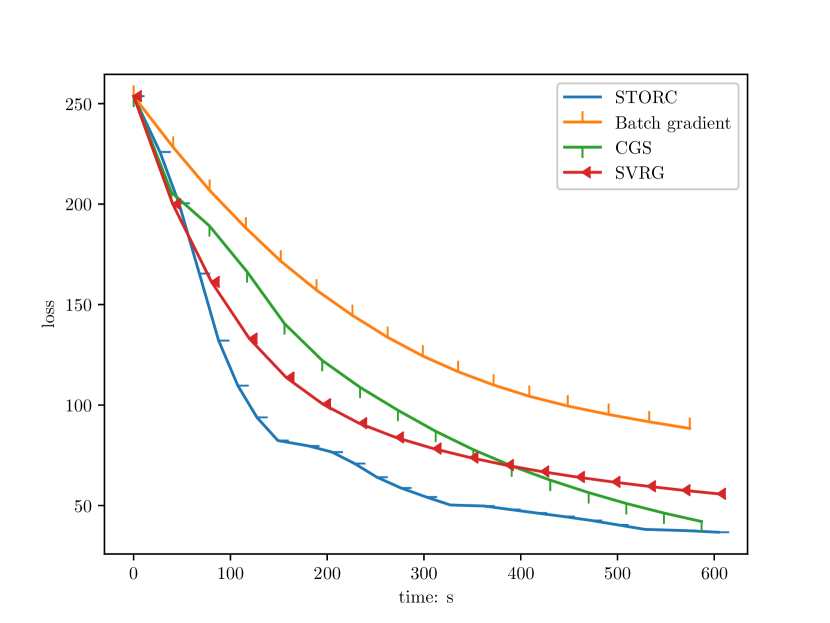
(a) $d=250,L/\hat{\sigma}=1000$

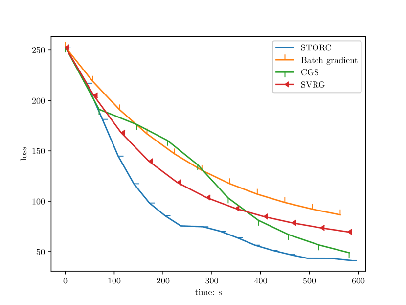
(b) $d=300,L/\hat{\sigma}=1000$

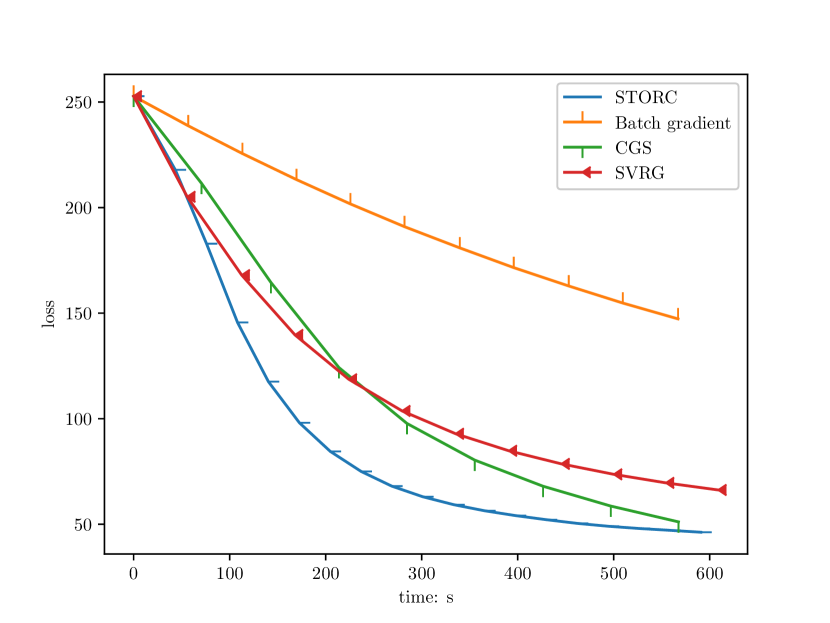
(c) $d=300,L/\hat{\sigma}=10000$

Figure 1: Plot of convex empirical loss $L_{n}(\Theta^{t})$ versus computation time.

We compare the performance of CGS and STORC with batch projected gradient descent and SVRG algorithm on matrix regression problem (9). For the convex loss problem we generate data $y_{i}=\langle X_{i},\Theta^{\star}\rangle+\epsilon_{i}$, here $\Theta^{\star}$ is a matrix with rank $r=5$ with $\left\lVert\Theta^{\star}\right\rVert_{*}=50$. We sample $\operatorname{vec}(X_{i})\sim N(0,\Sigma_{x})$ with $\Sigma_{x}$ being diagnal matrix in $\mathbb{R}^{d^{2}\times d^{2}}$ , and every diagnal entry is $\hat{\sigma}=1$ except the first one being $L$. We set $L=1000,10000$ to illustrate the impact of condition number performance. Finally we generate $n=\alpha rd$ samples with $\alpha=10$ and set $\rho=50$.

Figure 1 reports the simulation result for the convex loss problem. For batch algorithm CGS and projected gradient descent, the computation time per iteration is dominated by gradient evaluation. As our theorem has predicted, when the required precision is not too small, the CGS algorithm outperfoms projected gradient descent due to its acceleration in terms of gradient evaluation complexity (square root dependence on condition number). This is even more significant when we have ill-conditioned problem as in Figure 1(c). Both STORC and and SVRG outperform their batch counterparts by saving gradient evaluations significantly per iteration. Since STORC performs LO which only requires computing leading singular vectors, it outperforms SVRG which involves full SVD computation at each iteration. In fact we observe that SVRG could be even outperformed by CGS, which further emphasizes the importance of replacing full projection by linear optimization oracle.

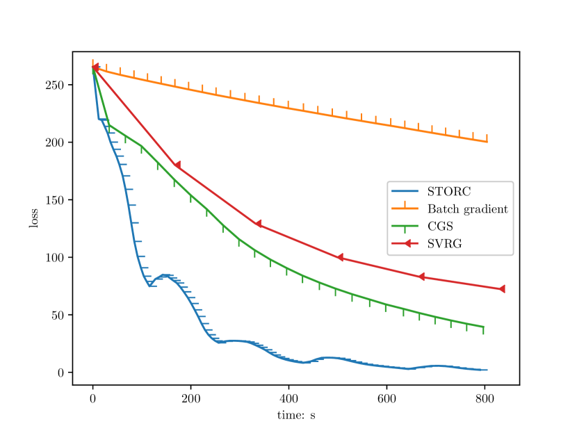
(a) $d=250,r=5$

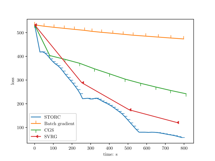
(b) $d=250,r=10$

(c) $d=300,r=5$

Figure 2: Plot of non-convex empirical loss $L_{n}(\Theta^{t})$ versus computation time.

For non-convex loss problem, we generate $y_{i}=\langle X_{i},\Theta^{\star}\rangle+\epsilon_{i}$ in the same way as the convex loss, where $\hat{\sigma}=1$ and $L=1000$. Instead of observing $X_{i}$ we only observe $Z_{i}=X_{i}+W_{i}$ where $\operatorname{vec}(W_{i})\sim N(0,0.1\cdot\hat{\sigma}I_{d^{2}})$ and independent of $X_{i}$. We generate sample of size $n=\alpha rd$ with $\alpha=10$ and set $\rho=50$. Figure 2 reports the simulation results for the non-convex loss. Again, CGS outperforms batch gradient descent by its accelerated performance in terms of gradient evaluation complexity. Notice that $\sigma_{max}(\Sigma_{w})\leqslant\sigma_{min}(\Sigma_{x})$ which by our theorem implies that non-convexity essentially causes no extra computational overhead for STORC algorithm. As predicted by our theoretical result, STORC outperforms SVRG by replacing projection step with the much cheaper linear oracle.

5 Conclusions

In this paper we show that batch and stochastic variants of Frank-Wolfe algorithm, namely CGS and STORC algorithm can be used to solve high dimensional statistical estimation problem efficiently, especially when the projection step in the gradient descent type algorithms is computationally hard. While the efficient gradient complexity result for CGS and STORC has been established in literature, such result requires the objective function $f(x)=\frac{1}{n}\sum_{i=1}^{n}f_{i}(x)$ being strongly convex and individual $f_{i}(x)$ being convex. In this paper we relax these restrictive assumptions that are hardly satisfied in high dimensional-statistics, by restricted strong convexity that holds true in various statistical mode and show that the same gradient evaluation complexity could be maintained under this more general condition.

 

Supplemental Material

Projection-Free Algorithms in Statistical Estimation

 

Appendix A Proof overview

In this section we provide a roadmap which we will following in establishing the complexity results presented in the paper.

It is convenient to note that an $L$-smooth function $f$ satisfies the following properties which is useful in our proof:

$$\displaystyle f(\lambda x+(1-\lambda)y)\geqslant\lambda f(x)+(1-\lambda)f(y)-\frac{L}{2}\lambda(1-\lambda)||x-y||^{2}$$ (26)

for $\lambda\in[0,1]$. If $f$ is additionally convex, then:

$$\left\lVert\nabla f(x)-\nabla f(y)\right\rVert^{2}\leqslant 2L\left(f(y)-f(x)-\langle\nabla f(x),y-x\rangle\right).$$ (27)

For simplicity of exposition, we emphasize the our proof scheme for convex case here. The basic idea of our proof is to re-analyze the convergence property of the aforementioned algorithms, while the strong convexity is replaced by the restricted strong convexity. More precisely, let $\hat{\Delta}_{t}=\theta_{t}-\hat{\theta}$, the first important lemma says that $\varphi(\hat{\Delta}_{t})$ in fact is close to $\left\lVert\hat{\Delta}_{t}\right\rVert$.

Lemma 2.

In problem (1), if $\varphi(\hat{\theta})=\rho$, then we have $\hat{\Delta}_{t}$ belongs to the set:

$$\mathbb{S}(\mathcal{M,\overline{M}})=\{\Delta:\,\varphi(\Delta)\leqslant 2\phi(\mathcal{\overline{M}})\left\lVert\Delta\right\rVert+2\varphi(\Pi_{\mathcal{M}}^{\perp}(\theta^{\star}))+2\varphi(\Delta^{\star})+2\phi(\overline{\mathcal{M}})\left\lVert\Delta^{\star}\right\rVert\}.$$ (28)

Now by combining (28) with the definition of restricted strong convexity, we have the following structure of pseudo strong convexity of the objective function that holds at the global optimum:

$$f(\theta)-f(\hat{\theta}) \geqslant\langle\nabla f(\hat{\theta}),\theta-\hat{\theta}\rangle+\frac{\sigma}{2}\left\lVert\theta-\hat{\theta}\right\rVert^{2}-\tau_{\sigma}\varphi(\theta-\hat{\theta})^{2}$$

$$\geqslant\frac{\hat{\sigma}}{2}\left\lVert\theta-\hat{\theta}\right\rVert^{2}-\hat{\sigma}\epsilon_{stat}^{2},$$ (29)

where the last inequality combines (28), Cauchy-Schwarz inequality and the definition of $\hat{\sigma},\epsilon_{stat}^{2}$.

To analyze the convergence of CGS and STORC, we first present a general convergence result of inner iteration. This theorem covers both the deterministic case as in CGS and the stochastic case as in STORC.

Theorem 3.

Fix outer iteration $t$, if we have for every inner iteration $i$ in CGS and STORC that $\mathbb{E}\left[\left\lVert\nabla_{i}-\nabla f(z_{i})\right\rVert^{2}\right]\leqslant\sigma_{i}^{2}$, then we have:

$$\mathbb{E}\left[f(y_{k})-f(\hat{\theta})\right]\leqslant\beta_{1}\Gamma_{k}\left\lVert x_{0}-\hat{\theta}\right\rVert^{2}+\Gamma_{k}\sum_{i=1}^{k}\left[\frac{\eta_{t,i}}{\Gamma_{i}}+\frac{\gamma_{i}\sigma_{i}^{2}}{2\Gamma_{i}(\beta_{i}-L\gamma_{i})}\right]$$ (30)

where we have defined $\Gamma_{i}$ as:

$$\Gamma_{i}=\begin{cases}1&i=1;\\ (1-\gamma_{i})\Gamma_{i-1}&i\geqslant 2.\end{cases}$$ (31)

Notice that for CGS algorithm which corresponds to the deterministic case, we have $\sigma_{i}=0$ for any iteration $i$. By specifying specific parameters in the two algorithms, we have concrete convergence results for inner iteration, provided we can control $\sigma_{i}^{2}$ to decrease in a certain rate. The proof of the following corollary is a simple induction after plugging in all the parameters into (30).

Corollary 3.

Fix outer iteration $t$, suppose we have $\mathbb{E}\left[\left\lVert x_{0}-\hat{\theta}\right\rVert^{2}\right]\leqslant D_{t}^{2}$, then by setting $\gamma_{k}=\frac{2}{k+1},\beta_{k}=\frac{3L}{k},\eta_{t,k}=\frac{2LD_{t}^{2}}{N_{t}k}$, if we can control $\sigma_{i}^{2}$ such that $\sigma_{i}^{2}\leqslant\frac{L^{2}D_{t}^{2}}{N_{t}(i+1)^{2}}$ for all $i\leqslant k$, then we have:

$$\mathbb{E}\left[f(y_{k})-f(\hat{\theta})\right]\leqslant\frac{8LD_{t}^{2}}{k(k+1)}.$$ (32)

Again, since $\sigma_{i}=0$ for CGS algorithm, the claim of corollary follows immediately once we have specified appropriate parameters. The main challenge of our proof, is to control $\sigma_{i}^{2}$ as prescribed by corollary for STORC algorithm.

We now explain why Corollary 3 almost completes our argument: if we can control $\sigma_{i}^{2}\leqslant\frac{L^{2}D_{t}^{2}}{N_{t}(i+1)^{2}}$ for all $i\leqslant N_{t}$, then by this corollary we have:

$$\mathbb{E}[f(\theta_{t})-f(\hat{\theta})] =\mathbb{E}[f(y_{N_{t}})-f(\hat{\theta})]$$

$$\leqslant\mathbb{E}[\frac{8L\left\lVert x_{0}-\hat{\theta}\right\rVert^{2}}{N_{t}(N_{t}+1)}]$$

$$\leqslant\mathbb{E}[\frac{16\hat{u}(f(\theta_{t-1})-f(\hat{\theta}))}{N_{t}(N_{t}+1)}],$$ (33)

where the first inequality uses $D_{t}=\left\lVert x_{0}-\hat{\theta}\right\rVert$, and in the second inequality we use the definition of condition number, the pseudo strong convexity (A) and the assumption that we have not achieved the statistical precision yet. Hence by specifying appropriate $N_{t}$ as in CGS and STORC, we establish the convergence for outer iteration is

$$\mathbb{E}[f(\theta_{t})-f(\hat{\theta})]\leqslant\frac{1}{2}\mathbb{E}[f(\theta_{t-1})-f(\hat{\theta})].$$ (34)

With this simple recursion for outer iteration and a careful summation of calls to gradient evaluation and linear optimization per iteration, the claim for CGS and STORC follows immediately, we leave the details of the proof in the rest of supplemental material.

Appendix B Proof of Lemma 1

Proof.

We have first

$$\mathcal{E}_{n}(\Delta) =L_{n}(\theta+\Delta)-L_{n}(\theta)-\langle\nabla L_{n}(\theta),\Delta\rangle$$

$$=\operatorname{vec}(\Delta)^{T}\hat{\Gamma}\operatorname{vec}(\Delta)$$ (35)

Define $\zeta(\Sigma)=\sup_{\left\lVert u\right\rVert_{2}=1,\left\lVert v\right\rVert_{2}=1}u^{T}\Sigma v$. For convex loss: We have $\mathcal{E}_{n}(\Delta)=\operatorname{vec}(\Delta)^{T}(\frac{1}{n}X^{T}X)\operatorname{vec}(\Delta)$, by Lemma 7 of Agarwal et al. (2010) we have there exists universl postive constants $c_{0},c_{1}$ such that:

$$\mathcal{E}_{n}(\Delta)\geqslant\frac{1}{2}\lambda_{min}(\Sigma_{x})\left\lVert\Delta\right\rVert_{F}^{2}-c_{1}\zeta(\Sigma_{x})\frac{d}{n}\left\lVert\Delta\right\rVert_{nuc}^{2}$$ (36)

with probability at least $1-\exp(-c_{0}n)$, which gives result for convex case.

For nonconvex loss, we have $\hat{\Gamma}=\frac{1}{n}Z^{T}Z-Z_{w}$, hence $\mathcal{E}_{n}(\Delta)=\operatorname{vec}(\Delta)^{T}(\frac{1}{n}Z^{T}Z)\operatorname{vec}(\Delta)-\operatorname{vec}(\Delta)^{T}\Sigma_{w}\operatorname{vec}(\Delta)=\mathcal{F}(\Delta)-\operatorname{vec}(\Delta)^{T}\Sigma_{w}\operatorname{vec}(\Delta)$. We have that with probability at least $1-\exp(-c_{0}n)$,

$$\mathcal{F}_{n}(\Delta)\geqslant\frac{1}{2}\lambda_{min}(\Sigma_{x})\left\lVert\Delta\right\rVert_{F}^{2}-c_{1}\zeta(\Sigma_{z})\frac{d}{n}\left\lVert\Delta\right\rVert_{nuc}^{2}$$ (37)

Now uses assumption that $\lambda_{max}(\Sigma_{w})\leqslant\frac{1}{4}\lambda_{min}(\Sigma_{x})$ we obtain result immediately. ∎

Appendix C Proof of Lemma 2

Proof.

First by notice that $\varphi(\hat{\theta})=\rho$, we have $\varphi(\theta_{t})\leqslant\varphi(\hat{\theta})$, then by triangle inequality we have

$$\varphi(\theta_{t})\leqslant\varphi(\theta^{\star})+\varphi(\Delta^{\star})\leqslant\varphi\left(\Pi_{\mathcal{M}}(\theta^{\star})\right)+\varphi\left(\Pi_{\mathcal{M}^{\perp}}(\theta^{\star})\right)+\varphi(\Delta^{\star})$$ (38)

Now we lower bound the left hand side using decomposibility of regularization, denote $\Delta_{t}=\theta_{t}-\theta^{\star}$:

$$\varphi(\theta_{t}) =\varphi\left(\Pi_{\mathcal{M}}(\theta^{\star})+\Pi_{\mathcal{M}^{\perp}}(\theta^{\star})+\Pi_{\mathcal{\overline{M}}}(\Delta_{t})+\Pi_{\mathcal{\overline{M}}^{\perp}}(\Delta_{t})\right)$$

$$\geqslant\varphi\left(\Pi_{\mathcal{M}}(\theta^{\star})+\Pi_{\mathcal{\overline{M}}^{\perp}}(\Delta_{t})\right)-\varphi\left(\Pi_{\mathcal{M}^{\perp}}(\theta^{\star})+\Pi_{\mathcal{\overline{M}}}(\Delta_{t})\right)$$

$$\geqslant\varphi\left(\Pi_{\mathcal{M}}(\theta^{\star})+\Pi_{\mathcal{\overline{M}}^{\perp}}(\Delta_{t})\right)-\varphi\left(\Pi_{\mathcal{M}^{\perp}}(\theta^{\star})\right)-\varphi\left(\Pi_{\mathcal{\overline{M}}}(\Delta_{t})\right)$$

$$=\varphi\left(\Pi_{\mathcal{M}}(\theta^{\star})\right)+\varphi\left(\Pi_{\mathcal{\overline{M}}^{\perp}}(\Delta_{t})\right)-\varphi\left(\Pi_{\mathcal{M}^{\perp}}(\theta^{\star})\right)-\varphi\left(\Pi_{\mathcal{\overline{M}}}(\Delta_{t})\right)$$ (39)

Now by combing (38) and (C) we have:

$$\varphi\left(\Pi_{\mathcal{\overline{M}}^{\perp}}(\Delta_{t})\right)\leqslant\varphi\left(\Pi_{\mathcal{\overline{M}}}(\Delta_{t})\right)+2\varphi\left(\Pi_{\mathcal{M}^{\perp}}(\theta^{\star})\right)+\varphi(\Delta^{\star})$$ (40)

which in turn by triangle inquality of $\varphi(\cdot)$ we have:

$$\varphi\left(\Delta_{t}\right)\leqslant 2\varphi\left(\Pi_{\mathcal{\overline{M}}}(\Delta_{t})\right)+2\varphi\left(\Pi_{\mathcal{M}^{\perp}}(\theta^{\star})\right)+\varphi(\Delta^{\star})$$ (41)

Finally we have:

$$\varphi\left(\hat{\Delta_{t}}\right) \leqslant\varphi\left(\Delta_{t}\right)+\varphi(\Delta^{\star})$$

$$\leqslant 2\varphi\left(\Pi_{\mathcal{\overline{M}}}(\Delta_{t})\right)+2\varphi\left(\Pi_{\mathcal{M}^{\perp}}(\theta^{\star})\right)+2\varphi(\Delta^{\star})$$

$$\leqslant 2\phi(\mathcal{\overline{M}})\left\lVert\Pi_{\mathcal{\overline{M}}}(\Delta_{t})\right\rVert+2\varphi\left(\Pi_{\mathcal{M}^{\perp}}(\theta^{\star})\right)+2\varphi(\Delta^{\star})$$

$$\leqslant 2\phi(\mathcal{\overline{M}})\left\lVert\Delta_{t}\right\rVert+2\varphi\left(\Pi_{\mathcal{M}^{\perp}}(\theta^{\star})\right)+2\varphi(\Delta^{\star})$$

$$\leqslant 2\phi(\mathcal{\overline{M}})\left\lVert\hat{\Delta_{t}}\right\rVert+2\phi(\mathcal{\overline{M}})\left\lVert\hat{\Delta^{\star}}\right\rVert+2\varphi\left(\Pi_{\mathcal{M}^{\perp}}(\theta^{\star})\right)+2\varphi(\Delta^{\star})$$ (42)

where the first inequality uses bound (41), the second equality uses definition of $\phi(\mathcal{\overline{M}})$, the third inequality uses non-expansiveness of projection and final inequality uses triangle inequality. ∎

Appendix D Proof of Theorem 3 and Corollary 3

D.1 Proof of Theorem 3

The proof of Theorem 3 is essentially centered around the analysis nesterov’s acceleration scheme, yet exact projection relaced by approximate projection with approximate precision controlled by wolfe gap. We present convergence result for stochastic case, which reduce to determinstic case (CGS) with $\sigma_{i}=0$.

Proof.

Let us fix outer iteration $t$. We first present an important inequality that characterize approximate solution:

$$\frac{1}{\beta_{k}}\langle\nabla_{k},x_{k}\rangle+\frac{1}{2}\left\lVert x_{k}-x\right\rVert^{2}\leqslant\frac{1}{\beta_{k}}\langle\nabla_{k},x\rangle+\frac{1}{2}\left\lVert x_{k-1}-x\right\rVert^{2}-\frac{1}{2}\left\lVert x_{k}-x_{k-1}\right\rVert^{2}+\frac{\eta_{t,k}}{\beta_{k}}$$ (43)

We note that (43) comes from wolfe gap condition that $x_{k}$ satisfies: $\langle\nabla_{k}+\beta_{k}(x_{k}-x_{k-1}),x_{k}-x\rangle\leqslant\eta_{t,k}$ with some algebraic manipulation. Now by convexity of $f$, definition of $z_{k},x_{k},y_{k}$ and smoothness we have:

$$f(y_{k}) \leqslant f(z_{k})+\langle\nabla f(z_{k}),y_{k}-z_{k}\rangle+\frac{L}{2}\left\lVert y_{k}-z_{k}\right\rVert^{2}$$

$$=(1-\gamma_{k})\left[f(z_{k})+\langle\nabla f(z_{k}),y_{k-1}-z_{k}\rangle\right]+\gamma_{k}\left[f(z_{k}+\langle\nabla f(z_{k}),x_{k}-z_{k}\rangle\right]+\frac{L\gamma_{k}^{2}}{2}\left\lVert x_{k}-x_{k-1}\right\rVert^{2}$$

$$\leqslant(1-\gamma_{k})f(y_{k-1})+\gamma_{k}\left[f(z_{k})+\langle\nabla f(z_{k}),x_{k}-z_{k}\rangle\right]+\frac{\beta_{k}\gamma_{k}}{2}\left\lVert x_{k}-x_{k-1}\right\rVert^{2}-\frac{\gamma_{k}}{2}(\beta_{k}-L\gamma_{k})\left\lVert x_{k}-x_{k-1}\right\rVert^{2}$$

Now let us denote $\delta_{k}=\nabla f(z_{k})-\nabla_{k}$, and apply projection inequality (43), we have:

$$f(y_{k}) \overset{(\ref{ub_3})}{\leqslant}(1-\gamma_{k})f(y_{k-1})+\gamma_{k}\left[f(z_{k})+\langle\nabla_{k},x_{k}-z_{k}\rangle\right]+\frac{\beta_{k}\gamma_{k}}{2}\left\lVert x_{k}-x_{k}\right\rVert^{2}$$

$$\qquad+\gamma_{k}\langle\delta_{k},x_{k}-z_{k}\rangle-\frac{\gamma_{k}}{2}(\beta_{k}-L\gamma_{k})\left\lVert x_{k}-x_{k-1}\right\rVert^{2}$$

$$\overset{(\ref{proj_lemma})}{\leqslant}(1-\gamma_{k})f(y_{k-1})+\gamma_{k}\left[f(z_{k})+\langle\nabla_{k},x-z_{k}\rangle\right]+\frac{\gamma_{k}\beta_{k}}{2}\left[\left\lVert x-x_{k-1}\right\rVert^{2}-\left\lVert x-x_{k}\right\rVert^{2}\right]$$

$$\qquad+\eta_{t,k}\gamma_{k}+\gamma_{k}\langle\delta_{k},x_{k}-z_{k}\rangle-\frac{\gamma_{k}}{2}(\beta_{k}-L\gamma_{k})\left\lVert x_{k}-x_{k-1}\right\rVert^{2}$$

$$=(1-\gamma_{k})f(y_{k-1})+\gamma_{k}\left[f(z_{k})+\langle\nabla f(z_{k}),x-z_{k}\rangle\right]+\frac{\gamma_{k}\beta_{k}}{2}\left[\left\lVert x-x_{k-1}\right\rVert^{2}-\left\lVert x-x_{k}\right\rVert^{2}\right]$$

$$\qquad+\eta_{t,k}\gamma_{k}+\gamma_{k}\langle\delta_{k},x_{k}-x\rangle-\frac{\gamma_{k}}{2}(\beta_{k}-L\gamma_{k})\left\lVert x_{k}-x_{k-1}\right\rVert^{2}$$ (45)

$$\leqslant(1-\gamma_{k})f(y_{k-1})+\gamma_{k}f(x)+\frac{\gamma_{k}\beta_{k}}{2}\left[\left\lVert x-x_{k-1}\right\rVert^{2}-\left\lVert x-x_{k}\right\rVert^{2}\right]$$

$$\qquad+\eta_{t,k}\gamma_{k}+\gamma_{k}\langle\delta_{k},x_{k-1}-x\rangle+\gamma_{k}\langle\delta_{k},x_{k}-x_{k-1}\rangle-\frac{\gamma_{k}}{2}(\beta_{k}-L\gamma_{k})\left\lVert x_{k}-x_{k-1}\right\rVert^{2}$$

$$\leqslant(1-\gamma_{k})f(y_{k-1})+\gamma_{k}f(x)+\frac{\gamma_{k}\beta_{k}}{2}\left[\left\lVert x-x_{k-1}\right\rVert^{2}-\left\lVert x-x_{k}\right\rVert^{2}\right]$$

$$\qquad+\eta_{t,k}\gamma_{k}+\gamma_{k}\langle\delta_{k},x_{k-1}-x\rangle+\gamma_{k}\left\lVert\delta_{k}\right\rVert\left\lVert x_{k}-x_{k-1}\right\rVert-\frac{\gamma_{k}}{2}(\beta_{k}-L\gamma_{k})\left\lVert x_{k}-x_{k-1}\right\rVert^{2}$$

By applying basic inequality $bt-\frac{at^{2}}{2}\leqslant\frac{b^{2}}{2a}$ to the last line of previous inequality we have:

$$f(y_{k}) \leqslant(1-\gamma_{k})f(y_{k-1})+\gamma_{k}f(x)+\frac{\gamma_{k}\beta_{k}}{2}\left[\left\lVert x-x_{k-1}\right\rVert^{2}-\left\lVert x-x_{k}\right\rVert^{2}\right]$$

$$\qquad+\eta_{t,k}\gamma_{k}+\gamma_{k}\langle\delta_{k},x_{k-1}-x\rangle+\frac{\left\lVert\delta_{k}\right\rVert^{2}\gamma_{k}}{\beta_{k}-L\gamma_{k}}$$ (46)

Now take expectation of both sizes with obsevation that $\mathbb{E}[\langle\delta_{k},x_{k-1}-x\rangle]=0$ and $\mathbb{E}[\left\lVert\delta_{k}\right\rVert^{2}]=\sigma_{k}^{2}$, we have:

$$\mathbb{E}[f(y_{k})-f(x)] \leqslant(1-\gamma_{k})\mathbb{E}[f(y_{k-1})-f(x)]+\frac{\gamma_{k}\beta_{k}}{2}\mathbb{E}\left[\left\lVert x-x_{k-1}\right\rVert^{2}-\left\lVert x-x_{k}\right\rVert^{2}\right]$$

$$\qquad+\eta_{t,k}\gamma_{k}+\frac{\sigma_{k}^{2}\gamma_{k}}{\beta_{k}-L\gamma_{k}}$$ (47)

Devide both sides by $\Gamma_{k}$ and by definition of $\Gamma_{k}$ we have:

$$\frac{1}{\Gamma_{k}}\mathbb{E}[f(y_{k})-f(x)] \leqslant\frac{1}{\Gamma_{k-1}}\mathbb{E}[f(y_{k-1})-f(x)]+\frac{\gamma_{k}\beta_{k}}{2\Gamma_{k}}\mathbb{E}\left[\left\lVert x-x_{k-1}\right\rVert^{2}-\left\lVert x-x_{k}\right\rVert^{2}\right]$$

$$\qquad+\frac{\eta_{t,k}\gamma_{k}}{\Gamma_{k}}+\frac{\sigma_{k}^{2}\gamma_{k}}{\Gamma_{k}(\beta_{k}-L\gamma_{k})}$$ (48)

Now sum up (D.1) from $i=1$ to $k$ we have:

$$\mathbb{E}[f(y_{k})-f(x)] \leqslant\Gamma_{k}(1-\gamma_{1})\mathbb{E}[f(y_{0})-f(x)]+\Gamma_{k}\sum_{i=1}^{k}\frac{\gamma_{i}\beta_{i}}{2\Gamma_{i}}\mathbb{E}\left[\left\lVert x-x_{i-1}\right\rVert^{2}-\left\lVert x-x_{i}\right\rVert^{2}\right]$$

$$\qquad+\Gamma_{k}\sum_{i=1}^{k}\frac{\eta_{t,i}\gamma_{i}}{\Gamma_{i}}+\Gamma_{k}\sum_{i=1}^{k}\frac{\sigma_{i}^{2}\gamma_{i}}{\Gamma_{i}(\beta_{i}-L\gamma_{i})}$$

$$=\Gamma_{k}(1-\gamma_{1})\mathbb{E}[f(y_{0})-f(x)]$$

$$\qquad+\Gamma_{k}\left(\frac{\gamma_{1}\beta_{1}}{\Gamma_{1}}\mathbb{E}\left\lVert x-x_{0}\right\rVert^{2}+\sum_{i=2}^{k}(\frac{\gamma_{i}\beta_{i}}{2\Gamma_{i}}-\frac{\gamma_{i-1}\beta_{i-1}}{2\Gamma_{i-1}})\mathbb{E}\left\lVert x-x_{i}\right\rVert^{2}-\frac{\gamma_{k}\beta_{k}}{2\Gamma_{k}}\mathbb{E}\left\lVert x-x_{k}\right\rVert^{2}\right)$$

$$\qquad+\Gamma_{k}\sum_{i=1}^{k}\frac{\eta_{t,i}\gamma_{i}}{\Gamma_{i}}+\Gamma_{k}\sum_{i=1}^{k}\frac{\sigma_{i}^{2}\gamma_{i}}{\Gamma_{i}(\beta_{i}-L\gamma_{i})}$$

$$\leqslant\Gamma_{k}\beta_{1}\mathbb{E}\left\lVert x-x_{0}\right\rVert^{2}+\Gamma_{k}\sum_{i=1}^{k}\frac{\eta_{t,i}\gamma_{i}}{\Gamma_{i}}+\Gamma_{k}\sum_{i=1}^{k}\frac{\sigma_{i}^{2}\gamma_{i}}{\Gamma_{i}(\beta_{i}-L\gamma_{i})}$$ (49)

where (D.1) uses our parameter choice such that $\frac{\gamma_{i}\beta_{i}}{\Gamma_{i}}\leqslant\frac{\gamma_{i-1}\beta_{i-1}}{\Gamma_{i-1}}$ and definition $\gamma_{1}=1$. ∎

D.2 Proof of Corollary 3

The proof of this corollary is simply plug in our parameter choice in the statement, and do a simple induction, we omit the details here.

Appendix E Proof of Corollary 1 and Corollary 2

E.1 Proof of Corollary 1

Proof.

By Lemma 1 we have that $\tau_{\sigma}=\frac{\xi(\Sigma_{x})d}{n}$, next we choose appropriate subspace pair $(\mathcal{M},\overline{\mathcal{M}}^{\perp})$ to control the tradeoff between denominator and nominator in the definition of $\epsilon_{stat}^{2}=\tau_{\sigma}(\varphi(\Pi_{\mathcal{M}^{\perp}}(\theta^{\star}))+2\varphi(\Delta^{\star})+\phi(\overline{\mathcal{M}})\left\lVert\Delta^{\star}\right\rVert)^{2}/\hat{\sigma}$.

Let $\Theta^{\star}=UDV^{T}$ be singular value decomposition of ground truth with rank $r$, let $U^{r}$ and $V^{r}$ be first $r$ columns of $U$ and $V$, define:

$$\mathcal{M} =\{\Theta\in\mathbb{R}^{d\times d}:col(\Theta)\subseteq col(U^{r}),\,col(\Theta^{T})\subseteq col(V^{r})\}$$

$$\mathcal{\overline{M}^{\perp}} =\{\Theta\in\mathbb{R}^{d\times d}:col(\Theta)\subseteq col(U^{r})^{\perp},\,col(\Theta^{T})\subseteq col(V^{r})^{\perp}\}$$

notice now that $\Theta^{\star}\in\mathcal{M}$ and by definition we have $\phi^{2}(\overline{M})\leqslant r$, hence we have:

$$\left(\varphi(\Pi_{\mathcal{M^{\perp}}}(\Theta^{\star})+2\varphi(\Delta^{\star})+\phi(\overline{\mathcal{M}})\left\lVert\Delta^{\star}\right\rVert\right)^{2}\leqslant 12\varphi^{2}(\Delta^{\star})+3r\left\lVert\Delta^{\star}\right\rVert^{2}=12\left\lVert\Delta^{\star}\right\rVert_{nuc}^{2}+3r\left\lVert\Delta^{\star}\right\rVert_{F}^{2}$$ (50)

We use an inequality which will be verified later: $\left\lVert\Delta^{\star}\right\rVert_{nuc}^{2}\leqslant 4r\left\lVert\Delta^{\star}\right\rVert_{F}^{2}$, summarizing all above we have:

$$\epsilon_{stat}^{2}=\frac{\xi(\Sigma_{x})d}{n\hat{\sigma}}\cdot cr\left\lVert\Delta^{\star}\right\rVert_{F}^{2}$$ (51)

for some constant $c$.

Now $L=\sigma_{max}(\Sigma_{x})$, $\hat{\sigma}=\sigma_{min}(\Sigma_{x})-\frac{\xi(\Sigma_{x})rd}{n}$ follows directy from its definition and Lemma 1, with scaling $n=\Omega(\frac{\xi(\Sigma_{x})r}{d\sigma_{min}(\Sigma_{x})})$ we have $\hat{\sigma}=c_{1}\sigma_{min}(\Sigma_{x})$ for some constant $c_{1}$. And we also have simple inequality $\left\lVert X\right\rVert_{F}^{2}\leqslant\left\lVert X\right\rVert_{nuc}^{2}$ for any matrix, hence $D\leqslant\rho$, plug in specification of $L,\hat{\sigma},D$ yields bound on gradient evaluation and linear oracle. Finally the scaling of $n=\Omega(\frac{\xi(\Sigma_{x})rd}{\sigma_{\min}(\Sigma_{x})})$ would also gives us $\epsilon_{stat}^{2}\leqslant c_{2}\left\lVert\Delta^{\star}\right\rVert_{F}^{2}$, which gives us the bound on distance to optimum.

It remains to show $\left\lVert\Delta^{\star}\right\rVert_{nuc}^{2}\leqslant 4r\left\lVert\Delta^{\star}\right\rVert_{F}^{2}$, this is very similar to the proof of Lemma 2, using condition that $\varphi(\hat{\theta})\leqslant\rho\leqslant$ and use triangle inequality we have $\varphi(\hat{\theta})\leqslant\varphi(\Pi_{\mathcal{M}}(\theta^{\star}))+\varphi(\Pi_{\mathcal{M}^{\perp}}(\theta^{\star}))$. Now we lower bound the left hand side.

$$\varphi(\hat{\theta}) =\varphi(\theta^{\star}+\delta^{\star})$$

$$=\varphi(\Pi_{\mathcal{M}}(\theta^{\star})+\Pi_{\mathcal{M}^{\perp}}(\theta^{\star})+\Pi_{\mathcal{\overline{M}}}(\Delta^{\star})+\Pi_{\mathcal{\overline{M^{\perp}}}}(\Delta^{\star}))$$

$$\geqslant\varphi(\Pi_{\mathcal{M}}(\theta^{\star})+\Pi_{\mathcal{\overline{M^{\perp}}}}(\Delta^{\star}))-\varphi(\Pi_{\mathcal{M}^{\perp}}(\theta^{\star}))-\varphi(\Pi_{\mathcal{\overline{M}}}(\Delta^{\star}))$$

$$=\varphi(\Pi_{\mathcal{M}}(\theta^{\star}))+\varphi(\Pi_{\mathcal{\overline{M^{\perp}}}}(\Delta^{\star}))-\varphi(\Pi_{\mathcal{M}^{\perp}}(\theta^{\star}))-\varphi(\Pi_{\mathcal{\overline{M}}}(\Delta^{\star}))$$

combined with the upper bound we have:

$$\varphi(\Pi_{\mathcal{\overline{M^{\perp}}}}(\Delta^{\star}))\leqslant\varphi(\Pi_{\mathcal{\overline{M}}}(\Delta^{\star}))+2\varphi(\Pi_{\mathcal{M}^{\perp}}(\theta^{\star}))$$

which by triangle inequality implies:

$$\varphi(\Delta^{\star}) \leqslant 2\varphi(\Pi_{\mathcal{\overline{M}}}(\Delta^{\star}))+2\varphi(\Pi_{\mathcal{M}^{\perp}}(\theta^{\star}))$$

$$\leqslant 2\phi(\overline{\mathcal{M}})\left\lVert\Pi_{\mathcal{\overline{M}}}(\Delta^{\star})\right\rVert+2\varphi(\Pi_{\mathcal{M}^{\perp}}(\theta^{\star}))$$

$$\leqslant 2\phi(\overline{\mathcal{M}})\left\lVert\Delta^{\star}\right\rVert+2\varphi(\Pi_{\mathcal{M}^{\perp}}(\theta^{\star}))$$

notice now that by out definition of $\mathcal{M}$ in the example we have $\varphi(\Pi_{\mathcal{M}^{\perp}}(\theta^{\star}))=0$, specifically we have: $\left\lVert\Delta^{\star}\right\rVert_{nuc}\leqslant 2\phi(\overline{\mathcal{M}})\left\lVert\Delta^{\star}\right\rVert_{F}$, now take square on both sides and use the fact that $\phi^{2}(\overline{\mathcal{M}})=r$ gives $\left\lVert\Delta^{\star}\right\rVert_{nuc}^{2}\leqslant 4r\left\lVert\Delta^{\star}\right\rVert_{F}^{2}$. ∎

E.2 Proof of Corollary 2

Proof.

This is essentially the same as in proof of corollary 1,under the scaling $n=\Omega(\frac{\xi(\Sigma_{x})dr}{\sigma_{min}(\Sigma_{x})})$ we have modular some costants, $\epsilon_{stat}^{2}=\frac{\xi(\Sigma_{x})dr}{n\hat{\sigma}}\left\lVert\Delta^{\star}\right\rVert_{F}^{2},L=\sigma_{max}(\Sigma_{x}),\hat{\sigma}=\sigma_{\min}(\Sigma_{x}),D=\rho$ plug in these into theorem 2 yields the result. ∎

Appendix F Proof of Theorem 1 and Theorem 2: Convex Case

We are now ready to prove our main theorem, as stated before if condition of Corollary 3 holds for both CGS and STORC, then we can do this in a unified way. As we will show in the proof, the parameter specification of $\beta_{k},\gamma_{k},\eta_{t,k}$ in both CGS and STORC will satisfy condition in the corollary for some $D_{t}$, the remaining work is to control $\sigma_{i}^{2}$. Since CGS algorithm is determinstic, we now only need to control $\sigma_{i}^{2}$ in STORC algorithm, and this is where variance reduction came into play.

Proof.

We will show by induction that

$$\mathbb{E}\left[f(\theta_{t})-f(\hat{\theta})\right]\leqslant\frac{\delta_{0}}{2^{t}}$$ (52)

For base case $t=0$, $\mathbb{E}\left[f(\theta_{0})-f(\hat{\theta})\right]\leqslant\delta_{0}$ by definition.

Analysis for STORC: Suppose the (52) holds for all outer iteration before iteration $t$, we now focus on interation $t$. First we upper bound the variance of $\nabla_{k}$ in STORC algorithm. We claim that:

$$\mathbb{E}[\left\lVert\nabla f_{j}(z_{k})-\nabla f_{j}(y_{0})+\nabla f(y_{0})-\nabla f(z_{k})\right\rVert^{2}]\leqslant 4L\mathbb{E}\left([f(z_{k})-f(\hat{\theta})]+[f(y_{0})-f(\hat{\theta})]\right)$$ (53)

We note that by construction of $\nabla_{k}$ we have:

$$\sigma_{i}^{2} =\frac{1}{m_{t,i}}\mathbb{E}\left\lVert\nabla f_{j}(z_{i})-\nabla f_{j}(y_{0})+\nabla f(y_{0})-\nabla f(z_{i})\right\rVert^{2}$$

$$\leqslant\frac{4L}{m_{t,i}}\mathbb{E}\left([f(z_{i})-f(\hat{\theta})]+[f(y_{0})-f(\hat{\theta})]\right)$$ (54)

For now we assume (53) holds, and we next show $\sigma_{i}^{2}\leqslant\frac{L^{2}D_{t}^{2}}{N_{t}(i+1)^{2}}$ by induction.

For base case $i=1$, notice that $z_{0}=y_{0}=x_{0}$, by (F) we have:

$$\sigma_{1}^{2}\leqslant\frac{8L}{m_{t,1}}\mathbb{E}[f(y_{0})-f(\hat{\theta})] =\frac{8L}{m_{t,1}}\mathbb{E}[f(\theta_{t-1})-f(\hat{\theta})]\leqslant\frac{8L\delta_{0}}{m_{t,1}2^{t-1}}$$ (55)

Now by pseudo strong convexity (A) and assumption that we have not converged to statistical precision, we have:

$$\mathbb{E}\left\lVert x_{0}-\hat{\theta}\right\rVert^{2} \leqslant\mathbb{E}\left[\frac{(f(x_{0})-f(\hat{\theta}))+\hat{\sigma}\epsilon_{stat}^{2}}{\hat{\sigma}}\right]$$

$$\leqslant\mathbb{E}\left[\frac{2(f(x_{0})-f(\hat{\theta}))}{\hat{\sigma}}\right]$$

$$\leqslant\frac{\delta_{0}}{2^{t-2}\hat{\sigma}}$$ (56)

Hence we can choose $D_{t}^{2}=\frac{\delta_{0}}{2^{t-2}\hat{\sigma}}$, combine this with (55) we have $\sigma_{1}^{2}\leqslant\frac{4LD_{t}^{2}\hat{\sigma}}{m_{t,1}}\leqslant\frac{L^{2}D_{t}^{2}}{4N_{t}}$, the proof for $i=1$ completes.

Suppose (53) holds for $i<k$, by (F) to control $\sigma_{k}^{2}$ we need to upper bound $f(z_{k})$. Now by definition of $z_{k},x_{k},y_{k}$ and $\gamma_{k}$ we have:

$$y_{k-1}=\frac{k+1}{2k-1}z_{k}+\frac{k-2}{2k-1}y_{k-2}$$ (57)

Together with smoothness property (26) we have:

$$f(y_{k-1})-f(\hat{\theta}) \geqslant\frac{k+1}{2k-1}\left(f(z_{k})-f(\hat{\theta})\right)+\frac{k-2}{2k-1}\left(f(y_{k-2})-f(\hat{\theta})\right)-\frac{L(s+1)(s-2)}{2(2s-1)^{2}}\left\lVert z_{k}-y_{k-2}\right\rVert^{2}$$

$$\geqslant\frac{1}{2}\left(f(z_{k})-f(\hat{\theta})\right)-\frac{L}{2}\left\lVert y_{k-1}-y_{k-2}\right\rVert^{2}$$

Rearrange terms, use cauchy-schwarz inequality and pseudo strong convexity (A) we have upper bound for $f(z_{k})$:

$$\mathbb{E}\left[f(z_{k})-f(\hat{\theta})\right] \leqslant 2\mathbb{E}\left(f(y_{k-1})-f(\hat{\theta})\right)+L\mathbb{E}\left\lVert y_{k-1}-y_{k-2}\right\rVert^{2}$$

$$\leqslant 2\mathbb{E}\left(f(y_{k-1})-f(\hat{\theta})\right)+2L\mathbb{E}(\left\lVert y_{k-1}-\hat{\theta}\right\rVert^{2}+\left\lVert y_{k-2}-\hat{\theta}\right\rVert^{2})$$

$$\overset{(\ref{pseudo-sc})}{\leqslant}2\mathbb{E}\left(f(y_{k-1})-f(\hat{\theta})\right)+2L\mathbb{E}\left(\frac{f(y_{k-1})-f(\hat{\theta})+\hat{\sigma}\epsilon_{stat}^{2}}{\hat{\sigma}}+\frac{f(y_{k-2})-f(\hat{\theta})+\hat{\sigma}\epsilon_{stat}^{2}}{\hat{\sigma}}\right)$$

$$\leqslant 2\mathbb{E}\left(f(y_{k-1})-f(\hat{\theta})\right)+\frac{8L}{\hat{\sigma}}\mathbb{E}\left([f(y_{k-1})-f(\hat{\theta})]+[f(y_{k-2})-f(\hat{\theta})]\right)$$ (59)

$$\leqslant\frac{2L}{\hat{\sigma}}\mathbb{E}\left(f(y_{k-1})-f(\hat{\theta})\right)+\frac{8L}{\hat{\sigma}}\mathbb{E}\left([f(y_{k-1})-f(\hat{\theta})]+[f(y_{k-2})-f(\hat{\theta})]\right)$$ (60)

Note that in (59) we uses our assumption that we have not converged to statistical precision yet, that is $\text{min}\{\mathbb{E}[f(y_{k-1})-f(\hat{\theta})],\mathbb{E}[f(y_{k-2})-f(\hat{\theta})]\}\geq\hat{\sigma}\epsilon_{stat}^{2}$.

Now using (60) we can utilize upper bound for $f(y_{k-1})$ and $f(y_{k-2})$. Using induction hypothesis that (53) holds for $i<k$, by an application of Corollary 3 we know that $\mathbb{E}[f(y_{k-1})-f(\hat{\theta})]\leqslant\frac{8LD_{t}^{2}}{k(k-1)}$ and $\mathbb{E}[f(y_{k-2})-f(\hat{\theta})]\leqslant\frac{8LD_{t}^{2}}{(k-2)(k-1)}$, note $\hat{u}=\frac{L}{\hat{\sigma}}$, we have:

$$\mathbb{E}[f(z_{k})-f(\hat{\theta})] \leqslant 10\hat{u}\mathbb{E}\left(f(y_{k-1})-f(\hat{\theta})\right)+8\hat{u}\mathbb{E}\left(f(y_{k-2})-f(\hat{\theta})\right)$$

$$\leqslant\frac{80\hat{u}LD_{t}^{2}}{k(k-1)}+\frac{64\hat{u}LD_{t}^{2}}{(k-2)(k-1)}$$

$$\leqslant\frac{1200\hat{u}LD_{t}^{2}}{(k+1)^{2}}$$ (61)

Finally, by plugging the above result in (F) we have:

$$\sigma_{k}^{2} \leqslant\frac{4L}{m_{t,k}}\mathbb{E}\left([f(z_{k})-f(\hat{\theta})]+[f(y_{0})-f(\hat{\theta})]\right)$$

$$\leqslant\frac{4L}{m_{t,k}}\left(\frac{1200\hat{u}LD_{t}^{2}}{(k+1)^{2}}+\frac{\delta_{0}}{2^{t-1}}\right)$$

$$=\frac{4L}{m_{t,k}}\left(\frac{1200\hat{u}LD_{t}^{2}}{(k+1)^{2}}+\frac{2LD_{t}^{2}}{\hat{u}}\right)$$

$$\leqslant\frac{4L}{m_{t,k}}\left(\frac{1200\hat{u}LD_{t}^{2}}{(k+1)^{2}}+\frac{64LD_{t}^{2}}{(N_{t}+1)^{2}}\right)$$

$$\leqslant\frac{4L}{m_{t,k}}\left(\frac{1200\hat{u}LD_{t}^{2}}{(k+1)^{2}}+\frac{64LD_{t}^{2}}{(k+1)^{2}}\right)$$

$$\leqslant\frac{L^{2}D_{t}^{2}}{N_{t}(k+1)^{2}}$$ (62)

where the last inequality uses our choice of $m_{t,k}$. We have now completed inductinon for showing $\sigma_{k}^{2}\leqslant\frac{L^{2}D_{t}^{2}}{N_{t}(k+1)^{2}}$ for $k=1\text{ to }N_{t}$, by choosing $k=N_{t}$ and use corollary (3) we have:

$$\mathbb{E}[f(y_{N_{t}})-f(\hat{\theta})] \leqslant\frac{8LD_{t}^{2}}{N_{t}(N_{t}+1)}$$

$$\leqslant\frac{\delta_{0}}{2^{t}}$$ (63)

where the last inequality comes from our choice of $N_{t}$. By $f(\theta_{t})=f(y_{N_{t}})$ we have also completed induction for outer iteration.

Analysis for CGS: Since $\sigma_{k}^{2}=0$ for $k=1\text{ to }N_{t}$, choose $D_{t}^{2}$ as in STORC algorithm, by corollary 3 we immeditely have that $f(\theta_{t})-f(\hat{\theta})\leqslant\frac{8LD_{t}^{2}}{N_{t}(N_{t}+1)}\leqslant\frac{\delta_{0}}{2^{t}}$ by our choice of $N_{t}$.

Parameter Specification: We should note that both CGS and STORC uses exactly the same paramter specification for $\gamma_{k}=\frac{2}{k+1},\beta_{k}=\frac{3L}{k}$, and $\eta_{t,k}=\frac{8L\delta_{0}}{\hat{\sigma}2^{t}N_{t}k}=\frac{2LD_{t}^{2}}{N_{t}k}$, hence they all meet the condition in corollary 3.

Gradient Complexity and LO Complexity: Now we need to sum up calls to gradient evaluation complexity, by (52) we know that to get $\epsilon$-precision solution we need $T=\log_{2}(\frac{\delta_{0}}{\epsilon})$ outer iteration for both CGS and STORC.

For CGS algorithm calls to gradient evalution is bounded by:

$$\sum_{t=1}^{T}N_{t}=\mathcal{O}(T\sqrt{\hat{u}})=\mathcal{O}\left(\sqrt{\frac{L}{\hat{\sigma}}}\log(\frac{\delta_{0}}{\epsilon})\right)$$ (64)

it was shown that duality gap of frank-wolfe algorithm decrease with rate $\mathcal{O}(\frac{1}{m})$, and to solve projection approximately in the algorithm takes $\mathcal{O}\left(\frac{\beta_{k}D^{2}}{\eta_{t,k}}\right)$ iteration Jaggi (2013), hence we have calls to the linear oracle bounded by:

$$\sum_{t=1}^{T}\sum_{k=1}^{N_{t}}\mathcal{O}\left(\frac{\beta_{k}D^{2}}{\eta_{t,k}}+1\right) =\sum_{t=1}^{T}\mathcal{O}\left(\frac{N_{t}^{2}D^{2}}{D_{t}^{2}}+N_{t}\right)$$

$$=\sum_{t=1}^{T}\mathcal{O}\left(\frac{2^{t}LD^{2}}{\delta_{0}}+N_{t}\right)$$

$$=\mathcal{O}\left(\frac{LD^{2}}{\epsilon}+\sqrt{\frac{L}{\hat{\sigma}}}\log(\frac{\delta_{0}}{\epsilon})\right)$$ (65)

For STORC algorithm calls to stochastic gradient evaluation is bounded by:

$$\sum_{t=1}^{T}(n+\sum_{k=1}^{N_{t}}m_{t,k}) =\sum_{t=1}^{T}\mathcal{O}\left(n+N_{t}^{2}\hat{u}\right)$$

$$=\mathcal{O}\left((n+(\frac{L}{\hat{\sigma}})^{2})\log_{2}(\frac{\delta_{0}}{\epsilon})\right)$$ (66)

and similar to CGS, the calls to the linear oracle is bounded by:

$$\sum_{t=1}^{T}\sum_{k=1}^{N_{t}}\mathcal{O}\left(\frac{\beta_{k}D^{2}}{\eta_{t,k}}+1\right) =\sum_{t=1}^{T}\mathcal{O}\left(\frac{N_{t}^{2}D^{2}}{D_{t}^{2}}+N_{t}\right)$$

$$=\sum_{t=1}^{T}\mathcal{O}\left(\frac{2^{t}LD^{2}}{\delta_{0}}+N_{t}\right)$$

$$=\mathcal{O}\left(\frac{LD^{2}}{\epsilon}+\sqrt{\frac{L}{\hat{\sigma}}}\log(\frac{\delta_{0}}{\epsilon})\right)$$ (67)

∎

The only remaining part is to show the upper bound for variance of stochastic gradient (53):

Proof.

$$\mathbb{E}[\left\lVert\nabla f_{j}(z_{k})-\nabla f_{j}(y_{0})+\nabla f(y_{0})-\nabla f(z_{k})\right\rVert^{2}]$$

$$\leqslant\mathbb{E}[\left\lVert\nabla f_{j}(z_{k})-\nabla f_{j}(y_{0}))\right\rVert^{2}]$$

$$=\mathbb{E}[\left\lVert(\nabla f_{j}(z_{k})-\nabla f_{j}(\hat{\theta}))-(\nabla f_{j}(y_{0})-\nabla f_{j}(\hat{\theta}))\right\rVert^{2}]$$

$$\leqslant 2\mathbb{E}\left(\left\lVert\nabla f_{j}(z_{k})-\nabla f_{j}(\hat{\theta})\right\rVert^{2}+\left\lVert\nabla f_{j}(y_{0})-\nabla f_{j}(\hat{\theta})\right\rVert^{2}\right)$$

$$\overset{(\ref{convex-smooth})}{\leqslant}4L\mathbb{E}\left([f_{j}(z_{k})-f_{j}(\hat{\theta})-\langle\nabla f_{j}(\hat{\theta}),z_{k}-\hat{\theta}\rangle]+[f_{j}(y_{0})-f_{j}(\hat{\theta})-\langle\nabla f_{j}(\hat{\theta}),y_{0}-\hat{\theta}\rangle]\right)$$

$$=4L\mathbb{E}\left([f(z_{k})-f(\hat{\theta})-\langle\nabla f(\hat{\theta}),z_{k}-\hat{\theta}\rangle]+f(y_{0})-f(\hat{\theta})-\langle\nabla f(\hat{\theta}),y_{0}-\hat{\theta}\rangle]\right)$$

$$\leqslant 4L\mathbb{E}\left([f(z_{k})-f(\hat{\theta})]+[f(y_{0})-f(\hat{\theta})]\right)$$ (68)

where the last inequality uses optimality of $\hat{\theta}$. ∎

Appendix G Proof of Theorem 1 and Theorem 2: Non-convex Case

G.1 Proof of Theorem 1

Proof.

By definition of restricted strong convexity we have:

$$f(\hat{\theta})-f(\theta)\leqslant\langle\nabla f(\theta),\hat{\theta}-\theta\rangle+\frac{\hat{\sigma}}{2}\left\lVert\theta-\hat{\theta}\right\rVert^{2}-\hat{\sigma}\epsilon_{stat}^{2}$$ (69)

Now pluging this bound into (45) with $\theta=z_{k}$ and $x=\hat{\theta}$ we obtain:

$$f(y_{k}) \leqslant(1-\gamma_{k})f(y_{k-1})+\gamma_{k}f(\hat{\theta})+\gamma_{k}\hat{\sigma}\epsilon_{stat}^{2}+\frac{\gamma_{k}\beta_{k}}{2}\left[\left\lVert\hat{\theta}-x_{k-1}\right\rVert^{2}-\left\lVert\hat{\theta}-x_{k}\right\rVert^{2}\right]$$

$$\qquad+\eta_{t,k}\gamma_{k}+\gamma_{k}\langle\delta_{k},x_{k-1}-\hat{\theta}\rangle+\gamma_{k}\langle\delta_{k},x_{k}-x_{k-1}\rangle-\frac{\gamma_{k}}{2}(\beta_{k}-L\gamma_{k})\left\lVert x_{k}-x_{k-1}\right\rVert^{2}$$

Following exactly the same argument in the proof of Theorem 3, we would end up having:

$$f(y_{k})-f(\hat{\theta}) \leqslant\Gamma_{k}\beta_{1}\mathbb{E}\left\lVert\hat{\theta}-x_{0}\right\rVert^{2}+\Gamma_{k}\sum_{i=1}^{k}\frac{\eta_{t,i}\gamma_{i}}{\Gamma_{i}}+\Gamma_{k}\sum_{i=1}^{k}\frac{\gamma_{i}\hat{\sigma}\epsilon_{stat}^{2}}{\Gamma_{i}}$$ (70)

We again will proceed with induction by showing that $f(\theta_{t})-f(\hat{\theta})\leqslant\frac{\delta_{0}}{2^{t}}$. The base case is trivial by definition of $\delta_{0}$. Now suppose the claim holds before iteration $t$, then by pseudo strong convexity (A) we have:

$$\mathbb{E}\left\lVert x_{0}-\hat{\theta}\right\rVert^{2} \leqslant\mathbb{E}\left[\frac{(f(x_{0})-f(\hat{\theta}))+\hat{\sigma}\epsilon_{stat}^{2}}{\hat{\sigma}}\right]$$

$$\leqslant\mathbb{E}\left[\frac{2(f(x_{0})-f(\hat{\theta}))}{\hat{\sigma}}\right]$$

$$\leqslant\frac{\delta_{0}}{2^{t-2}\hat{\sigma}}$$ (71)

Hence we can choose $D_{t}^{2}=\frac{\delta_{0}}{2^{t-2}\hat{\sigma}}$. Plug in our choice of parameters, and simple calculation yields the following:

$$f(y_{k})-f(\hat{\theta})\leqslant\frac{8LD_{t}^{2}}{k(k+1)}+\hat{\sigma}\epsilon_{stat}^{2}$$ (72)

Note that we have $\frac{8LD_{t}^{2}}{k(k+1)}=\frac{32\delta_{0}\hat{u}}{k(k+1)}\geqslant\frac{\delta_{0}}{2^{t-1}}\geqslant\hat{\sigma}\epsilon_{stat}^{2}$ where the last inequality uses the assumption that we have not converged to statistical precision, we further obtain:

$$f(y_{k})-f(\hat{\theta})\leqslant\frac{16LD_{t}^{2}}{k(k+1)}$$ (73)

Now by (73) we obtain:

$$f(\theta_{t})-f(\hat{\theta})=f(y_{N_{t}})-f(\hat{\theta})\leqslant\frac{16LD_{t}^{2}}{k(k+1)}\leqslant\frac{64L\delta_{0}}{N_{t}(N_{t}+1)2^{t}\hat{\sigma}}\leqslant\frac{L\delta_{0}}{2^{t}}$$ (74)

which completes the induction, our claim then follows immediately. ∎

Gradient Complexity and LO Complexity: This part is exactly the same as in convex case.

G.2 Proof of Theorem 2

Proof.

Recall that in our setting even though $f(\cdot)$ is restricted strongly convex, we could have individual $f_{i}(\cdot)$ being non-convex. Our analysis starts with bounding the variance $\mathbb{E}\left\lVert\delta_{k}\right\rVert^{2}$ differently from (53) that requires convexity of $f_{i}(\cdot)$.

Suppose $\tilde{f}_{i}(x)=f_{i}(x)+\frac{\lambda}{2}\left\lVert x\right\rVert^{2}$ is convex for some $\lambda$, note here by smoothness we can always choose $\lambda=L$, in our non-convex example, we can choose $\lambda=\lambda_{max}(\Sigma_{w})$. Notice that $\delta_{k}=\nabla f_{i}(z_{k})-\nabla f_{i}(y_{0})+\nabla f(y_{0})-\nabla f(z_{k})$, we define $\tilde{\delta_{k}}=\nabla\tilde{f}_{i}(z_{k})-\nabla\tilde{f}_{i}(y_{0})+\nabla\tilde{f}(y_{0})-\nabla\tilde{f}(z_{k})$. It is easy to see that $\delta_{k}=\tilde{\delta}_{k}$, now we use convexity of $\tilde{f}(\cdot)$ to control the variance, notice that $\tilde{f}_{i}(\cdot)$ now is $L+\lambda$ smooth:

$$\mathbb{E}\left\lVert\delta_{k}\right\rVert^{2} =\mathbb{E}\left\lVert\tilde{\delta_{k}}\right\rVert^{2}$$ (75)

$$\leqslant 4(L+\lambda)\left[\tilde{f}(z_{k})-f(\hat{\theta})-\langle\nabla\tilde{f}(\hat{\theta}),z_{k}-\hat{\theta}\rangle+\tilde{f}(y_{0})-f(\hat{\theta})-\langle\nabla\tilde{f}(\hat{\theta}),y_{0}-\hat{\theta}\rangle\right]$$ (76)

We have

$$\tilde{f}(z_{k})-f(\hat{\theta})-\langle\nabla\tilde{f}(\hat{\theta}),z_{k}-\hat{\theta}\rangle =f(z_{k})-f(\hat{\theta})-\langle\nabla f(\hat{\theta}),z_{k}-\hat{\theta}\rangle+\frac{\lambda}{2}\left\lVert z_{k}-\hat{\theta}\right\rVert^{2}$$ (78)

$$\leqslant f(z_{k})-f(\hat{\theta})+\frac{\lambda}{2}\left\lVert z_{k}-\hat{\theta}\right\rVert^{2}$$ (79)

by simple calculation, plug in this we have:

$$\mathbb{E}\left\lVert\delta_{k}\right\rVert^{2}\leqslant 4(L+\lambda)\left[f(z_{k})-f(\hat{\theta})+f(y_{0})-f(\hat{\theta})\right]+2(L\lambda+\lambda^{2})\left[\left\lVert z_{k}-\hat{\theta}\right\rVert^{2}+\left\lVert y_{0}-\hat{\theta}\right\rVert^{2}\right]$$ (80)

Apply pseudo strong convexity (A) again with assumption that we the algorithm has not converged to statistical precision we have:

$$\mathbb{E}\left\lVert\delta_{k}\right\rVert^{2} \leqslant 4(L+\lambda)\left[f(z_{k})-f(\hat{\theta})+f(y_{0})-f(\hat{\theta})\right]+4\frac{L\lambda+\lambda^{2}}{\hat{\sigma}}\left[f(z_{k})-f(\hat{\theta})+f(y_{0})-f(\hat{\theta})+2\hat{\sigma}\epsilon_{stat}^{2}\right]$$ (81)

$$\leqslant 4(L+\lambda)(1+\frac{\lambda}{\hat{\sigma}})[f(z_{k})-f(\hat{\theta})]+12(L+\lambda)(1+\frac{\lambda}{\hat{\sigma}})[f(y_{0})-f(\hat{\theta})]$$ (82)

$$=4\tilde{L}[f(z_{k})-f(\hat{\theta})]+12\tilde{L}[f(y_{0})-f(\hat{\theta})]$$ (83)

where we have defined $\tilde{L}=(L+\lambda)(1+\frac{\lambda}{\hat{\sigma}})$. We are now ready to complete our proof. Following the same argument of analysis of Non-convex case for determinstic CGS, we have modified Theorem 3 as the following:

$$\mathbb{E}[f(y_{k})-f(x)] \leqslant\Gamma_{k}\beta_{1}\mathbb{E}\left\lVert x-x_{0}\right\rVert^{2}+\Gamma_{k}\sum_{i=1}^{k}\frac{\eta_{t,i}\gamma_{i}}{\Gamma_{i}}+\Gamma_{k}\sum_{i=1}^{k}\frac{\sigma_{i}^{2}\gamma_{i}}{\Gamma_{i}(\beta_{i}-L\gamma_{i})}+\Gamma_{k}\sum_{i=1}^{k}\frac{\gamma_{i}\hat{\sigma}\epsilon_{stat}^{2}}{\Gamma_{i}}$$ (84)

follow the exact same argument as Corollary 3, we obtain the modified version: if we can control $\sigma_{i}^{2}$ such that $\sigma_{i}^{2}\leqslant\frac{L^{2}D_{t}^{2}}{N_{t}(i+1)^{2}}$ for all $i\leqslant k$, then we have:

$$\mathbb{E}\left[f(y_{k})-f(\hat{\theta})\right]\leqslant\frac{8LD_{t}^{2}}{k(k+1)}+\hat{\sigma}\epsilon_{stat}^{2}\leqslant\frac{16LD_{t}^{2}}{k(k+1)}$$ (85)

where the last inequality follows from the same argument as in (73).

We will follow the exact same induction argument in the proof of Theorem 2 for convex case, with now a slight modification due to the difference of bounding the variance (53) and (81). For simplicity we will complete the induction step of showing $\mathbb{E}[f(y_{t})-f(\hat{\theta})]\leqslant\frac{\delta_{0}}{2^{t}}$ provided $\mathbb{E}[f(y_{t-1})-f(\hat{\theta})]\leqslant\frac{\delta_{0}}{2^{t-1}}$. In $t$-th outer iteration, we will show by induction that (85) holds for all $k$ and $\mathbb{E}[f(y_{t})-f(\hat{\theta})]\leqslant\frac{\delta_{0}}{2^{t}}$ follows immediately for our choice of $N_{t}$.

Again from (59) which does not relies on convexity, we have:

$$\mathbb{E}[f(z_{k})-f(\hat{\theta})] \leqslant 10\frac{L}{\hat{\sigma}}\left(f(y_{k-1}-f(\hat{\theta}))\right)+8\frac{L}{\hat{\sigma}}\left(f(y_{k-2}-f(\hat{\theta}))\right)$$ (86)

$$\leqslant\frac{1200\hat{u}LD_{t}^{2}}{(k+1)^{2}}$$ (87)

where the last inequality follows from inductive assumption on $f(y_{k-1})$ and $f(y_{k-2})$.

Keeping all the parameter same as before with $m_{t,k}$ to be decided, applying variance bound (81) we obtain:

$$\sigma_{k}^{2} =\frac{1}{m_{t,k}}\mathbb{E}\left\lVert\delta_{k}\right\rVert^{2}$$ (88)

$$\leqslant\frac{1}{m_{t,k}}\left(4\tilde{L}[f(z_{k})-f(\hat{\theta})]+12\tilde{L}[f(y_{0})-f(\hat{\theta})]\right)$$ (89)

$$\leqslant\frac{1}{m_{t,k}}\frac{8000\hat{u}\tilde{L}LD_{t}^{2}}{(k+1)^{2}}\leqslant\frac{L^{2}D_{t}^{2}}{N_{t}(k+1)^{2}}$$ (90)

by choosing $m_{t,k}=\frac{8000\tilde{L}\hat{u}N_{t}}{L}$, hence we have completed induction for (85) and take $k=N_{t}$ and with our choice of $N_{t}$ we obtain $\mathbb{E}[f(y_{t})-f(\hat{\theta})]\leqslant\frac{\delta_{0}}{2^{t}}$, which completes the proof for outer iteration.

Gradient Complexity and LO Complexity Since we only changed parameter $m_{t,k}$ the calls to the linear oracle is not affected, this bound is the same as in STORC for convex case. The calls of gradient evaluation is given by:

$$\sum_{t=1}^{T}(n+\sum_{k=1}^{N_{t}}m_{t,k}) =\mathcal{O}\left(\sum_{t=1}^{T}(n+\frac{\tilde{L}}{L}\hat{u}N_{t}^{2})\right)$$ (91)

$$=\mathcal{O}\left((n+\frac{\tilde{L}L}{\hat{\sigma^{2}}})\log(\frac{\delta_{0}}{\epsilon})\right)$$ (92)

∎

References

• Agarwal et al. (2010) Agarwal, A., Negahban, S., Wainwright, M. J., 2010. Fast global convergence rates of gradient methods for high-dimensional statistical recovery. In: Advances in Neural Information Processing Systems 23. pp. 37–45.
• Allen-Zhu and Yuan (2016) Allen-Zhu, Z., Yuan, Y., 20–22 Jun 2016. Improved svrg for non-strongly-convex or sum-of-non-convex objectives. In: Proceedings of The 33rd International Conference on Machine Learning. pp. 1080–1089.
• Bottou (2010) Bottou, L., 2010. Large-scale machine learning with stochastic gradient descent. In: Lechevallier, Y., Saporta, G. (Eds.), Proceedings of COMPSTAT’2010. Physica-Verlag HD, Heidelberg, pp. 177–186.
• Collins et al. (2008) Collins, M., Globerson, A., Koo, T., Carreras, X., Bartlett, P. L., Jun. 2008. Exponentiated gradient algorithms for conditional random fields and max-margin markov networks. J. Mach. Learn. Res. 9, 1775–1822.
• Defazio et al. (2014) Defazio, A., Bach, F., Lacoste-Julien, S., Jul. 2014. SAGA: A Fast Incremental Gradient Method With Support for Non-Strongly Convex Composite Objectives. ArXiv e-prints.
• Duchi et al. (2008) Duchi, J., Shalev-Shwartz, S., Singer, Y., Chandra, T., 2008. Efficient projections onto the l1-ball for learning in high dimensions. ICML ’08. pp. 272–279.
• Fujishige and Isotani (2011) Fujishige, S., Isotani, S., 2011. A submodular function minimization algorithm based on the minimum-norm base. Pacific Journal of Optimization.
• Garber and Hazan (2015) Garber, D., Hazan, E., 2015. Faster rates for the frank-wolfe method over strongly-convex sets. ICML’15. pp. 541–549.
• Hazan and Luo (2016) Hazan, E., Luo, H., 20–22 Jun 2016. Variance-reduced and projection-free stochastic optimization. Vol. 48 of Proceedings of Machine Learning Research. pp. 1263–1271.
• Jaggi (2013) Jaggi, M., 17–19 Jun 2013. Revisiting Frank-Wolfe: Projection-free sparse convex optimization. Vol. 28 of Proceedings of Machine Learning Research. pp. 427–435.
• Koltchinskii et al. (2011) Koltchinskii, V., Lounici, K., Tsybakov, A. B., 2011. Nuclear-norm penalization and optimal rates for noisy low-rank matrix completion. The Annals of Statistics 39 (5), 2302–2329.
• Kuczyński and Woźniakowski (1992) Kuczyński, J., Woźniakowski, H., 1992. Estimating the largest eigenvalue by the power and lanczos algorithms with a random start. SIAM Journal on Matrix Analysis and Applications 13 (4), 1094–1122.
• Lacoste-Julien (2016) Lacoste-Julien, S., Jul. 2016. Convergence Rate of Frank-Wolfe for Non-Convex Objectives. ArXiv e-prints.
• Lacoste-Julien and Jaggi (2015) Lacoste-Julien, S., Jaggi, M., Nov. 2015. On the Global Linear Convergence of Frank-Wolfe Optimization Variants. ArXiv e-prints.
• Lan (2013) Lan, G., Sep. 2013. The Complexity of Large-scale Convex Programming under a Linear Optimization Oracle. ArXiv e-prints.
• Lan and Zhou (2016) Lan, G., Zhou, Y., 2016. Conditional gradient sliding for convex optimization. SIAM Journal on Optimization 26 (2), 1379–1409.
• Loh and Wainwright (2011) Loh, P.-L., Wainwright, M. J., Sep. 2011. High-dimensional regression with noisy and missing data: Provable guarantees with nonconvexity. ArXiv e-prints.
• Loh and Wainwright (2013) Loh, P.-L., Wainwright, M. J., 2013. Regularized m-estimators with nonconvexity: Statistical and algorithmic theory for local optima. In: Advances in Neural Information Processing Systems 26. pp. 476–484.
• Marguerite and Philip (1956) Marguerite, F., Philip, W., 1956. An algorithm for quadratic programming. Naval Research Logistics Quarterly 3 (1), 95–110.
• Negahban et al. (2009) Negahban, S., Yu, B., Wainwright, M. J., Ravikumar, P. K., 2009. A unified framework for high-dimensional analysis of m-estimators with decomposable regularizers. In: Advances in Neural Information Processing Systems 22. pp. 1348–1356.
• Nesterov (1983/2) Nesterov, Y., 1983/2. A method of solving a convex programming problem with convergence rate $\mathcal{O}(1/k^{2})$. Soviet Mathematics Doklady 27 (2), 372–376.
• Nesterov (2013) Nesterov, Y., Aug 2013. Gradient methods for minimizing composite functions. Mathematical Programming 140 (1), 125–161.
• Qu et al. (2016) Qu, C., Li, Y., Xu, H., Nov. 2016. Linear Convergence of SVRG in Statistical Estimation. ArXiv e-prints.
• Qu et al. (2017a) Qu, C., Li, Y., Xu, H., Aug. 2017a. Non-convex Conditional Gradient Sliding. ArXiv e-prints.
• Qu et al. (2017b) Qu, C., Li, Y., Xu, H., Feb. 2017b. SAGA and Restricted Strong Convexity. ArXiv e-prints.
• Qu and Xu (2017) Qu, C., Xu, H., Jan. 2017. Linear convergence of SDCA in statistical estimation. ArXiv e-prints.
• Reddi et al. (2016) Reddi, S. J., Sra, S., Poczos, B., Smola, A., Sept 2016. Stochastic frank-wolfe methods for nonconvex optimization. In: 2016 54th Annual Allerton Conference on Communication, Control, and Computing (Allerton). pp. 1244–1251.
• Shalev-Shwartz and Zhang (2012) Shalev-Shwartz, S., Zhang, T., Sep. 2012. Stochastic Dual Coordinate Ascent Methods for Regularized Loss Minimization. ArXiv e-prints.
• Xiao and Zhang (2014) Xiao, L., Zhang, T., 2014. A proximal stochastic gradient method with progressive variance reduction. SIAM Journal on Optimization 24 (4), 2057–2075.