Large Sample Theory for Merged Data from Multiple Sources

Abstract

We develop large sample theory for merged data from multiple sources. Main statistical issues treated in this paper are (1) the same unit potentially appears in multiple datasets from overlapping data sources, (2) duplicated items are not identified, and (3) a sample from the same data source is dependent due to sampling without replacement. We propose and study a new weighted empirical process and extend empirical process theory to a dependent and biased sample with duplication. Specifically, we establish the uniform law of large numbers and uniform central limit theorem over a class of functions along with several empirical process results under conditions identical to those in the i.i.d. setting. As applications, we study infinite-dimensional $M$-estimation and develop its consistency, rates of convergence, and asymptotic normality. Our theoretical results are illustrated with simulation studies and a real data example.

1 Introduction

Many organizations nowadays collect massive datasets from various sources including online surveys, business transactions, social media, and scientific research. In contrast to well-controlled small data, the representativeness of these datasets often critically depends on technology for data collection. A promising remedy to reduce potential selection bias is to merge multiple samples with different coverages. Data integration problems, however, have not been fully studied in view of basic limit theorems such as the law of large numbers (LLN) and the central limit theorem (CLT). Main statistical challenges we focus on here are (1) potential duplicated selection from overlapping sources of different sizes, (2) the lack of identification of duplicated items across datasets, and (3) dependence among observations in each source induced by sampling without replacement. Because large parts of statistical theory rely on the assumption that observations are independent and identically distributed (i.i.d.), the analysis of merged data from multiple sources requires a novel approach in theory and methods.

The basic setting considered in this paper is as follows:

$\bullet$ Our interest lies in a statistical model $\mathcal{P}$ for a vector of variables $X$ taking values in a measurable space $(\mathcal{X},\mathcal{A})$. Suppose $X\sim P_{0}\in\mathcal{P}$.

$\bullet$ Let $V=(\check{X},U)\in\mathcal{V}$ where $\check{X}$ is a coarsening of $X$ and $U$ is a vector of auxiliary variables that do not contain information about the model $\mathcal{P}$. The space $\mathcal{V}$ consists of $J$ overlapping “(population) data sources” $\mathcal{V}^{(1)},\ldots,\mathcal{V}^{(J)}$ with $\cup_{j=1}^{J}\mathcal{V}^{(j)}=\mathcal{V}$ and $\mathcal{V}^{(j)}\cap\mathcal{V}^{(j^{\prime})}\neq\emptyset$ for some $(j,j^{\prime})$. Variables $V$ determine source membership.

$\bullet$ For data collection, a large sample is drawn from a population: let $V_{1},\ldots,V_{N}$ be i.i.d. as $V$. Unit $i$ belongs to source $j$ if $V_{i}\in\mathcal{V}^{(j)}$. Sample size in source $j$ is $N^{(j)}=\#\{i\leq N:V_{i}\in\mathcal{V}^{(j)}\}$.

$\bullet$ Next, a random sample of size $n^{(j)}$ is drawn without replacement from source $j$ with sampling probability $\pi^{(j)}(V_{i})=(n^{(j)}/N^{(j)})I\{V_{i}\in\mathcal{V}^{(j)}\}$. For selected units, we observe $X$. We repeat the same process for all sources. As $n^{(j)}\leq N^{(j)}$ holds, $n^{(j)}$ and $\pi^{(j)}(\cdot)$ are a random variable and a random function, respectively.

$\bullet$ Finally, multiple datasets from different sources are combined. Our proposed estimation method estimates the parameters of the model $\mathcal{P}$.

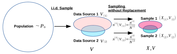
Figure 1: Sampling scheme for merged data from multiple sources with $J=2$.

The two-stage formulation is crucial in describing duplicated selection. A large sample is drawn from a population (sampling from population), and units are classified into one or more (sample) data sources. Next, subsamples are drawn without replacement from each data source (finite-population sampling) to generate multiple datasets. The sample at the first stage serves as a finite population to allow for repeated selection of the same units.

Information that statisticians have at their disposal is the $X$- and $V$-values of the selected items from different sources, membership information on (other) data sources to which selected items belong, and the realizations of $N^{(j)}$ and $n^{(j)}$. A special case where $V$-values are also available for non-sampled items is treated in Section 4.

Our framework covers a number of applications. Typical examples are opinion polls [9], public health surveillance [30], and health interview surveys [11] where data sources are lists of cell- and landline-phone users. Duplicated records in databases are important issues in business operations [28]. Scientific research has considered combining face-to-face, telephone and online surveys [15, 17]. Our setting also covers the situation where one data source is entirely contained in another. This case is highly useful for studying rare disease and rare exposure represented as smaller data sources [33, 35]. Applications include the synthesis of existing clinical and epidemiological studies with surveys, disease registries, and healthcare databases [12, 36, 45].

Despite scientific and financial benefits of data integration, many important models have never been studied in our setting due to the lack of probabilistic tools to study a dependent and biased sample with duplication. We address this issue by extending empirical process theory with applications to infinite-dimensional $M$-estimation in mind. This theory provides essential tools for the analysis of semi- and non-parametric inference (see e.g. [38, 58]). It originated in the study of the uniform law of large numbers (U-LLN) and the uniform central limit theorem (U-CLT) in the i.i.d. setting [10, 19, 20, 22, 23]. The i.i.d. assumption has been relaxed in several directions including triangular arrays [61, 62], martingale difference [40], Markov chains [2], and stationary processes [3]. The study of dependent empirical processes arising from complex sampling was initiated by [7] for stratified samples followed by [52]. Beyond stratified samples, [4] and [5] studied the U-CLT for rejective sampling and single stage sampling, respectively.

Our sampling scheme is markedly different from those in the above literature in important ways. A basic technique to analyze dependent empirical processes is to find a hidden (nearly) independent structure as seen in [4] that utilized similarity between independent Poisson sampling and rejective sampling. This method needs a simple dependence structure but our merged data have complex multitiered dependence: First, items within the same source are dependent due to sampling without replacement. Second, items across overlapping sources are dependent because they are potentially identical. Previous studies focused on dependence within a sample but our theory addresses dependence within and between samples at the same time. Another difference is that simple inverse probability weighting adopted in [4, 5, 7] is not valid in our setting. This technique corrects selection bias from data sources but does not account for bias from duplicated selection.

We build large sample theory on a novel weighted empirical process that integrates information from multiple sources. Our main contribution is the U-LLN and U-CLT over a class of functions. We only assume that an index set is Glivenko-Cantelli or Donsker as in [7, 52]. This implies that if the U-LLN or the U-CLT holds for the i.i.d. sample, the corresponding results hold for merged data without additional conditions. This formulation is of practical importance because fair comparison can be made between previous scientific conclusions from i.i.d. samples and the ones from the analysis of merged data without worrying about differences in assumptions. This generality makes a contrast with [4] that assumes the uniform entropy condition and [5] that assumes a priori the existence of the finite-dimensional CLT.

Another contribution is theory of infinite-dimensional $M$-estimation for merged data. Previous research tended to focus on the U-CLT with limited applications as a result (e.g. statistical functionals in [4, 5]), but the U-LLN and maximal inequalities are essential to obtain consistency and rates of convergence for $M$-estimators. We obtain a set of empirical process tools beyond the U-CLT, and derive consistency, rates of convergence, and asymptotic normality of our estimators. We obtain optimal calibration [16, 48] and optimal weights in our weighted empirical process that improve efficiency of our estimators. We study several examples including the Cox proportional hazards models [13] and illustrate the finite sample performance of our methods through numerical studies in several different scenarios.

Our theory can be viewed as a non-trivial extension of [7, 52] for stratified samples to overlapping “strata.” In stratified sampling, the i.i.d. sample from population is stratified and finite population sampling is carried out in each stratum. One may consider our sampling scheme as “stratified sampling” with non-negligible intersections among strata. The approach of [7, 52] is, however, not applicable to our setting due to issues of multitiered dependence and inverse probability weighting discussed above. In particular, their proof exploited the disjoint nature of strata and reduced weak convergence to multiple convergence within strata. This method addresses dependence within strata but does not cover dependence across “strata” arising from duplicated selection (see Section 3 for details). Note that our framework is more general than previously studied sampling designs including stratified sampling in that it accommodates those designs in place of finite population sampling. In the Appendix D, we treat stratified sampling at the second stage of sampling in the data integration context.

The rest of the paper is organized as follows. In Section 2, we introduce our weighted empirical process and discuss more on our sampling framework. We present the U-LLN and several variants of U-CLTs in Section 3. Calibration methods are treated in Section 4. We study infinite-dimensional $M$- and $Z$-estimation and their applications in Section 5. Finite sample properties of proposed methods are illustrated in numerical studies in Section 6. Section 7 discusses differences between our framework and those in sampling theory. All proofs and additional simulation are given in the Appendix.

2 Sampling and Empirical Process

We review basic settings and introduce our weighted empirical process.

2.1 Sampling

Let $R_{i}^{(j)}\in\{0,1\}$ be a sampling indicator from source $j$. Simple random sampling from each source is carried out independently. Thus, sampling indicators $(R_{1}^{(j)},\ldots,R_{N}^{(j)})$ and $(R_{1}^{(j^{\prime})},\ldots,R_{N}^{(j^{\prime})})$ with $j\neq j^{\prime}$ are conditionally independent given $V_{1},\ldots,V_{N}$. However, sampling indicators within the same source are not independent but are only exchangeable due to sampling without replacement. The unit that does not belong to source $j$ (i.e., $V_{i}\notin\mathcal{V}^{(j)}$) automatically has $R_{i}^{(j)}=0$. Throughout we denote inverse probability weighting by $R_{i}^{(j)}/\pi^{(j)}(V_{i})$ with convention $0/0=0$.

To enumerate units within a data source, we write e.g. $X_{(j),i}$ to mean the observation of $X$ for the unit $i$ in source $j$ with index $i$ going from 1 through $N^{(j)}$ (see e.g. 3.4). The limits of sampling probabilities are $\lim_{N\rightarrow\infty}\pi^{(j)}(v)=p^{(j)}I\{v\in\mathcal{V}^{(j)}\}$ where $p^{(j)}\geq c>0$ for some constant $c$. We assume $N$ is known. In the Appendix F, we consider the case of unknown $N$ which may be the case in practice. For additional notations, let $W=(X,U)\in\mathcal{X}\times\mathcal{U}\equiv\mathcal{W}$ with $W\sim\tilde{P}_{0}$. The conditional measure given membership in source $j$ is denoted as $P_{0}^{(j)}$, i.e., for measurable $A\subset\mathcal{W}$, $P_{0}^{(j)}(A)=\tilde{P}_{0}(A\cap\mathcal{V}^{(j)})/\nu^{(j)}$ where $\nu^{(j)}\equiv\tilde{P}_{0}(V\in\mathcal{V}^{(j)})$ is membership probability in source $j$. The conditional probability measure for $R_{i}^{(j)}$ given $N^{(j)},i=1,\ldots,N,j=1,\ldots,J$, is denoted as $P_{R,N}$. The probability measure $P^{\infty}$ is defined such that its projection of the first $N$ coordinates is $\tilde{P}_{0}^{N}\times P_{R,N}$.

2.2 Assumption of Unidentified Duplication

Duplicated items are not identified in our setting, which reflects the lack of communication between sampling procedures. Instead, we assume that we can identify additional data source membership of selected items by checking their $V$. This assumption is not too restrictive. For example, telephone surveys can ask an additional question whether to own both landline and cell phones. When medical studies are merged, comparison of inclusion and exclusion criteria suffices. Identifying duplication, on the other hand, produces unavoidable errors. Important identifiers such as names, addresses, and social security numbers are usually not disclosed for a privacy reason, and even these variables suffer typographical errors and inconsistent abbreviations [21, 60]. Correcting bias from imperfect record linkage requires a correctly specified model of linking errors [37, 39]. Our proposed method avoids these practical difficulties, and remains valid even when identification is possible.

2.3 Hartley-Type Empirical Process

The empirical measure is a fundamental object in empirical process theory. This cannot be computed in our setting because of non-selected items and unidentified duplicated selection. As an alternative, we propose to study Hartley’s estimator [25, 26] of a distribution function in place of the empirical measure.

Hartley’s estimator [25, 26] was originally proposed for estimation of population total and average in multiple-frame surveys in sampling theory where multiple samples are drawn from overlapping sampling frames. Viewing sampling frames as data sources in our context, Hartley’s estimator of the sample average $\mathbb{P}_{N}X$ of $X$ when $J=2$ is defined as

$$\mathbb{P}_{N}^{\textup{H}}X \equiv \frac{1}{N}\sum_{i=1}^{N}\left(\frac{R_{i}^{(1)}\rho^{(1)}(V_{i})}{\pi^{(1)}(V_{i})}+\frac{R_{i}^{(2)}\rho^{(2)}(V_{i})}{\pi^{(2)}(V_{i})}\right)X_{i},$$

where the weight function $\rho$ for duplicated selection is given by

$$\rho(v)=(\rho^{(1)}(v),\rho^{(2)}(v))\equiv\left\{\begin{array}[]{ll}(1,0)&\quad\mbox{if}\quad v\in\mathcal{V}^{(1)}\mbox{ and }v\notin\mathcal{V}^{(2)},\\ (0,1)&\quad\mbox{if}\quad v\notin\mathcal{V}^{(1)}\mbox{ and }v\in\mathcal{V}^{(2)},\\ (c^{(1)},c^{(2)})&\quad\mbox{if}\quad v\in\mathcal{V}^{(1)}\cap\mathcal{V}^{(2)},\\ \end{array}\right.$$

for positive constants $c^{(1)},c^{(2)}$ with $c^{(1)}+c^{(2)}=1$. Duplicated selection and missing observations are properly addressed by the weight function $\rho(v)$ and the inverse probability weights respectively. In fact, this estimator is unbiased for $E(X)$ because $\rho^{(1)}(v)+\rho^{(2)}(v)=1$ for all $v$ and $E[R^{(j)}_{i}|X_{i},V_{i},N^{(j)},n^{(j)}]=\pi^{(j)}(V_{i})$. Moreover, identification of duplicated items is not necessary to compute this estimator because the two sums

$$\mathbb{P}_{N}^{\textup{H}}X=\frac{1}{N}\sum_{i=1}^{N}\frac{R_{i}^{(1)}\rho^{(1)}(V_{i})}{\pi^{(1)}(V_{i})}X_{i}+\frac{1}{N}\sum_{i=1}^{N}\frac{R_{i}^{(2)}\rho^{(2)}(V_{i})}{\pi^{(2)}(V_{i})}X_{i},$$ (2.2)

in $\mathbb{P}_{N}^{\textup{H}}X$ can be computed separately based on each subsample.

Motivated by Hartley’s estimator, we define the Hartley-type empirical measure (H-empirical measure) for $J=2$ by

$$\mathbb{P}_{N}^{\textup{H}} \equiv \frac{1}{N}\sum_{i=1}^{N}\left(\frac{R_{i}^{(1)}\rho^{(1)}(V_{i})}{\pi^{(1)}(V_{i})}+\frac{R_{i}^{(2)}\rho^{(2)}(V_{i})}{\pi^{(2)}(V_{i})}\right)\delta_{(X_{i},V_{i})}.$$

This is an unbiased estimator of the empirical measure $\mathbb{P}_{N}\equiv N^{-1}\sum_{i=1}^{N}\delta_{(X_{i},V_{i})}$ given $(X_{i},V_{i}),i=1,\ldots,N$. Note, however, that $\mathbb{P}_{N}^{\textup{H}}$ is not a probability measure since point masses do not add up to 1 in general. The Hartley-type empirical process (H-empirical process) is defined by

$$\mathbb{G}_{N}^{\textup{H}}=\sqrt{N}(\mathbb{P}_{N}^{\textup{H}}-\tilde{P}_{0}).$$

When there are more than two sources, we define the weight function $\rho=(\rho^{(1)},\ldots,\rho^{(J)}):\mathcal{V}\mapsto[0,1]^{J}$ that is constant on a mutually exclusive subset of $\mathcal{V}$ determined by $\mathcal{V}^{(j)}$’s:

$$\rho^{(j)}(v)=\left\{\begin{array}[]{ll}1,&v\in\mathcal{V}^{(j)}\cap\left(\cup_{m\neq j}\mathcal{V}^{(m)}\right)^{c},\\ c^{(j)}_{k_{1},\ldots,k_{l}},&v\in\mathcal{V}^{(j)}\cap\left(\cap_{m=1}^{l}\mathcal{V}^{(k_{m})}\right)\cap\left(\cup_{m\notin\{j,k_{1},\ldots,k_{l}\}}\mathcal{V}^{(m)}\right)^{c},\\ 0,&v\notin\mathcal{V}^{(j)},\\ \end{array}\right.$$

with $j,k_{1},\ldots,k_{l}$ all different and $\sum_{j=1}^{J}\rho^{(j)}(v)=1$. The H-empirical measure is defined by

$$\mathbb{P}_{N}^{\textup{H}}\equiv\frac{1}{N}\sum_{i=1}^{N}\sum_{j=1}^{J}\frac{R_{i}^{(j)}\rho^{(j)}(V_{i})}{\pi^{(j)}(V_{i})}\delta_{(X_{i},V_{i})}.$$

and the H-empirical process is defined by $\mathbb{G}_{N}^{\textup{H}}=\sqrt{N}(\mathbb{P}_{N}^{\textup{H}}-\tilde{P}_{0})$.

Let $\mathcal{F}$ be a class of measurable functions on $(\mathcal{X},\mathcal{A})$ that serves as the index set for the H-empirical process. As a stochastic process indexed by $\mathcal{F}$, $\mathbb{G}_{N}^{\textup{H}}$ evaluated at $f\in\mathcal{F}$ is a random variable $\mathbb{G}_{N}^{\textup{H}}f=\sqrt{N}(\mathbb{P}_{N}^{\textup{H}}-\tilde{P}_{0})f=\sqrt{N}(\mathbb{P}_{N}^{\textup{H}}f-\tilde{P}_{0}f)$ where $\tilde{P}_{0}f$ is the expectation of $f(X)$ under $\tilde{P}_{0}$, and $\mathbb{P}_{N}^{\textup{H}}f$ is the “expectation” of $f(X)$ under $\mathbb{P}_{N}^{\textup{H}}$ given by

$$\mathbb{P}_{N}^{\textup{H}}f\equiv\frac{1}{N}\sum_{i=1}^{N}\sum_{j=1}^{J}\frac{R_{i}^{(j)}\rho^{(j)}(V_{i})}{\pi^{(j)}(V_{i})}f(X_{i}).$$

We often omit variables of a function in “expectations” as in $\mathbb{P}_{N}^{\textup{H}}f$ and $\mathbb{G}_{N}^{\textup{H}}f$.

3 Limit Theorems: Uniform WLLN and CLT

The U-LLN and U-CLT for the H-empirical process lay the groundwork for the analysis of merged data from multiple sources. The critical issue for establishing these theorems is multitiered dependence. This is not a difficult problem in the finite-population framework where only sampling indicators $R^{(j)}_{i}$ are random. For example, the two terms of $\mathbb{P}_{N}^{\textup{H}}X$ in (2.2) are independent in this framework, and each admits a finite-population CLT (e.g. [24]) to yield the sum of independent normal random variables as a limit [43]. A similar idea appears in the analysis of stratified samples. For the derivation of the U-CLT, [7] decomposed their weighted empirical process into stratum-wise empirical processes and showed their conditional weak convergence to independent Gaussian processes given data. Because strata do not overlap unlike our case, conditional independence automatically becomes unconditional to complete their proof. Unfortunately, this conditional argument is not valid in our setting due to dependence across overlapping data sources.

Our approach consists of two key ideas: (1) the decomposition of the H-empirical process into data sources with centering by appropriate variables, and (2) bootstrap asymptotics for establishing unconditional asymptotic normality. Our decomposition ensures unconditional independence, and bootstrap asymptotics bridges unconditional and conditional convergence.

Our decomposition emulates two stages of the sampling procedure:

$$\mathbb{G}_{N}^{\textup{H}}=\sqrt{N}(\mathbb{P}_{N}^{\textup{H}}-\tilde{P}_{0})=\sqrt{N}(\mathbb{P}_{N}-\tilde{P}_{0})+\sqrt{N}(\mathbb{P}_{N}^{\textup{H}}-\mathbb{P}_{N}).$$

The first term is the empirical process $\mathbb{G}_{N}=\sqrt{N}(\mathbb{P}_{N}-\tilde{P}_{0})$ for the i.i.d. sample which corresponds to sampling from population at the first stage. This process weakly converges to the Brownian bridge by the U-CLT for the i.i.d. sample. The second term corresponding to sampling from data sources is further decomposed. Note that $\mathbb{P}_{N}f=\sum_{j=1}^{J}\mathbb{P}_{N}\rho^{(j)}(V)f(X)$ by the fact that $\sum_{j=1}^{J}\rho^{(j)}(v)=1$ for every $v$. Combining this with the decomposition of $\mathbb{P}_{N}^{\textup{H}}$ in (2.2) with a general $J$ yields

$$(\mathbb{P}_{N}^{\textup{H}}-\mathbb{P}_{N})f = \sum_{j=1}^{J}\frac{1}{N}\sum_{i=1}^{N}\left(\frac{R^{(j)}_{i}}{\pi^{(j)}(V_{i})}-1\right)\rho^{(j)}(V_{i})f(X_{i})$$

$$\equiv \sum_{j=1}^{J}(\mathbb{P}_{N}^{\textup{H},(j)}-\mathbb{P}_{N})\rho^{(j)}f.$$

As in the finite-population framework, the conditional covariance of $(\mathbb{P}_{N}^{\textup{H},(j)}-\mathbb{P}_{N})\rho^{(j)}f$ with different $j$’s is zero given data $(X_{i},V_{i}),i=1,\ldots,N,$ because sampling from different data sources (i.e., $R^{(j)}$s and $R^{(j^{\prime})}$s) is independent. Moreover, their conditional expectations given data are also zero because $E[R^{(j)}_{i}|X_{i},V_{i},N^{(j)},n^{(j)}]=\pi^{(j)}(V_{i})$. It follows from the total law of covariance (i.e., $\textup{Cov}(X,Y)=E[\textup{Cov}(X,Y|Z)]+\textup{Cov}(E[X|Z],E[Y|Z])$) that any two of summands in the last display are uncorrelated. The same argument applies to the relationship between each summand and $\sqrt{N}(\mathbb{P}_{N}-\tilde{P}_{0})f$. Hence we obtain the decomposition of $\mathbb{G}_{N}^{\textup{H}}$ into $J+1$ uncorrelated pieces:

$$\mathbb{G}_{N}^{\textup{H}}f=\sqrt{N}(\mathbb{P}_{N}-\tilde{P}_{0})f+\sum_{j=1}^{J}\sqrt{N}(\mathbb{P}_{N}^{\textup{H},(j)}-\mathbb{P}_{N})\rho^{(j)}f.$$

If we show each summand converges to a Gaussian process, the limiting process of $\mathbb{G}_{N}^{\textup{H}}$ is the sum of $J+1$ independent Gaussian processes.

To establish weak convergence of the second term in the last display, we adopt the bootstrap asymptotic theory. The key observation is to view sampling from a data source $j$ as a single realization of the $m$-out-of-$n$ bootstrap with $m=n^{(j)}$ and $n=N^{(j)}$ where a bootstrap sample of size $m$ is drawn from a sample of size $n$ without replacement. To see this, rewrite $(\mathbb{P}_{N}^{\textup{H},(j)}-\mathbb{P}_{N})\rho^{(j)}f$ by $(N^{(j)}/N)(\hat{\mathbb{P}}^{(j)}_{n^{(j)}}-\mathbb{P}^{(j)}_{N^{(j)}})\rho^{(j)}f$ where

$$\hat{\mathbb{P}}^{(j)}_{n^{(j)}}\equiv\frac{1}{n^{(j)}}\sum_{i=1}^{N^{(j)}}R^{(j)}_{(j),i}\delta_{(X_{(j),i},V_{(j),i})},\qquad\mathbb{P}^{(j)}_{N^{(j)}}\equiv\frac{1}{N^{(j)}}\sum_{i=1}^{N^{(j)}}\delta_{(X_{(j),i},V_{(j),i})}.$$ (3.4)

Here we enumerate the items within data source $j$. Focusing on source $j$, $\mathbb{P}^{(j)}_{N^{(j)}}\rho^{(j)}f$ is the sample mean of $\rho^{(j)}(V)f(X)$ before sampling at the second stage while $\hat{\mathbb{P}}^{(j)}_{n^{(j)}}\rho^{(j)}f$ is the sample mean after sampling. In view of the $m$-out-of-$n$ bootstrap, the former is an average in the original sample while the latter is a bootstrap average, and hence their difference is expected to yield asymptotic normality with appropriate scaling. Although $m/n=n^{(j)}/N^{(j)}\rightarrow p^{(j)}\neq 0$ unlike the usual $m$-out-of-$n$ bootstrap method, asymptotics in our case can be treated as the special case of the exchangeably weighted bootstrap studied by [46]. Theory of [46] emphasized conditional weak convergence, but it is not difficult to extend their proof to unconditional one. Accordingly we obtain the sum of independent Gaussian processes as the limit of $\mathbb{G}_{N}^{\textup{H}}$. In the Appendix A, we make this heuristic argument rigorous.

Below we write $P^{*}$ and $E^{*}$ to mean outer probability of $P^{\infty}$ and expectation with respect to $P^{*}$. Since empirical process theory concerns the supremum of random elements, we use these notations to take care of measurability issues. For more details, see Section 1.2 of [58]. A reader not interested in technical details can replace these by $\tilde{P}_{0}$ and $E$ without harm.

3.1 Uniform Law of Large Numbers

The U-LLN holds for the empirical measure $\mathbb{P}_{N}$ in the i.i.d. setting if the index set $\mathcal{F}$ is a Glivenko-Cantelli class (see e.g. p.81 of [58]). This Glivenko-Cantelli property is sufficient for the U-LLN for merged data from multiple sources. The following result is obtained by applying the bootstrap U-LLN [58] to our decomposition of $\mathbb{G}_{N}^{\textup{H}}$.

Theorem 3.1.

Suppose that $\mathcal{F}$ is $P_{0}$-Glivenko-Cantelli. Then

$$\lVert\mathbb{P}_{N}^{\textup{H}}-\tilde{P}_{0}\rVert_{\mathcal{F}}=\sup_{f\in\mathcal{F}}|(\mathbb{P}_{N}^{\textup{H}}-\tilde{P}_{0})f|\rightarrow_{P^{*}}0,$$

where $\lVert\ell\rVert_{\mathcal{F}}=\sup_{f\in\mathcal{F}}|\ell(f)|$ for a functional $\ell$ on $\mathcal{F}$.

3.2 Uniform Central Limit Theorem

The empirical process $\mathbb{G}_{N}$ in the i.i.d. setting weakly converges to a Gaussian process if the index set $\mathcal{F}$ is a Donsker class (see e.g. p.81 of [58]). This Donsker property is sufficient for the U-CLT for the H-empirical process $\mathbb{G}_{N}^{\textup{H}}$. This is an expected consequence from bootstrap asymptotics which does not need additional conditions.

Theorem 3.2.

Suppose that $\mathcal{F}$ is $P_{0}$-Donsker. Then

$$\mathbb{G}_{N}^{\textup{H}}(\cdot)\rightsquigarrow\mathbb{G}^{\textup{H}}(\cdot)\equiv\mathbb{G}(\cdot)+\sum_{j=1}^{J}\sqrt{\nu^{(j)}}\sqrt{\frac{1-p^{(j)}}{p^{(j)}}}\mathbb{G}^{(j)}(\rho^{(j)}\cdot)$$

in the class $\ell^{\infty}(\mathcal{F})$ of uniformly bounded functionals on $\mathcal{F}$ where the $P_{0}$-Brownian bridge process $\mathbb{G}$ and the $P_{0}^{(j)}$-Brownian bridge processes $\mathbb{G}^{(j)}$ are independent. The covariance function $\upsilon(\cdot,\cdot)=\textup{Cov}(\mathbb{G}^{\textup{H}}\cdot,\mathbb{G}^{\textup{H}}\cdot)$ on $\mathcal{F}\times\mathcal{F}$ is

$$\upsilon(f,g)=\textup{Cov}_{0}(f,g)+\sum_{j=1}^{J}\nu^{(j)}\frac{1-p^{(j)}}{p^{(j)}}\textup{Cov}_{0}^{(j)}(\rho^{(j)}f,\rho^{(j)}g).$$

where $\textup{Cov}_{0}$ and $\textup{Cov}_{0}^{(j)}$ are covariances under $P_{0}$ and $P_{0}^{(j)}$ respectively.

The asymptotic variance here admits natural interpretations. Consider $\mathbb{G}_{N}^{\textup{H}}f$ for estimation of $P_{0}f$ for instance. Its asymptotic variance is

$$\textup{AV}(\mathbb{G}_{N}^{\textup{H}}f)=\underbrace{\textup{Var}_{0}\{f(X)\}}_{\mbox{population variance}}+\sum_{j=1}^{J}\underbrace{\nu^{(j)}\frac{1-p^{(j)}}{p^{(j)}}\textup{Var}_{0}^{(j)}\{\rho^{(j)}(V)f(X)\}}_{\mbox{design variance from source $j$}},$$

where $\textup{Var}_{0}(f)=\textup{Cov}_{0}(f,f)$ and $\textup{Var}_{0}^{(j)}(f)=\textup{Cov}^{(j)}_{0}(f,f)$. The first and second terms correspond to sampling from population and data sources respectively. If we would obtain the i.i.d. sample instead, the asymptotic variance is only the first term $\textup{Var}_{0}\{f(X)\}$. This can be obtained from our formula if we would sample all items from each data source (i.e., $p^{(j)}=1$). This implies that as long as we sample all the items at the second stage, combining multiple datasets does not increase the difficulty of estimation. If data source $j$ is large (i.e., $\tilde{P}_{0}(V\in\mathcal{V}^{(j)})=\nu^{(j)}$ is large), its contribution to asymptotic variance becomes larger. Each quantity in the variance formula is easily estimated by Hartleys’ estimator of moments (see also the Appendix G for variance estimators for several regression models).

Remark 3.1.

In Theorems 3.1 and 3.2, we assume Glivenko-Cantelli and Donsker properties of $\mathcal{F}$ with respect to $P_{0}$ in order to emphasize that these properties in the i.i.d. setting are sufficient for our setting. A brief inspection of our proof reveals that our theorems hold valid for $\tilde{P}_{0}$-Glivenko-Cantelli and $\tilde{P}_{0}$-Donsker classes of functions defined on $\mathcal{W}=\mathcal{X}\times\mathcal{U}$.

3.2.1 Finite-Population sampling

Finite-population sampling concerns randomness only from the selection of units, and is often of interest in sampling theory. As expected from our interpretation of asymptotic variance in Theorem 3.2, we only obtain design variance from sources in this framework.

Corollary 3.1.

Suppose that $\mathcal{F}$ is $P_{0}$-Donsker. Then

$$\mathbb{G}_{N}^{\textup{H,fin}}(\cdot)\equiv\sqrt{N}(\mathbb{P}_{N}^{\textup{H}}-\mathbb{P}_{N})(\cdot)\rightsquigarrow\mathbb{G}^{\textup{H,fin}}(\cdot)\equiv\sum_{j=1}^{J}\sqrt{\nu^{(j)}}\sqrt{\frac{1-p^{(j)}}{p^{(j)}}}\mathbb{G}^{(j)}(\rho^{(j)}\cdot)$$

in $\ell^{\infty}(\mathcal{F})$ conditionally on $(X_{1},V_{1}),(X_{2},V_{2})\ldots,$ with the covariance function $\upsilon^{\textup{fin}}(\cdot,\cdot)=\textup{Cov}(\mathbb{G}^{\textup{H,fin}}\cdot,\mathbb{G}^{\textup{H,fin}}\cdot)$ on $\mathcal{F}\times\mathcal{F}$given by

$$\upsilon^{\textup{fin}}(f,g)=\sum_{j=1}^{J}\nu^{(j)}\frac{1-p^{(j)}}{p^{(j)}}\textup{Cov}_{0}^{(j)}(\rho^{(j)}f,\rho^{(j)}g).$$

3.2.2 Bernoulli Sampling

Sampling without replacement is often replaced by Bernoulli sampling for mathematical convenience. To see its consequence, we consider Bernoulli sampling within sources where selections from source $j$ are i.i.d. Bernoulli$(p^{(j)})$. Data from the same source then become independent, but dependence remains between datasets from overlapping sources. We write $\mathbb{G}_{N}^{\textup{H,Ber}}$ for the H-empirical process in this case.

Theorem 3.3.

Suppose that $\mathcal{F}$ is $P_{0}$-Donsker. Then $\mathbb{G}_{N}^{\textup{H,Ber}}\rightsquigarrow\mathbb{G}^{\textup{H,Ber}}$ in $\ell^{\infty}(\mathcal{F})$ where $\mathbb{G}^{\textup{H,Ber}}$ is the zero-mean Gaussian process $\mathbb{G}^{\textup{H,Ber}}$ with covariance function $\upsilon^{\textup{Ber}}(\cdot,\cdot)=\textup{Cov}(\mathbb{G}^{\textup{H,Ber}}\cdot,\mathbb{G}^{\textup{H,Ber}}\cdot)$ on $\mathcal{F}\times\mathcal{F}$ given by

$$\upsilon^{\textup{Ber}}(f,g)=\textup{Cov}_{0}(f,g)+\sum_{j=1}^{J}\nu^{(j)}\frac{1-p^{(j)}}{p^{(j)}}P_{0}^{(j)}\left\{(\rho^{(j)})^{2}fg\right\}.$$

Bernoulli sampling yields larger asymptotic variance than sampling without replacement. As expected from the decomposition of the asymptotic variance, the difference appears only in the design variances.

Corollary 3.2 (Finite-Population Correction).

The asymptotic variance is smaller when subsamples from sources are obtained from sampling without replacement than from Bernoulli sampling. In particular,

$$\textup{AV}(\mathbb{G}_{N}^{\textup{H}}f)=\textup{AV}(\mathbb{G}_{N}^{\textup{H,Ber}}f)-\sum_{j=1}^{J}\nu^{(j)}\frac{1-p^{(j)}}{p^{(j)}}\{P_{0}^{(j)}\rho^{(j)}(V)f(X)\}^{2}.$$

3.2.3 Optimal $\rho$

We derive the optimal weight function $\rho$ based on our U-CLT. We propose the use of the optimal $\rho$ under Bernoulli sampling which only involves $p^{(j)}$ determined by design. The optimal $\rho$ under sampling without replacement involves an estimand itself and should differ from parameter to parameter. We show the optimal choice under Bernoulli sampling works well under sampling without replacement in simulation studies in Section 5.

Proposition 3.1 (Optimal $\rho$ under Bernoulli Sampling).

Let $f:\mathcal{X}\rightarrow\mathbb{R}^{k}$ be arbitrary with $P_{0}f^{2}<\infty$. Let $od(p)=(1-p)/p$. When $J=2$, the optimal function $\rho$ that minimizes the asymptotic variance of $\mathbb{G}^{\textup{H,Ber}}_{N}f$ has

$$c^{(1)}=\frac{od(p^{(2)})}{od(p^{(1)})+od(p^{(2)})},\quad c^{(2)}=\frac{od(p^{(1)})}{od(p^{(1)})+od(p^{(2)})}.$$

When $J\geq 2$, the optimal function $\rho$ that minimizes the asymptotic variance of $\mathbb{G}^{\textup{H,Ber}}_{N}f$ has (1) $c^{(j)}_{k_{1},\ldots,k_{l}}=0$ if $p^{(j)}<1$ and $p^{(k_{m})}=1$ for some $m$, (2) arbitrary $c^{(j)}_{k_{1},\ldots,k_{l}}$ if $p^{(j)}=1$, and (3)

$$c^{(j)}_{k_{1},\ldots,k_{l}}=\frac{\prod_{m=1}^{l}od(p^{(k_{m})})}{\prod_{m=1}^{l}od(p^{(k_{m})})+od(p^{(j)})\sum_{n=1}^{l}\prod_{m=1}^{l}od(p^{(k_{m})})/od(p^{(k_{n})})},$$

if $p^{(j)},p^{(k_{m})}<1,m=1,\ldots,l$.

For sampling without replacement, we treat the case $J=2$ only. The general case can be similarly derived via quadratic programming.

Proposition 3.2 (Optimal $\rho$ under Sampling without Replacement).

Let $f:\mathcal{X}\rightarrow\mathbb{R}^{k}$ be a function with $P_{0}f^{2}<\infty$. Let $Y_{f}\equiv f(X)I\{V\in\mathcal{V}^{(1)}\cap\{\mathcal{V}^{(2)}\}^{c}\}$ and $Z_{f}\equiv f(X)I\{V\in\mathcal{V}^{(1)}\cap\mathcal{V}^{(2)}\}$. Define

$$c_{f}\equiv\frac{-\nu^{(1)}od(p^{(1)})P_{0}^{(1)}Y_{f}P_{0}^{(1)}Z_{f}\ +\nu^{(2)}od(p^{(2)})\left\{P_{0}^{(2)}Y_{f}P_{0}^{(2)}Z_{f}-\textup{Var}_{0}^{(2)}(Z_{f})\right\}}{\nu^{(1)}od(p^{(1)})\textup{Var}_{0}^{(1)}(Z_{f})+\nu^{(2)}od(p^{(2)})\textup{Var}_{0}^{(2)}(Z_{f})}.$$

When $J=2$, the optimal function $\rho$ that minimizes the asymptotic variance of $\mathbb{G}^{\textup{H}}_{N}f$ has $c^{(1)}=0\vee c_{f}\wedge 1$ and $c^{(2)}=1-c$.

In a finite-population framework, [41] derived optimal $\rho$ for general complex surveys. Their optimal $\rho$ agrees with ours under Bernoulli sampling, but they differ under sampling without replacement. The difference is due to their probabilistic framework where [41] minimizes variance of $\mathbb{P}_{N}^{\textup{H}}f$ (which is zero in the limit) rather than the asymptotic variance of $\mathbb{G}_{N}^{\textup{H}}f$.

4 Calibration

The H-empirical process is computed from selected units only. If information on auxiliary variables $V$ are available for non-selected units, calibration methods improve efficiency of our estimator. The key idea for calibration is that a statistic computed from sampled units (e.g. $\mathbb{P}_{N}^{\textup{H}}V$) is approximately equal to a statistic computed from all units (e.g. $\mathbb{P}_{N}V$). Adjusting weights in $\mathbb{P}_{N}^{\textup{H}}$ that induce similarity between two statistics makes selected units more representative of the population. Different methods use different pairs of two statistics. Below, we first introduce the extension of [47] to a general $J\geq 2$ and then propose our method.

The original calibration [16] ((2.3) of p. 377) equates the Horvitz-Thompson estimator [29] of $\tilde{P}_{0}V$ and sample average $\mathbb{P}_{N}V$ in order to improve the Horvitz-Thompson estimator of $P_{0}X$. Along the same line, [47] imposed a constraint on Hartley’s estimator $\mathbb{P}_{N}^{\textup{H}}V$ and sample average $\mathbb{P}_{N}V$ to improve $\mathbb{P}_{N}^{\textup{H}}X$ when $J=2$. For a general $J$ we consider as its extension the following calibration equation:

$$\mathbb{P}_{N}^{\textup{H}}G(V^{T}\alpha)V=\mathbb{P}_{N}V,$$ (4.5)

with a solution $\hat{\alpha}_{N}^{\textup{c}}$. Here $G$ is a fixed function (see [16] for some choice of $G$). Using $G(V^{T}\hat{\alpha}_{N}^{\textup{c}})$, the calibrated H-empirical measure is defined as

$$\mathbb{P}_{N}^{\textup{H,c}}(\cdot)\equiv\mathbb{P}_{N}^{\textup{H}}G(V^{T}\hat{\alpha}_{N}^{\textup{c}})(\cdot)=\frac{1}{N}\sum_{i=1}^{N}\sum_{j=1}^{J}\frac{R^{(j)}_{i}\rho^{(j)}(V_{i})}{\pi^{(j)}(V_{i})}G(V_{i}^{T}\hat{\alpha}_{N}^{\textup{c}})\delta_{(X_{i},V_{i})},$$

and the calibrated H-empirical process is defined as $\mathbb{G}_{N}^{\textup{H,c}}\equiv\sqrt{N}(\mathbb{P}_{N}^{\textup{H,c}}-\tilde{P}_{0})$. Other variants in [47] can be extended by changing the range of summation. For example, if we replace $V$ by a vector with elements $VI_{\mathcal{V}^{(j)}}(V),j=1,\ldots,J,$ in (4.5), we obtain data-source-specific calibration

$$\frac{1}{N}\sum_{i:V_{i}\in\mathcal{V}^{(j)}}\sum_{j=1}^{J}\frac{R_{i}^{(j)}\rho^{(j)}(V_{i})}{\pi^{(j)}(V_{i})}G(V_{i}^{T}\alpha^{(j)})V_{i}=\frac{1}{N}\sum_{i:V_{i}\in\mathcal{V}^{(j)}}V_{i},\quad j=1,\ldots,J.$$

The left-hand is computed from all selected units that belong to source $j$.

Our proposed method exploits the asymptotic variance formula $\upsilon(f,f)$ in Theorem 3.2. We target the reduction of design variances in

$$\textup{Var}_{0}^{(j)}\{\rho^{(j)}(V)f(X)\}=P_{0}^{(j)}\{\rho^{(j)}(V)f(X)-P_{0}^{(j)}\rho^{(j)}(V)f(X)\}^{\otimes 2}.$$

The key observations are (1) the conditional variance is obtained from the sample from the same source (units with $R^{(j)}=1$), and (2) variables of interest are $\rho^{(j)}(V)f(X)-P_{0}^{(j)}\rho^{(j)}(V)f(X)$. Our method is thus characterized by the following three points: (1) calibration is carried out within a subsample from the same source, (2) variables used are $\rho^{(j)}(V)V$ with centering, and (3) Horvitz-Thompson estimators are equated with sample averages. To be specific, we propose the sample-specific calibration equation

$$\frac{1}{N^{(j)}}\sum_{i:V_{i}\in\mathcal{V}^{(j)}}\frac{R_{i}^{(j)}G^{(j)}_{\alpha^{(j)}}(V_{i})}{\pi^{(j)}(V_{i})}\left\{\rho^{(j)}(V_{i})V_{i}-\mathbb{P}_{N^{(j)}}^{(j)}\rho^{(j)}(V)V\right\}=0,$$ (4.6)

$j=1,\ldots,J$ with solution $\hat{\alpha}_{N}^{\textup{sc}}=(\hat{\alpha}_{N}^{\textup{sc},(1)},\ldots,\hat{\alpha}_{N}^{\textup{sc},(J)})^{T}$ where

$$G^{(j)}_{\alpha}(v)\equiv G\left[\left\{\rho^{(j)}(v)v-\mathbb{P}_{N^{(j)}}^{(j)}\rho^{(j)}(V)V\right\}^{T}\alpha^{(j)}\right].$$

The right-hand side of (4.6) is the average of empirically centered variables, and hence equals zero. The left-hand side is computed from selected items from source $j$ in contrast to data-source-specific calibration that uses all items sampled from both source $j$ and its overlapping sources. We define the H-empirical measure with sample-specific calibration by

$$\mathbb{P}_{N}^{\textup{H,sc}} \equiv \frac{1}{N}\sum_{i=1}^{N}\sum_{j=1}^{J}\frac{R_{i}^{(j)}\rho^{(j)}(V_{i})}{\pi^{(j)}(V_{i})}G^{(j)}_{\hat{\alpha}^{\textup{sc},(j)}_{N}}(V_{i})\delta_{(X_{i},V_{i})},$$

and the corresponding H-empirical process by $\mathbb{G}_{N}^{\textup{H,sc}}\equiv\sqrt{N}(\mathbb{P}_{N}^{\textup{H,sc}}-\tilde{P}_{0})$.

We assume the following condition for calibration methods.

Condition 4.1.

(a) $\hat{\alpha}_{N}^{\textup{c}}$ and $\hat{\alpha}_{N}^{\textup{sc}}$ are solutions of (4.5) and (4.6).

(b) $V\in\mathbb{R}^{k}$ has bounded support with $\mathcal{V}^{(j)}\neq\{0\},j=1,\ldots,J$.

(c) $G$ is a strictly increasing, continuously differentiable, bounded function on $\mathbb{R}$ such that $G(0)=1$. Its derivative $\dot{G}$ is strictly positive and bounded.

(d) $\tilde{P}_{0}V^{\otimes 2}$ and every $\textup{Var}_{0}^{(j)}\{\rho^{(j)}(V)V\}$ satisfying $P^{(j)}_{0}\rho^{(j)}(V)>0$ are finite and positive definite.

Condition 4.1 (a) ensures the existence of solutions to calibration equations. Under conditions (b)-(d), probability of their existence with the choice $G(x)=1+x$ tends to 1 as $N\rightarrow\infty$. When $V$ is bounded, $G(x)=1+x$ can be considered as a bounded function that satisfies (c). In this case,

$$\hat{\alpha}^{\textup{sc}(j)}_{N}=\left\{\frac{1}{N^{(j)}}\sum_{i:V_{i}\in\mathcal{V}^{(j)}}\frac{R_{i}^{(j)}}{\pi^{(j)}(V_{i})}\left(V^{\rho^{(j)}}_{i}\right)^{\otimes 2}\right\}^{-1}\frac{1}{N^{(j)}}\sum_{i:V_{i}\in\mathcal{V}^{(j)}}\frac{R_{i}^{(j)}}{\pi^{(j)}(V_{i})}V^{\rho^{(j)}}_{i}$$

where $V_{i}^{\rho^{(j)}}\equiv\rho^{(j)}(V_{i})V_{i}-\mathbb{P}_{N^{(j)}}^{(j)}\rho^{(j)}(V)V$. The probability of the existence of the matrix inverse above tends to 1 due to (d). A similar argument applies to $\hat{\alpha}_{N}^{\textup{c}}$. Note that the choice of $G$ does not affect the limiting processes in the uniform CLT for calibrated H-empirical processes below.

Theorem 4.1.

Suppose $\mathcal{F}$ is $P_{0}$-Donsker with $\lVert P_{0}\rVert_{\mathcal{F}}<\infty$. Under Condition 4.1,

$$\mathbb{G}_{N}^{\textup{H,c}}(\cdot)\rightsquigarrow\mathbb{G}^{\textup{H,c}}(\cdot)\equiv\mathbb{G}(\cdot)+\sum_{j=1}^{J}\sqrt{\nu^{(j)}}\sqrt{\frac{1-p^{(j)}}{p^{(j)}}}\mathbb{G}^{(j)}(\rho^{(j)}I-Q_{\textup{c}}^{(j)})(\cdot),$$

$$\mathbb{G}_{N}^{\textup{H,sc}}(\cdot)\rightsquigarrow\mathbb{G}^{\textup{H,sc}}(\cdot)\equiv\mathbb{G}(\cdot)+\sum_{j=1}^{J}\sqrt{\nu^{(j)}}\sqrt{\frac{1-p^{(j)}}{p^{(j)}}}\mathbb{G}^{(j)}(\rho^{(j)}I-Q_{\textup{sc}}^{(j)})(\cdot),$$

in $\ell^{\infty}(\mathcal{F})$. Here $\mathbb{G}$ and $\mathbb{G}^{(j)}$ are the same as in Theorem 3.2, $I$ is the identity map, and $Q_{\textup{c}}^{(j)}$ and $Q_{\textup{sc}}^{(j)}$ are maps from the class of functions on $\mathcal{X}$ to the class of linear maps on $\mathcal{V}$ defined by

$$Q_{\textup{c}}^{(j)}(f)[v]=\tilde{P}_{0}(f(X)V^{T})\{\tilde{P}_{0}V^{\otimes 2}\}^{-1}\rho^{(j)}(v)v,$$

$$Q_{\textup{sc}}^{(j)}(f)[v]=P_{0}^{(j)}\{\rho^{(j)}(V)f(X)(\rho^{(j)}(V)V-P_{0}^{(j)}\rho^{(j)}(V)V)^{T}\}$$

$$\qquad\times\left\{\textup{Var}_{0}^{(j)}\left(\rho^{(j)}(V)V\right)\right\}^{-1}\left\{\rho^{(j)}(v)v-P_{0}^{(j)}\rho^{(j)}(V)V\right\}I\{v\in\mathcal{V}^{(j)}\}.$$

Covariance functions $\upsilon^{\#}(\cdot,\cdot)=\textup{Cov}(\mathbb{G}^{\textup{H},\#}\cdot,\mathbb{G}^{\textup{H},\#}\cdot)$ on $\mathcal{F}\times\mathcal{F},\#\in\{\textup{c,sc}\}$ are

$$\upsilon^{\#}(f,g)=\textup{Cov}_{0}(f,g)+\sum_{j=1}^{J}\nu^{(j)}\frac{1-p^{(j)}}{p^{(j)}}\textup{Cov}_{0}^{(j)}\left(\rho^{(j)}f-Q_{\#}^{(j)}(f),\rho^{(j)}g-Q_{\#}^{(j)}(g)\right).$$

To compare above methods, define the class $\mathcal{C}$ of estimators of $P_{0}f$ for arbitrary $f$ with $P_{0}f^{\otimes 2}<\infty$ whose asymptotic variance takes the form of

$$\textup{Var}_{0}\{f(X)\}+\sum_{j=1}^{J}\nu^{(j)}\frac{1-p^{(j)}}{p^{(j)}}\textup{Var}_{0}^{(j)}\left[\rho^{(j)}(V)f(X)-L^{(j)}_{f}\left\{\rho^{(j)}(V)V\right\}\right]$$

where $L^{(j)}_{f}(v)$ is a linear function of $v$ that depends on $f$. Note that calibration and the sample-specific calibration have $L^{(j)}_{f}\{\rho^{(j)}(v)v\}=Q_{\textup{c}}^{(j)}(f)[v]$ and $L^{(j)}_{f}\{\rho^{(j)}(v)v\}=Q_{\textup{sc}}^{(j)}(f)[v]$. The optimal $L_{f}^{(j)}\{\rho^{(j)}(v)v\}$ is the orthogonal projection of $\rho^{(j)}(v)f(x)$ onto the linear span of $\rho^{(j)}(v)v-P_{0}^{(j)}\{\rho^{(j)}(V)V\}$ with respect to the pseudo-metric $d^{(j)}(f,g)=\{\textup{Var}_{0}^{(j)}(f-g)\}^{1/2}$. This is exactly $L^{(j)}_{f}\{\rho^{(j)}(v)v\}=Q_{\textup{sc}}^{(j)}(f)[v]$. Thus, we obtain the following theorem.

Theorem 4.2.

Sample-specific calibration is optimal among $\mathcal{C}$ with improved asymptotic variance over a non-calibrated estimator:

$$\textup{AV}(\mathbb{G}_{N}^{\textup{H,sc}}f)=\textup{AV}(\mathbb{G}_{N}^{\textup{H}}f)-\sum_{j=1}^{J}\nu^{(j)}\frac{1-p^{(j)}}{p^{(j)}}\textup{Var}_{0}^{(j)}\left(Q_{\textup{sc}}^{(j)}f\right).$$

The performance of methods based on [47] depends on specific situations. See our simulation in Section 6.

5 Applications to Infinite-dimensional $M$-Estimation

An estimator in a statistical model is often characterized as a maximizer of a criterion function or a zero of estimating equations. The former estimator is called an $M$-estimator and the latter a $Z$-estimator. A canonical example for both cases is the maximum likelihood estimator (MLE) which maximizes likelihood and solves likelihood equations. In the i.i.d. setting, empirical process theory plays a major role in studying both estimators in a general setting where parameters are infinite-dimensional [18, 44, 56, 58]. In this section, we apply H-empirical process results to study limiting properties of infinite-dimensional $M$- and $Z$-estimation for data integration.

Suppose $\mathcal{P}$ is the collection of probability measures $P_{\theta}$ on $(\mathcal{X},\mathcal{A})$ parametrized by $\theta\in\Theta$ where $\Theta$ is a subset of a Banach space $(\mathcal{B},\lVert\cdot\rVert)$. The true distribution is $P_{0}=P_{\theta_{0}}\in\mathcal{P}$. Let $\mathcal{M}=\{m_{\theta}:\theta\in\Theta\}$ be a set of criterion functions on $\mathcal{X}$. In the i.i.d. setting, the $M$-estimator is defined as

$$\hat{\theta}=\arg\!\max_{\theta\in\Theta}\mathbb{P}_{N}m_{\theta}(X).$$

Our proposed $M$-estimator $\hat{\theta}_{N}$ replaces the empirical measure by the H-empirical measure:

$$\hat{\theta}_{N}=\arg\!\max_{\theta\in\Theta}\mathbb{P}_{N}^{\textup{H}}m_{\theta}(X)$$

In the following, we establish consistency and rates of convergence of our $M$-estimator, while we consider $Z$-estimation for asymptotic normality. Treating two estimators interchangeably can be justified because the $M$-estimator often (nearly) solves estimating equations obtained from the criterion function. This relationship must be verified in each specific model.

5.1 Consistency

The following theorem concerns consistency of our proposed $M$-estimator. The key assumption is the Glivenko-Cantelli property of $\mathcal{M}$ by which our U-LLN applies.

Theorem 5.1.

Suppose that $\mathcal{M}$ is $P_{0}$-Glivenko-Cantelli, and that for every $\epsilon>0$, $P_{0}m_{\theta_{0}}>\sup_{\theta:\lVert\theta-\theta_{0}\rVert>\epsilon}P_{0}m_{\theta}.$ Then

$$\lVert\hat{\theta}_{N}-\theta_{0}\rVert\rightarrow_{P^{*}}0.$$

In certain semiparametric models MLEs do not exist and nonparametric MLEs are considered as alternatives. In this case, the parameter space for optimization may not be the same as the original space, and consistency must be carefully proved based on properties of a specific model. Our U-LLN continues to be helpfull for this purpose (see Example 5.3).

5.2 Rate of Convergence

A rate of convergence appears in Condition 5.4 for one of our $Z$-theorems, namely, Theorem 5.4. In the i.i.d. case, convergence rates are often obtained by the peeling device ([1], see also Theorem 3.2.5 of [58]) together with maximal inequalities for the empirical process. Instead of obtaining maximal inequalities of H-empirical processes for different $\mathcal{M}$ each time, we directly compare maximal inequalities for the empirical and H-empirical processes to obtain the following theorem. This theorem ensures the same rate of convergence both in the i.i.d. setting and our setting. Below, we denote $a\lesssim b$ to mean $a\leq Kb$ for some constant $K\in(0,\infty)$.

Theorem 5.2.

Suppose for every $\theta$ in a neighborhood of $\theta_{0}$,

$$P_{0}(m_{\theta}-m_{\theta_{0}})\lesssim-\lVert\theta-\theta_{0}\rVert^{2}.$$ (5.7)

For every $N$ and sufficiently small $\delta>0$, it holds that

$$E^{*}\sup_{\lVert\theta-\theta_{0}\rVert<\delta}\left|\mathbb{G}_{N}(m_{\theta}-m_{\theta_{0}})\right|\lesssim\phi_{N}(\delta)$$ (5.8)

for functions $\phi_{N}$ such that $\delta\mapsto\phi_{N}(\delta)/\delta^{\alpha}$ is decreasing for some $\alpha<2$ (not depending on $N$). If $\hat{\theta}_{N}\rightarrow_{P^{*}}\theta_{0}$ and $\mathbb{P}_{N}^{\textup{H}}m_{\hat{\theta}_{N}}\geq\mathbb{P}_{N}^{\textup{H}}m_{\theta_{0}}-O_{P^{*}}(r^{-2}_{N})$, then $r_{N}\lVert\hat{\theta}_{N}-\theta_{0}\rVert=O_{P^{*}}(1)$ for every $r_{N}$ such that $r_{N}^{2}\phi_{N}(1/r_{N})\leq\sqrt{N}$ for every $N$.

5.3 Infinite-dimensional $Z$-theorem

We consider asymptotic distributions of our $Z$-estimators by extending two infinite-dimensional $Z$-theorems (Theorem 3.3.1 of [58] and Theorem 6.1 of [31]) in the i.i.d. setting to our setting. The first theorem concerns estimators with regular parametric rate of convergence. The second theorem specializes in semiparametric models with non-regular rate of convergence for nuisance parameters. The estimators are obtained by replacing $\mathbb{P}_{N}$ by $\mathbb{P}_{N}^{\textup{H}}$ in estimating equations. We also consider calibration methods in the previous section in these theorems.

5.3.1 Parametric rate of convergence for nuisance parameters

Let $\hat{\theta}_{N}$ and $\hat{\theta}_{N,\#}$ be estimators of $\theta$ obtained as solutions to the estimating equations given by

$$\left\lVert\Psi^{\textup{H}}_{N}(\theta)\right\rVert_{\mathcal{H}}\equiv\left\lVert\mathbb{P}_{N}^{\textup{H}}B_{\theta}\right\rVert_{\mathcal{H}}=o_{P^{*}}(N^{-1/2}),$$

$$\left\lVert\Psi^{\textup{H}}_{N,\#}(\theta)\right\rVert_{\mathcal{H}}\equiv\left\lVert\mathbb{P}_{N}^{\textup{H},\#}B_{\theta}\right\rVert_{\mathcal{H}}=o_{P^{*}}(N^{-1/2}),\quad\#\in\{\textup{c,sc}\},$$

respectively where $B_{\theta}$ is a map from some set $\mathcal{H}$ to $L_{2}(P_{\theta})$ indexed by $\theta$. Recall, for example, $\left\lVert\mathbb{P}_{N}^{\textup{H}}B_{\theta}\right\rVert_{\mathcal{H}}=\sup_{h\in\mathcal{H}}|\mathbb{P}_{N}^{\textup{H}}B_{\theta}(h)|$ (see also Example 5.1). Let $\Psi(\theta)\equiv P_{0}B_{\theta}$ and $\Psi_{N}(\theta)\equiv\mathbb{P}_{N}B_{\theta}$ be maps from $\Theta$ to $\ell^{\infty}(\mathcal{H})$. We assume:

Condition 5.1.

For the true parameter $\theta_{0}\in\Theta$, $\Psi(\theta_{0})=0$. The set $\{B_{\theta_{0}}(h):h\in\mathcal{H}\}$ is $P_{0}$-Donsker and $\{(B_{\theta}-B_{\theta_{0}})(h):\theta\in\Theta,h\in\mathcal{H}\}$ is $P_{0}$-Glivenko-Cantelli with an integrable envelope.

Condition 5.2.

Suppose that $\Psi$ is Fréchet differentiable at $\theta_{0}$;

$$\left\lVert\Psi(\theta)-\Psi(\theta_{0})-\dot{\Psi}_{0}(\theta-\theta_{0})\right\rVert_{\mathcal{H}}=o\left(\lVert\theta-\theta_{0}\rVert\right).$$

Moreover, $\dot{\Psi}_{0}$ is continuously invertible at $\theta_{0}$ with inverse denoted as $\dot{\Psi}_{0}^{-1}$

Condition 5.3.

For any $\delta_{N}\downarrow 0$, the following stochastic equicontinuity condition holds at $\theta_{0}$;

$$\sup_{\lVert\theta-\theta_{0}\rVert\leq\delta_{N}}\left\lVert\frac{\sqrt{N}(\Psi_{N}-\Psi)(\theta)-\sqrt{N}(\Psi_{N}-\Psi)(\theta_{0})}{1+\sqrt{N}\lVert\theta-\theta_{0}\rVert}\right\rVert_{\mathcal{H}}=o_{P^{*}}(1).$$

Now we present the following infinite-dimensional $Z$-theorem.

Theorem 5.3.

Suppose that Conditions 5.1-5.3 hold and that estimators $\hat{\theta}_{N},\hat{\theta}_{N,\#},$ with $\#\in\{\textup{c,sc}\}$ are consistent for $\theta_{0}$. Then

$$\sqrt{N}(\hat{\theta}_{N}-\theta_{0})\rightsquigarrow-\dot{\Psi}_{0}^{-1}\mathbb{G}^{\textup{H}}B_{\theta_{0}},$$

$$\sqrt{N}(\hat{\theta}_{N,\#}-\theta_{0})\rightsquigarrow-\dot{\Psi}_{0}^{-1}\mathbb{G}^{\textup{H},\#}B_{\theta_{0}}.$$

5.3.2 Non-regular rate of convergence for nuisance parameters

We focus on a semiparametric model $\mathcal{P}=\{p_{\theta,\eta}:\theta\in\Theta\subset\mathbb{R}^{p},\eta\in H\}$, the collection of densities on $(\mathcal{X},\mathcal{A})$ where $\Theta\subset\mathbb{R}^{p}$, and $H$ is a subset of a Banach space $(\mathcal{B},\lVert\cdot\rVert)$. The true distribution is $P_{0}=P_{\theta_{0},\eta_{0}}\in\mathcal{P}$. Estimator $(\hat{\theta}_{N},\hat{\eta}_{N})$ solves the Hartley-type likelihood equations

$$\Psi_{N,1}^{\textup{H}}(\theta,\eta,\alpha)=\mathbb{P}_{N}^{\textup{H}}\dot{\ell}_{\theta,\eta}=o_{P^{*}}\left(N^{-1/2}\right),$$

$$\Psi_{N,2}^{\textup{H}}(\theta,\eta,\alpha)\left[\underline{h}_{0}\right]=\mathbb{P}_{N}^{\textup{H}}B_{\theta,\eta}[\underline{h}_{0}]=o_{P^{*}}\left(N^{-1/2}\right),$$ (5.9)

Here $\dot{\ell}_{\theta,\eta}\in\mathcal{L}_{2}^{0}(P_{\theta,\eta})^{p}$ is the score function for $\theta$, and the score operator $B_{\theta,\eta}:\mathcal{H}\mapsto\mathcal{L}_{2}^{0}(P_{\theta,\eta})$ is the bounded linear operator mapping a direction $h$ in some Hilbert space $\mathcal{H}$ of one-dimensional submodels for $\eta$ along which $\eta\rightarrow\eta_{0}$ (see e.g. [57] for review of semiparametric models). We write $B_{\theta,\eta}\left[\underline{h}\right]=\left(B_{\theta,\eta}(h_{1}),\ldots,B_{\theta,\eta}(h_{p})\right)^{T}$ for $\underline{h}=(h_{1},\ldots,h_{p})^{T}\in\mathcal{H}^{p}$, and $\underline{h}_{0}$ is defined in Condition 5.5 below. We also write $\dot{\ell}_{0}=\dot{\ell}_{\theta_{0},\eta_{0}}$ and $B_{0}=B_{\theta_{0},\eta_{0}}$. We assume:

Condition 5.4.

An estimator $(\hat{\theta}_{N},\hat{\eta}_{N})$ of $(\theta_{0},\eta_{0})$ satisfies $|\hat{\theta}_{N}-\theta_{0}|=o_{P^{*}}(1)$, and $\lVert\hat{\eta}_{N}-\eta_{0}\rVert=O_{P^{*}}(N^{-\beta})$ for some $\beta>0$, and solves the estimating equations (5.3.2) where $\mathbb{P}_{N}^{\textup{H}}$ may be replaced by $\mathbb{P}_{N}^{\textup{H},\#}$ with the corresponding estimators $(\hat{\theta}_{N,\#},\hat{\eta}_{N,\#})$ where $\#\in\{\textup{c,sc}\}$.

Condition 5.5.

There is an $\underline{h}_{0}=(h_{0,1},\ldots,h_{0,p})^{T}\in\mathcal{H}^{p}$ such that

$$P_{0}\{(\dot{\ell}_{0}-B_{0}[\underline{h}_{0}])B_{0}(h)\}=0,\quad\mbox{for all }h\in\mathcal{H}.$$

Furthermore, $I_{0}\equiv P_{0}\left(\dot{\ell}_{0}-B_{0}[\underline{h}_{0}]\right)^{\otimes 2}$ is finite and nonsingular.

Condition 5.6.

(1) For any $\delta_{N}\downarrow 0$ and $C>0$,

$$\sup_{|\theta-\theta_{0}|\leq\delta_{N},\lVert\eta-\eta_{0}\rVert\leq CN^{-\beta}}\left|\mathbb{G}_{N}(\dot{\ell}_{\theta,\eta}-\dot{\ell}_{0})\right|=o_{P^{*}}(1),$$

$$\sup_{|\theta-\theta_{0}|\leq\delta_{N},\lVert\eta-\eta_{0}\rVert\leq CN^{-\beta}}\left|\mathbb{G}_{N}(B_{\theta,\eta}-B_{0})[\underline{h}_{0}]\right|=o_{P^{*}}(1).$$

(2) For some $\delta>0$ classes $\{\dot{\ell}_{\theta,\eta}:|\theta-\theta_{0}|+\lVert\eta-\eta_{0}\rVert\leq\delta\}$ and $\{B_{\theta,\eta}\left[\underline{h}_{0}\right]:|\theta-\theta_{0}|+\lVert\eta-\eta_{0}\rVert\leq\delta\}$ are $P_{0}$-Glivenko-Cantelli and have integrable envelopes. Moreover, $\dot{\ell}_{\theta,\eta}$ and $B_{\theta,\eta}[\underline{h}_{0}]$ are continuous with respect to $(\theta,\eta)$ in $L_{1}(P_{0})$.

Condition 5.7.

For some $\alpha>1$ satisfying $\alpha\beta>1/2$ and for $(\theta,\eta)$ in the neighborhood $\{(\theta,\eta):|\theta-\theta_{0}|\leq\delta_{N},\lVert\eta-\eta_{0}\rVert\leq CN^{-\beta}\}$,

$$\left|P_{0}\left[\dot{\ell}_{\theta,\eta}-\dot{\ell}_{0}+\dot{\ell}_{0}\left\{\dot{\ell}_{0}^{T}(\theta-\theta_{0})+B_{0}(\eta-\eta_{0})\right\}\right]\right|$$

$$\quad=o\left(|\theta-\theta_{0}|\right)+O\left(\lVert\eta-\eta_{0}\rVert^{\alpha}\right),$$

$$\left|P_{0}\left[(B_{\theta,\eta}-B_{0})[\underline{h}_{0}]+B_{0}[\underline{h}_{0}]\left\{\dot{\ell}_{0}^{T}(\theta-\theta_{0})+B_{0}(\eta-\eta_{0})\right\}\right]\right|$$

$$\quad=o\left(|\theta-\theta_{0}|\right)+O\left(\lVert\eta-\eta_{0}\rVert^{\alpha}\right).$$

We then obtain the following infinite-dimensional $Z$-theorem:

Theorem 5.4.

Under Conditions 4.1, 5.4-5.7,

$$\begin{array}[]{llll}\sqrt{N}(\hat{\theta}_{N}-\theta_{0})\rightsquigarrow\mathbb{G}^{\textup{H}}\tilde{\ell}_{0}\sim\quad N_{p}(0,\upsilon(\tilde{\ell}_{0},\tilde{\ell}_{0})),\\ \sqrt{N}(\hat{\theta}_{N,\#}-\theta_{0})\rightsquigarrow\mathbb{G}^{\textup{H},\#}\tilde{\ell}_{0}\sim N_{p}(0,\upsilon^{\#}(\tilde{\ell}_{0},\tilde{\ell}_{0})),\end{array}$$

where $\#\in\{\textup{c,sc}\}$, and $\upsilon$ and $\upsilon^{\#}$ are as defined in Theorems  3.2 and 4.1.

5.4 Examples

Example 5.1 (Parametric model).

Consider the parametric model $\{dP_{\theta}/d\mu=p_{\theta}:\theta\in\Theta\subset\mathbb{R}^{p}\}$ with a dominating measure $\mu$. A natural estimator $\hat{\theta}_{N}$ of $\theta$ is a solution to the Hartley-type likelihood equation given by

$$\frac{1}{N}\sum_{i=1}^{N}\sum_{j=1}^{J}\frac{R_{i}^{(j)}\rho^{(j)}(V_{i})}{\pi^{(j)}(V_{i})}\dot{\ell}_{\theta}(X_{i})=0,$$

where $\dot{\ell}_{\theta}=d\log p_{\theta}/d\theta$. Let $\dot{\ell}_{\theta}(x)=(\dot{\ell}_{\theta,1}(x),\ldots,\dot{\ell}_{\theta,p}(x))^{T}$. For $\mathcal{H}=\{h_{1},\ldots,h_{p}\}$, define the map by $h_{i}\mapsto B_{\theta}(h_{i})=\dot{\ell}_{\theta,i}(x)$. Then the above estimating equation can be written as $\lVert\Psi_{N}^{\textup{H}}(\theta)\rVert_{\mathcal{H}}=\sup_{h\in\mathcal{H}}|\mathbb{P}_{N}^{\textup{H}}B_{\theta}(h)|=0$. Square integrability of $\dot{\ell}_{\theta}$ for each $\theta$ under $P_{0}$ implies Condition 5.1. When the Fisher information matrix $I_{0}\equiv P_{0}(\dot{\ell}_{0}^{\otimes 2})$ is invertible, and $\log p_{\theta}$ is twice differentiable with respect to $\theta$ in a neighborhood of $\theta_{0}$, Condition 5.2 is satisfied. If we further assume $\log p_{\theta}$ is twice continuously differentiable in a neighborhood of $\theta_{0}$ and $\Theta$ is compact, Condition 5.3 is met. Consistency follows from Theorem 5.1 if $\{B_{\theta}(h_{i}),i=1,\ldots,p,\theta\in\Theta\}$ has an integrable envelope. Hence our first $Z$-theorem (Theorem 5.3) yields

$$\sqrt{N}(\hat{\theta}_{N}-\theta_{0})\rightarrow_{d}\mathbb{G}^{\textup{H}}\tilde{\ell}_{0}\sim N\left(0,I_{0}^{-1}+\sum_{j=1}^{J}\nu^{(j)}\frac{1-p^{(j)}}{p^{(j)}}\textup{Var}_{0}^{(j)}(\rho^{(j)}\tilde{\ell}_{0})\right),$$

where $\tilde{\ell}_{0}=I_{0}^{-1}\dot{\ell}_{0}$. The cases for calibration are similar.

Example 5.2 (Regular semiparametric model with $\eta$ as measure).

Consider the semiparametric model $\mathcal{P}=\{p_{\theta,\eta}:\theta\in\Theta\subset\mathbb{R}^{p},\eta\in H\}$ where the nuisance parameter $\eta$ is a measure. Several $Z$-theorems of the form of Theorem 5.3 were applied to this case [58] (see Section 3.3 of [58] in the i.i.d. setting and [7, 8, 52] for stratified samples). We obtain a similar result from Theorem 5.3 by following arguments in [52]. The score operator in this model is $B_{\theta,\eta}:L_{2}(\eta)\mapsto L_{2}(P_{\theta,\eta})$ and its adjoint operator is denoted as $B_{\theta,\eta}^{*}:L_{2}(P_{\theta,\eta})\mapsto L_{2}(\eta)$. As in [58], we assume $B^{*}_{0}B_{0}$ is continuously invertible and that $\Psi$ has continuously invertible Fréchet derivative $\dot{\Psi}_{0}$ at $(\theta_{0},\eta_{0})$ with respect to $(\theta,\eta)$ of the form

$$\dot{\Psi}_{11}(\theta-\theta_{0})=-P_{0}\dot{\ell}_{0}\dot{\ell}_{0}^{T}(\theta-\theta_{0}),$$

$$\dot{\Psi}_{12}(\eta-\eta_{0})=-\int B^{*}_{0}\dot{\ell}_{0}d(\eta-\eta_{0}),$$

$$\dot{\Psi}_{21}(\theta-\theta_{0})h=-P_{0}B_{0}h\dot{\ell}_{0}^{T}(\theta-\theta_{0}),\quad h\in L_{2}(\eta),$$

$$\dot{\Psi}_{22}(\eta-\eta_{0})h=-\int B^{*}_{0}B_{0}hd(\eta-\eta_{0}),\quad h\in L_{2}(\eta).$$

Further assuming consistency and asymptotic equicontinuity (see [7, 8, 52, 58] for more details), Theorem 5.3 yields

$$\sqrt{N}(\hat{\theta}_{N}-\theta_{0})\rightarrow_{d}\mathbb{G}^{\textup{H}}\tilde{\ell}_{0}\sim N\left(0,I_{0}^{-1}+\sum_{j=1}^{J}\nu^{(j)}\frac{1-p^{(j)}}{p^{(j)}}\textup{Var}_{0}^{(j)}(\rho^{(j)}\tilde{\ell}_{0})\right)$$

where $\tilde{I}_{0}=P_{0}[(I-B_{0}(B^{*}_{0}B_{0})^{-1}B_{0}^{*})\dot{\ell}_{0}\dot{\ell}_{0}^{T}]$ is the efficient information for $\theta$ and $\tilde{\ell}_{0}=\tilde{I}_{0}^{-1}(I-B_{0}(B^{*}_{0}B_{0})^{-1}B_{0}^{*})\dot{\ell}_{0}$ is the efficient influence function for $\theta$ in the i.i.d. setting.

Example 5.3 (Cox model with right-censored data).

Let $T\sim F$ be a failure time, and $Z=(Z_{1},Z_{2})$ be covariates. The Cox model specifies the relationship between covariates and the cumulative hazard function by

$$\Lambda(t|z)=\exp(\theta^{T}z)\Lambda(t),$$

where $\theta\in\mathbb{R}^{p}$ is the regression parameter, and $\Lambda$ is the baseline cumulative hazard function. Under right censoring we do not always observe $T$ but observe $Y\equiv\min\{T,C\}$ and $\Delta\equiv I(T\leq C)$ where $C$ is censoring time. We assume there is some constant $\tau$ such that $P(T>\tau)>0$ and $P(C\geq\tau)=P(C=\tau)>0$ (see [55] for other conditions). We assume sources are formed based on $V=(Y,\Delta,Z_{2})$ and $Z_{1}$ is collected later. In the i.i.d. setting, a nonparametric likelihood for one observation is $\ell_{\theta,\Lambda}(y,\delta,z)=\log\{(e^{\theta^{T}z}\Lambda\{y\})^{\delta}e^{-\Lambda(y)e^{\theta^{T}z}}\}$ where $\Lambda\{t\}$ is the jump of $\Lambda$ at $t$. The score for $\theta$ and the score operator $B_{\theta,\Lambda}:\mathcal{H}\mapsto L_{2}(P_{\theta,\Lambda})$ are

$$\dot{\ell}_{\theta,\Lambda}(y,\delta,z)=z\{\delta-e^{\theta^{T}z}\Lambda(y)\},$$

$$B_{\theta,\Lambda}h(y,\delta,z)=\delta h(y)-e^{\theta^{T}z}\int_{[0,y]}hd\Lambda,$$

where $\mathcal{H}$ is the unit ball in the space $BV[0,\tau]$. Here the score operator is obtained by differentiating $\ell_{\theta,\Lambda_{t}}$ with respect to $t$ at $t=0$ where $d\Lambda_{t}=(1+th)d\Lambda$. Our proposed estimator $(\hat{\theta}_{N},\hat{\Lambda}_{N})$ is the solution to $\mathbb{P}_{N}^{\textup{H}}\dot{\ell}_{\theta,\Lambda}=0$ and $\mathbb{P}_{N}^{\textup{H}}B_{\theta,\Lambda}(h)=0$, whereby $\hat{\theta}_{N}$ is the solution to the weighted partial likelihood equation and $\hat{\Lambda}_{N}$ is the weighted Breslow estimator (see e.g. [7]). Consistency and conditions for asymptotic normality can be verified along the same line as in [52] by replacing their weighted empirical process results by our H-empirical process results. Then Example 5.2 yields

$$\sqrt{N}(\hat{\theta}_{N}-\theta_{0})\rightarrow_{d}\mathbb{G}^{\textup{H}}\tilde{\ell}_{0}\sim N\left(0,I_{0}^{-1}+\sum_{j=1}^{J}\nu^{(j)}\frac{1-p^{(j)}}{p^{(j)}}\textup{Var}_{0}^{(j)}(\rho^{(j)}\tilde{\ell}_{0})\right).$$

Here the efficient influence function $\tilde{\ell}_{0}=I_{0}^{-1}\ell^{*}$ in the i.i.d. setting is computed from the efficient score

$$\ell^{*}_{0}(y,\delta,z)=\delta(z-(M_{1}/M_{0})(y))-e^{\theta_{0}^{T}z}\int_{[0,y]}\left(z-(M_{1}/M_{0})(t)\right)d\Lambda_{0}(t),$$

and the efficient information

$$I_{0}=E\left[\left(\ell^{*}_{0}\right)^{\otimes 2}\right]=Ee^{\theta_{0}^{T}Z}\int_{0}^{\tau}\left(Z-(M_{1}/M_{0})(y)\right)^{\otimes 2}P(Y\geq y|Z)d\Lambda_{0}(y),$$

for $\theta$ in the i.i.d. setting where $M_{k}(s)=P_{\theta_{0},\Lambda_{0}}[Z^{k}e^{\theta_{0}^{T}Z}I(Y\geq s)]$, $k=0,1$.

Example 5.4 (Cox model with current status data).

Let $T\sim F$ be a failure time, and $Z=(Z_{1},Z_{2})$ be covariates. Under the case 1 interval censoring [32], we do not observe $T$ but we only know whether an event occurs before an examination time $C$. We assume sources are formed based on $V=(C,\Delta,Z_{2})$ and $Z_{1}$ are collected later. The likelihood in the i.i.d. setting is $\ell(\theta,\Lambda)\equiv\delta\log\{1-e^{-\Lambda(c)\exp(\theta^{T}z)}\}-(1-\delta)e^{\theta^{T}z}\Lambda(c)$. The score for $\theta$ and $\Lambda$ is then

$$\dot{\ell}_{\theta,\Lambda}(c,\delta,z)=z\exp(\theta^{T}z)\Lambda(c)(\delta r(c,z;\theta,\Lambda)-(1-\delta)),$$

$$B_{\theta,\Lambda}(h)(c,\delta,z)=\exp(\theta^{T}z)h(c)\left\{\delta r(c,z;\theta,\Lambda)-(1-\delta)\right\}$$

where $r(c,z;\theta,\Lambda)=\exp(-e^{\theta^{T}z}\Lambda(c))/\{1-\exp(-e^{\theta^{T}z}\Lambda(c))\}$ (see [31] for details). Our proposed estimator $(\hat{\theta}_{N},\hat{\Lambda}_{N})$ is the solution to $\mathbb{P}_{N}^{\textup{H}}\dot{\ell}_{\theta,\Lambda}=0$ and $\mathbb{P}_{N}^{\textup{H}}B_{\theta,\Lambda}(h)=0$. Conditions 5.4-5.7 can be verified along the same line as in [52] by replacing their weighted empirical process results by our H-empirical process results. In particular, our U-LLN (Theorem 3.1) is used for consistency, and Theorem 5.2 establishes the rate of convergence of $\hat{\Lambda}_{N}$ as $N^{1/3}$ in view of $(\hat{\theta}_{N},\hat{\Lambda}_{N})$ as the maximizer of $\mathbb{P}_{N}^{\textup{H}}\ell(\theta,\Lambda)$. This rate agrees with the one in the i.i.d. setting [31]. Then Theorem 5.4 yields

$$\sqrt{N}(\hat{\theta}_{N}-\theta_{0})\rightarrow_{d}\mathbb{G}^{\textup{H}}\tilde{\ell}_{0}\sim N\left(0,I_{0}^{-1}+\sum_{j=1}^{J}\nu^{(j)}\frac{1-p^{(j)}}{p^{(j)}}\textup{Var}_{0}^{(j)}(\rho^{(j)}\tilde{\ell}_{0})\right).$$

Here $\tilde{\ell}_{0}=I_{0}^{-1}\ell_{0}^{*}$ with

$$\ell^{*}_{0}\equiv e^{\theta_{0}^{T}z}Q(c,\delta,z;\theta_{0},\Lambda_{0})\Lambda_{0}(c)\left\{z-\frac{E[Ze^{2\theta_{0}^{T}Z}O(C|Z)|C=c]}{E[e^{2\theta_{0}^{T}Z}O(C|Z)|C=c]}\right\}$$

and $I_{0}=P_{0}(\ell^{*}_{0})^{\otimes 2}$ where $Q(c,\delta,z;\theta,\Lambda)=\delta r(c,z;\theta,\Lambda)-(1-\delta)$ and $O(c|z)=\{1-F(c)\}^{\exp(\theta_{0}^{T}z)}/[1-\{1-F(c)\}^{\exp(\theta_{0}^{T}z)}]$.

6 Numerical Results

6.1 Simulation Studies

	$\mathcal{V}^{(1)}$	$\mathcal{V}^{(2)}$	$N$	$N^{(1)}$	$N^{(2)}$	$n^{(1)}$	$n^{(2)}$	Duplication
Scenario 1	$Z_{2}\geq-1$	$Z_{2}\leq 1$	500	421	421	85	127	21
			10000	8413	8414	1683	2525	410
Scenario 2	$\mathcal{V}$	$Z_{2}\leq 1$	500	500	421	100	127	25
			10000	10000	8413	2000	2524	505
Scenario 3	$\mathcal{V}$	$\Delta=1$	500	500	76	100	76	15
			10000	10000	1529	2000	1529	305

								Duplication
	$N$	$N^{(1)}$	$N^{(2)}$	$N^{(3)}$	$n^{(1)}$	$n^{(2)}$	$n^{(3)}$	twice	thrice
Scenario 4	500	76	423	278	76	43	28	13	1
	10000	8475	5564	1529	848	556	1529	258	9

Table 1: Sample sizes and the numbers of duplications based on 2000 simulated datasets.

$(\alpha,\beta)$		$(0.2,0.5)$						$(0.2,5.0)$
$\theta$		$\log(2)$		$\log(1.2)$		$0$		$\log(2)$		$\log(1.2)$		$0$
$N$		500	10000	500	10000	500	10000	500	10000	500	10000	500	10000
Complete data (MLE)
$\theta_{1}$	Bias	.004	.0031	.004	.0002	.001	.0003	.017	.0000	.001	.0016	.001	.0024
	SD	.246	.0534	.241	.0531	.236	.0518	.244	.0530	.236	.0522	.234	.0518
$\theta_{2}$	Bias	.004	.0004	.006	.0005	.001	.0008	.011	.0020	.004	.0002	.004	.0004
	SD	.121	.0270	.119	.0259	.120	.0259	.129	.0274	.117	.0260	.122	.0255
Scenario 1
$\theta_{1}$	Bias	.024	.0061	.014	.0020	.011	.0017	.022	.0031	.002	.0026	.005	.0004
	SD	.482	.0985	.432	.0914	.429	.0887	.477	.0977	.435	.0905	.423	.0889
	SEE	.467	.0989	.425	.0908	.419	.0899	.471	.0973	.427	.0892	.425	.0891
$\theta_{2}$	Bias	.005	.0031	.005	.0031	.011	.0011	.050	.0000	.004	0005	.008	.0010
	SD	.251	.0526	.242	.0486	.234	.0495	.277	.0544	.248	.0496	.249	.0505
	SEE	.260	.0524	.248	.0509	.244	.0507	.285	.0550	.254	.0504	.254	.0503
Scenario 2
$\theta_{1}$	Bias	.062	.0005	.017	.0014	.009	.0010	.034	.0012	.019	.0030	.008	.0054
	SD	.479	.0967	.421	.0894	.416	.0876	.469	.0941	.425	.0889	.404	.0899
	SEE	.467	.0981	.421	.0901	.412	.0871	.459	.0952	.423	.0888	.415	.0883
$\theta_{2}$	Bias	.016	.0000	.003	.0001	.015	.0001	.026	.0027	.002	.0005	.010	.0015
	SD	.250	.0526	.226	.0499	.222	.0493	.259	.0510	.238	.0486	.238	.0501
	SEE	.252	.0510	.238	.0493	.232	.0480	.267	.0527	.241	.0489	.236	.0487
Scenario 3
$\theta_{1}$	Bias	.005	.0009	.008	.0028	.006	.0011	.025	.0008	.008	.0004	.006	.0004
	SD	.330	.0733	.309	.0660	.301	.0676	.399	.0860	.391	.0840	.395	.0841
	SEE	.330	.0728	.308	.0674	.305	.0668	.375	.0856	.365	.0826	.366	.0828
$\theta_{2}$	Bias	.023	.0003	.018	.0010	.001	.0007	.029	.0027	.016	.0001	.001	.0014
	SD	.181	.0378	.157	.0341	.163	.0342	.193	.0437	.201	.0422	.202	.0414
	SEE	.171	.0381	.156	.0339	.156	.0334	.183	.0427	.181	.0413	.183	.0414
Scenario 4
$\theta_{1}$	Bias	.010	.0019	.003	.0001	.005	.0003	.060	.0023	.016	.0023	.002	.0001
	SD	.368	.0789	.354	.0760	.372	.0775	.432	.0970	.466	.1031	.481	.1022
	SEE	.355	.0789	.343	.0758	.347	.0765	.401	.0965	.417	.0996	.418	.1010
$\theta_{2}$	Bias	.023	.0018	.006	.0007	.012	.0016	.011	.0038	.013	.0011	.037	.0019
	SD	.192	.0407	.179	.0363	.185	.0367	.222	.0477	.235	.0489	.239	.0499
	SEE	.181	.0407	.169	.0366	.169	.0367	.198	.0470	.203	.0484	.202	.0492
Note: MLE, maximum likelihood estimator based on $N$ items, Bias, an absolute Monte Carlo sample bias;
SD, a Monte Carlo sample standard deviation; SEE, average of a plug-in estimator of a standard error.

Table 2: Results of Monte Carlo simulations with different $\theta$, $(\alpha,\beta)$, and scenarios.

Figure 2: Q-Q plots of $\sqrt{N}(\hat{\theta}-\theta_{0})/\widehat{SE}(\hat{\theta})$ superimposed by $y=x$ and plots of averages of absolute differences $\lVert\hat{\theta}_{N}-\theta_{0}\rVert$ against $N$ superimposed by $y=c/x^{1/2},c=6.5,3.4$ in Scenario 4 where $\widehat{SE}(\hat{\theta})$ is a plug-in estimator of a standard error of $\sqrt{N}(\hat{\theta}-\theta_{0})$.

$(\alpha,\beta)=(.2,.5)$	$N=500$				$N=10000$
$\theta_{1}=\log(2)$	w/o	SC	C	DC		w/o	SC	C	DC
MLE	.246					.0534
S	.368	.333	.370	.371		.0789	.0720	.0789	.0789
SF	.375	.341	.376	.376		.0809	.0740	.0809	.0804
B	.497	.474	.497	.497		.1060	.1005	.1060	.1060
$\theta_{2}=\log(2)$	w/o	SC	C	DC		w/o	SC	C	DC
MLE	.121					.0270
S	.192	.188	.193	.193		.0407	.0395	.0405	.0403
SF	.197	.192	.197	.196		.0414	.0401	.0412	.0409
B	.258	.253	.258	.258		.0530	.0517	.0530	.0530
Note: S, the proposed weights; SF, $\rho$ for a single-frame estimator; B, a balanced weights;
w/o, non-calibration; SC, the proposed calibration; C, the standard calibration; DC, the
data-source-specific calibration. All calibrations use $U$ and $Y$.

Table 3: Comparison of calibrations and $\rho$ by standard deviations in Scenario 4.

We conducted simulation studies to evaluate finite sample properties of our proposed estimator in the Cox model with right censoring discussed in Example 5.3. Linear and logistic regression models are treated in the Appendix G. Data were generated from the Cox model with two independent covariates $Z_{1}\sim\textup{Bernoulli}(.5)$ and $Z_{2}\sim N(0,1)$. The failure time $T$ follows $\textup{Weibull}(\alpha,\beta),\alpha=.2,\beta\in\{.5,5\}$ at the baseline, and is subject to independent censoring by $C\sim\textup{Uniform}(0,c)$ where $c$ was chosen to yield approximately 85% censoring. The regression coefficients are $\theta=(\theta_{1},\theta_{2})$ with $\theta_{1}=\theta_{2}\in\{0,\log(1.2),\log(2)\}$. The auxiliary binary variable $U$ is correlated with $Z_{1}$ through sensitivity $P(U=1|Z_{1}=1)=.9$ and specificity $P(U=0|Z_{1}=0)=.9$.

We considered four scenarios based on the formation of data sources. Data sources are $\mathcal{V}^{(1)}=\{V:Z_{2}\geq-1\}$ and $\mathcal{V}^{(2)}=\{V:Z_{2}\leq 1\}$ in Scenario 1 and $\mathcal{V}^{(1)}=\mathcal{V}$ and $\mathcal{V}^{(2)}=\{V:Z_{2}\leq 1\}$ in Scenario 2. Sampling fractions in both scenarios were 20% and 30%. In Scenario 3, data sources are $\mathcal{V}^{(1)}=\mathcal{V}$ and $\mathcal{V}^{(2)}=\{V:\Delta=1\}$ with sampling fractions 20% and 100%. Scenario 4 has three sources where membership in the first two were determined via multinomial logistic regression with $Z_{2}$ as a covariate and the third source is $\mathcal{V}^{(3)}=\{V:\Delta=1\}$. Sampling fractions were 10%, 10% and 100%, respectively. Average sample sizes and numbers of duplications over 2000 datasets in each scenario are shown in Table 1.

The Monte Carlo sample bias and standard deviation of the proposed estimator with $\rho$ from Proposition 3.1 are reported in Table 2. The results show that bias is small and standard deviations are close to averages of plug-in estimators of standard errors in each setting. In Figure 2, right panels show that averages of absolute deviations $\lVert\hat{\theta}_{N}-\theta_{0}\rVert$ are proportional to $1/N^{1/2}$, and Q-Q plots of the scaled estimators indicate their distributions are approximately the standard normal distribution. Table 3 displays comparison of three different calibration methods in Section 4 and two other choices of $\rho$ (the extension of the single-frame estimator of [35] studied by [41] (SF), and balanced weights of the inverse of the number of sources to which an item belongs (B)) in Scenario 4. Results show that the estimator with the proposed weights $\rho$ and calibration achieved the smallest standard deviations in all cases. All of the above results provide numerical support for our theory. Discussion of additional results and a plug-in variance estimator is provided in the Appendix G. Note that our estimator did not lose much efficiency compared to the MLE for complete data if we base comparison on the number of items used for estimation. For example, $2933$ items with duplication were used for our estimator on average when $N=10000$ in Scenario 4 and its standard deviations are .0789 and .0407 with $(\alpha,\beta)=(.2,.5)$ and $\theta_{1}=\theta_{2}=\log(2)$. In this case, standard deviations of the MLE based on 2933 items are expected to be about .0986 and .0499.

6.2 Real Data Example

We illustrate our methods with the national Wilms tumor study (NWTS) [14] where 3915 patients with Wilms tumor were followed until the disease progression. Data contain complete information of all subjects, and was used to compare different stratified designs in [6]. To compare our methods with the MLE with the full cohort and the weighted likelihood estimator with stratified sampling [7], we randomly divided the dataset into two, applied three methods with different designs to training data, and computed the partial likelihood based on testing data. Data sources are deceased subjects, subjects with unfavorable histology measured at hospitals subject to misclassification, and the entire cohort with sampling fractions 100%, 50% and 10% resulting in selecting 506 subjects with duplications (438 without duplication). Strata for stratified sampling are deceased subjects, living subjects with unfavorable histology and the rest with sampling fractions 100%, 50% and 14% yielding 502 selected subjects. We fitted data to the Cox model to identify predictors of the relapse of Wilms tumor. Results of the MLE is considered to be most reliable. Estimates from merged and stratified data were all similar to the MLE except the one for cancer stage. Estimated standard errors of the proposed estimator were smaller than those of the estimator with balanced $\rho$ but larger than those from stratified data because stratified sampling effectively used information by avoiding duplication at the design stage. These differences, however, were rather small relative to the magnitudes of estimates even when making comparison with the MLE (except cancer stage). The partial likelihood at the proposed estimator shows better fit than in stratified sampling though the estimator with balanced $\rho$ yielded a larger value. Overall, good performance of the proposed estimator illustrates the potential of data integration as an alternative to stratified sampling.

	Full cohort		Data integration				Stratified sampling
$\rho$			Proposed		Balanced
# subjects	1957		438 (506 with duplication)				502
Duplication	0		64 (twice)		2 (thrice)		0
Partial likelihood	-2458.8		-2464.7		-2463.2		-2467.2
Variable	$\hat{\theta}$	SE	$\hat{\theta}$	SE	$\hat{\theta}$	SE	$\hat{\theta}$	SE
Histology	1.430	0.125	1.243	0.236	1.383	0.268	1.419	0.190
Age	0.084	0.021	0.045	0.043	0.043	0.047	0.110	0.035
Stage (III/IV)	1.506	0.356	2.680	0.761	2.589	0.848	2.157	0.705
Tumor	0.064	0.020	0.082	0.046	0.076	0.052	0.106	0.041
Stage $\times$Tumor	-0.079	0.029	-0.156	0.061	-0.079	0.068	-0.134	0.055
Note: Histology is measured at a central laboratory.

Table 4: Point estimates and estimated standard errors in the analysis of the NWTS study with different sampling schemes.

7 Discussion

We developed large sample theory for merged data from multiple sources. We proved two limit theorems for the H-empirical process, and applied them to study asymptotic properties of infinite-dimensional $M$-estimation. Our theory is a non-trivial extension of empirical process theory to a dependent and biased sample with duplication.

We adopted Hartley’s estimator as a building block for our theory. This estimator and its variants have been extensively studied under multiple-frame surveys in sampling theory. To conclude this paper, we briefly describe two approaches in sampling theory to illustrate differences from ours.

A primary difference lies in probabilistic frameworks. Sampling theory adopts a finite-population framework where randomness arises only from selection of units. Parameters are finite-population parameters such as sample averages, and statistical models are outside the scope. Asymptotic results usually assume the existence of CLT a priori and asymptotic variance is defined as limits of deterministic sequences (see e.g. [41, 45, 49, 53, 54]). This difference leads to different optimal $\rho$ and calibration as seen above.

Another less common approach called the super-population framework [27, 34, 50] adopts a similar two-stage formulation [50] but two qualitatively distinct sets of conditions are assumed for different stages of sampling. These conditions concern specific random and non-random vectors instead of treating a class of functions in a systematic way. Applications are thus limited to (generalized) linear models [42, 45] where variance estimators (p. 4690 of [42], p. 1514 of [45]) are our variance estimator for the first stage only. This seeming discrepancy reflects a distinction in probabilistic frameworks.

Acknowledgements: We owe thanks to the Associate Editor and two anonymous referees for their constructive suggestions, which significantly improved the paper. We also thank Jon Wellner for helpful discussions of empirical process theory.

Appendix A U-LLN and U-CLT

We prove Theorems 3.1 and 3.2 with rigor. Define the finite sampling empirical measure and process for each source by

$$\mathbb{P}_{N^{(j)}}^{R(j)}\equiv\frac{1}{N^{(j)}}\sum_{i=1}^{N^{(j)}}R_{(j),i}^{(j)}\delta_{(X_{(j),i},V_{(j),i})},$$

$$\mathbb{G}^{R(j)}_{N^{(j)}}\equiv\sqrt{N^{(j)}}\left(\mathbb{P}_{N^{(j)}}^{R(j)}-\frac{n^{(j)}}{N^{(j)}}\mathbb{P}_{N^{(j)}}^{(j)}\right),\quad j=1,\ldots,J,$$

where $\mathbb{P}_{N^{(j)}}^{(j)}=(1/N^{(j)})\sum_{i=1}^{N^{(j)}}\delta_{(X_{(j),i,},V_{(j),i})}$ is the empirical measure restricted to source $j$. Note that

$$\mathbb{P}_{N^{(j)}}^{R(j)}=\frac{n^{(j)}}{N^{(j)}}\hat{\mathbb{P}}_{n^{(j)}}^{(j)},$$

and that $\hat{\mathbb{P}}_{n^{(j)}}^{(j)}$ and $\mathbb{P}_{N^{(j)}}^{(j)}$ have been defined in (3.4). Each finite sampling empirical process is an exchangeably weighted bootstrap empirical process with $R^{(j)}$s viewed as the bootstrap weights. Note that $\rho$ is not included in these definitions. Also define the index set as

$$\tilde{\mathcal{F}}_{j}\equiv\{\tilde{f}^{(j)}:\tilde{f}^{(j)}(x,v)=\rho^{(j)}(v)f(x),f\in\mathcal{F}\},\quad j=1,\ldots,J.$$

With this notation, we obtain the following decomposition

$$\mathbb{G}_{N}^{\textup{H}}f = \mathbb{G}_{N}f+\sum_{j=1}^{J}\sqrt{\frac{N^{(j)}}{N}}\frac{N^{(j)}}{n^{(j)}}\mathbb{G}_{N^{(j)}}^{R(j)}\tilde{f}^{(j)}$$ (A.11)

where $\tilde{f}^{(j)}\equiv\rho^{(j)}f\in\tilde{\mathcal{F}}_{j}$. Recall that $\mathbb{G}_{N}=\sqrt{N}(\mathbb{P}_{N}-\tilde{P}_{0})$ is the empirical process in Section 3.

Proof of Theorem 3.1.

Using the decomposition (A.11), the triangle inequality yields

$$\lVert\mathbb{P}_{N}^{\textup{H}}-\tilde{P}_{0}\rVert_{\mathcal{F}}\leq\lVert\mathbb{P}_{N}-\tilde{P}_{0}\rVert_{\mathcal{F}}+\sum_{j=1}^{J}\frac{N^{(j)}}{N}\frac{N^{(j)}}{n^{(j)}}\left\lVert\mathbb{P}_{N^{(j)}}^{R(j)}-\frac{n^{(j)}}{N^{(j)}}\mathbb{P}_{N^{(j)}}\right\rVert_{\tilde{\mathcal{F}}_{j}}$$

The first term is $o_{P^{*}}(1)$ by the Glivenko-Cantelli theorem. For the second term, note that $N^{(j)}/N\rightarrow_{P^{*}}\nu^{(j)}$ by the weak law of large numbers and $n^{(j)}/N^{(j)}\rightarrow p^{(j)}>0$ by assumption. To show $\lVert\mathbb{P}_{N^{(j)}}^{R(j)}-(n^{(j)}/N^{(j)})\mathbb{P}^{(j)}_{N^{(j)}}\rVert_{\tilde{\mathcal{F}}_{j}}=o_{P^{*}}(1)$, we apply the bootstrap Glivenko-Cantelli theorem (Lemma 3.6.16 of [58]) in view of $\mathbb{P}_{N^{(j)}}^{R(j)}$ as the exchangeably weighted bootstrap empirical process. It is easy to see that sampling indicators $(R^{(j)}_{(j),1},\ldots,R^{(j)}_{(j),N^{(j)}})$ satisfy the condition (3.6.8) of [58] for the exchangeable bootstrap weights. We use the unconditional version of the theorem which replaces the probability measure for bootstrap weights by the joint probability measure of data and bootstrap weights in Lemma 3.6.16 of [58]. This result is easily obtained by replacing the conditional multiplier inequality by the unconditional multiplier inequality in Lemma 3.6.7 of [58] in the proof of Lemma 3.6.16 of [58]. Now, it suffices to show that $\tilde{\mathcal{F}}_{j}$ are Glivenko-Cantelli classes. Since $\mathcal{F}$ is $\tilde{P}_{0}$-Glivenko-Cantelli and $\rho^{(j)}$ are bounded, the desired result follows from the Glivenko-Cantelli preservation theorem (Proposition 2 of [59]). ∎

Proof of Theorem 3.2.

The first term $\mathbb{G}_{N}$ in (A.11) weakly converges to the $P_{0}$-Brownian bridge process $\mathbb{G}$ by the usual Donsker theorem. For finite sampling empirical processes in the second term, note that the classes $\tilde{\mathcal{F}}_{j}$ are Donsker classes since $\rho^{(j)}$ are measurable and bounded, and $\mathcal{F}$ is Donsker (see Example 2.10.10 of [58]). We apply the unconditional version of Theorem 3.6.13 of [58] to obtain $\mathbb{G}^{R(j)}_{N^{(j)}}\rightsquigarrow\sqrt{p^{(j)}(1-p^{(j)})}\mathbb{G}^{(j)}$ in $\ell^{\infty}(\tilde{\mathcal{F}}_{j})$ where $\mathbb{G}^{(j)}$ are the $P_{0}^{(j)}$-Brownian bridge processes. To prove the unconditional result, first obtain the same finite dimensional convergence by verifying the Lindeberg-Feller condition in the proof of Lemma 3.6.15 of [58] with sample average replaced by expectation. Then, use the unconditional multiplier inequality in Lemma 3.6.7 of [58] in the proof of Theorem 3.6.13 of [58].

These limiting processes can be viewed as the stochastic processes indexed by $\mathcal{F}$ in $\ell^{\infty}(\mathcal{F})$ because elements of $\tilde{\mathcal{F}}_{j}$ can be identified uniquely by $\mathcal{F}$ and $\rho$ is bounded. Since $N^{(j)}/N\rightarrow_{P^{*}}\nu^{(j)}$ by the LLN and $n^{(j)}/N^{(j)}\rightarrow p^{(j)}$ by assumption, we obtain the first expression in the theorem.

For the covariance function, it suffices to show that all limiting processes, $\mathbb{G}$, $\mathbb{G}^{(j)}$, $j=1,\ldots,J,$ are independent. Since convergence in $\ell^{\infty}(\mathcal{F})$ implies marginal convergence, this reduces to computing the limit of covariance among $\mathbb{G}_{N}$ and $\mathbb{G}_{N^{(j)}}^{R(j)},j=1,\ldots,J,$ evaluated at arbitrary functions $f,g\in\mathcal{F}$. Let $\underline{X}_{N}=(X_{1},\ldots,X_{N})$, and $\underline{V}_{N}=(V_{1},\ldots,V_{N})$. We have

$$\textup{Cov}(\mathbb{G}_{N^{(j)}}^{R(j)}f,\mathbb{G}_{N^{(j^{\prime})}}^{R(j^{\prime})}g) = \textup{Cov}(E[\mathbb{G}_{N^{(j)}}^{R(j)}f|\underline{X}_{N},\underline{V}_{N}],E[\mathbb{G}_{N^{(j^{\prime})}}^{R(j^{\prime})}g|\underline{X}_{N},\underline{V}_{N}])$$

$$+E[\textup{Cov}(\mathbb{G}_{N^{(j)}}^{R(j)}f,\mathbb{G}_{N^{(j^{\prime})}}^{R(j^{\prime})}g|\underline{X}_{N},\underline{V}_{N})].$$

Because $E[R_{(j),i}^{(j)}|\underline{X}_{N},\underline{V}_{N}]=n^{(j)}/N^{(j)}$, $E[\mathbb{G}_{N^{(j)}}^{R(j)}f|\underline{X}_{N},\underline{V}_{N}]=0$. Independence of $R^{(j)}_{(j),i}$ and $R^{(j^{\prime})}_{(j^{\prime}),i}$ yields $\textup{Cov}(\mathbb{G}_{N^{(j)}}^{R(j)}f,\mathbb{G}_{N^{(j^{\prime})}}^{R(j^{\prime})}g|\underline{X}_{N},\underline{V}_{N})=0$. Since limiting processes $\mathbb{G}^{(j)}$ and $\mathbb{G}^{(j)^{\prime}}$ are Gaussian, they are independent. Independence of $\mathbb{G}$ and $\mathbb{G}^{(j)}$ can be similarly proved. ∎

Proof of Corollary 3.1.

Apply Theorem 3.6.13 of [58] conditionally to the second terms of the decomposition (A.11). ∎

Proof of Theorem 3.3.

We apply the usual Donsker theorem. The class of measurable functions $\{(x,v,r^{(j)})\mapsto\sum_{j=1}^{J}r^{(j)}\rho^{(j)}(v)/p^{(j)}f(x):r^{(j)}\in\{0,1\},f\in\mathcal{F}\}$ is a Donsker class by Theorem 2.10.6 of [58] since $\mathcal{F}$ is Donsker and $\rho^{(j)}$ are measurable and bounded. The limiting process $\mathbb{G}^{\textup{H,Ber}}$ of $\mathbb{G}^{\textup{H,Ber}}_{N}$ is a Brownian bridge process. Simplify its covariance function to $v^{\textup{Ber}}(f,g)$ by the law of total covariance. ∎

Proof of Proposition 3.1.

It follows from Theorem 3.3 that the term that involves with $(c^{(1)},c^{(2)})$ in the asymptotic variance is

$$\left\{od(p^{(1)})\left(c^{(1)}\right)^{2}+od(p^{(2)})\left(c^{(2)}\right)^{2}\right\}P_{0}f^{\otimes 2}I\{V\in\mathcal{V}^{(1)}\cap\mathcal{V}^{(2)}\}.$$

Since the matrix in the last display is positive definite, it suffices to minimize the quantity in the parenthesis with a constraint $c^{(1)}+c^{(2)}=1$. The case for $J>2$ is similar. This completes the proof. ∎

Proof of Proposition 3.2.

The proof is similar to the proof of Proposition 3.1 above and is omitted. ∎

Appendix B Calibration

Proposition B.1.

Under Condition 4.1, $\hat{\alpha}_{N}^{\#}\rightarrow_{P^{*}}0$ with $\#\in\{\textup{c,sc}\}$ and

$$\sqrt{N}\hat{\alpha}_{N}^{\textup{c}}\rightsquigarrow-\dot{G}(0)^{-1}\left\{P_{0}V^{\otimes 2}\right\}^{-1}\sum_{j=1}^{J}\sqrt{\nu^{(j)}}\sqrt{\frac{1-p^{(j)}}{p^{(j)}}}\mathbb{G}^{(j)}\rho^{(j)}V,$$

$$\sqrt{N^{(j)}}\hat{\alpha}_{N}^{\textup{sc},(j)}$$

$$\rightsquigarrow-\dot{G}(0)^{-1}\left\{\textup{Var}_{0}^{(j)}\left(\rho^{(j)}V\right)\right\}^{-1}\sqrt{\frac{1-p^{(j)}}{p^{(j)}}}\mathbb{G}^{(j)}\left(\rho^{(j)}V-P_{0}^{(j)}\rho^{(j)}V\right).$$

Here $\rho^{(j)}V$ is understood to be $\rho^{(j)}(V)V$.

Proof.

For $\hat{\alpha}_{N}^{\textup{c}}$, define $\Phi_{N,\textup{c}}(\alpha)\equiv\mathbb{P}_{N}^{\textup{H}}G(V^{T}\alpha)V-\mathbb{P}_{N}V$ and $\Phi_{\textup{c}}(\alpha)\equiv P_{0}[\{G(V^{T}\alpha)-1\}V]$. Note that $\Phi_{N,\textup{c}}(\hat{\alpha}_{N}^{\textup{c}})=0$ and $\Phi_{\textup{c}}(0)=0$. We apply Theorem 5.7 of [57] for a consistency proof. The first condition of the theorem is the supremum of $\left|\Phi_{N,\textup{c}}(\alpha)-\Phi_{\textup{c}}(\alpha)\right|$ over $\alpha\in\mathbb{R}^{k}$ is $o_{P^{*}}(1)$. Here $|\cdot|$ is the Euclidean norm. The triangle inequality yields

$$\sup_{\alpha\in\mathbb{R}^{k}}\left|\Phi_{N,\textup{c}}(\alpha)-\Phi_{\textup{c}}(\alpha)\right| \leq \sup_{\alpha\in\mathbb{R}^{k}}\left|(\mathbb{P}_{N}^{\textup{H}}-P_{0})G(V^{T}\alpha)V\right|+\left|(\mathbb{P}_{N}-P_{0})V\right|.$$

The class $\left\{v\mapsto G(v^{T}\alpha)v:\alpha\in\mathbb{R}^{k}\right\}$ of functions on $\mathcal{V}$ is a $P_{0}$-Glivenko-Cantelli class (see the proof of Proposition A.1 of [51]). Thus, the first term is $o_{P^{*}}(1)$ by Theorem 3.1. The second term is $o_{P^{*}}(1)$ by the weak law of large numbers. This verifies the first condition. The second condition of the theorem is that for any $\epsilon>0$, $\inf_{|\alpha|>\epsilon}\left|\Phi_{\textup{c}}(\alpha)\right|>0$, which was established in the proof of Proposition A.1 of [51]. This proves that $\hat{\alpha}_{N}^{\textup{c}}\rightarrow_{P^{*}}0$.

We apply Theorem 3.3.1 of [58] to show the asymptotic normality of $\hat{\alpha}_{N}^{\textup{c}}$. For the asymptotic equicontinuity condition, Taylor’s theorem yields

$$\sqrt{N}(\Phi_{N,\textup{c}}-\Phi_{\textup{c}})(\hat{\alpha}_{N}^{\textup{c}})-\sqrt{N}(\Phi_{N,\textup{c}}-\Phi_{c})(0)$$

$$=(\mathbb{P}_{N}^{\textup{H}}-P_{0})\dot{G}(V^{T}\alpha^{*})V^{\otimes 2}\sqrt{N}(\hat{\alpha}_{N}^{\textup{c}})$$

for some $\alpha^{*}$ with $|\alpha^{*}-0|\leq|\hat{\alpha}_{N}^{\textup{c}}-0|$. This term is $o_{P^{*}}(1+\sqrt{N}|\hat{\alpha}_{N}^{\textup{c}}|)$ because $(\mathbb{P}_{N}^{\textup{H}}-P_{0})V^{\otimes 2}\dot{G}(V^{T}\alpha)\rightarrow_{P^{*}}0$, uniformly in $\alpha$. To see this, note that we need to show $\{v\mapsto v^{\otimes 2}\dot{G}(v^{T}\alpha):\alpha\in\mathbb{R}^{k}\}$ is a $P_{0}$-Glivenko-Cantelli class in order to apply our Glivenko-Cantelli theorem (Theorem 3.1), but this was proved in the proof of Proposition A.1 of [51]). Hence, this verifies the asymptotic equicontinuity condition. We show the weak convergence of the process $\sqrt{N}(\Phi_{N,\textup{c}}-\Phi_{\textup{c}})(\alpha)$ at $\alpha=0$. Corollary 3.1 yields

$$\sqrt{N}(\Phi_{N,\textup{c}}-\Phi_{\textup{c}})(0)=\sqrt{N}(\mathbb{P}_{N}^{\textup{H}}-\mathbb{P}_{N})V\rightsquigarrow\sum_{j=1}^{J}\sqrt{\nu^{(j)}}\sqrt{\frac{1-p^{(j)}}{p^{(j)}}}\mathbb{G}^{(j)}\rho^{(j)}V.$$

The Fréchet derivative $\dot{\Phi}_{\textup{c}}(0)$ of $\Phi_{\textup{c}}$ at $0$ is $\dot{G}(0)P_{0}V^{\otimes 2}$. It follows by Theorem 3.3.1 of [58] that

$$\sqrt{N}\hat{\alpha}_{N}^{\textup{c}} = -\dot{\Phi}_{\textup{c}}(0)^{-1}\sqrt{N}(\Phi_{N,\textup{c}}-\Phi_{\textup{c}})(0)+o_{P*}(1)$$

$$\rightsquigarrow -\dot{G}(0)^{-1}\left\{P_{0}V^{\otimes 2}\right\}^{-1}\sum_{j=1}^{J}\sqrt{\nu^{(j)}}\sqrt{\frac{1-p^{(j)}}{p^{(j)}}}\mathbb{G}^{(j)}\rho^{(j)}V.$$

For $\hat{\alpha}^{\textup{sc},(j)}_{N}$, note that this can be viewed as the solution to the centered calibration with a single stratum with probability measure $P_{0}^{(j)}$ for the Horvitz-Thompson estimator of $\rho^{(j)}V$ in a two-phase stratified sample studied by [52]. Desired consistency and asymptotic normality follow from this observation. ∎

Proof of Theorem 4.1.

First, we consider $\mathbb{G}_{N}^{\textup{H,c}}$. Note that $\mathbb{G}_{N}^{\textup{H,c}}f=\sqrt{N}(\mathbb{P}_{N}^{\textup{H}}G(V^{T}\hat{\alpha}^{\textup{c}})f-P_{0}f)$. For finite-dimensional convergence, we have for a fixed function $f\in\mathcal{F}$ that

$$\mathbb{G}_{N}^{\textup{H,c}}f = \mathbb{G}_{N}^{\textup{H}}f+(\mathbb{G}_{N}^{\textup{H,c}}-\mathbb{G}_{N}^{\textup{H}})f$$

$$= \mathbb{G}_{N}^{\textup{H}}f+\mathbb{G}_{N}^{\textup{H}}\{G(V^{T}\hat{\alpha}_{N}^{\textup{c}})-1\}f+\sqrt{N}P_{0}\{G(V^{T}\hat{\alpha}_{N}^{\textup{c}})-1\}f$$

$$= \mathbb{G}_{N}^{\textup{H}}f+\{(\mathbb{P}_{N}^{\textup{H}}-P_{0})+P_{0}\}\dot{G}(V^{T}\alpha^{*})fV^{T}\sqrt{N}\hat{\alpha}^{\textup{c}}_{N},$$

for some $\alpha^{*}$ with $|\alpha^{*}-0|\leq|\hat{\alpha}_{N}^{\textup{c}}-0|$. Because of boundedness of $\dot{G}$, integrability of $fV$ (by Cauchy-Schwarz inequality; here and other place) and $\sqrt{N}\hat{\alpha}_{N}^{\textup{c}}=O_{P^{*}}(1)$ by Proposition B.1, the second term in the display is $\dot{G}(0)P_{0}f(X)V^{T}\sqrt{N}\hat{\alpha}_{N}^{\textup{c}}+o_{P^{*}}(1)$ by our Glivenko-Cantelli theorem (Theorem 3.1) and dominated convergence theorem. It follows from Theorem 3.2 and Proposition B.1 that $\mathbb{G}_{N}^{\textup{H,c}}f$ converges in distribution to

$$\mathbb{G}f+\sum_{j=1}^{J}\sqrt{\nu^{(j)}}\sqrt{\frac{1-p^{(j)}}{p^{(j)}}}\mathbb{G}^{(j)}\left[\rho^{(j)}f-P_{0}(fV^{T})\{P_{0}V^{\otimes 2}\}^{-1}\rho^{(j)}V\right].$$

For asymptotic equicontinuity of $\mathbb{G}_{N}^{\textup{H,c}}=\mathbb{G}_{N}^{\textup{H}}+(\mathbb{G}_{N}^{\textup{H,c}}-\mathbb{G}_{N}^{\textup{H}})$, first note that $\mathbb{G}_{N}^{\textup{H}}$ is asymptotically equicontinuous with respect to the metric $d^{2}(f,g)\equiv\upsilon(f-g,f-g)$ by Theorem 3.2. Recall from Theorem 3.2 that

$$d^{2}(f,g) = \upsilon(f-g,f-g)$$

$$= \textup{Var}_{0}\{f(X)-g(X)\}+\sum_{j=1}^{J}\nu^{(j)}\frac{1-p^{(j)}}{p^{(j)}}\textup{Var}_{0}^{(j)}\{\rho^{(j)}(V)\{f(X)-g(X)\}.$$

Because $\textup{Var}_{0}(f-g)$ in $d^{2}(f,g)$ corresponds to $\mathbb{G}_{N}$ in the decomposition (A.11), $\mathbb{G}_{N}^{\textup{H}}$ is still asymptotically equicontinuous with respect to the metric

$$d_{\textup{c}}^{2}(f,g)=P_{0}(f-g)^{2}+\sum_{j=1}^{J}\sqrt{\nu^{(j)}}\sqrt{\frac{1-p^{(j)}}{p^{(j)}}}\textup{Var}_{0}^{(j)}(f-g),$$

which replaces $\textup{Var}_{0}(f-g)$ by $P_{0}(f-g)^{2}$ in $d^{2}(f,g)$, in view of 2.1.2 of [58] and our assumption $\lVert P_{0}\rVert_{\mathcal{F}}<\infty$. Define the class $\mathcal{F}_{\delta_{N}}\equiv\{f-g:f,g\in\mathcal{F},d_{\textup{c}}(f,g)\leq\delta_{N}\}$ of functions for an arbitrary sequence $\delta_{N}\downarrow 0$. Proceeding in the same way as above using Taylor’s theorem, $\lVert\mathbb{G}_{N}^{\textup{H,c}}-\mathbb{G}_{N}^{\textup{H}}\rVert_{\mathcal{F}_{\delta_{N}}}$ is bounded by

$$\lVert\mathbb{P}_{N}^{\textup{H}}-P_{0}\rVert_{\mathcal{F}_{\delta_{N}}}O_{P^{*}}(1)+\sup_{h\in\mathcal{F}_{\delta_{N}}}|P_{0}\dot{G}(V^{T}\alpha^{*})hV^{T}|O_{P^{*}}(1).$$

for some $\alpha^{*}$ with $|\alpha^{*}-0|\leq|\hat{\alpha}_{N}^{\textup{c}}-0|$. Since $\mathcal{F}_{\delta_{N}}$ is contained in a $P_{0}$-Glivenko-Cantelli class for $N$ sufficiently large (e.g. $\mathcal{F}_{1}$ when $\delta_{N}<1$), the fist term in the last display is $o_{P^{*}}(1)$ by our Glivenko-Cantelli theorem (Theorem 3.1). Applying the Cauchy-Schwarz inequality and then the dominated convergence theorem, the second term is bounded by $\dot{G}(0)P_{0}V^{\otimes 2}\lVert P_{0}h^{2}\rVert_{\mathcal{F}_{\delta_{N}}}O_{P^{*}}(1)$. Since $h=f-g\in\mathcal{F}_{\delta_{N}}$ and $d_{\textup{c}}(f,g)\rightarrow 0$, $P_{0}h^{2}=P_{0}(f-g)^{2}\rightarrow 0$. This established asymptotic equicontinuity of $\mathbb{G}_{N}^{\textup{H,c}}$ with respect to the metric $d_{\textup{c}}$.

Next, we consider $\mathbb{G}_{N}^{\textup{H,sc}}$. Note that

$$\mathbb{P}_{N}^{\textup{H,sc}}f=\sum_{j=1}^{J}\frac{N^{(j)}}{N}\frac{N^{(j)}}{n^{(j)}}\mathbb{P}_{N^{(j)}}^{R(j)}G^{(j)}_{\hat{\alpha}^{\textup{sc},(j)}}\tilde{f}^{(j)}.$$

For finite-dimensional convergence, the decomposition (A.11) yields

$$\mathbb{G}_{N}^{\textup{H,sc}}f = \mathbb{G}_{N}^{\textup{H}}f+\mathbb{G}_{N}^{\textup{H,sc}}f-\mathbb{G}_{N}^{\textup{H}}f$$

$$= \mathbb{G}_{N}^{\textup{H}}f+\sqrt{N}\sum_{j=1}^{J}\frac{N^{(j)}}{N}\frac{N^{(j)}}{n^{(j)}}\mathbb{P}_{N^{(j)}}^{R(j)}(G^{(j)}_{\hat{\alpha}_{N}^{\textup{sc},(j)}}-1)\tilde{f}^{(j)}.$$

The first term $\mathbb{G}_{N}^{\textup{H}}$ weakly converges to $\mathbb{G}^{\textup{H}}$ by Theorem 3.2. The second term can be written as

$$\sqrt{N}\sum_{j=1}^{J}\frac{N^{(j)}}{N}\left\{\frac{N^{(j)}}{n^{(j)}}\left(\mathbb{P}_{N^{(j)}}^{R(j)}-\frac{n^{(j)}}{N^{(j)}}\mathbb{P}_{N^{(j)}}^{(j)}\right)+\mathbb{P}_{N^{(j)}}^{(j)}\right\}\left(G^{(j)}_{\hat{\alpha}_{N}^{\textup{sc},(j)}}-1\right)\tilde{f}^{(j)}$$

Apply Taylor’s theorem to obtain

$$\sum_{j=1}^{J}\left\{\sqrt{\frac{N^{(j)}}{N}}\frac{N^{(j)}}{n^{(j)}}\left\{\mathbb{P}_{N^{(j)}}^{R(j)}-\frac{n^{(j)}}{N^{(j)}}\mathbb{P}_{N^{(j)}}^{(j)}\right\}\dot{G}^{(j)}_{\alpha^{*,(j)}}\tilde{f}^{(j)}\left(\tilde{V}^{(j)}-\mathbb{P}_{N^{(j)}}^{(j)}\tilde{V}^{(j)}\right)^{T}\right.$$

$$+\left.\sqrt{\frac{N^{(j)}}{N}}\mathbb{P}_{N^{(j)}}^{(j)}\dot{G}^{(j)}_{\alpha^{*,(j)}}\tilde{f}^{(j)}\left(\tilde{V}^{(j)}-\mathbb{P}_{N^{(j)}}^{(j)}\tilde{V}^{(j)}\right)^{T}\right\}\sqrt{N^{(j)}}\hat{\alpha}_{N}^{\textup{sc},(j)}$$

for some $\alpha^{*,(j)}$ with $|\alpha^{*,(j)}-0|\leq|\hat{\alpha}_{N}^{\textup{sc},(j)}-0|$. The first term in the summation is $o_{P^{*}}(1)$ because we can apply the bootstrap Glivenko-Cantelli theorem to $\mathbb{P}_{N^{(j)}}^{R(j)}-(n^{(j)}/N^{(j)})\mathbb{P}_{N^{(j)}}^{(j)}$ as in the proof of Theorem 3.1. For the second term, note that $\mathbb{P}_{N^{(j)}}^{(j)}$ is the empirical measure conditional on $V\in\mathcal{V}^{(j)}$. Thus, we can apply the usual Glivenko-Cantelli theorem and then the dominated convergence theorem together with $N^{(j)}/N\rightarrow\nu^{(j)}$ to see the last display is

$$\dot{G}(0)\sum_{j=1}^{J}\sqrt{\nu^{(j)}}P_{0}^{(j)}\tilde{f}^{(j)}\left(\tilde{V}^{(j)}-P_{0}^{(j)}\tilde{V}^{(j)}\right)^{T}\sqrt{N^{(j)}}\hat{\alpha}_{N}^{\textup{sc},(j)}+o_{P^{*}}(1).$$

It follows from Proposition B.1 that this is

$$-\sum_{j=1}^{J}\sqrt{\nu^{(j)}}\sqrt{\frac{1-p^{(j)}}{p^{(j)}}}P_{0}^{(j)}\left\{\tilde{f}^{(j)}\left(\tilde{V}^{(j)}-P_{0}^{(j)}\tilde{V}^{(j)}\right)^{T}\right\}\left\{\textup{Var}_{0}^{(j)}\left(\tilde{V}^{(j)}\right)\right\}^{-1}$$

$$\qquad\qquad\times\mathbb{G}^{(j)}\left(\tilde{V}^{(j)}-P_{0}^{(j)}\tilde{V}^{(j)}\right)+o_{P^{*}}(1)$$

$$= -\sum_{j=1}^{J}\sqrt{\nu^{(j)}}\sqrt{\frac{1-p^{(j)}}{p^{(j)}}}\mathbb{G}^{(j)}Q_{\textup{sc}}^{(j)}f+o_{P^{*}}(1),$$

Combine this with $\mathbb{G}_{N}^{\textup{H}}f=\mathbb{G}^{\textup{H}}f+o_{P^{*}}(1)$ and apply Theorem 3.2 to conclude $\mathbb{G}_{N}^{\textup{H,sc}}f\rightsquigarrow\mathbb{G}^{\textup{H,sc}}f$. The asymptotic equicontinuity of $\mathbb{G}_{N}^{\textup{H,sc}}$ with respect to $d_{\textup{c}}$ can be proved in a similar way to that of $\mathbb{G}_{N}^{\textup{H,c}}$. ∎

Appendix C Infinite Dimensional $M$-Estimation

Proof of Theorem 5.3.

We prove the claim for $\hat{\theta}_{N,\textup{sc}}$. First, Theorem 4.1 together with Condition 5.1 yields

$$\mathbb{G}^{\textup{H,sc}}_{N}B_{\theta_{0}}\rightsquigarrow\mathbb{G}^{\textup{H,sc}}B_{\theta_{0}},\quad\mbox{in }\ell^{\infty}(\mathcal{H}).$$

For a fixed arbitrary sequence $\{\delta_{N}\}$ with $\delta_{N}\rightarrow 0$, let

$$\mathcal{D}_{N} \equiv \left\{\frac{B_{\theta}(h)-B_{\theta_{0}}(h)}{1+\sqrt{N}\lVert\theta-\theta_{0}\rVert}:h\in\mathcal{H},\lVert\theta-\theta_{0}\rVert\leq\delta_{N}\right\}$$

$$\equiv \left\{B_{N}(\theta,\theta_{0})[h]:h\in\mathcal{H},\lVert\theta-\theta_{0}\rVert\leq\delta_{N}\right\}.$$

Condition 5.3 yields $\lVert\mathbb{G}_{N}\rVert_{\mathcal{D}_{N}}=o_{P^{*}}(1)$, which implies $E\lVert\mathbb{G}_{N}\rVert_{\mathcal{D}_{N}}=o(1)$ as $N\rightarrow\infty$ by Lemma E.3 since $E^{*}\lVert\delta_{X}-P_{0}\rVert_{\mathcal{D}_{N}}\leq 2E^{*}\sup_{\theta\in\Theta,h\in\mathcal{H}}|(\delta_{X}-P_{0})B_{\theta}(h)|<\infty$ by Condition 5.1 regarding integrable envelope. It follows by Lemma E.1 that $E\lVert\mathbb{G}_{N}^{\textup{H}}\rVert_{\mathcal{D}_{N}}=o(1)$ and hence $\lVert\mathbb{G}_{N}^{\textup{H}}\rVert_{\mathcal{D}_{N}}=o_{P^{*}}(1)$ by Markov’s inequality. Since $\mathcal{D}_{N}$ is $P_{0}$-Glivenko-Cantelli, apply Taylor’s theorem as in the proof of Theorem 4.1 and then the dominated convergence theorem to obtain $\lVert\mathbb{G}_{N}^{\textup{H,sc}}f-\mathbb{G}_{N}^{\textup{H}}\rVert_{\mathcal{D}_{N}}=o_{P^{*}}(1)$. Thus, consistency of $\hat{\theta}_{N,\textup{sc}}$ to $\theta_{0}$ and Condition 5.3 imply that

$$\lVert\mathbb{G}_{N}^{\textup{H,sc}}(B_{\hat{\theta}_{N,\textup{sc}}}-B_{\theta_{0}})\rVert_{\mathcal{H}}=o_{P^{*}}(1+\sqrt{N}\lVert\hat{\theta}_{N,\textup{sc}}-\theta_{0}\rVert).$$ (C.12)

We prove $\sqrt{N}\lVert\hat{\theta}_{N,\textup{sc}}-\theta_{0}\rVert=O_{P^{*}}(1)$. Because $\lVert\mathbb{P}_{N}^{\textup{H,sc}}B_{\hat{\theta}_{N,\textup{sc}}}\rVert_{\mathcal{H}}=o_{P^{*}}(N^{-1/2})$ and $P_{0}B_{\theta_{0}}=0$, it follows from (C.12) that

$$\sqrt{N}(\Psi(\hat{\theta}_{N,\textup{sc}})-\Psi(\theta_{0}))$$

$$=\sqrt{N}(\Psi(\hat{\theta}_{N,\textup{sc}})-\Psi^{\textup{H,sc}}_{N}(\hat{\theta}_{N,\textup{sc}}))+o_{P^{*}}(1)$$

$$=-\sqrt{N}(\Psi^{\textup{H,sc}}_{N}(\theta_{0})-\Psi(\theta_{0}))+o_{P^{*}}(1+\sqrt{N}\lVert\hat{\theta}_{N,\textup{sc}}-\theta_{0}\rVert).$$ (C.13)

Since the continuous invertibility of $\dot{\Psi}_{0}$ at $\theta_{0}$ implies that there is some constant $c>0$ such that $(c+o_{P}(1))\lVert\hat{\theta}_{N,\textup{sc}}-\theta_{0}\rVert\leq\lVert\Psi(\hat{\theta}_{N,\textup{sc}})-\Psi(\theta_{0})\rVert_{\mathcal{H}}$, we have

$$(c+o_{P}(1))\sqrt{N}\lVert\hat{\theta}_{N,\textup{sc}}-\theta_{0}\rVert\leq\lVert\sqrt{N}(\Psi(\hat{\theta}_{N,\textup{sc}})-\Psi(\theta_{0}))\rVert_{\mathcal{H}}$$

$$\leq\lVert\mathbb{G}_{N}^{\textup{H,sc}}B_{\theta_{0}}\rVert_{\mathcal{H}}+o_{P^{*}}(1+\sqrt{N}\lVert\hat{\theta}_{N,\textup{sc}}-\theta_{0}\rVert).$$

Since $\lVert\mathbb{G}_{N}^{\textup{H,sc}}B_{\theta_{0}}\rVert_{\mathcal{H}}=O_{P^{*}}(1)$ by Condition 5.1 and Theorem 3.2, the claim $\sqrt{N}\lVert\hat{\theta}_{N,\textup{sc}}-\theta_{0}\rVert=O_{P^{*}}(1)$ follows.

We prove the asymptotic normality of $\hat{\theta}_{N,\textup{sc}}$. It follows from the Fréchet differentiability of $\Psi$ and $\sqrt{N}$-consistency of $\hat{\theta}_{N,\textup{sc}}$ that (C.13) becomes

$$\sqrt{N}\dot{\Psi}_{0}(\hat{\theta}_{N,\textup{sc}}-\theta_{0})=-\mathbb{G}_{N}^{\textup{H,sc}}B_{\theta_{0}}+o_{P^{*}}(1).$$ (C.14)

Continuity of the inverse $\dot{\Psi}_{0}^{-1}$ of $\dot{\Psi}_{0}$, the continuous mapping theorem and weak convergence of $\mathbb{G}_{N}^{\textup{H,sc}}$ by Theorem 4.1 yield the weak convergence of $\sqrt{N}(\hat{\theta}_{N,\textup{sc}}-\theta_{0})$: $\sqrt{N}(\hat{\theta}_{N,\textup{sc}}-\theta_{0})=-\dot{\Psi}_{0}^{-1}\mathbb{G}^{\textup{H,sc}}B_{\theta_{0}}+o_{P^{*}_{1}}(1)$. This establishes the theorem for $\hat{\theta}_{N,\textup{sc}}$. Proofs for other cases are similar and omitted. ∎

Proof of Theorem 5.4.

For $\hat{\theta}_{N,\textup{sc}}$, we have

$$\sqrt{N}\mathbb{P}_{N}^{\textup{H,sc}}\dot{\ell}_{0}+\sqrt{N}P_{0}\dot{\ell}_{\hat{\theta}_{N,\textup{sc}},\hat{\eta}_{N,\textup{sc}}}=o_{P^{*}}(1),$$

$$\sqrt{N}\mathbb{P}_{N}^{\textup{H,sc}}B_{0}\left[\underline{h}_{0}\right]+\sqrt{N}P_{0}B_{\hat{\theta}_{N,\textup{sc}},\hat{\eta}_{N,\textup{sc}}}[\underline{h}_{0}]=o_{P^{*}}(1).$$

To see this, note that $\sqrt{N}\mathbb{P}_{N}^{\textup{H,sc}}\dot{\ell}_{0}+\sqrt{N}P_{0}\dot{\ell}_{\hat{\theta}_{N,\textup{sc}},\hat{\eta}_{N,\textup{sc}}}=-\mathbb{G}_{N}^{\textup{H,sc}}(\dot{\ell}_{\hat{\theta}_{N,\textup{sc}},\hat{\eta}_{N,\textup{sc}}}-\dot{\ell}_{0})+o_{P^{*}}(1)$ because $\mathbb{P}_{N}^{\textup{H,sc}}\dot{\ell}_{\hat{\theta}_{N,\textup{sc}},\hat{\eta}_{N,\textup{sc}}}=o_{P^{*}}(N^{-1/2})$ by assumption and $P_{0}\dot{\ell}_{0}=0$. Let $\delta_{N}\downarrow 0$ be arbitrary and define $\mathcal{F}_{N}\equiv\{\dot{\ell}_{\theta,\eta}-\dot{\ell}_{0}:|\theta-\theta_{0}|\leq\delta_{N},\lVert\eta-\eta_{0}\rVert\leq N^{-\beta}\}$. Apply Lemma E.2 with Condition 5.6 to obtain $\lVert\mathbb{G}_{N}^{\textup{H,sc}}\rVert_{\mathcal{F}_{N}}=o_{P^{*}}(1)$.

It follows from Condition 5.7 that

$$P_{0}\left[-\dot{\ell}_{0}\left\{\dot{\ell}_{0}^{T}(\hat{\theta}_{N,\textup{sc}}-\theta_{0})+B_{0}(\hat{\eta}_{N,\textup{sc}}-\eta_{0})\right\}\right]$$

$$\quad+\ o\left(|\hat{\theta}_{N,\textup{sc}}-\theta_{0}|\right)+O\left(\lVert\hat{\eta}_{N,\textup{sc}}-\eta_{0}\rVert^{\alpha}\right)+\mathbb{P}_{N}^{\textup{H,sc}}\dot{\ell}_{0}$$

$$=P_{0}\left[-\dot{\ell}_{0}\left\{\dot{\ell}_{0}^{T}(\hat{\theta}_{N,\textup{sc}}-\theta_{0})+B_{0}(\hat{\eta}_{N,\textup{sc}}-\eta_{0})\right\}-\dot{\ell}_{\hat{\theta}_{N,\textup{sc}},\hat{\eta}_{N,\textup{sc}}}+\dot{\ell}_{0}\right]$$

$$\quad+\ o\left(|\hat{\theta}_{N,\textup{sc}}-\theta_{0}|\right)+O\left(\lVert\hat{\eta}_{N,\textup{sc}}-\eta_{0}\rVert^{\alpha}\right)+P_{0}\dot{\ell}_{\hat{\theta}_{N,\textup{sc}},\hat{\eta}_{N,\textup{sc}}}+\mathbb{P}_{N}^{\textup{H,sc}}\dot{\ell}_{0}$$

$$=o_{P^{*}}(N^{-1/2}),$$ (C.15)

and, furthermore, that

$$P_{0}\left[-B_{0}\left[\underline{h}_{0}\right]\left\{\dot{\ell}_{0}^{T}(\hat{\theta}_{N,\textup{sc}}-\theta_{0})+B_{0}(\hat{\eta}_{N,\textup{sc}}-\eta_{0})\right\}\right]$$

$$\quad+\ o\left(|\hat{\theta}_{N,\textup{sc}}-\theta_{0}|\right)+O\left(\lVert\hat{\eta}_{N,\textup{sc}}-\eta_{0}\rVert^{\alpha}\right)+\mathbb{P}_{N}^{\textup{H,sc}}B_{0}\left[\underline{h}_{0}\right]$$

$$=o_{P^{*}}(N^{-1/2}).$$ (C.16)

Taking the difference of (C) and (C) yields

$$-P_{0}\left(\left\{\dot{\ell}_{0}-B_{0}\left[\underline{h}_{0}\right]\right\}\dot{\ell}_{0}^{T}\right)\left(\hat{\theta}_{N,\textup{sc}}-\theta_{0}\right)+\ o\left(|\hat{\theta}_{N,\textup{sc}}-\theta_{0}|\right)$$

$$\quad+o_{P^{*}}(N^{-1/2})-o_{P^{*}}(N^{-1/2})+\mathbb{P}_{N}^{\textup{H,sc}}\left(\dot{\ell}_{0}-B_{0}\left[\underline{h}_{0}\right]\right)$$

$$=o_{P^{*}}(N^{-1/2})-o_{P^{*}}(N^{-1/2}),$$

or

$$-I_{0}(\hat{\theta}_{N,\textup{sc}}-\theta_{0})=\mathbb{P}_{N}^{\textup{H,sc}}\left(\dot{\ell}_{0}-B_{0}\left[\underline{h}_{0}\right]\right)+o_{P^{*}}(N^{-1/2}).$$

Here we used Condition 5.5 and the fact that $\sqrt{N}O_{P^{*}}\left(\lVert\hat{\eta}_{N}-\eta_{0}\rVert^{\alpha}\right)=o_{P^{*}}(1)$ (Condition 5.4 and $\alpha\beta>1/2$).

It follows from the invertibility of $I_{0}$ and the definition of the efficient influence function that

$$\sqrt{N}\left(\hat{\theta}_{N,\textup{sc}}-\theta_{0}\right)=-\sqrt{N}\mathbb{P}_{N}^{\textup{H,sc}}I_{0}^{-1}\tilde{\ell}_{0}+o_{P^{*}}(1).$$

Apply Theorem 4.1 to complete the proof. ∎

Proof of Theorem 5.1.

This follows from Corollary 3.2.3 of [58]. ∎

Proof of Theorem 5.2.

Apply Lemma E.1 to obtain $E^{*}\left\lVert\mathbb{G}_{N}^{\textup{H}}\right\rVert_{\mathcal{M}_{\delta}}\lesssim E^{*}\left\lVert\mathbb{G}_{N}\right\rVert_{\mathcal{M}_{\delta}}\leq\phi_{N}(\delta),$ and then apply Theorem 3.2.5 of [58]. ∎

Appendix D Stratified Sampling

In this section, we consider stratified sampling at the second stage where each dataset from a source is obtained by stratified sampling without replacement. Each source $\mathcal{V}^{(j)}$ is partitioned into disjoint strata. For source $j$, there are $K_{j}$ strata $\mathcal{S}_{1}^{(j)},\ldots,\mathcal{S}_{K_{j}}^{(j)}$ with $\sum_{k=1}^{K_{j}}\mathcal{S}_{k}^{(j)}=\mathcal{V}_{j}$. The $k$th stratum $S^{(j)}_{k}$ in source $j$ consists of $N_{k}^{(j)}$ units with $\sum_{k=1}^{K_{j}}N_{k}^{(j)}=N^{(j)}$. A subsample of size $n_{k}^{(j)}$ is drawn without replacement from the stratum $\mathcal{S}_{k}^{(j)}$. With the sampling indicator $R_{i}^{(j)}$ for source $j$, sampling probability for unit $i$ is $\pi^{(j)}(V_{i})=n_{k}^{(j)}/N_{k}^{(j)}$ if $V_{i}\in\mathcal{S}_{k}^{(j)}$. We assume $\pi^{(j)}(v)\geq c>0$ for some constant $c$ and $\pi^{(j)}(v)\rightarrow p_{k}^{(j)}$ for $v\in\mathcal{S}_{k}^{(j)}$ as $N\rightarrow\infty$ for $k=1,\ldots,K_{j}$ with $j=1,\ldots,J$. We write $\nu_{k}^{(j)}\equiv P(V\in\mathcal{S}_{k}^{(j)}|V\in\mathcal{V}_{j})$, and $P_{0|k}^{(j)}(\cdot)\equiv\tilde{P}_{0}(\cdot|V\in\mathcal{S}_{k}^{(j)})$. The H-empirical measure $\mathbb{P}_{N}^{\textup{H}}$ and process $\mathbb{G}_{N}^{\textup{H}}$ are defined in the same way.

The following are uniform LLN and CLT for merged data with stratified sampling. Proofs are similar to those for simple random sampling with the help of asymptotic results in [7, 52] and omitted.

Theorem D.1.

Suppose $\mathcal{F}$ is $P_{0}$-Glivenko-Cantelli. Then

$$\lVert\mathbb{P}_{N}^{\textup{H}}-\tilde{P}_{0}\rVert_{\mathcal{F}}=\sup_{f\in\mathcal{F}}|(\mathbb{P}_{N}^{\textup{H}}-\tilde{P}_{0})f|\rightarrow_{P^{*}}0.$$

Theorem D.2.

Suppose $\mathcal{F}$ is $P_{0}$-Donsker. Then

$$\mathbb{G}_{N}^{\textup{H}}(\cdot)\rightsquigarrow\mathbb{G}^{\textup{H}}(\cdot)\equiv\mathbb{G}(\cdot)+\sum_{j=1}^{J}\sum_{k=1}^{K_{j}}\sqrt{\nu_{k}^{(j)}}\sqrt{\frac{1-p_{k}^{(j)}}{p_{k}^{(j)}}}\mathbb{G}_{k}^{(j)}(\rho^{(j)}\cdot)$$

in $\ell^{\infty}(\mathcal{F})$ where the $P_{0}$-Brownian bridge process $\mathbb{G}$ and the $P_{0|k}^{(j)}$-Brownian bridge processes $\mathbb{G}_{k}^{(j)}$ are independent. The covariance function $\upsilon^{\textup{st}}(\cdot,\cdot)=\textup{Cov}(\mathbb{G}^{\textup{H}}\cdot,\mathbb{G}^{\textup{H}}\cdot)$ on $\mathcal{F}\times\mathcal{F}$ is given by

$$\upsilon^{\textup{st}}(f,g)=P_{0}(f-P_{0}f)(g-P_{0}g)^{T}$$

$$+\sum_{j=1}^{J}\sum_{k=1}^{K_{j}}\nu_{k}^{(j)}\frac{1-p_{k}^{(j)}}{p_{k}^{(j)}}P_{0|k}^{(j)}\left(\rho^{(j)}f-P_{0|k}^{(j)}\rho^{(j)}f\right)\left(\rho^{(j)}g-P_{0|k}^{(j)}\rho^{(j)}g\right)^{T}.$$

In particular, the asymptotic variance of $\mathbb{G}_{N}^{\textup{H}}f$ is

$$\upsilon^{\textup{st}}(f,f)=\textup{Var}_{0}(f)+\sum_{j=1}^{J}\sum_{k=1}^{K_{j}}\nu_{k}^{(j)}\frac{1-p_{k}^{(j)}}{p_{k}^{(j)}}\textup{Var}_{0|k}^{(j)}\left(\rho^{(j)}f\right).$$

where $\textup{Var}_{0|k}^{(j)}$ is the variance under $P_{0|k}^{(j)}$.

Appendix E Auxiliary results

Lemma E.1.

For an arbitrary set $\mathcal{F}$ of integrable functions,

$$E^{*}\left\lVert\mathbb{G}_{N}^{\textup{H}}\right\rVert_{\mathcal{F}}\lesssim E^{*}\left\lVert\mathbb{G}_{N}\right\rVert_{\mathcal{F}},$$

where $a\lesssim b$ means $a\leq Kb$ for some constant $K\in(0,\infty)$.

Proof.

Note that the finite sampling empirical process for each source is equivalent to the finite sampling empirical process for each stratum ((11) of [7]) for stratified sampling. Because the H-empirical process admits a similar decomposition (compare (A.11) and (10) of [7]), this lemma can be proved in the same way as in the proof of Lemma A.2 of [51] if $\lVert\mathbb{G}_{j,N_{j}}\rVert_{\tilde{\mathcal{F}}_{j}}\lesssim\lVert\mathbb{G}_{j,N_{j}}\rVert_{\mathcal{F}}$ where $\mathbb{G}_{j,N_{j}}\equiv\sqrt{N_{j}}(\mathbb{P}_{N^{(j)}}^{(j)}-P_{0}^{(j)})$. This inequality is easily proved by Jensen’s inequality with $E\left\{1-\rho^{(j)}(V)\right\}(f(X)-P_{0}^{(j)}f)I\{V\in\mathcal{V}^{(j)}\}=0$. ∎

Lemma E.2.

Let $\mathcal{F}_{N}$ be a sequence of decreasing classes of functions such that $\lVert\mathbb{G}_{N}\rVert_{\mathcal{F}_{N}}=o_{P^{*}}(1)$. Assume that there exists an integrable envelope for $\mathcal{F}_{N_{0}}$ for some $N_{0}$. Then $E\lVert\mathbb{G}_{N}\rVert_{\mathcal{F}_{N}}\rightarrow 0$ as $N\rightarrow\infty$. As a consequence, $\lVert\mathbb{G}_{N}^{\textup{H}}\rVert_{\mathcal{F}_{N}}=o_{P^{*}}(1)$.

Suppose, moreover, that $\mathcal{F}_{N}$ is $P_{0}$-Glivenko-Cantelli with $\|P_{0}\|_{{\cal F}_{N_{1}}}<\infty$ for some $N_{1}$, and that every $f_{N}\in\mathcal{F}_{N}$ converges to zero either pointwise or in $L_{1}(P_{0})$ as $N\rightarrow\infty$. Then $\lVert\mathbb{G}_{N}^{\textup{H},\#}\rVert_{\mathcal{F}_{N}}=o_{P^{*}}(1)$ with $\#\in\{\textup{c,sc}\}$, assuming Condition 4.1.

Proof.

We apply Lemma E.3 with ${\mathbb{Z}}_{i}$ and $\mathcal{F}_{N}$ in Lemma E.3 replaced by $\delta_{(X_{i},V_{i})}-P_{0}$. The uniform boundedness condition of Lemma E.3 is satisfied, because $E^{*}\lVert\delta_{(X_{1},V_{1})}-P_{0}\rVert_{\mathcal{F}_{N}}<\infty$ for $N\geq N_{0}$, and this expectation is decreasing in $N\geq N_{0}$. Thus, $E^{*}\lVert\mathbb{G}_{N}\rVert_{\mathcal{F}_{N}}\rightarrow 0$. Apply Lemma E.1, and Markov’s inequality to obtain $\lVert\mathbb{G}_{N}^{\textup{H}}\rVert_{\mathcal{F}_{N}}=o_{P^{*}}(1)$.

For $\mathbb{G}_{N}^{\textup{H},\#}$ with $\#\in\{\textup{c,sc}\}$, apply Taylor’s theorem as in the proof of Theorem 4.1 and then the dominated convergence theorem to conclude $\lVert\mathbb{G}_{N}^{\textup{H},\#}-\mathbb{G}_{N}^{\textup{H}}\rVert_{\mathcal{F}_{N}}=o_{P^{*}}(1)$. The triangle inequality yields $\left\lVert\mathbb{G}_{N}^{\textup{H},\#}\right\rVert_{\mathcal{F}_{\delta_{N}}}=o_{P^{*}}(1)$. ∎

The following is Lemma A.4 of [51] with correction that $\mathbb{S}_{N}=N^{-1/2}\sum_{i=1}^{N}\mathbb{Z}_{i}$ instead of $\mathbb{S}_{N}=\sum_{i=1}^{N}\mathbb{Z}_{i}$.

Lemma E.3.

Let $\mathbb{Z}_{1},\mathbb{Z}_{2},\ldots$ be i.i.d. stochastic processes indexed by $\mathcal{F}_{N}$ with $E^{*}\lVert\mathbb{Z}_{1}\rVert_{\mathcal{F}_{N}}$ uniformly bounded in $N$. Suppose that $\lVert\mathbb{S}_{N}\rVert_{\mathcal{F}_{N}}\$
$\ \equiv\lVert N^{-1/2}\sum_{i=1}^{N}\mathbb{Z}_{i}\rVert_{\mathcal{F}_{N}}=o_{P^{*}}(1)$. Then $E^{*}\lVert\mathbb{S}_{N}\rVert_{\mathcal{F}_{N}}\rightarrow 0$, as $N\rightarrow\infty$.

Appendix F Unknown Sample Size

In this section, we briefly discuss the case where $N$ is unknown but $N^{(j)},j=1,\ldots,J,$ are known. In this case, we can estimate $N$ by

$$\hat{N}=\sum_{i=1}^{N}\sum_{j=1}^{J}\frac{R_{i}^{(j)}\rho^{(j)}(V_{i})}{\pi^{(j)}(V_{i})}=N\mathbb{P}_{N}^{\textup{H}}1.$$

This estimator is unbiased for $N$ and is getting closer to $N$ as $N\rightarrow\infty$ in the sense that $N/\hat{N}\rightarrow_{P}1$. We consider two situations regarding estimation. In the first case, we are interested in estimating the mean of $f(X)$ without knowing $N$. This can be done by $\mathbb{P}_{N}^{\textup{H}}f$ if $N$ is known. We can estimate $\theta\equiv P_{0}f$ without known $N$ by replacing $N$ in $\mathbb{P}_{N}^{\textup{H}}f$ by $\hat{N}$:

$$\hat{\theta}_{N}=\frac{1}{\hat{N}}\sum_{i=1}^{N}\sum_{j=1}^{J}\frac{R^{(j)}_{i}\rho^{(j)}(V_{i})}{\pi^{(j)}(V_{i})}f(X_{i})=\left(\mathbb{P}_{N}^{\textup{H}}1\right)^{-1}\mathbb{P}_{N}^{\textup{H}}f.$$

This modified estimator is consistent for $P_{0}f$. To see this note that

$$\hat{\theta}_{N}=\mathbb{P}_{N}^{\textup{H}}f+\left\{\left(\mathbb{P}_{N}^{\textup{H}}1\right)^{-1}-1\right\}\mathbb{P}_{N}^{\textup{H}}f\rightarrow_{p}P_{0}f,$$

since $\mathbb{P}_{N}^{\textup{H}}f\rightarrow_{P}P_{0}f$ and $\mathbb{P}_{N}^{\textup{H}}1\rightarrow_{P}1$ by Theorem 3.1. For asymptotic normality, the delta method and $\mathbb{P}_{N}^{\textup{H}}1\rightarrow_{P}1$ yield

$$\sqrt{N}(\hat{\theta}_{N}-\theta)$$

$$=\sqrt{N}\left(\mathbb{P}_{N}^{\textup{H}}1\right)^{-1}\left(\mathbb{P}_{N}^{\textup{H}}f-P_{0}f\right)+\sqrt{N}\left\{\left(\mathbb{P}_{N}^{\textup{H}}1\right)^{-1}-1\right\}P_{0}f$$

$$=\sqrt{N}\left(\mathbb{P}_{N}^{\textup{H}}f-P_{0}f\right)-\sqrt{N}(\mathbb{P}_{N}^{\textup{H}}1-1)P_{0}f+o_{P}(1)$$

$$=\mathbb{G}_{N}^{\textup{H}}(f-P_{0}f)+o_{P}(1)\rightarrow_{d}\mathbb{G}^{\textup{H}}(f-P_{0}f).$$

The limiting variable is normally distributed with mean zero and variance

$$\textup{AV}\left(\sqrt{N}(\hat{\theta}_{N}-\theta)\right)=\textup{Var}_{0}(f)+\sum_{j=1}^{J}\nu^{(j)}\frac{1-p^{(j)}}{p^{(j)}}\textup{Var}_{0}^{(j)}\left\{\rho^{(j)}(V)(f-P_{0}f)\right\}.$$

This asymptotic variance is estimated by a plug-in estimator presented below. For the population variance $\textup{Var}_{0}(f)$, we use

$$\widehat{\textup{Var}}_{0}(f)=\frac{1}{\hat{N}}\sum_{i=1}^{N}\sum_{j=1}^{J}\frac{R^{(j)}_{i}\rho^{(j)}(V_{i})}{\pi^{(j)}(V_{i})}\{f(X_{i})\}^{2}-\left\{\frac{1}{\hat{N}}\sum_{i=1}^{N}\sum_{j=1}^{J}\frac{R^{(j)}_{i}\rho^{(j)}(V_{i})}{\pi^{(j)}(V_{i})}f(X_{i})\right\}^{2}.$$

For design variances, we estimate $\nu^{(j)}$ and $p^{(j)}$ by

$$\hat{\nu}^{(j)}=\frac{N^{(j)}}{\hat{N}},\quad\hat{p}^{(j)}=\frac{n^{(j)}}{N^{(j)}}.$$

The conditional variance is estimated by

$$\widehat{\textup{Var}}_{0}^{(j)}\left(\rho^{(j)}(f-P_{0}f)\right)$$

$$=\frac{1}{N^{(j)}}\sum_{i=1}^{N^{(j)}}\frac{R_{(j),i}^{(j)}}{\pi^{(j)}(V_{(j),i})}\left\{\rho^{(j)}(V_{(j),i})f(X_{(j),i})-\hat{\theta}_{N})\right\}^{\otimes 2}$$

$$\quad-\left\{\frac{1}{N^{(j)}}\sum_{i=1}^{N^{(j)}}\frac{R_{(j),i}^{(j)}}{\pi^{(j)}(V_{(j),i})}\rho^{(j)}(V_{(j),i})(f(X_{(j),i})-\hat{\theta}_{N})\right\}^{\otimes 2}.$$

In practice, an estimated variance of $\hat{\theta}_{N}$ is often reported as an estimated $\textup{AV}\left(\sqrt{N}(\hat{\theta}_{N}-\theta)\right)$ divided by $N$ if $N$ is known. For unknown $N$, we can report estimated $\textup{AV}\left(\sqrt{N}(\hat{\theta}_{N}-\theta)\right)$ shown above divided by $\hat{N}$.

The second case is infinite-dimensional $M$-estimation. Note that both $M$- and $Z$-estimators can be obtained without known $N$ since $N$ is a multiplicative factor for a criterion function and estimating equations. Hence results of consistency, rates of convergence and asymptotic normality follow without additional changes. The sample size is needed in variance estimation as above but we can simply replace $N$ by $\hat{N}$. The fact $1/N-1/\hat{N}\rightarrow_{P}0$ justifies this replacement.

Appendix G Numerical Study

G.1 Linear regression

We consider the following regression model

$$Y=Z^{T}\theta+e,\quad E[e|Z]=0.$$

where $Y$ is an outcome variable, $Z$ is a vector of covariates, $e$ is an error term and $\theta$ is the vector of regression coefficients. If we further assume the normality of $e$, this estimation problem reduces to $M$-estimation for a parametric model discussed in Example 5.1. Here we consider weighted least squares estimation without assuming normality and derive asymptotic properties for illustration of our methodology. The weighted least squares estimator

$$\hat{\theta}_{N}=\left\{\mathbb{P}_{N}^{\textup{H}}Z^{\otimes 2}\right\}^{-1}\mathbb{P}_{N}^{\textup{H}}ZY$$

minimizes a criterion function

$$\mathbb{P}_{N}^{\textup{H}}m_{\theta}(Y,Z)=\mathbb{P}_{N}^{\textup{H}}|Y-Z^{T}\theta|^{2}.$$

This is the same estimator as a solution to the Hartley-type likelihood equation if we assume the normality of $e$. If $P_{0}Y^{2}<\infty$ and $P_{0}|Z^{\otimes 2}|<\infty$, it follows from Theorem 3.1 that

$$\hat{\theta}_{N}=\left\{P_{0}Z^{\otimes 2}\right\}^{-1}P_{0}ZY+o_{P}(1)=\theta_{0}+o_{P}(1).$$

For asymptotic normality, we apply Theorem 3.2 to obtain

$$\sqrt{N}(\hat{\theta}_{N}-\theta_{0})=\left\{P_{0}Z^{\otimes 2}\right\}^{-1}\mathbb{G}_{N}^{\textup{H}}Ze\rightarrow_{d}\left\{P_{0}Z^{\otimes 2}\right\}^{-1}\mathbb{G}^{\textup{H}}Ze.$$

This limiting variable is a mean-zero normal random vector with variance

$$\textup{Var}_{0}\left(\left\{P_{0}Z^{\otimes 2}\right\}^{-1}Ze\right)+\sum_{i=1}^{J}\nu^{(j)}\frac{1-p^{(j)}}{p^{(j)}}\textup{Var}_{0}^{(j)}\left(\left\{P_{0}Z^{\otimes 2}\right\}^{-1}Ze\right)$$

For variance estimation, we use a plug-in estimate of the asymptotic variance. We estimate the function $\tilde{\ell}_{0}(x)=\left\{P_{0}Z^{\otimes 2}\right\}^{-1}ze$ by

$$\hat{\tilde{\ell}}_{0}(X_{i})\equiv\left\{\mathbb{P}_{N}^{\textup{H}}Z^{\otimes 2}\right\}^{-1}Z_{i}(Y_{i}-Z_{i}^{T}\hat{\theta}_{N}),$$

at each selected observation. The population variance $\textup{Var}_{0}(\tilde{\ell}_{0})$ is estimated by

$$\widehat{\textup{Var}_{0}(\tilde{\ell}_{0})}=\mathbb{P}_{N}^{\textup{H}}\left\{\hat{\tilde{\ell}}_{0}(X)\right\}^{\otimes 2}$$

noting that $P_{0}\tilde{\ell}_{0}=0$. For the design variance we estimate $\nu^{(j)}$ and $p^{(j)}$ by

$$\hat{\nu}^{(j)}=\frac{N^{(j)}}{N},\quad\hat{p}^{(j)}=\frac{n^{(j)}}{N^{(j)}}.$$

The conditional variance is estimated by

$$\widehat{\textup{Var}_{0}^{(j)}(\rho^{(j)}\tilde{\ell}_{0})} = \frac{1}{N^{(j)}}\sum_{i=1}^{N^{(j)}}\frac{R_{(j),i}^{(j)}}{\pi^{(j)}(V_{(j),i})}\left\{\rho^{(j)}(V_{(j),i})\hat{\tilde{\ell}}_{0}(X_{(j),i})\right\}^{\otimes 2}$$

$$-\left\{\frac{1}{N^{(j)}}\sum_{i=1}^{N^{(j)}}\frac{R_{(j),i}^{(j)}}{\pi^{(j)}(V_{(j),i})}\rho^{(j)}(V_{(j),i})\hat{\tilde{\ell}}_{0}(X_{(j),i})\right\}^{\otimes 2}.$$

We use a similar variance estimator for logistic regression and Cox regression models with appropriate changes of the estimate of $\tilde{\ell}_{0}$.

For a simulation study, data were generated with a covariate $Z\sim N(0,1)$ and a normal error $e\sim N(0,1)$. The intercept is $\theta_{1}=1$ and the slope is $\theta_{2}\in\{0,1/2,1\}$. The variable $V\in\mathcal{V}=\mathbb{R}$ observed for every item is $V=Z$ which determines data source membership. For selected items we observe $X=(Y,Z)$. We consider two scenarios. In the first scenario, two data sources are $\mathcal{V}^{(1)}=\{V:Z\geq-1\}$ and $\mathcal{V}^{(2)}=\{V:Z\leq 1\}$. In the second scenario, data sources are $\mathcal{V}^{(1)}=\mathcal{V}$ and $\mathcal{V}^{(2)}=\{V:Z\leq 1\}$. In either case, we selected 20 percent of items in $\mathcal{V}^{(1)}$ and 30 percent of items in $\mathcal{V}^{(2)}$. In the first scenario, sizes of two data sources are almost identical. The items in the intersection $\mathcal{V}^{(1)}\cap\mathcal{V}^{(2)}$ constitute about 68 percent of the entire population. On average, about 38 percent of items were selected, and among them 12 percent were selected twice. In the second scenario, the second data source consists of about 84 percent of the entire population. On average about 41 percent were selected among whom about 12 percent were selected twice.

Table 6 shows Monte Carlo sample bias and standard deviations of our estimator with $\rho$ from Proposition 3.1. Clearly, our estimator has little bias in each setting. The standard deviations are similar to the average of the plug-in estimator of the standard error. In Figures 3 and 4, the average of the absolute deviations are proportional to $1/N^{1/2}$, which indicates the $\sqrt{N}$-convergence rate of our estimator. Q-Q plots of the scaled estimator $\sqrt{N}(\hat{\theta}_{N}-\theta_{0})/\widehat{SE}(\hat{\theta})$ show that most points are concentrated on the line $y=x$, suggesting that the scaled estimator approximately has the standard normal distribution.

	$N$	$N^{(1)}$	$N^{(2)}$	$n^{(1)}$	$n^{(2)}$	Duplication
Scenario 1	500	421	421	85	127	21
	10000	8413	8416	1683	2525	410
Scenario 2	500	500	420	100	127	25
	10000	10000	8414	2000	2524	505

Table 5: Sample sizes for the linear regression model based on 2000 data sets

$\theta$		$(1,1)$		$(1,0.5)$		$(1,0)$
$N$		500	10000	500	10000	500	10000
Complete data (MLE)
$\theta_{1}$	Bias	.0002	.0001	.0002	.0001	.0002	.0001
	SD	.0439	.0111	.0439	.0100	.0439	.0100
$\theta_{2}$	Bias	.0009	.0003	.0009	.0002	.0009	.0002
	SD	.0438	.0111	.0438	.0100	.0438	.0100
Scenario 1
$\theta_{1}$	Bias	.0014	.0005	.0014	.0005	.0014	.0005
	SD	.0781	.0195	.0781	.0178	.0781	.0178
	SEE	.0765	.0194	.0765	.0174	.0765	.0174
$\theta_{2}$	Bias	.0033	.0001	,0033	.0002	.0033	.0002
	SD	.0883	.0215	.0883	.0196	.0883	.0196
	SEE	.0853	.0218	.0853	.0196	.0853	.0196
Scenario 2
$\theta_{1}$	Bias	.0004	.0002	.0004	.0002	.0004	.0002
	SD	.0731	.0171	.0731	.0171	.0731	.0171
	SEE	.0749	.0169	.0749	.0169	.0749	.0169
$\theta_{2}$	Bias	.0005	.0003	.0005	.0003	.0005	.0003
	SD	.0847	.0190	.0847	.0190	.0847	.0190
	SEE	.0812	.0186	.0812	.0186	.0812	.0186
Note: Bias, an absolute Monte Carlo sample bias;
SD, a Monte Carlo sample standard deviation;
SEE, average of a plug-in estimator of a standard error.

Table 6: Performance of $\hat{\theta}$ with different $\theta$ and scenarios for the linear regression model.

Figure 3: Q-Q plots of $\sqrt{N}(\hat{\theta}-\theta_{0})/\widehat{SE}(\hat{\theta})$ superimposed by $y=x$ and plots of average absolute differences against $N$ superimposed by $y=c/x^{1/2},c=1.4,1.6$ for linear regression in Scenario 1.

Figure 4: Q-Q plots of $\sqrt{N}(\hat{\theta}-\theta_{0})/\widehat{SE}(\hat{\theta})$ superimposed by $y=x$ and plots of average absolute differences against $N$ superimposed by $y=c/x^{1/2},c=1.4,1.6$ for linear regression in Scenario 2.

G.2 Logistic regression

Next, we consider logistic regression model

$$E[Y|Z]=g(Z^{T}\theta),\quad g(x)=1/(1+e^{-x}),$$

where $Y$ is a binary random variable, $Z$ is a vector of covariates and $\theta$ is the vector of regression coefficients. Our estimator $\hat{\theta}_{N}$ solves the Hartley-type likelihood equation

$$\mathbb{P}_{N}^{\textup{H}}Z\{Y-g(Z^{T}\theta)\}=0.$$

For consistency of $\hat{\theta}_{n}$ we introduce a variant of Theorem 5.1. This theorem is useful when an estimator is formulated as a $Z$-estimator.

Theorem G.1.

Suppose that $\mathcal{F}=\{f_{\theta}(x):\theta\in\Theta\}$ is $P_{0}$-Glivenko-Cantelli, and that for every $\epsilon>0$

$$\inf_{\lVert\theta-\theta_{0}\rVert\geq\epsilon}|P_{0}f_{\theta}|>0=P_{0}f_{\theta_{0}}.$$

Then $\lVert\hat{\theta}_{N}-\theta_{0}\rVert\rightarrow_{P}0$ if $\mathbb{P}_{N}^{\textup{H}}f_{\hat{\theta}_{N}}=o_{P}(1)$.

The proof follows from a slightly more general form of Theorem 5.1. See Theorems 5.7 and 5.9 of [57]. The class of functions $\mathcal{F}=\{f_{\theta}:\theta\in\Theta\}$ with $f_{\theta}(x)=z\{y-g(z^{T}\theta)\}$ is Glivenko-Cantelli assuming that $P_{0}|Z|<\infty$. The second condition in the theorem is satisfied if $P_{0}Z^{\otimes 2}$ is positive definite. Other conditions of Theorem 5.3 are easily verified. It follows that

$$\sqrt{N}(\hat{\theta}_{N}-\theta_{0})\rightarrow_{d}\mathbb{G}^{\textup{H}}\tilde{\ell}_{0}$$

where

$$\tilde{\ell}_{0}(x)=\left\{P_{0}g(Z^{T}\theta_{0})\{1-g(Z^{T}\theta_{0})\}Z^{\otimes 2}\right\}^{-1}\{y-g(z^{T}\theta_{0})\}.$$

The function $\tilde{\ell}_{0}(x)$ is estimated by

$$\hat{\tilde{\ell}}_{0}(x)=\left\{\mathbb{P}_{N}^{\textup{H}}g(Z^{T}\hat{\theta}_{N})\{1-g(Z^{T}\hat{\theta}_{N})\}Z^{\otimes 2}\right\}^{-1}\{y-g(z^{T}\hat{\theta}_{N})\}.$$

This is used for our plug-in estimator of the asymptotic variance of $\hat{\theta}_{N}$.

For a simulation study, data were generated with a covariate $Z\sim N(0,1)$ and a normal error $e\sim N(0,1)$. The regression coefficients are $\theta=(\theta_{1},\theta_{2})$ where $\theta_{1}$ was chosen so that the overall prevalence was approximately 15%, and $\theta_{2}\in\{0,\log(1.2),\log(2)\}$. We considered three scenarios. The first two are the same as scenarios considered for linear regression in Section G.1. The third scenario has data sources $\mathcal{V}^{(1)}=\mathcal{V}=\{0,1\}$ and $\mathcal{V}^{(2)}=\{V:Y=1\}$ where $V=Y$ and $X=(Y,Z)$. Results are summarized in Table 8 and Figures 5-7. These agree with what are expected from our theory as in linear regression.

	$N$	$N^{(1)}$	$N^{(2)}$	$n^{(1)}$	$n^{(2)}$	Duplication
Scenario 1	500	421	421	85	127	21
	10000	8413	8413	1683	2524	410
Scenario 2	500	500	421	100	127	26
	10000	10000	8414	2000	2525	505
Scenario 3	500	500	102	100	102	20
	10000	10000	2030	2000	2030	407

Table 7: Sample sizes for the logistic regression model based on 2000 data sets

$\theta$		$(-1.5,\log(2))$		$(-1.38,\log(1.2))$		$(-1.36,0)$
$N$		500	10000	500	10000	500	10000
Complete data (MLE)
$\theta_{1}$	Bias	.007	.0007	.003	.0006	.004	.0008
	SD	.125	.0287	.113	.0253	.112	.0250
$\theta_{2}$	Bias	.007	.0003	.002	.0003	.001	.0004
	SD	.127	.0279	.114	.0247	.113	.0241
Scenario 1
$\theta_{1}$	Bias	.010	.0012	.016	.0016	.017	.0017
	SD	.211	.0465	.198	.0441	.199	.0445
	SEE	.209	.0463	.195	.0432	.194	.0431
$\theta_{2}$	Bias	.005	.0010	.007	.0009	.005	.0002
	SD	.246	.0531	.221	.0479	.218	.0472
	SEE	.245	.0547	.218	.0494	.215	.0486
Scenario 2
$\theta_{1}$	Bias	.029	.0031	.024	.0017	.022	.0021
	SD	.209	.0458	.196	.0427	.195	.0430
	SEE	.205	.0450	.191	.0421	.190	.0421
$\theta_{2}$	Bias	.014	.0021	.004	.0014	.001	.0015
	SD	.250	.0535	.216	.0455	.214	.0451
	SEE	.240	.0531	.212	.0473	.207	.0463
Scenario 3
$\theta_{1}$	Bias	.004	.0004	.005	.0006	.009	.0097
	SD	.134	.0296	.121	.0275	.121	.0267
	SEE	.136	.0298	.123	.0271	.121	.0268
$\theta_{2}$	Bias	.020	.0015	.009	.0009	.004	.0010
	SD	.183	.0397	.156	.0339	.155	.0332
	SEE	.180	.0401	.156	.0340	.153	.0335
Note: Bias, an absolute Monte Carlo sample bias;
SD, a Monte Carlo sample standard deviation;
SEE, average of a plug-in estimator of a standard error.

Table 8: Performance of $\hat{\theta}$ with different $\theta$ and scenarios for the logistic regression model.

Figure 5: Q-Q plots of $\sqrt{N}(\hat{\theta}-\theta_{0})/\widehat{SE}(\hat{\theta})$ superimposed by $y=x$ and plots of average absolute differences against $N$ superimposed by $y=c/x^{1/2},c=3.8,4.2$ for logistic regression in Scenario 1.

Figure 6: Q-Q plots of $\sqrt{N}(\hat{\theta}-\theta_{0})/\widehat{SE}(\hat{\theta})$ superimposed by $y=x$ and plots of average absolute differences against $N$ superimposed by $y=c/x^{1/2},c=3.8,4.2$ for logistic regression in Scenario 2.

Figure 7: Q-Q plots of $\sqrt{N}(\hat{\theta}-\theta_{0})/\widehat{SE}(\hat{\theta})$ superimposed by $y=x$ and plots of average absolute differences against $N$ superimposed by $y=c/x^{1/2},c=3.8,4.2$ for logistic regression in Scenario 3.

G.3 Cox proportional hazards model

We present a plug-in estimator of the asymptotic variance used in the simulation study. The asymptotic variance of our uncalibrated estimator $\hat{\theta}_{N}$ is

$$I_{0}^{-1}+\sum_{j=1}^{J}\nu^{(j)}\frac{1-p^{(j)}}{p^{(j)}}\textup{Var}_{0}^{(j)}(I^{-1}_{0}\rho^{(j)}(V)\ell^{*}_{0}(X)).$$

We estimate $\nu^{(j)}$ and $p^{(j)}$ by

$$\hat{\nu}^{(j)}=N^{(j)}/N,\quad\hat{p}^{(j)}=n^{(j)}/N^{(j)}.$$

The efficient score in the i.i.d. setting is

$$\ell^{*}_{0}(y,\delta,z)=\delta(z-(M_{1}/M_{0})(y))-e^{\theta_{0}^{T}z}\int_{[0,y]}\left(z-(M_{1}/M_{0})(t)\right)d\Lambda_{0}(t),$$

where $M_{k}(s)=P_{\theta_{0},\Lambda_{0}}[Z^{k}e^{\theta_{0}^{T}Z}I(Y\geq s)]$, $k=0,1$. We estimate $M_{k}(s)$ by

$$\widehat{M}_{k}(s)=\mathbb{P}_{N}^{\textup{H}}Z^{k}e^{\hat{\theta}_{N}^{T}Z}I(Y\geq s).$$

The estimator $\hat{\Lambda}_{N}$ of $\Lambda$ is the weighted Breslow estimator of $\Lambda$ given by

$$\hat{\Lambda}_{N}(t)=\mathbb{P}_{N}^{\textup{H}}\frac{\Delta I(Y\leq t)}{\widehat{M}_{0}(Y)},$$

Thus, we estimate $\ell^{*}_{0}$ by

$$\widehat{\ell_{0}^{*}}(y,\delta,z)=\delta(z-(\widehat{M}_{1}/\widehat{M}_{0})(y))-e^{\hat{\theta}_{N}^{T}z}\int_{[0,y]}\left(z-(\widehat{M}_{1}/\widehat{M}_{0})(t)\right)d\widehat{\Lambda}_{N}(t).$$

The efficient information $I_{0}=P_{0}\left(\ell_{0}^{*}\right)^{\otimes 2}$ in the i.i.d. setting is estimated by

$$\hat{I}_{N}=\mathbb{P}_{N}^{\textup{H}}\left\{\widehat{\ell^{*}_{0}}\right\}^{\otimes 2},$$

and the efficient influence function $\tilde{\ell}_{0}=I_{0}^{-1}\ell^{*}$ in the i.i.d. setting is estimated by

$$\widehat{\tilde{\ell}_{0}}(y,\delta,z)=\{\hat{I}_{N}\}^{-1}\widehat{\ell_{0}^{*}}(y,\delta,z).$$

Now the population variance $I_{0}^{-1}$ is estimated by $\{\hat{I}_{N}\}^{-1}$, and the conditional variance $\textup{Var}_{0}^{(j)}(\rho^{(j)}\tilde{\ell}_{0})$ is estimated by

$$\widehat{\textup{Var}_{0}^{(j)}(\rho^{(j)}\tilde{\ell}_{0})} = \frac{1}{N^{(j)}}\sum_{i=1}^{N^{(j)}}\frac{R_{(j),i}^{(j)}}{\pi^{(j)}(V_{(j),i})}\left\{\rho^{(j)}(V_{(j),i})\widehat{\tilde{\ell}}_{0}(X_{(j),i})\right\}^{\otimes 2}$$ (G.17)

$$-\left\{\frac{1}{N^{(j)}}\sum_{i=1}^{N^{(j)}}\frac{R_{(j),i}^{(j)}}{\pi^{(j)}(V_{(j),i})}\rho^{(j)}(V_{(j),i})\widehat{\tilde{\ell}}_{0}(X_{(j),i})\right\}^{\otimes 2}.$$

Combining these pieces we obtain our plug-in variance estimator.

For the calibrated estimator $\hat{\theta}_{N,\textup{c}}$, we estimate $Q_{\textup{c}}^{(j)}(\tilde{\ell}_{0})[v]$ by

$$\widehat{Q}_{\textup{c}}^{(j)}(\widehat{\tilde{\ell}}_{0})[v]=\mathbb{P}_{N}^{\textup{H}}\widehat{\tilde{\ell}}_{0}V\left\{\mathbb{P}_{N}^{\textup{H}}V\right\}\rho^{(j)}(v)v.$$

We estimate $\textup{Var}_{0}^{(j)}(\rho^{(j)}\tilde{\ell}_{0}-Q_{\textup{c}}^{(j)}(\tilde{\ell}_{0}))$ by replacing $\rho^{(j)}(V_{(j),i})\widehat{\tilde{\ell}}_{0}(X_{(j),i})$ in (G.17) by $\rho^{(j)}(V_{(j),i})\widehat{\tilde{\ell}}_{0}(X_{(j),i})-\widehat{Q}_{\textup{c}}^{(j)}(\widehat{\tilde{\ell}}_{0})[V_{(j),i}]$. The rest is the same as the variance estimator for the uncalibrated estimator. The variance estimator for the proposed calibrated estimator $\hat{\theta}_{N,\textup{sc}}$ is similarly obtained.

We provide a further detail on data source membership in Scenario 4. There are three data sources in Scenario 4 with $\mathcal{V}^{(3)}=\{V:\Delta=1\}$. The first two data sources were determined by multinomial logistic regression with a parameter $\beta=(\beta_{1},\beta_{2},\beta_{3})=(-1,5,3)$. The probabilities of memberships in $\mathcal{V}^{(1)}\cap\{\mathcal{V}^{(2)}\}^{c}$, $\mathcal{V}^{(1)}\cap\mathcal{V}^{(2)}$, and $\{\mathcal{V}^{(1)}\}^{c}\cap\mathcal{V}^{(2)}$ given $V$ are

$$P\left(\left.V\in\mathcal{V}^{(1)}\cap\{\mathcal{V}^{(2)}\}^{c}\right|V\right)=\frac{\exp(\beta_{1}Z_{2})}{\sum_{j=1}^{3}\exp(\beta_{j}Z_{2})},$$

$$P\left(\left.V\in\mathcal{V}^{(1)}\cap\mathcal{V}^{(2)}\right|V\right)=\frac{\exp(\beta_{2}Z_{2})}{\sum_{j=1}^{3}\exp(\beta_{j}Z_{2})},$$

$$P\left(\left.V\in\{\mathcal{V}^{(1)}\}^{c}\cap\mathcal{V}^{(2)}\right|V\right)=\frac{\exp(\beta_{3}Z_{2})}{\sum_{j=1}^{3}\exp(\beta_{j}Z_{2})}.$$

Additional results are summarized in Tables 9-11, and Figures 8-10. In Section 6 we present comparison of calibration methods and choice of $\rho$ for Scenario 4. Table 9 summarizes comparison for other scenarios. Results for Scenario 3 are similar to results for scenario 4 although efficiency gain through our calibration method is negligible for estimation of $\theta_{2}$. In Scenarios 1 and 2, differences in Monte Carlo sample standard deviations by choice of $\rho$ is small and our proposed calibration does not improve efficiency much for estimation of $\theta_{1}$. Still, our proposed weights tended to produce the smallest standard deviation and our proposed calibration reduced standard deviation most in estimation of $\theta_{2}$. Tables 10-11 compare variables used for calibration in Scenarios 3 and 4 respectively. Our proposed calibration gains efficiency most when using $U$ and $Y$ for estimation of both $\theta_{1}$ and $\theta_{2}$. This indicates that our method is expected to perform better with more variables to be calibrated. Other calibration methods produce small improvement and hence we do not see a clear pattern of choice of variables for reducing standard deviation. The percent reduction in design variances is larger in estimation of $\theta_{1}$ than in estimation of $\theta_{2}$. This is because the auxiliary variable $U$ correlated with $Z_{1}$ is used for calibration while $U$ and $Y$ are not strongly correlated with $Z_{2}$. Figures 8-10 are Q-Q plots and plots of the average absolute deviations against $N$ in Scenarios 1-3. Results show that our scaled estimator follows the standard normal distribution with $\sqrt{N}$-convergence rate.

Scenario 1
$(\alpha,\beta)=(.2,.5)$	$N=500$				$N=10000$
$\theta_{1}=\log(2)$	w/o	SC	C	DC		w/o	SC	C	DC
MLE	.245					.0540
S	.482	.488	.482	.482		.0985	.0985	.0985	.0985
SF	.483	489	.483	.483		.0985	.0985	.0985	.0985
B	490	.496	.490	.490		.0992	.0993	.0992	.0992
$\theta_{2}=\log(2)$	w/o	SC	C	DC		w/o	SC	C	DC
MLE	.121					.0257
S	.251	.247	.252	.251		.0526	.0510	.0526	.0523
SF	.252	.247	.252	.251		.0526	.0511	.0527	.0523
B	.254	.250	.254	.254		.0528	.0515	.0528	.0528
Scenario 2
$(\alpha,\beta)=(.2,.5)$	$N=500$				$N=10000$
$\theta_{1}=\log(2)$	w/o	SC	C	DC		w/o	SC	C	DC
MLE	.244					.0537
S	.479	.484	.478	.478		.0967	.0967	.0966	.0967
SF	.480	.485	.479	.479		.0968	.0968	.0968	.0968
B	.489	.491	.489	.489		.0981	.0981	.0981	.0981
$\theta_{2}=\log(2)$	w/o	SC	C	DC		w/o	SC	C	DC
MLE	.120					.0267
S	.250	.248	.251	.250		.0526	.0507	.0526	.0524
SF	.250	.249	.251	.250		.0526	.0508	.0526	.0524
B	.252	.252	.252	.252		.0528	.0513	.0528	.0528
Scenario 3
$(\alpha,\beta)=(.2,.5)$	$N=500$				$N=10000$
$\theta_{1}=\log(2)$	w/o	SC	C	DC		w/o	SC	C	DC
MLE	.241					.0534
S	.330	.307	.331	.331		.0733	.0666	.0733	.0733
SF	.337	.315	.338	.338		.0748	.0682	.0748	.0748
B	.396	.379	.396	.396		.0866	.0810	.0866	.0866
$\theta_{2}=\log(2)$
MLE	.122					.0259
S	.181	.182	.182	.182		.0378	.0376	.0378	.0378
SF	.185	.185	.185	.185		.0386	.0383	.0386	.0386
B	.211	.211	.211	.211		.0441	.0438	.0441	.0441

Table 9: Comparison of estimators with different calibrations and $\rho$ by standard deviations.

Scenario 3	$(\alpha,\beta)=(.2,.5)$
$\theta_{1}=\log(2)$			$N=500$				$N=10000$
	MLE	Bias		.003				.0004
		SD		.241				.0534
		SEE		.243				.0536
	w/o	Bias		.005				.0009
		SD		.330				.0733
		SEE		.330				.0728
	Calibrated variables		$U$	$Y$	$U,Y$		$U$	$Y$	$U,Y$
Methods	SC	Bias	.003	.004	.004		.0002	.0009	.0002
		SD	.308	.331	.307		.0667	.0734	.0666
		SEE	.304	.329	.303		.0673	.0728	.0670
		% Reduction	24.1	$-1.2$	25.5		33.1	$-.5$	33.7
	C	Bias	.003	.005	.005		.0020	.0010	.0009
		SD	.333	.332	.331		.0722	.0722	.0733
		SEE	.330	.331	.328		.0729	.0728	.0726
		% Reduction	$-3.5$	$-3.3$	$-1.2$		5.5	5.5	0.0
	DC	Bias	.003	.005	.005		.0020	.0010	.0009
		SD	.333	.332	.331		.0722	.0722	.0733
		SEE	.330	.331	.328		.0729	.0728	.0726
		% Reduction	$-3.5$	$-3.3$	$-1.2$		5.5	5.5	0.0
$\theta_{2}=\log(2)$
	MLE	Bias		.001				.0010
		SD		.122				.0259
		SEE		.120				.0264
	w/o	Bias		.023				.0003
		SD		.181				.0378
		SEE		.171				.0381
	Calibrated variables		$U$	$Y$	$U,Y$		$U$	$Y$	$U,Y$
Methods	SC	Bias	.023	.023	.023		.0003	.0003	.0004
		SD	.181	.182	.181		.0381	.0378	.0376
		SEE	.170	.171	.170		.0381	.0381	.0381
		% Reduction	0.0	$-.7$	$-.7$		$-2.5$	0.0	1.7
	C	Bias	.021	.022	.023		.0008	.0004	.0003
		SD	.180	.179	.182		.0376	.0383	.0378
		SEE	.171	.172	.171		.0381	.0381	.0381
		% Reduction	2.1	4.6	$-.3$		1.7	$-3.4$	0.0
	DC	Bias	.021	.022	.023		.0008	.0004	.0003
		SD	.180	.179	.182		.0376	.0383	.0378
		SEE	.171	.172	.171		.0381	.0381	.0381
		% Reduction	2.2	4.6	$-.3$		1.7	$-3.4$	0.0
Note: % Reduction in design variance is with respect to an uncalibrated estimator with
our proposed weights.

Table 10: Comparison of choice of variables for calibration by standard deviations in Scenario 3.

Scenario 4	$(\alpha,\beta)=(.2,.5)$
$\theta_{1}=\log(2)$			$N=500$				$N=10000$
	MLE	Bias		.004				.0031
		SD		.246				.0534
		SEE		.243				.0536
	w/o	Bias		.010				.0019
		SD		.368				.0789
		SEE		.355				.0789
	Calibrated variables		$U$	$Y$	$U,Y$		$U$	$Y$	$U,Y$
Methods	SC	Bias	.002	.010	.004		.0014	.0020	.0010
		SD	.336	.369	.332		.0723	.0789	.0720
		SEE	.324	.353	.320		.0719	.0789	.0711
		% Reduction	26.5	$-1.1$	29.0		25.9	0.0	27.1
	C	Bias	.003	.014	.010		.0007	.0015	.0020
		SD	.375	.370	.370		.0784	.0792	.0789
		SEE	.356	.358	.354		.0789	.0789	.0786
		% Reduction	$-5.5$	$-1.9$	$-1.2$		2.0	$-1.2$	0.0
	DC	Bias	.015	.009	.017		.0022	.0019	.0023
		SD	.370	.370	.371		.0789	.0789	.0789
		SEE	.354	.354	.351		.0789	.0789	.0785
		% Reduction	$-1.4$	$-1.3$	$-2.5$		0.0	0.0	0.0
$\theta_{2}=\log(2)$
	MLE	Bias		.004				.0004
		SD		.121				.0270
		SEE		.120				.0264
	w/o	Bias		.023				.0018
		SD		.192				.0407
		SEE		.181				.0407
	Calibrated variables		$U$	$Y$	$U,Y$		$U$	$Y$	$U,Y$
Methods	SC	Bias	.016	.018	.013		.0016	.0012	.0011
		SD	.190	.189	.188		.0401	.0398	.0395
		SEE	.178	.175	.174		.0402	.0397	.0394
		% Reduction	3.0	5.2	6.4		4.4	6.6	8.8
	C	Bias	.019	.037	.020		.0020	.0021	.0016
		SD	.187	.191	.193		.0405	.0406	.0405
		SEE	.181	.181	.180		.0407	.0407	.0406
		% Reduction	7.3	2.1	$-.6$		1.5	.7	1.5
	DC	Bias	.020	.020	.019		.0017	.0017	.0016
		SD	.194	.192	.193		.0407	.0403	.0403
		SEE	.181	.176	.178	.	.0407	.0399	.0401
		% Reduction	$-1.5$	.8	$-.6$		0.0	2.9	2.9
Note: % Reduction in design variance is with respect to an uncalibrated estimator with
our proposed weights.

Table 11: Comparison of choice of variables for calibration by standard deviations in Scenario 4.

Figure 8: Q-Q plots of $\sqrt{N}(\hat{\theta}-\theta_{0})/\widehat{SE}(\hat{\theta})$ superimposed by $y=x$ and plots of average absolute differences against $N$ superimposed by $y=c/x^{1/2},c=8.0,4.2$ for the Cox model in Scenario 1.

Figure 9: Q-Q plots of $\sqrt{N}(\hat{\theta}-\theta_{0})/\widehat{SE}(\hat{\theta})$ superimposed by $y=x$ and plots of average absolute differences against $N$ superimposed by $y=c/x^{1/2},c=8.0,4.2$ for the Cox model in Scenario 2.

Figure 10: Q-Q plots of $\sqrt{N}(\hat{\theta}-\theta_{0})/\widehat{SE}(\hat{\theta})$ superimposed by $y=x$ and plots of average absolute differences against $N$ superimposed by $y=c/x^{1/2},c=5.8,3.1$ for the Cox model in Scenario 3.

References

• [1] {binproceedings}[author] \bauthor\bsnmAlexander, \bfnmKenneth S.\binitsK. S. (\byear1985). \btitleRates of growth for weighted empirical processes. In \bbooktitleProceedings of the Berkeley conference in honor of Jerzy Neyman and Jack Kiefer, Vol. II (Berkeley, Calif., 1983). \bseriesWadsworth Statist./Probab. Ser. \bpages475–493. \bpublisherWadsworth, Belmont, CA. \bmrnumber822047 (87e:60057) \endbibitem
• [2] {barticle}[author] \bauthor\bsnmBae, \bfnmJongsig\binitsJ. and \bauthor\bsnmLevental, \bfnmShlomo\binitsS. (\byear1995). \btitleUniform CLT for Markov chains and its invariance principle: a martingale approach. \bjournalJ. Theoret. Probab. \bvolume8 \bpages549–570. \bmrnumber1340827 \endbibitem
• [3] {barticle}[author] \bauthor\bsnmBerkes, \bfnmIstván\binitsI. and \bauthor\bsnmPhilipp, \bfnmWalter\binitsW. (\byear1977/78). \btitleAn almost sure invariance principle for the empirical distribution function of mixing random variables. \bjournalZ. Wahrscheinlichkeitstheorie und Verw. Gebiete \bvolume41 \bpages115–137. \bmrnumber0464344 \endbibitem
• [4] {barticle}[author] \bauthor\bsnmBertail, \bfnmPatrice\binitsP., \bauthor\bsnmChautru, \bfnmEmilie\binitsE. and \bauthor\bsnmClémençon, \bfnmStephan\binitsS. (\byear2017). \btitleEmpirical processes in survey sampling with (conditional) Poisson designs. \bjournalScand. J. Stat. \bvolume44 \bpages97–111. \bmrnumber3619696 \endbibitem
• [5] {barticle}[author] \bauthor\bsnmBoistard, \bfnmHélène\binitsH., \bauthor\bsnmLopuhaä, \bfnmHendrik P.\binitsH. P. and \bauthor\bsnmRuiz-Gazen, \bfnmAnne\binitsA. (\byear2017). \btitleFunctional central limit theorems for single-stage sampling designs. \bjournalAnn. Statist. \bvolume45 \bpages1728–1758. \bmrnumber3670194 \endbibitem
• [6] {barticle}[author] \bauthor\bsnmBreslow, \bfnmN. E.\binitsN. E. and \bauthor\bsnmChatterjee, \bfnmN.\binitsN. (\byear1999). \btitleDesign and analysis of two-phase studies with binary outcome applied to Wilms tumour prognosis. \bjournalJournal of the Royal Statistical Society: Series C (Applied Statistics) \bvolume48 \bpages457–468. \bdoi10.1111/1467-9876.00165 \endbibitem
• [7] {barticle}[author] \bauthor\bsnmBreslow, \bfnmNorman E.\binitsN. E. and \bauthor\bsnmWellner, \bfnmJon A.\binitsJ. A. (\byear2007). \btitleWeighted likelihood for semiparametric models and two-phase stratified samples, with application to Cox regression. \bjournalScand. J. Statist. \bvolume34 \bpages86–102. \bdoi10.1111/j.1467-9469.2006.00523.x. \bmrnumber2325244 \endbibitem
• [8] {barticle}[author] \bauthor\bsnmBreslow, \bfnmNorman E.\binitsN. E. and \bauthor\bsnmWellner, \bfnmJon A.\binitsJ. A. (\byear2008). \btitleA $Z$-theorem with estimated nuisance parameters and correction note for: “Weighted likelihood for semiparametric models and two-phase stratified samples, with application to Cox regression” [Scand. J. Statist. 34 (2007), no. 1, 86–102; MR2325244]. \bjournalScand. J. Statist. \bvolume35 \bpages186–192. \bdoi10.1111/j.1467-9469.2007.00574.x. \bmrnumber2391566 \endbibitem
• [9] {barticle}[author] \bauthor\bsnmBrick, \bfnmJ. Michael\binitsJ. M., \bauthor\bsnmDipko, \bfnmSarah\binitsS., \bauthor\bsnmPresser, \bfnmStanley\binitsS., \bauthor\bsnmTucker, \bfnmClyde\binitsC. and \bauthor\bsnmYuan, \bfnmYangyang\binitsY. (\byear2006). \btitleNonresponse Bias in a Dual Frame Sample of Cell and Landline Numbers. \bjournalThe Public Opinion Quarterly \bvolume70 \bpagespp. 780-793. \endbibitem
• [10] {barticle}[author] \bauthor\bsnmCantelli, \bfnmF. P.\binitsF. P. (\byear1933). \btitleSulla determinazione empirica delle leggi di probabilita. \bjournalGiorn. Ist. Ital. Attuari \bvolume4 \bpages421–424. \endbibitem
• [11] {binproceedings}[author] \bauthor\bsnmCervantes, \bfnmI. F.\binitsI. F., \bauthor\bsnmJones, \bfnmM. E.\binitsM. E., \bauthor\bsnmRojas, \bfnmL. A.\binitsL. A., \bauthor\bsnmBrick, \bfnmJ. M.\binitsJ. M., \bauthor\bsnmKurata, \bfnmJ.\binitsJ. and \bauthor\bsnmGrant, \bfnmD.\binitsD. (\byear2006). \btitleA Review of the Sample Design for the California Health Interview Survey. In \bbooktitleProceedings of the Social Statistics Section, American Statistical Association \bpages3023–3030. \endbibitem
• [12] {barticle}[author] \bauthor\bsnmChatterjee, \bfnmNilanjan\binitsN., \bauthor\bsnmChen, \bfnmYi-Hau\binitsY.-H., \bauthor\bsnmMaas, \bfnmPaige\binitsP. and \bauthor\bsnmCarroll, \bfnmRaymond J.\binitsR. J. (\byear2016). \btitleConstrained maximum likelihood estimation for model calibration using summary-level information from external big data sources. \bjournalJ. Amer. Statist. Assoc. \bvolume111 \bpages107–117. \bdoi10.1080/01621459.2015.1123157. \bmrnumber3494641 \endbibitem
• [13] {barticle}[author] \bauthor\bsnmCox, \bfnmD. R.\binitsD. R. (\byear1972). \btitleRegression models and life-tables. \bjournalJ. Roy. Statist. Soc. Ser. B \bvolume34 \bpages187–220. \bmrnumber0341758 \endbibitem
• [14] {barticle}[author] \bauthor\bsnmD’Angio, \bfnmG. J.\binitsG. J., \bauthor\bsnmBreslow, \bfnmNorman\binitsN., \bauthor\bsnmBeckwith, \bfnmJ. B.\binitsJ. B., \bauthor\bsnmEvans, \bfnmA.\binitsA., \bauthor\bsnmBaum, \bfnmH.\binitsH., \bauthor\bsnmdeLorimier, \bfnmA.\binitsA., \bauthor\bsnmFernbach, \bfnmD.\binitsD., \bauthor\bsnmHrabovsky, \bfnmE.\binitsE., \bauthor\bsnmJones, \bfnmB.\binitsB. and \bauthor\bsnmKelalis, \bfnmP.\binitsP. (\byear1989). \btitleTreatment of Wilms’ tumor. Results of the Third National Wilms’ Tumor Study. \bjournalCancer \bvolume64 \bpages349–360. \endbibitem
• [15] {barticle}[author] \bauthor\bparticlede \bsnmLeeuw, \bfnmEdith D.\binitsE. D. (\byear2005). \btitleTo Mix or Not to Mix Data Collection Modes in Surveys. \bjournalJ Off Stat \bvolume21 \bpages233–255. \endbibitem
• [16] {barticle}[author] \bauthor\bsnmDeville, \bfnmJean-Claude\binitsJ.-C. and \bauthor\bsnmSärndal, \bfnmCarl-Erik\binitsC.-E. (\byear1992). \btitleCalibration estimators in survey sampling. \bjournalJ. Amer. Statist. Assoc. \bvolume87 \bpages376–382. \bmrnumber1173804 \endbibitem
• [17] {bbook}[author] \bauthor\bsnmDillman, \bfnmDon A.\binitsD. A., \bauthor\bsnmSmyth, \bfnmJolene D.\binitsJ. D. and \bauthor\bsnmChristian, \bfnmLeah Melani\binitsL. M. (\byear2014). \btitleInternet, Phone, Mail, and Mixed-Mode Surveys: The Tailored Design Method, \bedition4th ed. \bpublisherWiley Publishing. \endbibitem
• [18] {barticle}[author] \bauthor\bsnmDing, \bfnmYing\binitsY. and \bauthor\bsnmNan, \bfnmBin\binitsB. (\byear2011). \btitleA sieve $M$-theorem for bundled parameters in semiparametric models, with application to the efficient estimation in a linear model for censored data. \bjournalAnn. Statist. \bvolume39 \bpages3032–3061. \bdoi10.1214/11-AOS934. \bmrnumber3012400 \endbibitem
• [19] {barticle}[author] \bauthor\bsnmDonsker, \bfnmMonroe D.\binitsM. D. (\byear1952). \btitleJustification and extension of Doob’s heuristic approach to the Komogorov-Smirnov theorems. \bjournalAnn. Math. Statistics \bvolume23 \bpages277–281. \bmrnumber0047288 \endbibitem
• [20] {bincollection}[author] \bauthor\bsnmDudley, \bfnmR. M.\binitsR. M. (\byear1981). \btitleDonsker classes of functions. In \bbooktitleStatistics and related topics (Ottawa, Ont., 1980) \bpages341–352. \bpublisherNorth-Holland, Amsterdam-New York. \bmrnumber665285 \endbibitem
• [21] {barticle}[author] \bauthor\bsnmFellegi, \bfnmIvan P.\binitsI. P. and \bauthor\bsnmSunter, \bfnmAlan B.\binitsA. B. (\byear1969). \btitleA Theory for Record Linkage. \bjournalJournal of the American Statistical Association \bvolume64 \bpages1183-1210. \bdoi10.1080/01621459.1969.10501049 \endbibitem
• [22] {barticle}[author] \bauthor\bsnmGiné, \bfnmEvarist\binitsE. and \bauthor\bsnmZinn, \bfnmJoel\binitsJ. (\byear1984). \btitleSome limit theorems for empirical processes. \bjournalAnn. Probab. \bvolume12 \bpages929–998. \bnoteWith discussion. \bmrnumber757767 \endbibitem
• [23] {barticle}[author] \bauthor\bsnmGlivenko, \bfnmV.\binitsV. (\byear1933). \btitleSulla determinazione empirica della legge di probabilita. \bjournalGiorn. Ist. Ital. Attuari \bvolume4 \bpages92–99. \endbibitem
• [24] {barticle}[author] \bauthor\bsnmHájek, \bfnmJ.\binitsJ. (\byear1960). \btitleLimiting distributions in simple random sampling from a finite population. \bjournalPub. Math. Inst. Hungar. Acad. Sci. \bvolume5 \bpages361–374. \endbibitem
• [25] {binproceedings}[author] \bauthor\bsnmHartley, \bfnmH. O.\binitsH. O. (\byear1962). \btitleMultiple frame surveys. In \bbooktitleProceedings of the Social Statistics Section, American Statistical Association \bpages203–206. \endbibitem
• [26] {barticle}[author] \bauthor\bsnmHartley, \bfnmH. O.\binitsH. O. (\byear1974). \btitleMultiple frame methodology and selected applications. \bjournalSankhyā Ser. C \bvolume36 \bpages99–118. \endbibitem
• [27] {barticle}[author] \bauthor\bsnmHartley, \bfnmH. O.\binitsH. O. and \bauthor\bsnmSielken, \bfnmR. L.\binitsR. L. \bsuffixJr. (\byear1975). \btitleA “super-population viewpoint” for finite population sampling. \bjournalBiometrics \bvolume31 \bpages411–422. \bmrnumber0386084 (52 ##6943) \endbibitem
• [28] {bbook}[author] \bauthor\bsnmHerzog, \bfnmThomas N.\binitsT. N., \bauthor\bsnmScheuren, \bfnmFritz J.\binitsF. J. and \bauthor\bsnmWinkler, \bfnmWilliam E.\binitsW. E. (\byear2007). \btitleData Quality and Record Linkage Techniques, \bedition1st ed. \bpublisherSpringer Publishing Company, Incorporated. \endbibitem
• [29] {barticle}[author] \bauthor\bsnmHorvitz, \bfnmD. G.\binitsD. G. and \bauthor\bsnmThompson, \bfnmD. J.\binitsD. J. (\byear1952). \btitleA generalization of sampling without replacement from a finite universe. \bjournalJ. Amer. Statist. Assoc. \bvolume47 \bpages663–685. \bmrnumber0053460 \endbibitem
• [30] {barticle}[author] \bauthor\bsnmHu, \bfnmS. Sean\binitsS. S., \bauthor\bsnmBalluz, \bfnmLina\binitsL., \bauthor\bsnmBattaglia, \bfnmMichael P.\binitsM. P. and \bauthor\bsnmFrankel, \bfnmMartin R.\binitsM. R. (\byear2011). \btitleImproving Public Health Surveillance Using a Dual-Frame Survey of Landline and Cell Phone Numbers. \bjournalAmerican Journal of Epidemiology \bvolume173 \bpages703-711. \bdoi10.1093/aje/kwq442 \endbibitem
• [31] {barticle}[author] \bauthor\bsnmHuang, \bfnmJian\binitsJ. (\byear1996). \btitleEfficient estimation for the proportional hazards model with interval censoring. \bjournalAnn. Statist. \bvolume24 \bpages540–568. \bdoi10.1214/aos/1032894452. \bmrnumber1394975 \endbibitem
• [32] {bincollection}[author] \bauthor\bsnmHuang, \bfnmJian\binitsJ. and \bauthor\bsnmWellner, \bfnmJon A.\binitsJ. A. (\byear1997). \btitleInterval censored survival data: A review of recent progress. In \bbooktitleProceedings of the first Seattle symposium in biostatistics: survival analysis, Seattle, WA, USA, November 20–21, 1995 \bpages123–169. \bpublisherBerlin: Springer. \endbibitem
• [33] {barticle}[author] \bauthor\bsnmIachan, \bfnmR.\binitsR. and \bauthor\bsnmDennis, \bfnmM. L.\binitsM. L. (\byear1993). \btitleA Multiple Frame Approach to Sampling the Homeless and Transient Population. \bjournalJ Off Stat \bvolume9 \bpages747–764. \endbibitem
• [34] {barticle}[author] \bauthor\bsnmIsaki, \bfnmCary T.\binitsC. T. and \bauthor\bsnmFuller, \bfnmWayne A.\binitsW. A. (\byear1982). \btitleSurvey design under the regression superpopulation model. \bjournalJ. Amer. Statist. Assoc. \bvolume77 \bpages89–96. \endbibitem
• [35] {barticle}[author] \bauthor\bsnmKalton, \bfnmGraham\binitsG. and \bauthor\bsnmAnderson, \bfnmDallas W.\binitsD. W. (\byear1986). \btitleSampling Rare Populations. \bjournalJournal of the Royal Statistical Society. Series A (General) \bvolume149 \bpagespp. 65-82. \endbibitem
• [36] {barticle}[author] \bauthor\bsnmKeiding, \bfnmNiels\binitsN. and \bauthor\bsnmLouis, \bfnmThomas A.\binitsT. A. (\byear2016). \btitlePerils and potentials of self-selected entry to epidemiological studies and surveys. \bjournalJournal of the Royal Statistical Society: Series A (Statistics in Society) \bvolume179 \bpages319–376. \bdoi10.1111/rssa.12136 \endbibitem
• [37] {barticle}[author] \bauthor\bsnmKim, \bfnmGunky\binitsG. and \bauthor\bsnmChambers, \bfnmRaymond\binitsR. (\byear2012). \btitleRegression analysis under incomplete linkage. \bjournalComput. Statist. Data Anal. \bvolume56 \bpages2756–2770. \bmrnumber2915160 \endbibitem
• [38] {bbook}[author] \bauthor\bsnmKosorok, \bfnmMichael R.\binitsM. R. (\byear2008). \btitleIntroduction to Empirical Processes and Semiparametric Inference. \bseriesSpringer Series in Statistics. \bpublisherSpringer, New York. \bdoi10.1007/978-0-387-74978-5. \bmrnumber2724368 (2012b:62005) \endbibitem
• [39] {barticle}[author] \bauthor\bsnmLahiri, \bfnmP.\binitsP. and \bauthor\bsnmLarsen, \bfnmMichael D.\binitsM. D. (\byear2005). \btitleRegression analysis with linked data. \bjournalJ. Amer. Statist. Assoc. \bvolume100 \bpages222–230. \bmrnumber2156832 \endbibitem
• [40] {barticle}[author] \bauthor\bsnmLevental, \bfnmShlomo\binitsS. (\byear1989). \btitleA uniform CLT for uniformly bounded families of martingale differences. \bjournalJ. Theoret. Probab. \bvolume2 \bpages271–287. \bmrnumber996990 \endbibitem
• [41] {barticle}[author] \bauthor\bsnmLohr, \bfnmSharon\binitsS. and \bauthor\bsnmRao, \bfnmJ. N. K.\binitsJ. N. K. (\byear2006). \btitleEstimation in multiple-frame surveys. \bjournalJ. Amer. Statist. Assoc. \bvolume101 \bpages1019–1030. \bdoi10.1198/016214506000000195. \bmrnumber2324141 \endbibitem
• [42] {binproceedings}[author] \bauthor\bsnmLu, \bfnmY.\binitsY. (\byear2012). \btitleRegression Coefficient Estimation in Dual Frame Surveys. In \bbooktitleProceedings of the Section on Survey Research Methods, American Statistical Association \bpages4687–4695. \endbibitem
• [43] {barticle}[author] \bauthor\bsnmLu, \bfnmYan\binitsY. and \bauthor\bsnmLohr, \bfnmSL\binitsS. (\byear2010). \btitleGross flow estimation in dual frame surveys. \bjournalSurvey Methodology \bvolume36 \bpages13–22. \endbibitem
• [44] {barticle}[author] \bauthor\bsnmMa, \bfnmShuangge\binitsS. and \bauthor\bsnmKosorok, \bfnmMichael R.\binitsM. R. (\byear2005). \btitleRobust semiparametric M-estimation and the weighted bootstrap. \bjournalJ. Multivariate Anal. \bvolume96 \bpages190–217. \bdoi10.1016/j.jmva.2004.09.008. \bmrnumber2202406 \endbibitem
• [45] {barticle}[author] \bauthor\bsnmMetcalf, \bfnmPatricia\binitsP. and \bauthor\bsnmScott, \bfnmAlastair\binitsA. (\byear2009). \btitleUsing multiple frames in health surveys. \bjournalStatistics in Medicine \bvolume28 \bpages1512–1523. \bdoi10.1002/sim.3566 \endbibitem
• [46] {barticle}[author] \bauthor\bsnmPræstgaard, \bfnmJens\binitsJ. and \bauthor\bsnmWellner, \bfnmJon A.\binitsJ. A. (\byear1993). \btitleExchangeably weighted bootstraps of the general empirical process. \bjournalAnn. Probab. \bvolume21 \bpages2053–2086. \endbibitem
• [47] {barticle}[author] \bauthor\bsnmRanalli, \bfnmM. Giovanna\binitsM. G., \bauthor\bsnmArcos, \bfnmAntonio\binitsA., \bauthor\bsnmRueda, \bfnmMaríadelMar\binitsM. and \bauthor\bsnmTeodoro, \bfnmAnnalisa\binitsA. (\byear2016). \btitleCalibration estimation in dual-frame surveys. \bjournalStatistical Methods & Applications \bvolume25 \bpages321-349. \bdoi10.1007/s10260-015-0336-5 \endbibitem
• [48] {barticle}[author] \bauthor\bsnmRao, \bfnmJ. N. K.\binitsJ. N. K. (\byear1994). \btitleEstimating Totals and Distribution Functions Using Auxiliary Information at the Estimation Stage. \bjournalJ Off Stat \bvolume10 \bpages153–165. \endbibitem
• [49] {barticle}[author] \bauthor\bsnmRao, \bfnmJ. N. K.\binitsJ. N. K. and \bauthor\bsnmWu, \bfnmChangbao\binitsC. (\byear2010). \btitlePseudo-empirical likelihood inference for multiple frame surveys. \bjournalJ. Amer. Statist. Assoc. \bvolume105 \bpages1494–1503. \bdoi10.1198/jasa.2010.tm09534. \bmrnumber2796566 (2012b:62035) \endbibitem
• [50] {barticle}[author] \bauthor\bsnmRubin-Bleuer, \bfnmSusana\binitsS. and \bauthor\bsnmSchiopu Kratina, \bfnmIoana\binitsI. (\byear2005). \btitleOn the two-phase framework for joint model and design-based inference. \bjournalAnn. Statist. \bvolume33 \bpages2789–2810. \bdoi10.1214/009053605000000651. \bmrnumber2253102 \endbibitem
• [51] {barticle}[author] \bauthor\bsnmSaegusa, \bfnmTakumi\binitsT. and \bauthor\bsnmWellner, \bfnmJon A.\binitsJ. A. (\byear2013). \btitleSupplementary material to ”Weighted likelihood estimation under two-phase sampling”. \bdoi10.1214/12-AOS1073SUPP \endbibitem
• [52] {barticle}[author] \bauthor\bsnmSaegusa, \bfnmTakumi\binitsT. and \bauthor\bsnmWellner, \bfnmJon A.\binitsJ. A. (\byear2013). \btitleWeighted likelihood estimation under two-phase sampling. \bjournalAnn. Statist. \bvolume41 \bpages269–295. \bdoi10.1214/12-AOS1073. \bmrnumber3059418 \endbibitem
• [53] {barticle}[author] \bauthor\bsnmSkinner, \bfnmC. J.\binitsC. J. (\byear1991). \btitleOn the efficiency of raking ratio estimation for multiple frame surveys. \bjournalJ. Amer. Statist. Assoc. \bvolume86 \bpages779–784. \bmrnumber1147105 (92i:62020) \endbibitem
• [54] {barticle}[author] \bauthor\bsnmSkinner, \bfnmC. J.\binitsC. J. and \bauthor\bsnmRao, \bfnmJ. N. K.\binitsJ. N. K. (\byear1996). \btitleEstimation in dual frame surveys with complex designs. \bjournalJ. Amer. Statist. Assoc. \bvolume91 \bpages349–356. \bdoi10.2307/2291414. \bmrnumber1394091 (97a:62018) \endbibitem
• [55] {bincollection}[author] \bauthor\bparticlevan der \bsnmVaart, \bfnmAad\binitsA. (\byear2002). \btitleSemiparametric statistics. In \bbooktitleLectures on probability theory and statistics (Saint-Flour, 1999). \bseriesLecture Notes in Math. \bvolume1781 \bpages331–457. \bpublisherSpringer, \baddressBerlin. \endbibitem
• [56] {barticle}[author] \bauthor\bparticlevan der \bsnmVaart, \bfnmA. W.\binitsA. W. (\byear1995). \btitleEfficiency of infinite-dimensional $M$-estimators. \bjournalStatist. Neerlandica \bvolume49 \bpages9–30. \bdoi10.1111/j.1467-9574.1995.tb01452.x. \bmrnumber1333176 \endbibitem
• [57] {bbook}[author] \bauthor\bparticlevan der \bsnmVaart, \bfnmA. W.\binitsA. W. (\byear1998). \btitleAsymptotic statistics. \bseriesCambridge Series in Statistical and Probabilistic Mathematics \bvolume3. \bpublisherCambridge University Press, \baddressCambridge. \endbibitem
• [58] {bbook}[author] \bauthor\bparticlevan der \bsnmVaart, \bfnmAad W.\binitsA. W. and \bauthor\bsnmWellner, \bfnmJon A.\binitsJ. A. (\byear1996). \btitleWeak Convergence and Empirical Processes. \bseriesSpringer Series in Statistics. \bpublisherSpringer-Verlag, \baddressNew York. \endbibitem
• [59] {bincollection}[author] \bauthor\bparticlevan der \bsnmVaart, \bfnmAad W.\binitsA. W. and \bauthor\bsnmWellner, \bfnmJon A.\binitsJ. A. (\byear2000). \btitlePreservation theorems for Glivenko-Cantelli and uniform Glivenko-Cantelli classes. In \bbooktitleHigh dimensional probability, II (Seattle, WA, 1999). \bseriesProgr. Probab. \bvolume47 \bpages115–133. \bpublisherBirkhäuser Boston, \baddressBoston, MA. \endbibitem
• [60] {binbook}[author] \bauthor\bsnmWinkler, \bfnmWilliam E.\binitsW. E. (\byear1995). \btitleMatching and Record Linkage \bpages353–384. \bpublisherJohn Wiley & Sons, Inc. \bdoi10.1002/9781118150504.ch20 \endbibitem
• [61] {barticle}[author] \bauthor\bsnmZiegler, \bfnmKlaus\binitsK. (\byear1997). \btitleFunctional central limit theorems for triangular arrays of function-indexed processes under uniformly integrable entropy conditions. \bjournalJ. Multivariate Anal. \bvolume62 \bpages233–272. \bmrnumber1473875 \endbibitem
• [62] {barticle}[author] \bauthor\bsnmZiegler, \bfnmKlaus\binitsK. (\byear2001). \btitleUniform laws of large numbers for triangular arrays of function-indexed processes under random entropy conditions. \bjournalResults Math. \bvolume39 \bpages374–389. \bmrnumber1834583 \endbibitem