Probing anomalous $Wtb$ couplings at the LHC in single top quark production through $t$-channel

Abstract

We study the sensitivity of certain observables to the anomalous right tensorial coupling in single top production at the LHC at $\sqrt{s}=13\text{ TeV}$. The observables consist of asymmetries constructed from the energy and angles of the decay products of the top quark produced in single top production through $t$-channel. The computation is done at Leading Order (LO) and Next-to-Leading Order (NLO) in the strong coupling in the $5$ flavor scheme. We have estimated projected limits on the anomalous coupling, both at the parton level without cuts and at the particle level with cuts. We find that the asymmetries are robust with respect to the higher order QCD corrections and are indeed a very good probe of this anomalous coupling of the top. Hence they can be be used as experimental probes of the same.

1 Introduction

Top quark is the heaviest among all the SM particles. This particle was discovered at the Tevatron-Fermilab by CDF Abe:1995hr and D0 Abachi:1995iq collaborations. It has a pole mass $m_{t}=173.1\pm 0.6\text{ GeV}$ Patrignani:2016xqp which is very close to the electroweak symmetry breaking scale. Due to its large mass, it can only be created at high energy experiments such as the Tevatron or the LHC with a reasonable number. The top quark plays an important role in high energy physics as it is believed that, due its large mass, effects of new physics beyond the SM can be easily shown Beneke:2000hk ; Han:2008xb ; Bernreuther:2008ju . Top quark is dominantly produced at the LHC, through QCD, in the pair mode with a cross section approaching one nanobarn at $\sqrt{s}=13\text{ TeV}$. Due to the vector nature of the strong interaction, the produced top quark pairs are unpolarised. In addition to the pair production mode, top quark can be produced in association with a lighter particle. This production mechanism proceeds through electroweak interaction. Hence it has smaller cross section, the maximum being $\sim 140$ pb. However, the $V$-$A$ nature of the charged current interaction implies that the top quark produced in association are polarised. The much smaller cross section of the single top production along with the very large background from the top pair production meant that the first observation of single top production at Tevatron was made 14 years after the discovery of the top quark Abazov:2009ii ; Aaltonen:2009jj .
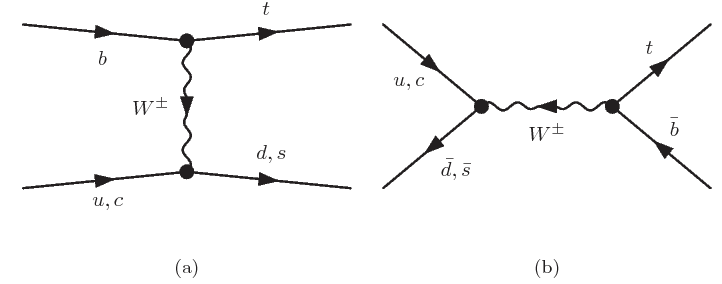
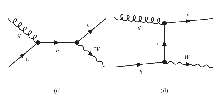
There are three separate modes for single top production. They differ according to the associated particle produced with the top and the initial particles producing the top. These processes can be categorised according to the the virtuality of the $W$ boson. All these processes involve the $Wtb$ coupling; single top production through $t$-channel (which has the largest cross section at the LHC), through $s$-channel and in association with a $W$-boson. The corresponding Feynman diagrams are depicted in Fig. 1.

Figure 1: LO parton level Feynman diagrams of single top production at hadron colliders.

Single top production, although has smaller rate than $t\bar{t}$ production, is phenomenologically very interesting. First, it allows a direct measurement of $V_{tb}$ in the Cabbibo-Kobayashi-Maskawa mixing matrix Alwall:2006bx ; Cao:2015qta . Inference on the $b$-quark density within the proton is possible as well by measuring single top production cross section both through $t$-channel and $Wt$ process. In single top quark production, the produced top is highly polarised allowing for a direct test of the $V-A$ structure of weak interaction Mahlon:1999gz . Finally, single top production is one of the interesting channels to look for new physics beyond the Standard Model Tait:2000sh ; Cao:2007ea ; Cao:2006wk ; Huang:2017yso . Extensive studies of single top production at hadron colliders including radiative corrections have been performed at NLO Campbell:2009ss ; Bordes:1994ki ; Stelzer:1997ns ; Sullivan:2004ie ; Campbell:2004ch ; Campbell:2005bb ; Cao:2004ap ; Cao:2005pq ; Bothmann:2017jfv and NNLO Brucherseifer:2014ama ; Berger:2016oht ; Berger:2017zof in the strong coupling. Furthermore, NLO calculations of single top production matched with parton showers become available within MC@NLO Frixione:2005vw ; Frixione:2008yi and POWHEG Alioli:2009je ; Re:2010bp . Recently, a transverse momentum resummation at NLO+NLL for single top production through $t$-channel has been proposed in Cao:2018ntd . Single top production cross sections have been measured by the ATLAS and CMS collaborations at $\sqrt{s}=7\oplus 8\text{ TeV}$ Aad:2014fwa ; Aad:2015upn ; Aad:2015eto ; Khachatryan:2014iya ; Chatrchyan:2012ep ; Chatrchyan:2011vp ; Chatrchyan:2014tua ; Chatrchyan:2012zca ; Khachatryan:2016ewo and $\sqrt{s}=13\text{ TeV}$ Aaboud:2016lpj ; Aaboud:2016ymp ; Sirunyan:2016cdg . These results were found in agreement with the SM predictions.

The top quark has a very short lifetime, $\tau_{t}\simeq G_{F}^{-1}m_{t}^{-3}\ll m_{t}/\Lambda_{\mathrm{QCD}}^{2}$, which implies that it decays before hadronization effects take place. Hence, all its properties can be studied by looking at the kinematical distributions of its decay products. The top quark decays with almost a $100\%$ branching fraction into $W^{\pm}b$. Furthermore, due to the weak interaction universality, this process has certain pattern, the so-called $V-A$ structure which manifests itself at the lowest order in perturbation theory. Departures from this universal structure are possible through radiative corrections in the SM and/or new physics effects. This departure might be seen as the presence of the so-called anomalous $Wtb$ couplings. One possible parametrization of these couplings is the use of effective field theoretical approach where $SU(3)_{c}\otimes SU(2)_{L}\otimes U(1)_{Y}$ gauge invariant and $6$-dimensional operators are added to the SM Lagrangian Buchmuller:1985jz ; Grzadkowski:2003tf ; Grzadkowski:2010es ; AguilarSaavedra:2008zc . A global fit of these operators to the existing data has been recently done in Durieux:2014xla ; Rosello:2015sck ; Buckley:2015lku ; Buckley:2015nca .

The transition amplitude for top quark decay into a $W$-boson and a $b$-quark can be written as

$$\mathcal{M}(t\to bW^{+})=\frac{-e}{\sqrt{2}\sin\theta_{W}}\bar{u}_{b}(p_{b})\Gamma^{\mu}_{tbW}u_{t}(p_{t})\epsilon_{\mu}^{*}(q),$$ (1)

with

$$\Gamma^{\mu}_{tbW}=-\frac{ig}{\sqrt{2}}\bigg{[}\gamma^{\mu}(V_{L}P_{L}+V_{R}P_{R})+\frac{i}{M_{W}}\sigma^{\mu\nu}q_{\nu}(g_{L}P_{L}+g_{R}P_{R})\bigg{]},$$

where $q=p_{t}-p_{b}$ is the momentum of the $W^{\pm}$ boson (which is assumed to be on-shell) and $P_{L,R}=1/2(1\pm\gamma_{5})$ are the projection operators, $V_{L},V_{R},g_{L}\text{ and }g_{R}$ are called anomalous couplings. In the SM, at tree level, $V_{L}=V_{tb}$ and $V_{R}=g_{L}=g_{R}=0$ whereas EW and QCD radiative corrections induce non-zero values of the anomalous couplings. Computations of the anomalous couplings have been performed in Czarnecki:1990kv ; Li:1990qf ; Bernreuther:2008us ; Drobnak:2010ej ; GonzalezSprinberg:2011kx ; Duarte:2013zfa ; Gonzalez-Sprinberg:2015dea ; Arhrib:2016vts ; Ayala:2016djv ; Martinez:2016fyd both in the SM and certain extensions of it. It was found that SM corrections to anomalous couplings are extremely small, i.e $g_{L}=-(1.247+0.002747i)\times 10^{-3}$, $g_{R}=-(8.6+2.05i)\times 10^{-3}$ and $V_{R}=(2.911+0.9i)\times 10^{-3}$ Arhrib:2016vts . Furthermore, the dominant contribution comes from QCD whereas EW corrections are subleading accounting about $8$–$15\%$ of the total contribution. Contributions of the anomalous $Wtb$ couplings to various flavour observables have been considered in Drobnak:2011wj ; Drobnak:2011aa .

As mentioned above, the top quark produced in association with a quark or $W$, is highly polarised. This polarisation is decided by the anomalous $tbW$ couplings involved in the production of the single top. The production cross-section, the polarisation of the top and the energy distributions of the decay products of the single top, all carry information about these anomalous couplings. In fact, recently a study Godbole:2006tq had shown how one can simultaneously study the top polarisation as well as the $Wtb$ anomalous coupling and constructed some asymmetries in the observables which are sensitive to both. However, it did not make any reference to a specific top production mechanism. It was pointed out in Cao:2015doa that measuring accurately single top production cross sections throught $t$- and $tW$ channels would constrain effectively the anomalous $Wtb$ couplings. In this paper we wish extend the analysis of the observables suggested in Godbole:2006tq as well as the cross-section information, to the single top production via $t$-channel.

Thus the aim of this paper is to make a study of the sensitivity of the LHC to the anomalous coupling $g_{R}$ using energy and angular observables in $t$-channel single top production at $\sqrt{s}=13$ TeV. The observables used in our analysis consist of asymmetries based on energy and angular distributions of the top quark decay products. As we will see in this paper, their use will give additional information about the existence of possible anomalous couplings in the $Wtb$ vertex. Since these observables depend on polarisation, it is expected that they will be robust against QCD radiative corrections. In fact this was demonstrated explicitly in an analysis of the charged Higgs production Godbole:2011vw . In this work also we perform a comparative study at LO and NLO in the strong coupling constant.

We use observables suggested in Prasath:2014mfa , but many of them were proposed long time ago in Godbole:2006tq ; Shelton:2008nq and were used for several studies (see Rindani:2011pk ; Godbole:2011vw ; Belanger:2012tm ; Godbole:2015bda ; Rindani:2015vya ). In addition, we separate the study into two different categories; parton and particle level. In the former case, no cuts are imposed on the particles’ momenta while in the latter loose cuts are imposed. The effects of such kinematical cuts were found to be quite important because these affect the shape of the distributions and hence also the projected limits from the results at the parton level. We stress out that these asymmetries are of extreme importance for future experimental analyses and can be used in several channels that involve the top quark and in different collider machines. We will show, in this paper, that using NLO matrix elements is mandatory for future experimental analyses. In this study, following the limits from $\text{BR}(b\to s\gamma)$, we set $V_{R}=g_{L}=0$ and $g_{R}$ will be taken to be real.

The paper is outlined as follows: In section 2, we review the limits on the anomalous $Wtb$ couplings from direct experimental searches and from statistical fits to several measurements. The setup of the calculation and details about event selection are summarized in section 3. In section 4, we show the computations of single top production through $t$-channel at LO and NLO both in the SM and the SM augmented by anomalous $Wtb$ coupling. The studied observables are briefly discussed in section 5. Numerical results and sensitivity projections are shown in section 6. In section 7, we draw our conclusions. Details about the interpolation procedure are shown in appendix A.

2 Limits on anomalous $Wtb$ couplings

Anomalous $Wtb$ couplings are constrained both indirectly from flavour changing decays such as $b\rightarrow s+\gamma$ as well as from measurements at both the Tevatron and the LHC: those of helicity fractions of the $W$ produced in top decay, both in pair production of the top as well as the single top production, as well as the spin-spin correlations in top pair production etc. A summary of early constraints can be found in Bernreuther:2008ju . Measurement of $b\rightarrow s+\gamma$ branching ratio constrains $V_{R},g_{L}$ strongly, however $g_{R}$ is rather weekly constrained Grzadkowski:2008mf . Measurements of the $W$-boson helicity fraction in top pair production at the Tevatron Abazov:2012uga as well at the LHC Aad:2012ky ; Chatrchyan:2013jna ; Aaboud:2016hsq . In fact an analysis of a combination of the measurements of the BR($b\rightarrow s\gamma$) Grzadkowski:2008mf and the $W$ helicity fractions at the Tevatron Abazov:2012uga together, had shown that $|g_{R}|$ is the only coupling that could have nontrivial values. The large increase of single top production cross-sections with increasing energy, from Tevatron to the LHC, meant that one could also use the single top processes to this end as well Chatrchyan:2013jna ; Khachatryan:2014vma ; Aad:2015yem ; Khachatryan:2016sib ; Aaboud:2017aqp . LHC experiments have used helicity fraction of the $W$ produced in the $t$ decay Aad:2012ky , the double differential decay rate of the singly produced top quark Aad:2015yem , asymmetries constructed out of $W$-boson angular distributions Aaboud:2017aqp as well as the triple differential decay distributions for the $t$ quark Aaboud:2017yqf . In these analyses limits on various anomalous couplings are obtained under different assumptions; sometimes letting all the couplings vary around their SM values or sometimes keeping some of the couplings fixed at their SM values and so on. Furthermore, depending on the variables used, limits can be obtained on the real or imaginary parts of these anomalous couplings. Analyses which tried to constrain all the anomalous couplings simultaneously, using only the data on single top at the LHC Khachatryan:2016sib ; Aaboud:2017yqf with no assumptions on value of $V_{L}$ still allow values of $|g_{R}|\sim 0.1$–$0.2$. Fits assuming $V_{L}=1$ from $t\bar{t}$ production Aaboud:2016hsq by ATLAS also allow large values of $g_{R}(\sim 0.7)$ but these are in conflict with the cross-section measurements of single top processes and hence cannot be taken seriously. On the other hand, a phenomenological analysis of only the collider data, viz. the single top cross-sections and $W$ helicity fractions from both the Tevatron and the LHC Fabbrichesi:2014wva , obtains mildest constraints on $|g_{R}|$ and $V_{R}$.

In addition, a combination of different measurements corresponding to electron and neutron electric dipole moments (EDM), top quark observables and oblique parameters, constrains both the imaginary and real parts of the tensorial couplings $g_{R}$ and $g_{L}$ Cirigliano:2016njn ; Cirigliano:2016nyn . In the end we note that while the imaginary parts of anomalous tensorial couplings are most severely constrained by EDM’s of neutron and electron, BR($b\rightarrow s\gamma$) constrains $|g_{L}|$ and $W$-helicity fraction from the collider data constrain the $|g_{R}|$ most effectively. Recentl global fits to the LHC and Tevatron data Birman:2016jhg ; Castro:2016jjv ; Hioki:2016xtc ; Deliot:2017byp ; Xiong:2018mkc and the limits on $g_{R}$ are not very strong.

A summary of current limits and analyses can be found in Patrignani:2016xqp . For reference, we depict some limits from experimental searches and from BR($b\to s\gamma$) in Table 1. All this discussion thus tells us that it is of great interest to see how the collider data on cross-section and top polarisation in single top production can constrain $g_{R}$. We proceed now to discuss the procedure to do so using new observables.

Constraint	Limits	Reference
BR($b\to s\gamma$)	$-0.15<\text{Re}(g_{R})<0.57,-7\times 10^{-4}\leq V_{R}\leq 2.5\times 10^{-3}$	Grzadkowski:2008mf
	$-1.3\times 10^{-3}\leq g_{L}\leq 4\times 10^{-4}$
$W$ helicity fractions	$\textrm{Re}(V_{R})\in[-0.20,0.23],\textrm{Re}(g_{L})\in[-0.14,0.11],$	Aad:2012ky
	$\textrm{Re}(g_{R})\in[-0.08,0.04].$
	$\text{Re}(g_{R})\in[-0.24,0.20],\text{Re}(g_{L})\in[-0.14,0.10]$	Chatrchyan:2013jna
	$\text{Re}(g_{L})\in[-0.30,0.25],\text{Re}(g_{R})\in[-0.15,0.10]$	Khachatryan:2014vma
double differential cross section	$\text{Re}\left(\frac{g_{R}}{V_{L}}\right)\in[-0.36,0.10]\text{Im}\left(\frac{g_{R}}{V_{L}}\right)\in[-0.17,0.23]$	Aad:2015yem
$t$-channel cross section	$V_{L}>0.98,|V_{R}|<0.16$	Khachatryan:2016sib
	$|g_{L}|<0.057,-0.049<g_{R}<0.048$
$W$-boson polarisation	$V_{R}\in[-0.24,0.31],g_{L}\in[-0.14,0.11],$	Aaboud:2016hsq
	$g_{R}\in[-0.02,0.06]\cup[0.74,0.78]$
	$\text{Im}(g_{R})\in[-0.18,0.06]$	Aaboud:2017aqp
triple differential cross section	$\left|\frac{V_{R}}{V_{L}}\right|<0.37,\left|\frac{g_{L}}{V_{L}}\right|<0.29$	Aaboud:2017yqf
	$\text{Re}\left(\frac{g_{R}}{V_{L}}\right)\in[-0.12,0.17],\text{Im}\left(\frac{g_{R}}{V_{L}}\right)\in[-0.07,0.07]$

Table 1: Summary of the limits on anomalous $Wtb$ couplings from BR($b\to s\gamma$) and from direct experimental searches. A complete listing can be found in the PDG Patrignani:2016xqp .

3 Setup and event selection

For this study, we consider single top production through $t$-channel in $pp$ collisions at $\sqrt{s}=13\text{ TeV}$. For electroweak couplings, we use the $G_{\mu}$-scheme, in which the input parameters are $G_{F},\alpha_{\textrm{em}}(0)\text{ and }M_{Z}$. We choose $G_{F}=1.16639\times 10^{-5}\text{GeV}^{-2}$, $\alpha_{\textrm{em}}^{-1}(0)=137$ and $M_{Z}=91.188\text{ GeV}$. From these input parameters, $M_{W}$ and $\sin^{2}\theta_{W}$ are obtained. Furthermore, the top quark pole mass is chosen to be $m_{t}=173.21\text{ GeV}$. The computation of single top production cross section was done in the $5$FS with massive (massless) $b$-quark at LO (NLO). We use the NNPDF30 PDF sets Ball:2014uwa with the LHAPDF6 interpolator tool Buckley:2014ana with $\alpha_{s}(M_{Z})=0.118$. Throughout this study, we will use fixed factorization and renormalization scales, i.e $\mu_{F}=\mu_{R}=m_{t}$.

Events are generated with Madgraph5$\_$aMC@NLO Alwall:2011uj ; Alwall:2014hca in the SM at Leading Order (LO) and Next-to-Leading Order (NLO) and the SM with anomalous couplings at LO. The right tensorial anomalous coupling $g_{R}$ is implemented by hand in a UFO model file Degrande:2011ua . The model file were validated by comparing some calculations to several results existing in the literature Rindani:2011pk ; Cao:2015doa concerning cross section calculations and several distributions in $t$- and $tW$ channels and we found excellent agreement. The produced events were decayed with MadSpin Artoisenet:2012st which uses the method developed in Frixione:2007zp to keep full spin correlations. The decayed events are passed to PYTHIA8 Sjostrand:2014zea to include parton showers (ISR and FSR) and hadronization. Parton showering algorithm is based on dipole type $p_{\perp}$ evolution Sjostrand:2004ef . The other parameters are set according to the Monash tune Skands:2014pea . We have adopted the MC@NLO scheme Frixione:2002ik for consistent matching of hard-scattering matrix elements and parton shower MC. RIVET Buckley:2010ar was used for analysis of the events. For jet clustering, we use FastJet Cacciari:2011ma with an anti-$k_{\perp}$ algorithm and jet radius $R=0.4$ Cacciari:2008gp .

We, first, perform a partonic level analysis (no showers, no soft QCD effects and no cuts on the kinematical quantities). We then, perform a particle level analysis (without detector effects) of the showered events. Throughout this paper, we will show results at both the partonic and the particle levels. For the particle level analysis, we require a topology consisting of exactly one isolated charged lepton (electron or muon), missing energy $E_{\text{T}}^{\text{miss}}$ and at least two jets with at least one of them is $b$-tagged. First, we require exactly one isolated charged lepton with transverse momentum $p_{\perp}(\text{lepton})>10\text{ GeV}$ and pseudorapidity $|\eta|<2.5$. We require at least two jets where one of them is tagged with $|\eta|<2.5$ and $p_{\perp}(\text{jet})\geq 25\text{ GeV}$. Further isolation requirements are applied to jets, i.e the angular separation should be always $\Delta R=\sqrt{\Delta\eta^{2}+\Delta\phi^{2}}>0.5$ for any two jets in the event and $\Delta R(\text{jet},\text{lepton})>0.4$.

4 Single top production through $t$-channel

In this section, we discuss single top production cross section in the SM at LO and NLO. We illustrate at the end of the section the method that we used to include anomalous $Wtb$ coupling in the production at NLO.

4.1 LO calculation in the SM

At LO, there are two generic contributions to the $t$-channel process. The first contribution corresponds to the subprocess:

$$b\hskip 5.69046ptq\to t\hskip 5.69046ptq^{\prime},$$ (2)

and the second contribution represents the subprocess:

$$b\hskip 5.69046pt\bar{q}^{\prime}\to t\hskip 5.69046pt\bar{q},$$ (3)

where $q=u,c$ and $q^{\prime}=d,s$. Furthermore, contributions to the $t$-channel process involving the negligble elements of the Cabbibo-Kobayashi-Maskawa (CKM) mixing matrix such as $V_{td}\text{ and }V_{ts}$ were not taken into account. We have computed the inclusive LO cross sections at $\sqrt{s}=13$ TeV. Due to the dominance of the valence u-quark PDF over the sea anti-quarks, the subprocess 2 gives the dominant contribution which accounts of about $77\%$ of the total cross section.

4.2 The $t$-channel at NLO in the SM

Figure 2: Feynman diagrams contributing to $bq\to tq^{\prime}$ subprocess at NLO in the SM where $q=u,c$ and $q^{\prime}=d,s$.

Figure 3: Feynman diagrams contributing to $b\bar{q}^{\prime}\to t\bar{q}$ subprocess at NLO in the SM where $q=u,c$ and $q^{\prime}=d,s$.

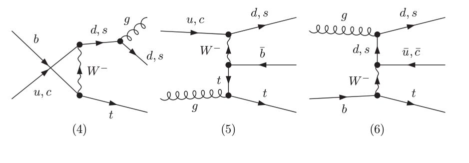
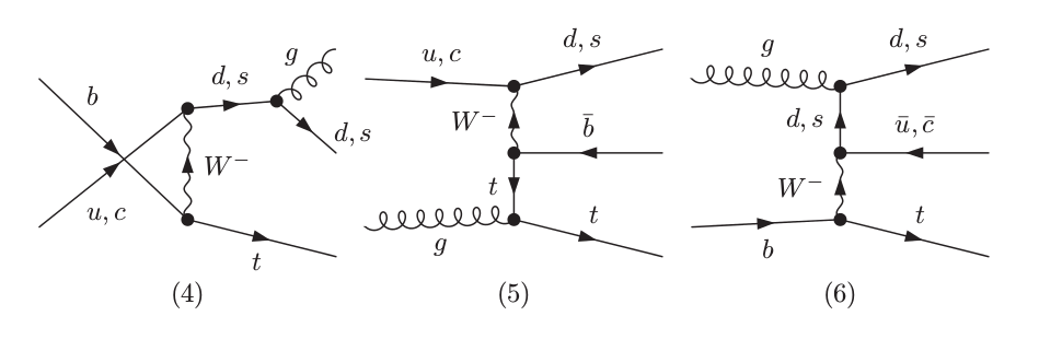
Further contributions to the $t$-channel process, at NLO exist. Such contributions include virtual one-loop corrections to the tree level process as well as tree level $2\to 3$ real emission processes where the additional emitted parton is soft or collinear. Parton level Feynman diagrams are depicted in figures 2 and 3. All the possible flavours that might contribute to this process were included. Due to color conservation, box diagrams do not contribute to the cross section at NLO.

Order	$\sigma$ [pb]	$\delta\sigma_{\mu}$ [%]	$\delta\sigma_{\textrm{PDF}}$ [%]
LO	$128.67$	${}^{+9.12}_{-11.3}$	$\pm 8.88$
	$50.50$	${}^{+10.4}_{-12.5}$	$\pm 9.65$
NLO	$141.8$	${}^{+2.8}_{-2.5}$	$\pm 1.2$
	$75.11$	${}^{+2.8}_{-2.9}$	$\pm 1.1$

Table 2: $t$-channel production cross section at LO and NLO at $\sqrt{s}=13$ TeV. Uncertainties due to scale variations and PDF are shown. First rows show the values of the cross section without cuts and in the second rows the cross sections are computed using the cuts highlighted in section 3.

We have computed the total cross section at $\sqrt{s}=13\text{ TeV}$ with $\mu_{R}=\mu_{F}=m_{t}$. The dominance of the valence $u$-quark PDF implies that the cross section from the contribution of Feynman diagrams in Fig. 2 is dominant. We have also estimated theoretical uncertainties on the inclusive cross section both at LO and NLO from scale variations and from PDF. Theoretical uncertainties which are due to scale variations are estimated by varying simultaneously the hard factorization and renormalization scales around their nominal values, i.e :

$$0.5\leq\mu_{R}/\mu_{R,0},\mu_{F}/\mu_{F,0}\leq 2,$$ (4)

where $\mu_{R,0}$ ($\mu_{F,0}$) is the central renormalization (factorization) scale. Thus, obtaining an envelope of the nine possible variations. PDF uncertainties are obtained using the replicas method where each PDF set has one central and 50 members corresponding to the minimal fit and the eigenvectors respectively. The results for the inclusive cross section at LO and NLO along with their theoretical uncertainties are depicted in Table 2. After cuts were imposed, the total rate decreases by a factor of $\simeq 2.5$ and $\simeq 1.9$ at LO and NLO respectively. Furthermore, theoretical uncertainties due to scale variations increase in both LO as well as NLO with the former has even larger relative increase than the latter. The most important consequence of imposing cuts on the decay products is that the $K$-factor of the fiducial cross section increase to about $1.5$ while the theoretical uncertainties at LO do not change much. An immediate consequence of such observation is that the fiducial cross section at NLO is outside the allowed range of scale variations’ uncertainty at LO since $\sigma_{\textrm{LO}}^{\textrm{max}}=50.5+\delta\sigma_{\mu}^{+}\oplus\delta\sigma_{\textrm{PDF}}^{+}\approx 58$ pb $<\sigma_{\textrm{NLO}}$. Hence, for any future analysis or fit involving the cross section of single top through $t$-channel, at least the calculation at NLO should be used.

4.3 Including anomalous $Wtb$ couplings

The presence of anomalous $Wtb$ couplings modifies single top quark production cross sections. The production cross section of a top quark through $t$-channel in $pp$ collisions can be expressed as function of anomalous right tensorial coupling $g_{R}$ as

$$\sigma_{\text{t-ch}}=\sigma_{\text{t-ch}}^{\text{SM}}\bigg{(}1+\kappa_{1}g_{R}+\kappa_{2}|g_{R}|^{2}\bigg{)},$$ (5)

where $\kappa_{1,2}\equiv\kappa_{1,2}(m_{t},m_{b},M_{W},\sqrt{s})$. They are determined from a fit and are given by

$$\kappa_{1}=0.45485\quad(0.66433)\qquad\textrm{without cuts (with cuts)},$$

$$\kappa_{2}=2.05348\quad(3.21011)\qquad\textrm{without cuts (with cuts)},$$

at $\sqrt{s}=13$ TeV. In eqn. 5, $\sigma_{\text{t-ch}}^{\text{SM}}$ is the SM cross section at LO (see e.g. Table 2). We can see that imposing cuts strengthen the dependence of the cross section on the anomalous coupling by a factor of $\simeq 1.5$. Although the quadratic term is about 5 times larger than the linear one its contribution to the cross section is mild even for the extreme values of $g_{R}$, i.e $g_{R}=\pm 0.2$. The results we obtained were compared with those presented in Cao:2015doa and we found excellent agreement.

Taking into account the anomalous $Wtb$ coupling in the production at NLO is not straightforward. The reason is that one cannot renormalize high dimensional operators using the traditional on-shell renormalization schemes. Using alternative schemes for the renormalization of the SM wave functions and parameters will result in large theoretical uncertainties. However, including anomalous $Wtb$ couplings in the production is very interesting since they completely change the chiral structure of the $Wtb$ vertex and hence the top quark polarisation which in fact improve the sensitivity of most the observables on the anomalous couplings. We include their effects as a shift on the production while neglecting interference between the virtual corrections and tree level amplitudes with anomalous couplings. Hence, three samples will be generated with the first one corresponds to SM amplitude at NLO, the second to the LO amplitude in the SM and the third one to the amplitude with anomalous couplings at tree level. The transition amplitude for the process

$$pp\to t+X\to b\ell^{+}\nu_{\ell}+X,$$

can be written as

$$\mathcal{M}(\lambda)=\mathcal{P}(\lambda)\mathcal{D}(\lambda),$$ (6)

where $\mathcal{P}$ ($\mathcal{D}$) is the production (decay) matrix elements for the top quark.

For convenience ($\lambda$) and ($\lambda^{\prime}$) stand for the helicity labelling of all particles. The pure SM tree level amplitude (equivalent to $g_{R}=0$) is $\mathcal{P}_{0}^{\text{SM}}$. The contribution of the anomalous coupling $g_{R}$ will only be taken into account at tree- level and will be denoted $\mathcal{P}_{0}^{g_{R}}$. The full tree-level amplitude, anomalous amplitude, will be denoted $\mathcal{P}_{0}^{\text{ano.}}$, such that

$$\mathcal{P}_{0}^{\text{ano.}}=\mathcal{P}_{0}^{\text{SM}}+\mathcal{P}_{0}^{g_{R}}$$ (7)

Since the radiative corrections at the level of the decay are very small in the SM (see e.g. Gao:2012ja ), the decay part will be considered at tree-level only. For the production part, at tree-level, with the inclusion of the anomalous part we have

$$\mathcal{P}_{\textrm{tree}}(\lambda,\lambda^{\prime}) = \mathcal{P}_{\textrm{LO}}(\lambda,\lambda^{\prime})=(\mathcal{P}_{0}^{\text{SM}}(\lambda)+\mathcal{P}_{0}^{g_{R}}(\lambda^{\prime}))(\mathcal{P}_{0}^{\text{SM}}(\lambda)+\mathcal{P}_{0}^{g_{R}}(\lambda^{\prime}))^{*}$$ (8)

$$\equiv \mathcal{P}_{0}^{\text{ano.}}(\lambda)\mathcal{P}_{0}^{\text{ano.}}(\lambda^{\prime})^{*}.$$

The one-loop radiative corrections will only apply to the SM part. The first higher order contribution consists of the one-loop $2\to 2$ virtual correction that includes also counterterms, $\delta\mathcal{P}_{V}(\lambda)$. To this one needs to add the pure SM radiative, $2\to 3$ emission. First of all, for the $2\to 2$ one-loop virtual correction and the $g_{R}$ contribution we may write

$$\mathcal{P}_{1}(\lambda,\lambda^{\prime}) = (\mathcal{P}_{0}^{\text{SM}}(\lambda)+\delta\mathcal{P}_{V}(\lambda)+\mathcal{P}_{0}^{g_{R}}(\lambda^{\prime}))(\mathcal{P}_{0}^{\text{SM}}(\lambda)+\delta\mathcal{P}_{V}(\lambda)+\mathcal{P}_{0}^{g_{R}}(\lambda^{\prime}))^{*}$$ (9)

$$\simeq \mathcal{P}_{V}(\lambda,\lambda^{\prime})+\mathcal{P}_{0}^{\text{ano.}}(\lambda)\mathcal{P}_{0}^{\text{ano.}}(\lambda^{\prime})^{*}-\mathcal{P}_{0}^{\text{SM}}(\lambda)\mathcal{P}_{0}^{\text{SM}}(\lambda^{\prime})^{*},$$

where

$$\mathcal{P}_{V}(\lambda,\lambda^{\prime})=\mathcal{P}_{0}^{\text{SM}}(\lambda)\mathcal{P}_{0}^{\text{SM}}(\lambda^{\prime})^{*}+\mathcal{P}_{0}^{\text{SM}}(\lambda)\delta\mathcal{P}_{V}(\lambda^{\prime})^{*}+\delta\mathcal{P}_{V}(\lambda)\mathcal{P}_{0}^{\text{SM}}(\lambda^{\prime})^{*}$$ (10)

Including and integrating over real emission, $\mathcal{P}_{R}^{\text{SM}}(\lambda)$, and adding it to the virtual correction $\mathcal{P}_{V}(\lambda,\lambda^{\prime})$ of Eq. 10 will give the full NLO SM result. What we will refer to as the full NLO (including the LO anomalous part) is

$$\mathcal{P}_{\text{NLO}}(\lambda,\lambda^{\prime})=\underbrace{\mathcal{P}_{V}(\lambda,\lambda^{\prime})+\mathcal{P}_{R}^{\text{SM}}(\lambda,\lambda^{\prime})}_{\text{sample 1}}+\underbrace{\mathcal{P}_{0}^{\text{ano.}}(\lambda)\mathcal{P}_{0}^{\text{ano.}}(\lambda^{\prime})^{*}}_{\text{sample 2}}-\underbrace{\mathcal{P}_{0}^{\text{SM}}(\lambda)\mathcal{P}_{0}^{\text{SM}}(\lambda^{\prime})^{*}}_{\text{sample 3}}.$$ (11)

In order to reproduce the data including both the NLO SM and the anomalous contribution (with its quadratic part) we therefore, for the same phase space point, generate three samples. One for the full anomalous part at tree-level, one for the SM tree-level part (which has to be subtracted to avoid double counting) and one for the SM NLO (which includes the SM tree, virtual and real emission).

5 Observables

In this section, we review the observables that we will be using for our analysis of anomalous $Wtb$ couplings. They consist of asymmetries constructed from the energy and angular distributions of the top quark decay products in single top production through $t$-channel.

We define an asymmetry with respect to a kinematical variable $\mathcal{O}$ by:

$$A_{\mathcal{O}}=\frac{\int_{\mathcal{O}_{\text{min}}}^{\mathcal{O}_{\text{R}}}\frac{d\sigma}{d\mathcal{O}}d\mathcal{O}-\int_{\mathcal{O}_{\text{R}}}^{\mathcal{O}_{\text{max}}}\frac{d\sigma}{d\mathcal{O}}d\mathcal{O}}{\int_{\mathcal{O}_{\text{min}}}^{\mathcal{O}_{\text{R}}}\frac{d\sigma}{d\mathcal{O}}d\mathcal{O}+\int_{\mathcal{O}_{\text{R}}}^{\mathcal{O}_{\text{max}}}\frac{d\sigma}{d\mathcal{O}}d\mathcal{O}},$$ (12)

where $\frac{d\sigma}{d\mathcal{O}}=\frac{d\sigma(pp\to tX\to\ell^{+}\nu_{\ell}bX)}{d\mathcal{O}}$, $\ell=e,\mu$, is the differential cross section of the top quark with respect to the variable $\mathcal{O}$ and $\mathcal{O}_{R}$ is a reference point around which the asymmetry will be evaluated. $\mathcal{O}_{R}$ will be chosen such that the evaluated asymmetry is sensitive to the anomalous coupling and allows for a comparison of cases of different values of the parameter. In what follows, kinematical quantities written with a superscript "0" are given in the top quark’s rest frame. Otherwise, they are given in the laboratory frame.

5.1 Lepton polar asymmetry

Figure 4: $\cos\theta_{\ell}$ distribution in the top quark rest frame using full partonic information (left) and with the cuts implemented at the particle level (right) at NLO.

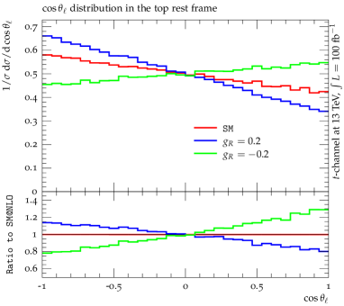
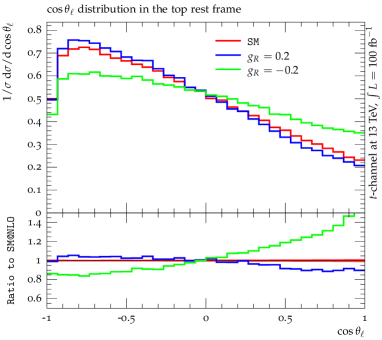
The polar angle of the charged lepton, denoted by $\theta_{\ell}^{0}$, is defined by

$$\cos\theta_{\ell}^{0}=\frac{\textbf{p}_{\ell}\cdot\textbf{p}_{t}}{|\textbf{p}_{\ell}||\textbf{p}_{t}|},$$ (13)

with $\textbf{p}_{\ell}$ is the three-momentum of the charged lepton in the top quark rest frame and $\textbf{p}_{t}$ is the top quark three-momentum in the laboratory frame. This observable is a good probe of the top quark polarisation. However, given that the presence of anomalous coupling changes the chiral structure of the top quark, we expect that it is a good probe of the anomalous coupling too. This can clearly be seen in Fig. 4 where the $\cos\theta_{\ell}^{0}$ distribution is plotted in both the SM and for $g_{R}=\pm 0.2$. We can see that the effect of the anomalous coupling on the $\cos\theta_{\ell}^{0}$ is important and which can even change the slope of the distribution for $g_{R}=-0.2$. Although the presence of cuts (right panel of Fig. 4) modifies the sensitivity of this observable, it can be used for searches of the anomalous couplings. However, the measurement of the polar distribution is quite challenging since it requires a full reconstruction of the top quark momentum. This is hard to be achieved due to the presence of missing energy in the semi-leptonic decay of the top quark. Nevertheless, several measurements of the charged lepton angle in the helicity basis exist, e.g. in the $t\bar{t}$ system Aaboud:2016bit . Hence, it can possibly be measured in the $t$-channel process in the future. From Fig. 4, we define the reference point for the $A_{\theta_{\ell}^{0}}$ to be $\cos\theta_{\ell}^{0}=0$.

5.2 Charged lepton Energy

In addition to the angular polar distribution in the top quark’s rest frame, two other observables constructed from the charged lepton energy are considered here. We define a dimensionless variable, $x_{\ell}$, by:

$$x_{\ell}=\frac{2E_{\ell}}{m_{t}},$$ (14)

where $E_{\ell}$ is the lepton’s energy in a given frame and $m_{t}$ is the top quark mass. We consider the energy of the charged lepton in two different frames; the top quark’s rest frame and the $pp$ center-of-mass frame.

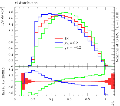
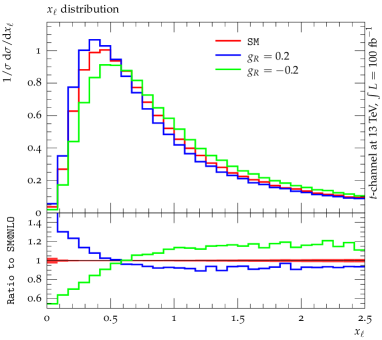
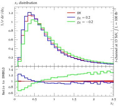
It was shown that, in the top quark’s rest frame, this asymmetry is a pure probe of the anomalous $Wtb$ coupling regardless the top quark production mechanism (or in other words top quark polarisation) Prasath:2014mfa . Hence, at the experimental level, full advantage of this observable should be taken by measuring it in several channels. However, for its measurement, a reconstruction of the top quark momentum is needed. We depict the $x_{\ell}^{0}$ in the SM and for $g_{R}=\pm 0.2$ in Fig. 5. The reference point for the corresponding asymmetry, $A_{x_{\ell}^{0}}$ is chosen to be $x_{\ell^{0},c}=0.5$, i.e the value $x_{\ell}^{0}$ at the peak position in the SM Godbole:2015bda .

Figure 5: $x_{\ell}$ distribution in the top quark rest frame using full partonic information (left) and with the cuts implemented at the particle level (right) at NLO.

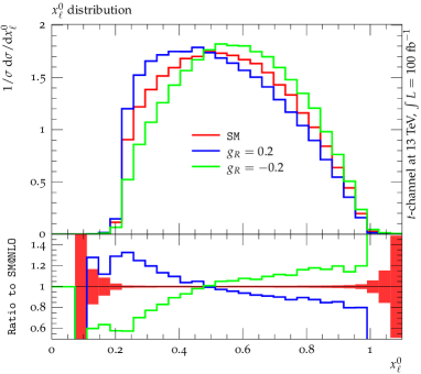
The situation is different for $x_{\ell}$ in the laboratory frame which is shown in Fig. 6. This observable is sensitive to both the anomalous coupling as well as the top polarisation and has a high sensitivity to the anomalous coupling for small values of $x_{\ell}$ for positive values of $g_{R}$ and in the full range of $x_{\ell}$ for negative values of $g_{R}$. However, this observable has a lower sensitivity on the anomalous coupling than $x_{\ell}^{0}$ due to some cancellations which occur between anomalous couplings and other kinematical factors Prasath:2014mfa . Finally, no reconstruction of the top quark momentum is needed in order to measure this observable. A reference point of $x_{\ell,c}=0.6$ is chosen for the evaluation of the corresponding asymmetry Godbole:2015bda .

Figure 6: $x_{\ell}$ distribution in the laboratory frame using full partonic information (left) and with the cuts implemented at the particle level (right) at NLO.

5.3 $u$- and $z$-variables

Figure 7: $u$ distribution in the laboratory frame using full partonic information (left) and with the cuts implemented at the particle level (right) at NLO.

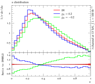
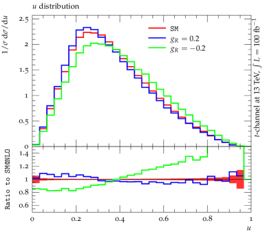
The last two variables from which two different asymmetries will be evaluated have been proposed in Shelton:2008nq as a probe of top quark polarisation for highly boosted top quarks. First, a variable $u$ which measures the energy ratio of the charged lepton to the total visible energy (of the top quark decay). This variable is defined by :

$$u=\frac{E_{\ell}}{E_{\ell}+E_{b}},$$ (15)

where $E_{\ell}$ and $E_{b}$ are the lepton and b-quark ($b$-jet) energies in the laboratory frame. It was found that the $u$-variable is sensitive to both the top quark polarisation and the anomalous $Wtb$ coupling Prasath:2014mfa . We found that including the anomalous $Wtb$ in the production improves the sensitivity of the $u$-variable on $g_{R}$. From experimental point of view, it is possible to measure this variable from a simultaneous measurements of the both the charged lepton and $b$-jet energies in the laboratory frame. This implies that there is no need for reconstructing the top quark momentum. We depict the $u$ variable for three different models at NLO in Fig. 7. From this figure, we choose the reference point $u_{c}=0.4$ which is the intersection point of the three different curves corresponding to the SM and to $g_{R}=\pm 0.2$.

Finally, the $z$ variable, which measures the fraction of the top quark energy taken by the $b$-jet in the laboratory frame, is defined by:

$$z=\frac{E_{b}}{E_{t}},$$ (16)

where $E_{b}$ and $E_{t}$ are the energies of the bottom and top quarks respectively in the laboratory frame. In Fig. 8, we depict the $z$-variable for the SM and $g_{R}=\pm 0.2$. We can see that $z$-variable has a lower sensitivity on the anomalous coupling. Furthermore, its measurement requires a determination of the top quark energy, which by itself depends on the decay mode. The hadronic mode, although has a larger background is better for the measurement of the $z$-variable. The reference point will be chosen to be $z_{c}=0.4$.

Figure 8: $z$ distribution in the laboratory frame using full partonic information (left) and with the cuts implemented at the particle level (right) at NLO.

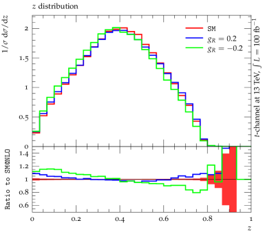
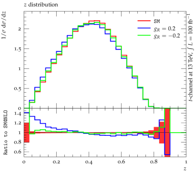
	LO	NLO	NLO/LO
$A_{\theta_{\ell}^{0}}$	$0.110^{+0.0000(+0.0\%)}_{-0.01630(-14.5\%)}$	$0.104^{+0.0000(+0.0\%)}_{-0.0155(-14.9\%)}$	$0.94$
	$0.347^{+0.0000(+0.0\%)}_{-0.0019(-0.5\%)}$	$0.297^{+0.0045(+1.5\%)}_{-0.0023(-0.7\%)}$	$0.85$
$A_{x_{\ell}^{0}}$	$-0.139^{+0.0175(+12.5\%)}_{-0.0000(-0.0\%)}$	$-0.139^{+0.0010(+0.7\%)}_{-0.0000(-0.0\%)}$	$1.0$
	$-0.178^{+0.0000(+0.0\%)}_{-0.0181(-10.2\%)}$	$-0.178^{+0.0025(+1.4\%)}_{-0.0000(-0.0\%)}$	$1.0$
$A_{x_{\ell}}$	$-0.117^{+0.0194(+16.5\%)}_{-0.0000(-0.0\%)}$	$-0.091^{+0.0000(+0.0\%)}_{-0.0063(-6.9\%)}$	$1.3$
	$-0.089^{+0.0000(+0.0\%)}_{-0.0117(-13.1\%)}$	$-0.119^{+0.0073(+6.1\%)}_{-0.0039(-3.2\%)}$	$1.3$
$A_{u}$	$0.133^{+0.0000(+0.0\%)}_{-0.0019(-1.4\%)}$	$0.131^{+0.0000(+0.0\%)}_{-0.0130(-9.9\%)}$	$1.0$
	$0.271^{+0.0106(+3.9\%)}_{-0.0000(-0.0\%)}$	$0.242^{+0.0019(+0.7\%)}_{-0.0038(-1.5\%)}$	$0.9$
$A_{z}$	$-0.090^{+0.0120(+13.3\%)}_{-0.0000(-0.0\%)}$	$-0.074^{+0.0000(+0.0\%)}_{-0.0024(-3.0\%)}$	$0.8$
	$-0.013^{+0.0000(+0.0\%)}_{-0.0074(-56.9\%)}$	$-0.010^{+0.0085(+85\%)}_{-0.0000(-0.0\%)}$	$0.8$

Table 3: Asymmetries and their theoretical uncertainties in the SM at LO and NLO. The first rows for each asymmetry show the partonic level results while the second rows the particle level ones.

6 Results

From the different kinematical distributions shown in section 5, asymmetries are constructed (for more details, see section A). These asymmetries present, except $A_{z}$, a high sensitivity on the anomalous right tensorial coupling as it is depicted in Fig. 9 which is weakened at the particle level. We can see that there are some differences between the central values of the asymmetries at LO and NLO of about $6\%$–$30\%$ depending on the particular asymmetry. However, one notices that these differences are within the theoretical uncertainties which are depicted in Table 3 where only the effect of scale variations is shown. The effect of radiative corrections on the asymmetries depends on the particular variable. At the parton level, two asymmetries are perfectly stable against radiative corrections; i.e $A_{x_{\ell}^{0}}$ and $A_{u}$ while the others can receive corrections of $6\%$ for $A_{\theta_{\ell}^{0}}$, $20\%$ for $A_{z}$ and $30\%$ for $A_{x_{\ell}}$. On the other hand, the theoretical uncertainties due to scale variations are quite large except for $A_{u}$ both at LO and NLO and for $A_{x_{\ell}^{0}}$ at NLO. At the particle level, the corrections to the asymmetries are lower than to the cross sections with again a strong stability against NLO corrections for $A_{x_{\ell}^{0}}$ and $A_{u}$. The theoretical uncertainties due to scale variations are lower than in the parton level case with one notable exception, i.e $A_{z}$ which has very large theoretical uncertainties (see Table 3).

Figure 9: Dependence of different asymmetries as function of the anomalous coupling at the parton level without cuts (left panel) and at the particle level with cuts (right panel). The solid (dashed) lines show the dependence at LO (NLO).

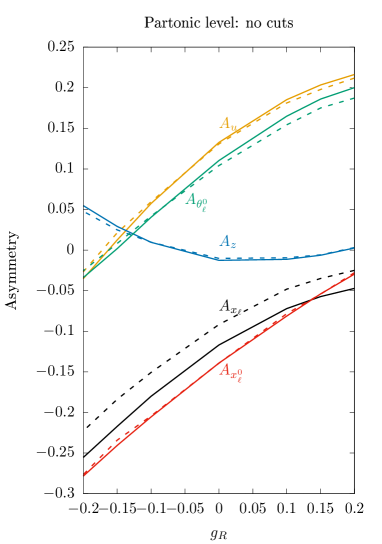
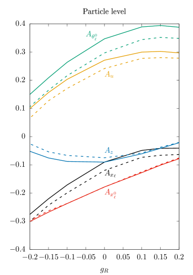
We perform a $\chi^{2}$ exclusion to obtain the limits on the anomalous coupling $g_{R}$. A $\chi^{2}$ is defined as follows

$$\chi^{2}=\sum_{\mathcal{O}}\frac{(A_{\mathcal{O}}-A_{\mathcal{O};\textrm{SM}})^{2}}{\Delta_{\mathcal{O}}^{2}},$$ (17)

where $\mathcal{O}=x_{\ell},x_{\ell}^{0},\cos\theta_{\ell}^{0},z\text{ and }u$. $\Delta_{\mathcal{O}}$ is the sum, by quadrature, of the statistical and theoretical uncertainties on the asymmetry $A_{\mathcal{O}}$ in the SM. The former are defined as

$$\Delta_{\mathcal{O}}^{\mathrm{stat.}}=\frac{\sqrt{1-A_{\mathcal{O}}^{2}}}{\sqrt{N}}.$$ (18)

where $N$ is the number of events

$$N=\sigma_{t}\mathrm{BR}(t\to b\ell\nu_{\ell})\mathcal{L},$$

we assume a luminosity of $\mathcal{L}=100$ fb^-1. Values of $g_{R}$ are excluded within $1\sigma,2\sigma\text{ and }3\sigma$ if the corresponding $\chi^{2}$ is larger than $2.3,5.99$ and $11.8$ respectively. We show in Table 4, individual limits obtained from the different asymmetries at $1\sigma$ both at LO and NLO. We can see that all the asymmetries but $A_{z}$ give strong constraints on the anomalous coupling. Furthermore, the limits placed on the anomalous coupling from $A_{x_{\ell}}$ and $A_{\theta_{\ell}^{0}}$ are strenghten, at the particle level, by about a factor of $2$ and $7$ respectively. This is due to the large theoretical uncertainties on those observables at the partonic level which are significantly reduced when showers and cuts are implemented. Overall, constraints on the anomalous right tensorial coupling are stronger at NLO due to the reduction of theoretical and statistical uncertainties. Before discussing the combination of different asymmetries and its effect on the anomalous coupling, we comment about the experimental uncertainties. Generally, measurement of the asymmetries $A_{x_{\ell}^{0}}$ and $A_{\theta_{\ell}^{0}}$ introduces additional systematic uncertainties since they involve the reconstruction of the top quark rest frame which is very hard for single top production. Hence, although the $A_{x_{\ell}^{0}}$ asymmertry is resilient to NLO corrections, it might not be very efficient in the determination of the anomalous coupling. On the other hand, among all the laboratory frame asymmetries, $A_{u}$ is the most sensitive and involving less systematics (both theoretical and experimental) uncertainties. Combining two asymmetries at one time improves significantly the limits on $g_{R}$. We found that combining $A_{x_{\ell}^{0}}$ and $A_{u}$ gives $[-0.0048,0.0048]$ ($[-0.0021,0.0021]$) at LO (NLO) at the parton level at $1\sigma$. While at the particle level, those limits are weakened to give $[-0.0261,0.0312]$ ($[-0.0052,0.0053]$) at LO (NLO).

These limits can be improved by combining more than one asymmetry at a time. As an example, we estimate projected limits using ten different combinations of the three different asymmetrie. We can see in Tables 5-6 that the limits are improved by about one order of magnitude from those obtained using one asymmetry at a time. In Table 5, we show these limits at the partonic level. We can see that, at LO that six different combinations of the three asymmetries give $g_{R}\in[-0.0103,0.0107]$ at $3\sigma$. The situation is different for the NLO case, where the limits are improved by a factor of $2$ from the combinations $(A_{u},A_{x_{\ell}},A_{x_{\ell}^{0}})$ and $(A_{u},A_{x_{\ell}^{0}},A_{\theta_{\ell}^{0}})$ yielding $g_{R}$ in the interval $[-0.0047,0.0048]$. On the other hand, including showers and cuts do not change much the limits that we obtain but only the combination of the asymmetries change. In Table 6, we can see that six asymmetries give the strongest limit at LO; i.e $g_{R}\in[-0.0112,0.0121]$. While at NLO, we obtain $g_{R}\in[-0.0099,0.0104]$ using the $(A_{u},A_{x_{\ell}^{0}},A_{\theta_{\ell}^{0}})$ combination. However, as this combination involves the $A_{\theta_{\ell}^{0}}$ asymmetry which requires full reconstruction of the top quark direction of motion. Hence, that either the $(A_{u},A_{x_{\ell}},A_{z})$ or $(A_{u},A_{x_{\ell}},A_{x_{\ell}^{0}})$ will do a better job in pinning down the anomalous coupling even the obtained limits are milder than $(A_{u},A_{x_{\ell}^{0}},A_{\theta_{\ell}^{0}})$.

Asymmetry	LO	NLO
$A_{\theta_{\ell}^{0}}$	$[-0.0380,0.0440]$	$[-0.0480,0.0541]$
	$[-0.0052,0.0053]$	$[-0.0082,0.0086]$
$A_{x_{\ell}^{0}}$	$[-0.0417,0.0446]$	$[-0.0026,0.0026]$
	$[-0.0486,0.0542]$	$[-0.0069,0.0070]$
$A_{x_{\ell}}$	$[-0.0500,0.0605]$	$[-0.0193,0.0204]$
	$[-0.0261,0.0321]$	$[-0.0122,0.0131]$
$A_{u}$	$[-0.0046,0.0047]$	$[-0.0036,0.0036]$
	$[-0.0302,0.0402]$	$[-0.0080,0.0085]$
$A_{z}$	$[-0.0702,0.1912]$	$[-0.0738,0.1987]$
	$[-0.1756,0.0876]$	$[-0.0702,0.0490]$

-

Table 4: Individual expected limits at $1\sigma$ on the anomalous coupling $g_{R}$ at LO and NLO using full partonic information (first rows) and at the particle level (second rows).

Combination	$1\sigma$	$2\sigma$	$3\sigma$
$(A_{u},A_{z},A_{x_{\ell}})$	$[-0.0046,0.0047]$	$[-0.0074,0.0076]$	$[-0.0103,0.0107]$
	$[-0.0035,0.0036]$	$[-0.0057,0.0058]$	$[-0.0079,0.0082]$
$(A_{u},A_{x_{\ell}},A_{x_{\ell}^{0}})$	$[-0.0046,0.0046]$	$[-0.0074,0.0076]$	$[-0.0103,0.0107]$
	$[-0.0021,0.0021]$	$[-0.0034,0.0034]$	$[-0.0047,0.0048]$
$(A_{x_{\ell}},A_{x_{\ell}^{0}},A_{\theta_{\ell}^{0}})$	$[-0.0250,0.0266]$	$[-0.0397,0.0438]$	$[-0.0547,0.0629]$
	$[-0.0026,0.0026]$	$[-0.0042,0.0042]$	$[-0.0058,0.0059]$
$(A_{u},A_{z},A_{\theta_{\ell}^{0}})$	$[-0.0046,0.0046]$	$[-0.0074,0.0076]$	$[-0.0103,0.0107]$
	$[-0.0036,0.0036]$	$[-0.0058,0.0059]$	$[-0.0080,0.0083]$
$(A_{u},A_{z},A_{x_{\ell}^{0}})$	$[-0.0046,0.0046]$	$[-0.0074,0.0076]$	$[-0.0103,0.0107]$
	$[-0.0021,0.0021]$	$[-0.0034,0.0034]$	$[-0.0048,0.0048]$
$(A_{u},A_{x_{\ell}},A_{\theta_{\ell}^{0}})$	$[-0.0046,0.0047]$	$[-0.0074,0.0076]$	$[-0.0103,0.0107]$
	$[-0.0035,0.0036]$	$[-0.0056,0.0058]$	$[-0.0079,0.0082]$
$(A_{u},A_{x_{\ell}^{0}},A_{\theta_{\ell}^{0}})$	$[-0.0046,0.0046]$	$[-0.0074,0.0076]$	$[-0.0103,0.0107]$
	$[-0.0021,0.0021]$	$[-0.0034,0.0034]$	$[-0.0047,0.0048]$
$(A_{z},A_{x_{\ell}},A_{\theta_{\ell}^{0}})$	$[-0.0294,0.0335]$	$[-0.0458,0.0562]$	$[-0.0622,0.0822]$
	$[-0.0178,0.0189]$	$[-0.0283,0.0312]$	$[-0.0393,0.0449]$
$(A_{z},A_{x_{\ell}^{0}},A_{\theta_{\ell}^{0}})$	$[-0.0274,0.0299]$	$[-0.0430,0.0496]$	$[-0.0588,0.0713]$
	$[-0.0026,0.0026]$	$[-0.0042,0.0042]$	$[-0.0059,0.0059]$
$(A_{z},A_{x_{\ell}},A_{x_{\ell}^{0}})$	$[-0.0309,0.0348]$	$[-0.0482,0.0581]$	$[-0.0654,0.0840]$
	$[-0.0026,0.0026]$	$[-0.0042,0.0042]$	$[-0.0059,0.0059]$

Table 5: Limits on the anomalous coupling $g_{R}$ at $1\sigma$, $2\sigma$ and $3\sigma$ at the partonic level without cuts. The first row for each combination represents the interval at LO while the second row represents the NLO exclusion.

Combination	$1\sigma$	$2\sigma$	$3\sigma$
$(A_{u},A_{z},A_{x_{\ell}})$	$[-0.0202,0.0233]$	$[-0.0314,0.0403]$	$[-0.0426,0.0616]$
	$[-0.0067,0.0070]$	$[-0.0108,0.0115]$	$[-0.0149,0.0164]$
$(A_{u},A_{x_{\ell}},A_{x_{\ell}^{0}})$	$[-0.0189,0.0215]$	$[-0.0294,0.0368]$	$[-0.0410,0.0555]$
	$[-0.0048,0.0049]$	$[-0.0078,0.0080]$	$[-0.0108,0.0113]$
$(A_{x_{\ell}},A_{x_{\ell}^{0}},A_{\theta_{\ell}^{0}})$	$[-0.0050,0.0052]$	$[-0.0081,0.0085]$	$[-0.0112,0.0121]$
	$[-0.0049,0.0049]$	$[-0.0078,0.0081]$	$[-0.0110,0.0114]$
$(A_{u},A_{z},A_{\theta_{\ell}^{0}})$	$[-0.0051,0.0053]$	$[-0.0081,0.0086]$	$[-0.0113,0.0122]$
	$[-0.0058,0.0059]$	$[-0.0092,0.0097]$	$[-0.0128,0.0138]$
$(A_{u},A_{z},A_{x_{\ell}^{0}})$	$[-0.0259,0.0300]$	$[-0.0461,0.0515]$	$[-0.0541,0.0768]$
	$[-0.0053,0.0054]$	$[-0.0085,0.0087]$	$[-0.0118,0.0123]$
$(A_{u},A_{x_{\ell}},A_{\theta_{\ell}^{0}})$	$[-0.0050,0.0052]$	$[-0.0080,0.0084]$	$[-0.0114,0.0120]$
	$[-0.0052,0.0054]$	$[-0.0084,0.0088]$	$[-0.0117,0.0125]$
$(A_{u},A_{x_{\ell}^{0}},A_{\theta_{\ell}^{0}})$	$[-0.0051,0.0052]$	$[-0.0081,0.0085]$	$[-0.0113,0.0121]$
	$[-0.0044,0.0045]$	$[-0.0071,0.0073]$	$[-0.0099,0.0104]$
$(A_{z},A_{x_{\ell}},A_{\theta_{\ell}^{0}})$	$[-0.0051,0.0052]$	$[-0.0081,0.0086]$	$[-0.0112,0.0121]$
	$[-0.0068,0.0071]$	$[-0.0109,0.0116]$	$[-0.0152,0.0165]$
$(A_{z},A_{x_{\ell}^{0}},A_{\theta_{\ell}^{0}})$	$[-0.0051,0.0052]$	$[-0.0082,0.0086]$	$[-0.0114,0.0123]$
	$[-0.0053,0.0054]$	$[-0.0085,0.0087]$	$[-0.0119,0.0123]$
$(A_{z},A_{x_{\ell}},A_{x_{\ell}^{0}})$	$[-0.0231,0.0264]$	$[-0.0363,0.0447]$	$[-0.0495,0.0661]$
	$[-0.0060,0.0061]$	$[-0.0097,0.0100]$	$[-0.0136,0.0140]$

Table 6: Same as Table 5 but at the particle level.

Now, let us compare our findings with the other results in the literature which used different observables in different channels; $W$-boson angular observables, single top production cross sections at hadron colliders…etc. In ref. Boos:1999dd , limits were obtained from single top production at both the Tevatron and the LHC, they obtained $-0.12<g_{R}<0.13$ for the LHC and $-0.24<g_{R}<0.25$ for the Tevatron. In their simulation, they considered $pp,p\bar{p}\to Wb\bar{b}$ and $pp,p\bar{p}\to Wb\bar{b}+\textrm{ jet}$ processes at tree level and included $V_{L},g_{L}\text{ and }g_{R}$ anomalous couplings using both background contribution as well signal contribution from top quark decays (i.e $s$-channel process). In Hubaut:2005er , a detailed study of ATLAS sensitivity to the top quark and $W$-boson polarisation in $t\bar{t}$ production using both semi-leptonic and dileptonic channels was carried out. This analysis was translated to limits on the anomalous $Wtb$ couplings, top quark decay into charged Higgs boson and to constraints on resonances. Using $W$ boson polarisation, and assuming the presence of all the anomalous couplings with $V_{L}=V_{tb}$, they got limits on $g_{R}$, i.e $g_{R}\in[-0.065,0.070]$ at $3\sigma$. Limits on $g_{R}$ were obtained by the authors of AguilarSaavedra:2006fy using helicity fractions, some angular and energetic asymmetries and spin-spin correlations observables in $t\bar{t}$ production at the LHC. They obtained $-0.019<g_{R}<0.018$ at the $1\sigma$ level by using the $A_{+}$ asymmetry defined as

$$A_{+}=3\beta[F_{0}+(1+\beta)F_{R}]$$

where $F_{0,R}$ are $W$-boson helicity fractions and $\beta=2^{1/3}-1$. In their work, they assumed the presence of all anomalous $Wtb$ couplings. In AguilarSaavedra:2007rs , sensitivity of the ATLAS experiment on the anomalous $Wtb$ couplings was studied. The study concerned $t\bar{t}$ production with semi-leptonic final state. In AguilarSaavedra:2007rs , $W$-boson helicity fractions, ratios of helicity fractions and new angular asymmetries were studied. A systematic study of the different background contributions was carried including detector effects and particle reconstruction effeciencies. All the anomalous couplings were included and individual limits on $g_{R}$ were obtained by setting $g_{L}=V_{R}=0$ and $V_{L}=V_{tb}$. The stringent bound on $g_{R}$ was obtained from the $A_{-}$ asymmetry, i.e $g_{R}\in[-0.0166,0.0282]$. By setting two couplings to be non-zero at a time and combining four measurements, they got the strongest constraint on $g_{R}$, i.e $[-0.0108,0.0175]$ which obtained in combination with $g_{L}$ and considerably improves the limit from $A_{+}$ alone. In Najafabadi:2008pb , limits on $g_{L,R}$ were obtained using cross section of single top production through $tW$ channel at the partonic level assuming $V_{L}=V_{tb}$ and $V_{R}=0$. They obtained $g_{R}\in[-0.105,0.041]$ assuming a $25\%$ systematic uncertainties. In reference AguilarSaavedra:2008gt , limits on anomalous $Wtb$ couplings were obtained using single top production at the LHC. On the one hand, they obtained limits by combining single top production cross section through $t$-, $s$- and $tW$ channels with the ratio $R$ defined by

$$R=\frac{\sigma(pp\to\bar{t}+j)}{\sigma(pp\to t+j)}.$$

They found $g_{R}\in[-0.10,0.14]$ assuming $V_{R}=0,V_{L}=V_{tb}$ and $g_{L}\neq 0$. Then, they included top quark decay observables such as $W$-boson helicity fractions and their ratios. The obtained limit is $-0.012<g_{R}<0.024$ which is about one order of magnitude better than those obtained from cross section measurements alone. In AguilarSaavedra:2010nx , limits on anomalous $Wtb$ couplings were obtained using new proposed observables which consist of angular distributions which probe the $W$ boson polarisation and assuming that only one coupling is non-zero at a time or they are either purely real or purely imaginary. They got the following limits at $3\sigma$

$$|\text{Re}(g_{R})|>0.056\textrm{ from measurement of }A_{+},$$

$$|\text{Im}(g_{R})|>0.115\textrm{ from measurement of }A_{FB}^{N},$$

where $A_{FB}^{N}$ is a proposed asymmetry which vanishes for real anomalous couplings.

The authors of Rindani:2011pk , derived limits on the anomalous coupling $g_{R}$ in $tW^{-}$ production at the LHC using top quark polarisation, charged lepton energy distribution and azimuthal asymmetry at $7$ and $14$ TeV, they obtained the limit $-0.010<\text{Re}(g_{R})<0.015$ at $1\sigma$ from the combination of three asymmetries assuming $V_{L}=1\text{ and }V_{R}=g_{L}=0$. The authors of AguilarSaavedra:2011ct obtained limits on the anomalous $Wtb$ couplings from the ATLAS and CMS measurements of single top quark production cross section through $t$-channel and top quark decay observables at $7$ TeV at $95\%$ CL. Different limits on $V_{L},V_{R},g_{L}\text{ and }g_{R}$ were obtained by different combinations of the observables. In Dutta:2013mva , limits were obtained by considering top quark production at a future Large Hadron electron Collider (LHeC). They proved that the sensitivity on the different anomalous couplings can be significantly improved in this new collider environment using several angular observables. Using $tW^{-}$ production at the LHC at $\sqrt{s}=7\oplus 14$ TeV, the authors of Rindani:2015vya obtained limits on the tensorial right coupling and the anomalous top-gluon coupling by combining the azimuthal asymmetry, top quark polarisation and energy asymmetries of the $b$-quark and the charged lepton. They got $g_{R}\in[-0.03,0.08]$ at the $1\sigma$ level at the parton level.

7 Conclusions

In this work, we studied the senstivity of asymmetries constructed from energy and angular distributions of the top quark’s decay products on the anomalous right tensorial coupling in single top production through $t$-channel at the LHC at $\sqrt{s}=13$ TeV and with an effective luminosity of $100$ fb^-1. We included for the first time the contribution of the anomalous coupling in the production with NLO effects. The study was carried both at the parton level and at the particle level with some loose cuts applied on different kinematical variables. We found that asymmetries in the laboratory frame are more suitable to constrain anomalous couplings. However, it is worth to investigate the potential of rest frame observables in the search of anomalous couplings although they need a reconstruction of top quark rest frame. Moreover, these observables present some resilience, within theoretical uncertainties, to next-to-leading order corrections. Furthermore, We found that combination of different asymmetries at one time gives even stronger limits. With their important sensitivity on the anomalous coupling, these observables are competitive with $W$-boson helicity fractions and other related observables. Hence, taking into account these observables for future experimental searches seems to be indispensable.

Appendix A Interpolations

$A_{\mathcal{O}}$	$\zeta_{0}$	$\zeta_{1}$	$\zeta_{2}$	$\zeta_{3}$	$\zeta_{4}$	$\zeta_{5}$	$\zeta_{6}$
$A_{\theta_{\ell}^{0}}$	$0.110$	$0.620$	$-0.792$	$0.526$	$2.850$	$-35.518$	$-0.962$
	$0.104$	$0.558$	$-0.673$	$0.630$	$9.076$	$-32.390$	$-167.54$
$A_{x_{\ell}^{0}}$	$-0.139$	$0.618$	$-0.493$	$0.299$	$9.457$	$-4.994$	$-159.285$
	$-0.139$	$0.680$	$-0.229$	$-6.307$	$4.152$	$121.203$	$-161.842$
$A_{x_{\ell}}$	$-0.117$	$0.543$	$-0.919$	$-0.328$	$-0.177$	$-6.157$	$42.055$
	$-0.091$	$0.534$	$-0.751$	$-2.562$	$-1.714$	$39.264$	$9.814$
$A_{z}$	$-0.013$	$-0.09$	$1.305$	$-1.500$	$-15.38$	$12.78$	$213.55$
	$-0.010$	$-0.089$	$1.254$	$-0.591$	$-26.750$	$0.989$	$442.58$
$A_{u}$	$0.133$	$0.639$	$-1.143$	$-0.007$	$1.615$	$-6.709$	$17.189$
	$0.131$	$0.638$	$-1.186$	$-3.721$	$17.201$	$66.602$	$-284.922$

Table 7: The values for the interpolation parameters defined in eqn.19 at LO (first rows) and NLO (second rows) using full information at the partonic level.

$A_{\mathcal{O}}$	$\zeta_{0}$	$\zeta_{1}$	$\zeta_{2}$	$\zeta_{3}$	$\zeta_{4}$	$\zeta_{5}$	$\zeta_{6}$
$A_{\theta_{\ell}^{0}}$	$0.347$	$0.628$	$-2.062$	$0.0126$	$-0.026$	$-20.652$	$69.380$
	$0.297$	$0.651$	$-1.633$	$-1.315$	$-5.174$	$4.389$	$63.932$
$A_{x_{\ell}^{0}}$	$-0.178$	$0.536$	$-0.608$	$1.205$	$23.422$	$-17.264$	$-381.304$
	$-0.178$	$0.584$	$-0.451$	$-2.959$	$27.175$	$54.492$	$-516.980$
$A_{x_{\ell}}$	$-0.089$	$0.628$	$-2.176$	$-1.906$	$21.880$	$21.691$	$-252.617$
	$-0.119$	$0.686$	$-1.811$	$-6.792$	$17.724$	$111.140$	$-280.239$
$A_{z}$	$-0.090$	$-0.150$	$1.803$	$-1.320$	$-25.006$	$-13.460$	$334.648$
	$-0.075$	$0.0104$	$1.229$	$4.397$	$4.690$	$-108.563$	$-75.249$
$A_{u}$	$0.271$	$0.481$	$-2.098$	$0.169$	$15.691$	$3.567$	$-219.977$
	$0.242$	$0.574$	$-1.825$	$-5.152$	$11.531$	$102.039$	$-234.340$

Table 8: The values for the interpolation parameters defined in eqn.19 at LO (first rows) and NLO (second rows) using events with kinematical cuts at the particle level.

From energy and angular based observables, appropriate asymmetries are constructed. We have generated MC samples for each value of the anomalous coupling $g_{R}$ corresponding to an integrated luminosity of $100\text{ fb}^{-1}$. The asymmetries were computed for each value of the anomalous coupling

$$g_{R}\in\{-0.2,-0.15,-0.1,0.0,0.1,0.15,0.2\}.$$

Where we have investigated the asymmetries both at LO and NLO both at the parton level (without cuts) and at the particle level (with the cuts outlined in section 3). To model the behaviour of the asymmetries as function of the anomalous coupling, an interpolation to the computed asymmetries was performed. We have adopted a $6$th order polynomial defined as

$$A_{\mathcal{O}}=\sum_{i=0}^{6}\zeta_{i}^{\mathcal{O}}g_{R}^{i},$$ (19)

where $\zeta_{i}^{\mathcal{O}},i=0,\cdots,7$ is a set of coefficients determined from the fit and corresponding to the observable $\mathcal{O}$ such that $\zeta_{0}^{\mathcal{O}}=A_{\mathcal{O}}(\textrm{SM})$. In Tables 7-8, we show the interpolations’ results for the different asymmetries.

References

- (1) CDF Collaboration, F. Abe et al., Observation of top quark production in collisions, Phys. Rev. Lett. 74 (1995) 2626–2631, [hep-ex/9503002].
- (2) D0 Collaboration, S. Abachi et al., Observation of the top quark, Phys. Rev. Lett. 74 (1995) 2632–2637, [hep-ex/9503003].
- (3) Particle Data Group Collaboration, C. Patrignani et al., Review of Particle Physics, Chin. Phys. C40 (2016), no. 10 100001.
- (4) M. Beneke et al., Top quark physics, in 1999 CERN Workshop on standard model physics (and more) at the LHC, CERN, Geneva, Switzerland, 25-26 May: Proceedings, pp. 419–529, 2000. hep-ph/0003033.
- (5) T. Han, The ’Top Priority’ at the LHC, Int. J. Mod. Phys. A23 (2008) 4107–4124, [arXiv:0804.3178].
- (6) W. Bernreuther, Top quark physics at the LHC, J. Phys. G35 (2008) 083001, [arXiv:0805.1333].
- (7) D0 Collaboration, V. M. Abazov et al., Observation of Single Top Quark Production, Phys. Rev. Lett. 103 (2009) 092001, [arXiv:0903.0850].
- (8) CDF Collaboration, T. Aaltonen et al., First Observation of Electroweak Single Top Quark Production, Phys. Rev. Lett. 103 (2009) 092002, [arXiv:0903.0885].
- (9) J. Alwall, R. Frederix, J. M. Gerard, A. Giammanco, M. Herquet, S. Kalinin, E. Kou, V. Lemaitre, and F. Maltoni, Is V(tb) 1?, Eur. Phys. J. C49 (2007) 791–801, [hep-ph/0607115].
- (10) Q.-H. Cao and B. Yan, Determining at electron-positron colliders, Phys. Rev. D92 (2015), no. 9 094018, [arXiv:1507.06204].
- (11) G. Mahlon and S. J. Parke, Single top quark production at the LHC: Understanding spin, Phys. Lett. B476 (2000) 323–330, [hep-ph/9912458].
- (12) T. M. P. Tait and C. P. Yuan, Single top quark production as a window to physics beyond the standard model, Phys. Rev. D63 (2000) 014018, [hep-ph/0007298].
- (13) Q.-H. Cao, J. Wudka, and C. P. Yuan, Search for new physics via single top production at the LHC, Phys. Lett. B658 (2007) 50–56, [arXiv:0704.2809].
- (14) Q.-H. Cao, C. S. Li, and C. P. Yuan, Impact of Single-Top Measurement to Littlest Higgs Model with T-Parity, Phys. Lett. B668 (2008) 24–27, [hep-ph/0612243].
- (15) F. Huang, H.-L. Li, S.-Y. Li, Z.-G. Si, W. Su, and Z.-J. Yang, Search for W’ signal in single top quark production at the LHC, Chin. Phys. C42 (2018), no. 3 033103, [arXiv:1710.09984].
- (16) J. M. Campbell, R. Frederix, F. Maltoni, and F. Tramontano, Next-to-Leading-Order Predictions for t-Channel Single-Top Production at Hadron Colliders, Phys. Rev. Lett. 102 (2009) 182003, [arXiv:0903.0005].
- (17) G. Bordes and B. van Eijk, Calculating QCD corrections to single top production in hadronic interactions, Nucl. Phys. B435 (1995) 23–58.
- (18) T. Stelzer, Z. Sullivan, and S. Willenbrock, Single top quark production via - gluon fusion at next-to-leading order, Phys. Rev. D56 (1997) 5919–5927, [hep-ph/9705398].
- (19) Z. Sullivan, Understanding single-top-quark production and jets at hadron colliders, Phys. Rev. D70 (2004) 114012, [hep-ph/0408049].
- (20) J. M. Campbell, R. K. Ellis, and F. Tramontano, Single top production and decay at next-to-leading order, Phys. Rev. D70 (2004) 094012, [hep-ph/0408158].
- (21) J. M. Campbell and F. Tramontano, Next-to-leading order corrections to Wt production and decay, Nucl. Phys. B726 (2005) 109–130, [hep-ph/0506289].
- (22) Q.-H. Cao, R. Schwienhorst, and C. P. Yuan, Next-to-leading order corrections to single top quark production and decay at Tevatron. 1. channel process, Phys. Rev. D71 (2005) 054023, [hep-ph/0409040].
- (23) Q.-H. Cao, R. Schwienhorst, J. A. Benitez, R. Brock, and C. P. Yuan, Next-to-leading order corrections to single top quark production and decay at the Tevatron: 2. channel process, Phys. Rev. D72 (2005) 094027, [hep-ph/0504230].
- (24) E. Bothmann, F. Krauss, and M. Schönherr, Single top-quark production with SHERPA, Eur. Phys. J. C78 (2018), no. 3 220, [arXiv:1711.02568].
- (25) M. Brucherseifer, F. Caola, and K. Melnikov, On the NNLO QCD corrections to single-top production at the LHC, Phys. Lett. B736 (2014) 58–63, [arXiv:1404.7116].
- (26) E. L. Berger, J. Gao, C. P. Yuan, and H. X. Zhu, NNLO QCD Corrections to t-channel Single Top-Quark Production and Decay, Phys. Rev. D94 (2016), no. 7 071501, [arXiv:1606.08463].
- (27) E. L. Berger, J. Gao, and H. X. Zhu, Differential Distributions for t-channel Single Top-Quark Production and Decay at Next-to-Next-to-Leading Order in QCD, JHEP 11 (2017) 158, [arXiv:1708.09405].
- (28) S. Frixione, E. Laenen, P. Motylinski, and B. R. Webber, Single-top production in MC@NLO, JHEP 03 (2006) 092, [hep-ph/0512250].
- (29) S. Frixione, E. Laenen, P. Motylinski, B. R. Webber, and C. D. White, Single-top hadroproduction in association with a W boson, JHEP 07 (2008) 029, [arXiv:0805.3067].
- (30) S. Alioli, P. Nason, C. Oleari, and E. Re, NLO single-top production matched with shower in POWHEG: s- and t-channel contributions, JHEP 09 (2009) 111, [arXiv:0907.4076]. [Erratum: JHEP02,011(2010)].
- (31) E. Re, Single-top Wt-channel production matched with parton showers using the POWHEG method, Eur. Phys. J. C71 (2011) 1547, [arXiv:1009.2450].
- (32) Q.-H. Cao, P. Sun, B. Yan, C. P. Yuan, and F. Yuan, Transverse Momentum Resummation for -channel single top quark production at the LHC, arXiv:1801.09656.
- (33) ATLAS Collaboration, G. Aad et al., Comprehensive measurements of -channel single top-quark production cross sections at TeV with the ATLAS detector, Phys. Rev. D90 (2014), no. 11 112006, [arXiv:1406.7844].
- (34) ATLAS Collaboration, G. Aad et al., Evidence for single top-quark production in the -channel in proton-proton collisions at 8 TeV with the ATLAS detector using the Matrix Element Method, Phys. Lett. B756 (2016) 228–246, [arXiv:1511.05980].
- (35) ATLAS Collaboration, G. Aad et al., Measurement of the production cross-section of a single top quark in association with a boson at 8 TeV with the ATLAS experiment, JHEP 01 (2016) 064, [arXiv:1510.03752].
- (36) CMS Collaboration, V. Khachatryan et al., Measurement of the t-channel single-top-quark production cross section and of the CKM matrix element in pp collisions at = 8 TeV, JHEP 06 (2014) 090, [arXiv:1403.7366].
- (37) CMS Collaboration, S. Chatrchyan et al., Measurement of the single-top-quark -channel cross section in collisions at TeV, JHEP 12 (2012) 035, [arXiv:1209.4533].
- (38) CMS Collaboration, S. Chatrchyan et al., Measurement of the -channel single top quark production cross section in collisions at TeV, Phys. Rev. Lett. 107 (2011) 091802, [arXiv:1106.3052].
- (39) CMS Collaboration, S. Chatrchyan et al., Observation of the associated production of a single top quark and a boson in collisions at 8 TeV, Phys. Rev. Lett. 112 (2014), no. 23 231802, [arXiv:1401.2942].
- (40) CMS Collaboration, S. Chatrchyan et al., Evidence for associated production of a single top quark and W boson in collisions at = 7 TeV, Phys. Rev. Lett. 110 (2013) 022003, [arXiv:1209.3489].
- (41) CMS Collaboration, V. Khachatryan et al., Search for s channel single top quark production in pp collisions at and 8 TeV, JHEP 09 (2016) 027, [arXiv:1603.02555].
- (42) ATLAS Collaboration, M. Aaboud et al., Measurement of the cross-section for producing a boson in association with a single top quark in collisions at with ATLAS, arXiv:1612.07231.
- (43) ATLAS Collaboration, M. Aaboud et al., Measurement of the inclusive cross-sections of single top-quark and top-antiquark -channel production in collisions at = 13 TeV with the ATLAS detector, JHEP 04 (2017) 086, [arXiv:1609.03920].
- (44) CMS Collaboration, A. M. Sirunyan et al., Cross section measurement of t-channel single top quark production in pp collisions at sqrt(s) = 13 TeV, Submitted to: Phys. Lett. B (2016) [arXiv:1610.00678].
- (45) W. Buchmuller and D. Wyler, Effective Lagrangian Analysis of New Interactions and Flavor Conservation, Nucl. Phys. B268 (1986) 621–653.
- (46) B. Grzadkowski, Z. Hioki, K. Ohkuma, and J. Wudka, Probing anomalous top quark couplings induced by dimension-six operators at photon colliders, Nucl. Phys. B689 (2004) 108–126, [hep-ph/0310159].
- (47) B. Grzadkowski, M. Iskrzynski, M. Misiak, and J. Rosiek, Dimension-Six Terms in the Standard Model Lagrangian, JHEP 10 (2010) 085, [arXiv:1008.4884].
- (48) J. A. Aguilar-Saavedra, A Minimal set of top anomalous couplings, Nucl. Phys. B812 (2009) 181–204, [arXiv:0811.3842].
- (49) G. Durieux, F. Maltoni, and C. Zhang, Global approach to top-quark flavor-changing interactions, Phys. Rev. D91 (2015), no. 7 074017, [arXiv:1412.7166].
- (50) M. P. Rosello and M. Vos, Constraints on four-fermion interactions from the charge asymmetry at hadron colliders, Eur. Phys. J. C76 (2016), no. 4 200, [arXiv:1512.07542].
- (51) A. Buckley, C. Englert, J. Ferrando, D. J. Miller, L. Moore, M. Russell, and C. D. White, Constraining top quark effective theory in the LHC Run II era, JHEP 04 (2016) 015, [arXiv:1512.03360].
- (52) A. Buckley, C. Englert, J. Ferrando, D. J. Miller, L. Moore, M. Russell, and C. D. White, Global fit of top quark effective theory to data, Phys. Rev. D92 (2015), no. 9 091501, [arXiv:1506.08845].
- (53) A. Czarnecki, QCD corrections to the decay t —> W b in dimensional regularization, Phys. Lett. B252 (1990) 467–470.
- (54) C. S. Li, R. J. Oakes, and T. C. Yuan, QCD corrections to , Phys. Rev. D43 (1991) 3759–3762.
- (55) W. Bernreuther, P. Gonzalez, and M. Wiebusch, The Top Quark Decay Vertex in Standard Model Extensions, Eur. Phys. J. C60 (2009) 197–211, [arXiv:0812.1643].
- (56) J. Drobnak, S. Fajfer, and J. F. Kamenik, New physics in decay at next-to-leading order in QCD, Phys. Rev. D82 (2010) 114008, [arXiv:1010.2402].
- (57) G. A. Gonzalez-Sprinberg, R. Martinez, and J. Vidal, Top quark tensor couplings, JHEP 07 (2011) 094, [arXiv:1105.5601]. [Erratum: JHEP05,117(2013)].
- (58) L. Duarte, G. A. González-Sprinberg, and J. Vidal, Top quark anomalous tensor couplings in the two-Higgs-doublet models, JHEP 11 (2013) 114, [arXiv:1308.3652].
- (59) G. A. González-Sprinberg and J. Vidal, The top quark right coupling in the tbW-vertex, Eur. Phys. J. C75 (2015), no. 12 615, [arXiv:1510.02153].
- (60) A. Arhrib and A. Jueid, Anomalous Couplings in the Two Higgs Doublet Model, JHEP 08 (2016) 082, [arXiv:1606.05270].
- (61) C. Ayala, G. A. González-Sprinberg, R. Martinez, and J. Vidal, The top right coupling in the aligned two-Higgs-doublet model, JHEP 03 (2017) 128, [arXiv:1611.07756].
- (62) R. Martinez and G. Valencia, Top and bottom tensor couplings from a color octet scalar, Phys. Rev. D95 (2017), no. 3 035041, [arXiv:1612.00561].
- (63) J. Drobnak, S. Fajfer, and J. F. Kamenik, Interplay of Decay and Meson Mixing in Minimal Flavor Violating Models, Phys. Lett. B701 (2011) 234–239, [arXiv:1102.4347].
- (64) J. Drobnak, S. Fajfer, and J. F. Kamenik, Probing anomalous tWb interactions with rare B decays, Nucl. Phys. B855 (2012) 82–99, [arXiv:1109.2357].
- (65) R. M. Godbole, S. D. Rindani, and R. K. Singh, Lepton distribution as a probe of new physics in production and decay of the t quark and its polarization, JHEP 12 (2006) 021, [hep-ph/0605100].
- (66) Q.-H. Cao, B. Yan, J.-H. Yu, and C. Zhang, A General Analysis of Wtb anomalous Couplings, Chin. Phys. C41 (2017), no. 6 063101, [arXiv:1504.03785].
- (67) R. M. Godbole, L. Hartgring, I. Niessen, and C. D. White, Top polarisation studies in and production, JHEP 01 (2012) 011, [arXiv:1111.0759].
- (68) A. Prasath V, R. M. Godbole, and S. D. Rindani, Longitudinal top polarisation measurement and anomalous coupling, Eur. Phys. J. C75 (2015), no. 9 402, [arXiv:1405.1264].
- (69) J. Shelton, Polarized tops from new physics: signals and observables, Phys. Rev. D79 (2009) 014032, [arXiv:0811.0569].
- (70) S. D. Rindani and P. Sharma, Probing anomalous tbW couplings in single-top production using top polarization at the Large Hadron Collider, JHEP 11 (2011) 082, [arXiv:1107.2597].
- (71) G. Belanger, R. M. Godbole, L. Hartgring, and I. Niessen, Top Polarization in Stop Production at the LHC, JHEP 05 (2013) 167, [arXiv:1212.3526].
- (72) R. M. Godbole, G. Mendiratta, and S. Rindani, Looking for bSM physics using top-quark polarization and decay-lepton kinematic asymmetries, Phys. Rev. D92 (2015), no. 9 094013, [arXiv:1506.07486].
- (73) S. D. Rindani, P. Sharma, and A. W. Thomas, Polarization of top quark as a probe of its chromomagnetic and chromoelectric couplings in production at the Large Hadron Collider, JHEP 10 (2015) 180, [arXiv:1507.08385].
- (74) B. Grzadkowski and M. Misiak, Anomalous Wtb coupling effects in the weak radiative B-meson decay, Phys. Rev. D78 (2008) 077501, [arXiv:0802.1413]. [Erratum: Phys. Rev.D84,059903(2011)].
- (75) D0 Collaboration, V. M. Abazov et al., Combination of searches for anomalous top quark couplings with 5.4 fb-1 of collisions, Phys. Lett. B713 (2012) 165–171, [arXiv:1204.2332].
- (76) ATLAS Collaboration, G. Aad et al., Measurement of the W boson polarization in top quark decays with the ATLAS detector, JHEP 06 (2012) 088, [arXiv:1205.2484].
- (77) CMS Collaboration, S. Chatrchyan et al., Measurement of the W-boson helicity in top-quark decays from production in lepton+jets events in pp collisions at 7 TeV, JHEP 10 (2013) 167, [arXiv:1308.3879].
- (78) ATLAS Collaboration, M. Aaboud et al., Measurement of the W boson polarisation in events from pp collisions at = 8 TeV in the lepton + jets channel with ATLAS, Eur. Phys. J. C77 (2017), no. 4 264, [arXiv:1612.02577].
- (79) CMS Collaboration, V. Khachatryan et al., Measurement of the W boson helicity in events with a single reconstructed top quark in pp collisions at TeV, JHEP 01 (2015) 053, [arXiv:1410.1154].
- (80) ATLAS Collaboration, G. Aad et al., Search for anomalous couplings in the vertex from the measurement of double differential angular decay rates of single top quarks produced in the -channel with the ATLAS detector, JHEP 04 (2016) 023, [arXiv:1510.03764].
- (81) CMS Collaboration, V. Khachatryan et al., Search for anomalous Wtb couplings and flavour-changing neutral currents in t-channel single top quark production in pp collisions at 7 and 8 TeV, JHEP 02 (2017) 028, [arXiv:1610.03545].
- (82) ATLAS Collaboration, M. Aaboud et al., Probing the W tb vertex structure in t-channel single-top-quark production and decay in pp collisions at TeV with the ATLAS detector, JHEP 04 (2017) 124, [arXiv:1702.08309].
- (83) ATLAS Collaboration, M. Aaboud et al., Analysis of the vertex from the measurement of triple-differential angular decay rates of single top quarks produced in the -channel at = 8 TeV with the ATLAS detector, arXiv:1707.05393.
- (84) M. Fabbrichesi, M. Pinamonti, and A. Tonero, Limits on anomalous top quark gauge couplings from Tevatron and LHC data, Eur. Phys. J. C74 (2014), no. 12 3193, [arXiv:1406.5393].
- (85) V. Cirigliano, W. Dekens, J. de Vries, and E. Mereghetti, Is there room for CP violation in the top-Higgs sector?, Phys. Rev. D94 (2016), no. 1 016002, [arXiv:1603.03049].
- (86) V. Cirigliano, W. Dekens, J. de Vries, and E. Mereghetti, Constraining the top-Higgs sector of the Standard Model Effective Field Theory, Phys. Rev. D94 (2016), no. 3 034031, [arXiv:1605.04311].
- (87) J. L. Birman, F. Déliot, M. C. N. Fiolhais, A. Onofre, and C. M. Pease, New limits on anomalous contributions to the vertex, Phys. Rev. D93 (2016), no. 11 113021, [arXiv:1605.02679].
- (88) N. Castro, J. Erdmann, C. Grunwald, K. Kröninger, and N.-A. Rosien, EFTfitter—A tool for interpreting measurements in the context of effective field theories, Eur. Phys. J. C76 (2016), no. 8 432, [arXiv:1605.05585].
- (89) Z. Hioki, K. Ohkuma, and A. Uejima, Refined analysis and updated constraints on general non-standard couplings, Phys. Lett. B761 (2016) 219–222, [arXiv:1608.04057].
- (90) F. Déliot, R. Faria, M. C. N. Fiolhais, P. Lagarelhos, A. Onofre, C. M. Pease, and A. Vasconcelos, Global Constraints on Top Quark Anomalous Couplings, Phys. Rev. D97 (2018), no. 1 013007, [arXiv:1711.04847].
- (91) Z.-H. Xiong and L. Zhou, Constraints on anomalous coupling with and , arXiv:1804.02841.
- (92) NNPDF Collaboration, R. D. Ball et al., Parton distributions for the LHC Run II, JHEP 04 (2015) 040, [arXiv:1410.8849].
- (93) A. Buckley, J. Ferrando, S. Lloyd, K. Nordström, B. Page, M. Rüfenacht, M. Schönherr, and G. Watt, LHAPDF6: parton density access in the LHC precision era, Eur. Phys. J. C75 (2015) 132, [arXiv:1412.7420].
- (94) J. Alwall, M. Herquet, F. Maltoni, O. Mattelaer, and T. Stelzer, MadGraph 5 : Going Beyond, JHEP 06 (2011) 128, [arXiv:1106.0522].
- (95) J. Alwall, R. Frederix, S. Frixione, V. Hirschi, F. Maltoni, O. Mattelaer, H. S. Shao, T. Stelzer, P. Torrielli, and M. Zaro, The automated computation of tree-level and next-to-leading order differential cross sections, and their matching to parton shower simulations, JHEP 07 (2014) 079, [arXiv:1405.0301].
- (96) C. Degrande, C. Duhr, B. Fuks, D. Grellscheid, O. Mattelaer, and T. Reiter, UFO - The Universal FeynRules Output, Comput. Phys. Commun. 183 (2012) 1201–1214, [arXiv:1108.2040].
- (97) P. Artoisenet, R. Frederix, O. Mattelaer, and R. Rietkerk, Automatic spin-entangled decays of heavy resonances in Monte Carlo simulations, JHEP 03 (2013) 015, [arXiv:1212.3460].
- (98) S. Frixione, E. Laenen, P. Motylinski, and B. R. Webber, Angular correlations of lepton pairs from vector boson and top quark decays in Monte Carlo simulations, JHEP 04 (2007) 081, [hep-ph/0702198].
- (99) T. Sjöstrand, S. Ask, J. R. Christiansen, R. Corke, N. Desai, P. Ilten, S. Mrenna, S. Prestel, C. O. Rasmussen, and P. Z. Skands, An Introduction to PYTHIA 8.2, Comput. Phys. Commun. 191 (2015) 159–177, [arXiv:1410.3012].
- (100) T. Sjöstrand and P. Z. Skands, Transverse-momentum-ordered showers and interleaved multiple interactions, Eur. Phys. J. C39 (2005) 129–154, [hep-ph/0408302].
- (101) P. Skands, S. Carrazza, and J. Rojo, Tuning PYTHIA 8.1: the Monash 2013 Tune, Eur. Phys. J. C74 (2014), no. 8 3024, [arXiv:1404.5630].
- (102) S. Frixione and B. R. Webber, Matching NLO QCD computations and parton shower simulations, JHEP 06 (2002) 029, [hep-ph/0204244].
- (103) A. Buckley, J. Butterworth, L. Lonnblad, D. Grellscheid, H. Hoeth, J. Monk, H. Schulz, and F. Siegert, Rivet user manual, Comput. Phys. Commun. 184 (2013) 2803–2819, [arXiv:1003.0694].
- (104) M. Cacciari, G. P. Salam, and G. Soyez, FastJet User Manual, Eur. Phys. J. C72 (2012) 1896, [arXiv:1111.6097].
- (105) M. Cacciari, G. P. Salam, and G. Soyez, The Anti-k(t) jet clustering algorithm, JHEP 04 (2008) 063, [arXiv:0802.1189].
- (106) J. Gao, C. S. Li, and H. X. Zhu, Top Quark Decay at Next-to-Next-to Leading Order in QCD, Phys. Rev. Lett. 110 (2013), no. 4 042001, [arXiv:1210.2808].
- (107) ATLAS Collaboration, M. Aaboud et al., Measurements of top quark spin observables in events using dilepton final states in TeV pp collisions with the ATLAS detector, JHEP 03 (2017) 113, [arXiv:1612.07004].
- (108) E. Boos, L. Dudko, and T. Ohl, Complete calculations of and + jet production at Tevatron and LHC: Probing anomalous couplings in single top production, Eur. Phys. J. C11 (1999) 473–484, [hep-ph/9903215].
- (109) F. Hubaut, E. Monnier, P. Pralavorio, K. Smolek, and V. Simak, ATLAS sensitivity to top quark and boson polarization in events, Eur. Phys. J. C44S2 (2005) 13–33, [hep-ex/0508061].
- (110) J. A. Aguilar-Saavedra, J. Carvalho, N. F. Castro, F. Veloso, and A. Onofre, Probing anomalous Wtb couplings in top pair decays, Eur. Phys. J. C50 (2007) 519–533, [hep-ph/0605190].
- (111) J. A. Aguilar-Saavedra, J. Carvalho, N. F. Castro, A. Onofre, and F. Veloso, ATLAS sensitivity to Wtb anomalous couplings in top quark decays, Eur. Phys. J. C53 (2008) 689–699, [arXiv:0705.3041].
- (112) M. Mohammadi Najafabadi, Probing of Wtb Anomalous Couplings via the tW Channel of Single Top Production, JHEP 03 (2008) 024, [arXiv:0801.1939].
- (113) J. A. Aguilar-Saavedra, Single top quark production at LHC with anomalous Wtb couplings, Nucl. Phys. B804 (2008) 160–192, [arXiv:0803.3810].
- (114) J. A. Aguilar-Saavedra and J. Bernabeu, W polarisation beyond helicity fractions in top quark decays, Nucl. Phys. B840 (2010) 349–378, [arXiv:1005.5382].
- (115) J. A. Aguilar-Saavedra, N. F. Castro, and A. Onofre, Constraints on the Wtb vertex from early LHC data, Phys. Rev. D83 (2011) 117301, [arXiv:1105.0117].
- (116) S. Dutta, A. Goyal, M. Kumar, and B. Mellado, Measuring anomalous couplings at collider, Eur. Phys. J. C75 (2015), no. 12 577, [arXiv:1307.1688].