EKHARA 3.0: an update of the EKHARA Monte Carlo event generator

Abstract

The Monte Carlo event generator EKHARA was upgraded during last years. The upgrades presented here contain: a) the inclusion of new final states $e^{+}e^{-}\to e^{+}e^{-}\eta$, $e^{+}e^{-}\to e^{+}e^{-}\eta^{\prime}$, $e^{+}e^{-}\to e^{+}e^{-}\chi_{c_{i}}$ and $e^{+}e^{-}\to e^{+}e^{-}\chi_{c_{i}}(\to J/\psi(\to\mu^{+}\mu^{-})\gamma)$; b) new $\gamma^{*}-\gamma^{*}-P$ transition form factors and c) the radiative corrections to the reactions $e^{+}e^{-}\to e^{+}e^{-}P$. For the upgrades a) and b), we present here only the pieces missing in other publications, mostly algorithms used in the phase space generation. The radiative corrections are presented here for the first time. A new algorithm of the phase space generation for the reaction $e^{+}e^{-}\to e^{+}e^{-}P\gamma$ being its main part. A comparison with GGRESRC generator is presented. Big differences between the radiative corrections calculated by the EKHARA and the GGRESRC generators are observed.

NEW VERSION PROGRAM SUMMARY

Program Title: EKHARA 3.0
Licensing provisions: GPLv3
Programming language: FORTRAN 77
Supplementary material: The following publications are relevant for the upgrades presented in Section 2: [3,4,5,6]
Journal reference of previous version: [1]
Does the new version supersede the previous version?: Yes
Reasons for the new version: Major upgrades.
Summary of revisions: The upgrades contain the inclusion of the new final states $e^{+}e^{-}\to e^{+}e^{-}\eta$, $e^{+}e^{-}\to e^{+}e^{-}\eta^{\prime}$, $e^{+}e^{-}\to e^{+}e^{-}\chi_{c_{i}}$ and $e^{+}e^{-}\to e^{+}e^{-}\chi_{c_{i}}(\to J/\psi(\to\mu^{+}\mu^{-})\gamma)$, new $\gamma^{*}-\gamma^{*}-P$ transition form factors and the radiative corrections to the reactions $e^{+}e^{-}\to e^{+}e^{-}P$.
Nature of problem:
The program is constructed to help in measurements of transition form factors at meson factories. To do this one needs a good description of the already existing data and calculation of the radiative corrections.
Solution method: The models of various form factors were developed in [3,4,5,6] and are implemented in the program. For the radiative corrections a new algorithm of generation of the phase space for the reactions $e^{+}e^{-}\to e^{+}e^{-}P\gamma$ was developed and is presented here.
Additional comments including Restrictions and Unusual features:
The program needs a quadruple precision version of a FORTRAN compiler.

1 Introduction

The hadron physics and especially hadron-photon interactions entered precision era [1] some years ago. The push towards precision was mostly caused by the disagreement of the measured [2] and calculated within the Standard Model [3, 4, 5, 6] muon anomalous magnetic moment $(g-2)_{\mu}$. This might be a hint of a signal from physics beyond the Standard Model. With the new measurement of the muon anomalous magnetic moment under way [7], the current 4 $\sigma$ disagreement might become the first laboratory observation of the physics beyond the Standard Model. An effort to reach the precision expected in the new muon anomalous magnetic moment measurement in its calculation has to be made, and in fact it has already started as a “g-2 Theory Initiative” [8]. It is a common venture of theorists from lattice and phenomenology communities and experimental communities involved in measurements of hadronic cross sections and transition form factors. The knowledge of the pseudoscalar transition form factors with a good accuracy, in the range of the kinematic invariants, which is as wide as possible, is a prerequisite for improving the accuracy of the light-by-light contributions. The error on this part is now at the same level as the a error on the hadronic vacuum polarisation contributions to the $(g-2)_{\mu}$ and thus its reduction is as important as the error reduction on the hadronic vacuum polarisation contribution.

The increasing requirements for precision in the measurements of the transition form factors (amplitudes) $\gamma^{*}-\gamma^{*}-{\rm hadrons}$, rise a question of the precision of the Monte Carlo generators used in the experimental analyses. In the latest measurements [9, 10, 11] of the most important for the evaluation of the light-by-light contributions to the muon anomalous magnetic moment, pseudoscalar transition form factors, Monte Carlo generators based on structure function approach were used [12, 13]. The accuracy of the structure function approach is very much dependent on the event selection used [14] and if possible should be cross checked with exact results. A step towards this goal was done in this paper, where the most relevant radiative corrections at NLO were implemented into the event generator EKHARA.

The paper is organised in the following way: in Section 2 the algorithms used in the previous upgrades of the EKHARA code, which were not covered in the previously published papers, are described. In Section 3 the implementation of the NLO radiative corrections and the tests of the code are presented in details. In Section 4 the size of the radiative corrections for event selections close to the experimental ones is discussed and comparisons with the GGRESRC generator [13] are shown. In Section 5 an overview of the EKHARA software structure and users guide are given. Conclusions are drawn in Section 6.

2 Upgrades from version 2.0 to 2.3

The mode $e^{+}e^{-}\to e^{+}e^{-}\pi^{+}\pi^{-}$ was not changed.

The $\gamma^{*}-\gamma^{*}-P$ transition form factors were upgraded twice (release 2.1 and 2.3). In the first upgrade the models presented in [15] were implemented. In the second upgrade the form factors coming from the models developed in [16] were added. The two models developed in [16] should be used as a default, as they describe the largest class of experimental data. The other models can be used in tests of the model dependence of various entities (experimental efficiencies etc.). The simulation of the phase space for the reaction $e^{+}e^{-}\to e^{+}e^{-}P$ is identical, up to the bug fixed in the azimuthal angles generation, to the one used in version 2.0 [17] (see also [18], from where the algorithm used in [17] was adopted). Due to the bug, only one half of the allowed azimuthal angular range was covered in version 2.0. This bug was affecting only simulations with cuts imposed on azimuthal angles as the relative angles between the momenta and the polar angles were correct.

In the release 2.2 the model of the $\gamma^{*}-\gamma^{*}-\chi_{c_{i}}$ and $\gamma^{*}-J/\psi^{*}-\chi_{c_{i}}$ form factors developed in [19, 20] was implemented to allow a simulation of the reactions $e^{+}e^{-}\to e^{+}e^{-}\chi_{c_{i}}$ and $e^{+}e^{-}\to e^{+}e^{-}\chi_{c_{i}}(\to J/\psi(\to\mu^{+}\mu^{-})\gamma)$. The generation of the phase space in the reaction $e^{+}e^{-}\to e^{+}e^{-}\chi_{c_{i}}$ is again identical to the one in [17].

For the reaction $e^{+}e^{-}\to e^{+}e^{-}\chi_{c_{i}}(\to J/\psi(\to\mu^{+}\mu^{-})\gamma)$ $(i=0,1,2)$ we write

$$d\sigma(e^{+}(p_{1})e^{-}(p_{2})\to e^{+}(q_{1})e^{-}(q_{2})\mu^{+}(q_{4})\mu^{-}(q_{3})\gamma(k)) =$$ (1)

$$\kern-140.0pt|M_{i}|^{2}dLips_{5}(p_{1}+p_{2};q_{1},q_{2},q_{3},q_{4},k)\,.$$

The matrix element $M_{i}$ is described in [20]. Here we report the details of the phase space parameterisation, which allowed for absorption of the peaking behaviour of the phase space. We write the five-particle phase space in the following form

$$dLips_{5}(p_{1}+p_{2};q_{1},q_{2},q_{3},q_{4},k) =$$ (2)

$$\kern-200.0ptdLips_{3}(p_{1}+p_{2};q_{1},q_{2},Q_{\chi})\frac{dQ^{2}_{\chi}}{2\pi}dLips_{2}(Q_{\chi};Q_{\psi},k)\frac{dQ^{2}_{\psi}}{2\pi}dLips_{2}(Q_{\psi};q_{3},q_{4})\,,$$

where $Q_{\chi}=q_{3}+q_{4}+k$ and $Q_{\psi}=q_{3}+q_{4}$. We generate at first the invariant mass $Q_{\chi}^{2}$ of the virtual $\chi_{c_{i}}$ meson within limits $4m_{\mu}^{2}<Q_{\chi}^{2}<(\sqrt{s}-2m_{e})^{2}$, unless the user specifies otherwise (see Section 5), with $s=(p_{1}+p_{2})^{2}$ and $m_{\mu}(m_{e})$ being muon (electron) mass respectively. To absorb the peak coming from the $\chi_{c_{i}}$ propagator the following change of variables was performed

$$Q_{\chi}^{2}=M_{\chi_{c_{i}}}\Gamma_{\chi_{c_{i}}}\tan\left(\frac{y}{M_{\chi_{c_{i}}}\Gamma_{\chi_{c_{i}}}}\right)+M_{\chi_{c_{i}}}^{2}\ ,\ \ \ \ y=y_{min}+\Delta y\cdot r\ ,$$

$$\Delta y=y_{max}-y_{min},\ \ \ \ 0<r<1\ ,$$

$$y_{min(max)}=M_{\chi_{c_{i}}}\Gamma_{\chi_{c_{i}}}\arctan\left(\frac{Q_{\chi\ min(max)}^{2}-M_{\chi_{c_{i}}}^{2}}{M_{\chi_{c_{i}}}\Gamma_{\chi_{c_{i}}}}\right)\,,$$ (3)

where $M_{\chi_{c_{i}}}$ ($\Gamma_{\chi_{c_{i}}}$) is the mass (width) of the $\chi_{c_{i}}$ meson.

The same is done for the generation of the $Q_{\psi}^{2}$, which is generated as the second variable, with the change of the $\chi_{c_{i}}$ mass (width) to the $J/\psi$ mass (width): $M_{\chi_{c_{i}}}\to M_{J/\psi}$, $\Gamma_{\chi_{c_{i}}}\to\Gamma_{J/\psi}$. The limits read $4m_{\mu}^{2}<Q_{\psi}^{2}<Q_{\chi}^{2}$, unless a user has required more stringent cuts (see Section 5). The angles of the muons are generated flat in the rest frame of the $Q_{\psi}$ and than transformed to the $Q_{\chi}$ rest frame. The photon angles are generated flat in the $Q_{\chi}$ rest frame and later transformed to the initial $e^{+}e^{-}$ center of mass frame together with the muon and anti-muon four-momenta. The $dLips_{3}(p_{1}+p_{2};q_{1},q_{2},Q_{\chi})$ is generated in the same way as for the reaction $e^{+}e^{-}\to e^{+}e^{-}\chi_{c_{i}}$ following the description in [17], where the $\chi_{c_{i}}$ mass was replaced by the invariant mass $Q_{\chi}^{2}$.

In the channel, where contributions coming from all three $\chi_{i}$ intermediate states are included, we use three channel Monte Carlo method to absorb the three peaks coming from $\chi_{i}$ propagators. In each channel we use the change of variables described above to absorb the peaks. The probability of using a given channel is chosen according to tuned ’a priori’ weights. This simple method works efficiently because the interferences between the amplitudes are negligible [20]. That results from the fact that the $\chi_{i}$ resonances are narrow and well separated.

3 The radiative correction to the reaction $e^{+}e^{-}\to e^{+}e^{-}P$

3.1 Virtual radiative corrections

The vertex virtual correction (Fig. 1(c) and a similar diagram with corrections to the electron line) are known already for some time [21] and we use in the code the expressions from that paper. The formulae were checked later by many groups (see for example [22]). The form of the corrections is

$$(LO):\bar{v}(p_{1})\gamma^{\mu}v(q_{1})\to(NLO):\bar{v}(p_{1})\left([1+F_{1}(t_{1})]\gamma^{\mu}-\frac{F_{2}(t_{1})}{4m_{e}}[q/\hskip 1.99997pt,\gamma^{\mu}]\right)v(q_{1})\,,\\$$

with $q=q_{1}-p_{1}$ and $t_{1}=(q_{1}-p_{1})^{2}$. The functions $F_{1}$ and $F_{2}$ are given in Eqs. (2.19-2.10) of [21]. The corrections coming from $F_{2}$ are negligible for all event selections shown in these paper.

We have included into the code only radiative corrections to the t-channel diagram (Fig. 1(a)) as the s-channel diagram (Fig. 1(b)) is important only for the configurations where both final leptons are observed. Moreover, the kinematic region, where both the t- and s-channel contributions are of the similar size, is far from being reached by any experiment due to the small value of the cross section in this kinematical region. The contributions from five point functions (Fig. 1(d)) were found to be negligible [23] and are not considered here. Yet it is worthwhile to reconsider these corrections for configurations with two final leptons observed at large angles as they are model dependent. We plan to include the remaining radiative corrections, in a separate publication [24], where also their model dependence will be studied.

Following [21] we use a fictitious photon mass to regulate the infrared singularities. It is also used in the real emission part, where in the phase space parameterisation a massive photon was assumed (see Section 3.2 for details).

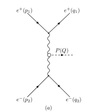
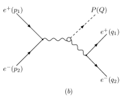
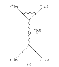
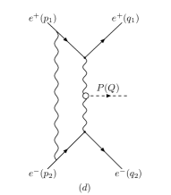
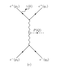
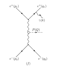
Figure 1: Representative sample of diagrams contributing to the amplitude $e^{+}e^{-}\to e^{+}e^{-}P(\gamma)$.

The vacuum polarisation corrections are included in a fully factorised and resummed form

$$\kern-30.0ptM_{LO+virt}(e^{+}e^{-}\to e^{+}e^{-}P)\to M_{LO+virt}\cdot\frac{1}{1-\Delta\alpha(t_{1})}\cdot\frac{1}{1-\Delta\alpha(t_{2})}\,,$$

$$\kern-30.0ptM_{e+f}(e^{+}e^{-}\to e^{+}e^{-}P\gamma)\to M_{e+f}(e^{+}e^{-}\to e^{+}e^{-}P\gamma)\cdot\frac{1}{1-\Delta\alpha(t_{1}^{\prime})}\cdot\frac{1}{1-\Delta\alpha(t_{2})}\,,$$

(4)

with $t_{2}=(p_{2}-q_{2})^{2}$, $t_{1}^{\prime}=(p_{1}-q_{1}-k)^{2}$. Analogously one adds the radiative corrections to the diagrams with a photon emitted from the electron lines. The $\Delta\alpha(t)$ is taken from [25] (see also [26, 27]).

3.2 Real radiative corrections

The matrix element describing the reaction

$$e^{+}(p_{1})e^{-}(p_{2})\to e^{+}(q_{1})e^{-}(q_{2})P(Q)\gamma(k)$$ (5)

was calculated using Feynman diagrams shown in Fig. 1 (e) and (f) and similar diagrams, where photon is emitted from the electron line. As stated already, the five point functions (Fig. 1 (d)) were found negligible [23]. They cancel the infrared singularities from the interference between the diagrams with the photon emitted from the positron lines and with the photon emitted from the electron lines. Thus that interference has to be neglected for consistency.

It is convenient to parameterise the phase space of the reaction Eq.(5) in the following way [28]

$$\kern-30.0pt\int dLips_{4}(p_{1}+p_{2};q_{1},q_{2},Q,k)=$$

$$\kern-15.0pt\frac{1}{(2\pi)^{8}}\frac{1}{4\sqrt{\lambda(s,m_{e}^{2},m_{e}^{2})}}\int\displaylimits_{(m_{P}+m_{e}+m_{\gamma})^{2}}^{(\sqrt{s}-m_{e})^{2}}dM_{3}^{2}\int\displaylimits_{t_{3}^{-}}^{t_{3}^{+}}dt_{3}\int\displaylimits_{0}^{2\pi}d\phi_{2}$$

$$\kern-15.0pt\frac{1}{4\sqrt{\lambda(M_{3}^{2},t_{3},m_{e}^{2})}}\int\displaylimits_{(m_{e}+m_{\gamma})^{2}}^{(M_{3}-m_{P})^{2}}dM_{2}^{2}\int\displaylimits_{t_{2}^{-}}^{t_{2}^{+}}dt_{2}\int\displaylimits_{0}^{2\pi}d\phi_{P}\frac{1}{4\sqrt{\lambda(M_{2}^{2},t_{2},m_{\gamma}^{2})}}\int\displaylimits_{t_{1}^{-}}^{t_{1}^{+}}dt_{1}\int\displaylimits_{0}^{2\pi}d\phi_{1}\,,$$

(6)

with

$$\lambda(a,b,c)=a^{2}+b^{2}+c^{2}-2ab-2ac-2bc\,,\ \ \ t_{1}=(p_{1}-k)^{2}\,,$$

$$M_{3}^{2}=(Q+k+q_{1})^{2}=(p_{1}+p_{2}-q_{2})^{2}\,,\ \ \ \ \ \ \ t_{3}=(p_{2}-q_{2})^{2}\,,$$

$$M_{2}^{2}=(k+q_{1})^{2}=(p_{1}+p_{2}-q_{2}-Q)^{2}\,,\ \ \ \ \ \ \ t_{2}=(p_{2}-q_{2}+Q)^{2}\,,$$

(7)

$m_{P},m_{e}$ and $m_{\gamma}$ being pseudoscalar, electron and a fictitious photon mass, respectively, and

$$t_{3}^{\pm}=m_{e}^{2}+M_{3}^{2}-\frac{1}{2s}\left\{s(s+M_{3}^{2}-m_{e}^{2})\mp\sqrt{\lambda(s,m_{e}^{2},m_{e}^{2})\lambda(s,M_{3}^{2},m_{e}^{2})}\right\}\,,$$

$$t_{2}^{\pm}=m_{e}^{2}+M_{2}^{2}-\frac{1}{2M_{3}^{2}}\Bigg{\{}(M_{3}^{2}+m_{e}^{2}-t_{3})(M_{3}^{2}+M_{2}^{2}-m_{P}^{2})$$

$$\kern 160.0pt\mp\sqrt{\lambda(M_{3}^{2},m_{e}^{2},t_{3})\lambda(M_{3}^{2},M_{2}^{2},m_{P}^{2})}\Bigg{\}}\,,$$

$$t_{1}^{\pm}=m_{e}^{2}+m_{\gamma}^{2}-\frac{1}{2M_{2}^{2}}\Bigg{\{}(M_{2}^{2}+m_{e}^{2}-t_{2})(M_{2}^{2}+m_{\gamma}^{2}-m_{e}^{2})$$

$$\kern 160.0pt\mp\sqrt{\lambda(M_{2}^{2},m_{e}^{2},t_{2})\lambda(M_{2}^{2},m_{\gamma}^{2},m_{e}^{2})}\Bigg{\}}\,.$$

(8)

In this way all the peaks appearing in the matrix element can be easily absorbed for the contributions from Fig. 1 (e) and (f). To do that we use the following changes of variables

$$t_{i}=-e^{-z_{i}},i=2,3;\ \ \ M_{2}^{2}=m_{e}^{2}+e^{y};\ \ \ t_{1}=m_{e}^{2}-e^{-z_{1}}\,.$$ (9)

In the above formulae, $e^{a}$ should be read as $1$ GeV${}^{2}\cdot e^{a}$. For simplicity, the unit $1$ GeV² was dropped in all formulae.

The first two changes of variables absorb peaks coming from the virtual photons propagators, the third (fourth) one the peak coming from the positron propagator in the diagram with photon emitted from final (initial) positron line. The last two changes of variables have to be present simultaneously as the leading contribution comes from the interference of the diagram (e) and the diagram (f).

The user introduced cuts on $t_{3}$ are used to alter the generation limits. Other user cuts are just rejecting events generated outside the allowed phase space. The cuts on $t_{3}^{min}<t_{3}<t_{3}^{max}$ change the maximal allowed value of $M_{3}$ ( $M_{3}^{max}$) if both $t_{3}^{min}$ and $t_{3}^{max}$ are bigger (lower) than $t_{3}^{c}=2m_{e}^{2}-\sqrt{s}m_{e}$. It reads

$$M_{3,max}^{2}=\frac{2m_{e}^{4}+t_{3}^{min}s+\sqrt{\Delta(t_{3}^{min})}}{2m_{e}^{2}}\ ,\ \ {\rm for}\ \ t_{3}^{min}>t_{3}^{c},t_{3}^{max}>t_{3}^{c}$$

$$M_{3,max}^{2}=\frac{2m_{e}^{4}+t_{3}^{max}s+\sqrt{\Delta(t_{3}^{max})}}{2m_{e}^{2}}\ ,\ \ {\rm for}\ \ t_{3}^{min}<t_{3}^{c},t_{3}^{max}<t_{3}^{c}$$ (10)

with $\Delta(t)=ts(t-4m_{e}^{2})(s-4m_{e}^{2})$.

As the matrix element contains also the contributions coming from the photons emitted from the electron line we use two-channel Monte Carlo, where in the second channel the parameterisation of the phase space is identical to the one described above with the change $p_{2}\leftrightarrow p_{1}$ and $q_{2}\leftrightarrow q_{1}$. Within that two-channel scheme the phase space parameterisation is written as

$$\int dLips_{4}(p_{1}+p_{2};q_{1},q_{2},Q,k)=\int\displaylimits_{0}^{1}dr_{0}\left[\theta\left(\frac{1}{2}-r_{0}\right)C_{1}+\theta\left(r_{0}-\frac{1}{2}\right)C_{2}\right]$$

(11)

with $\theta$ being a Heaviside step function and $C_{i},\ \ i=1,2$ the parameterisations of the phase space in channels $1$ and $2$. The parameterisation in the channel $1$ reads

$$\kern-15.0ptC_{1}=\frac{1}{(2\pi)^{5}}\frac{\Delta M_{3}^{2}}{2\sqrt{\lambda(s,m_{e}^{2},m_{e}^{2})}}\int\displaylimits_{0}^{1}dr_{1}\int\displaylimits_{0}^{1}dr_{2}\frac{\Delta z_{3}}{4\sqrt{\lambda(M_{3}^{2},t_{3},m_{e}^{2})}}$$

$$\kern-15.0pt\cdot\int\displaylimits_{0}^{1}dr_{3}\int\displaylimits_{0}^{1}dr_{4}\frac{\Delta y\Delta z_{2}}{4\sqrt{\lambda(M_{2}^{2},t_{2},m_{\gamma}^{2})}}\int\displaylimits_{0}^{1}dr_{5}\frac{\Delta z_{1}}{f_{1}+f_{2}}\int\displaylimits_{0}^{1}dr_{6}\int\displaylimits_{0}^{1}dr_{7}\int\displaylimits_{0}^{1}dr_{8}\,,$$

(12)

where

$$M_{3}^{2}=M_{3,min}^{2}+\Delta M_{3}^{2}\cdot r_{1},\ \ \Delta M_{3}^{2}=M_{3,max}^{2}-M_{3,min}^{2}\,,$$

$$z_{3}=z_{3}^{min}+\Delta z_{3}\cdot r_{2},\ \ z_{2}=z_{2}^{min}+\Delta z_{2}\cdot r_{4},\ \ z_{1}=z_{1}^{min}+\Delta z_{1}\cdot r_{5}\,,$$

$$z_{i}^{min}=-\log(-t_{i}^{min}),\ \ \Delta z_{i}=-\log\left(\frac{t_{i}^{max}}{t_{i}^{min}}\right),\ \ i=2,3$$

$$z_{1}^{min}=-\log(-\tilde{t}_{1}^{min}),\ \ \Delta z_{1}=-\log\left(\frac{\tilde{t}_{1}^{max}}{\tilde{t}_{1}^{min}}\right)\,,$$

$$\tilde{t}_{1}^{max(min)}=m_{\gamma}^{2}$$

$$-\frac{(M_{2}^{2}+m_{e}^{2}-t_{2})(M_{2}^{2}+m_{\gamma}^{2}-m_{e}^{2})+(-)\lambda^{1/2}(M_{2}^{2},m_{e}^{2},t_{2})\lambda^{1/2}(M_{2}^{2},m_{e}^{2},m_{\gamma}^{2})}{2M_{2}^{2}}\,,$$

$$y=y_{min}+\Delta y\cdot r_{3},\ \ y_{min}=\log(m_{\gamma}(2m_{e}+m_{\gamma}))\,,$$

$$\Delta y=\log\left(\frac{(M_{3}-m_{P})^{2}-m_{e}^{2}}{m_{\gamma}(2m_{e}+m_{\gamma})}\right),t_{1}=\tilde{t}_{1}+m_{e}^{2}\,,$$

$$\kern-15.0ptf_{1}=\frac{-1}{t_{3}(M_{2}^{2}-m_{e}^{2})t_{2}(t_{1}-m_{e}^{2})},\ \ \phi_{2}=2\pi\cdot r_{6},\ \ \phi_{P}=2\pi\cdot r_{7},\ \ \phi_{1}=2\pi\cdot r_{8}\,.$$

(13)

The function $f_{2}$ is obtained with $f_{1}$ with the change $p_{2}\leftrightarrow p_{1}$ and $q_{2}\leftrightarrow q_{1}$. The parameterisation of the phase space in the second channel ($C_{2}$) is obtained from $C_{1}$ with the same substitutions.

From the generated variables described above one can calculate the four-momenta of all final particles. Again, we give here only formulae for the channel 1 as the channel 2 is obtained in the same way with the substitutions $p_{2}\leftrightarrow p_{1}$ and $q_{2}\leftrightarrow q_{1}$. Moreover, as it is possible to write some of the expressions given below in two or more analytically equivalent forms, we give here only the ones used in the code. They were chosen to obtain formulae which are numerically stable.

The azimuthal angle of the final electron ($\phi_{2}$) is generated in the initial $e^{+}e^{-}$ center of mass frame with positron momentum along the z-axis: $p_{1}=(\sqrt{s}/2,0,0,p)$, $p=\sqrt{s/4-m_{e}^{2}}$. This frame is called the LAB frame from now on. The energy ($E_{2}$), the length of the momentum ($lq_{2}$) and the cosine of the polar angle ($\theta_{2}$) of the final electron can be calculated, in the same frame, from the generated invariants

$$\kern-30.0ptE_{2}=\frac{s-M_{3}^{2}+m_{e}^{2}}{2\sqrt{s}},\ \ lq_{2}=\frac{\lambda^{1/2}(M_{3}^{2},s,m_{e}^{2})}{2\sqrt{s}},\ \ \cos(\theta_{2})=\frac{M_{3}^{2}-s-2t_{3}+3m_{e}^{2}}{4\cdot p\cdot lq_{2}}\,.$$

(14)

The azimuthal angle of the pseudoscalar ($\phi_{P}$) is generated in the rest frame of the four-vector $p_{1}+p_{2}-q_{2}$, where the z-axis is pointing the initial positron momentum $p_{1}=(\tilde{E}_{1},0,0,\tilde{p}_{1})$. Here $\tilde{E}_{1}=\frac{M_{3}^{2}+m_{e}^{2}-t_{3}}{2M_{3}}$. In this frame $p_{2}-q_{2}=(\tilde{E}_{2},0,0,-\tilde{p}_{1})$, with $\tilde{E}_{2}=\frac{M_{3}^{2}-m_{e}^{2}+t_{3}}{2M_{3}}$. In the code, for numerical stability reasons, the expression $\tilde{p}_{1}=\sqrt{\tilde{E}_{2}^{2}-t_{3}}$ is used to calculate $\tilde{p}_{1}$. In this frame, the pseudoscalar energy ($E_{P}$), the length of the pseudoscalar momentum ($lq_{P}$) and the cosine of the pseudoscalar polar angle ($\theta_{P}$) are given by

$$\kern-30.0ptE_{P}=\frac{M_{3}^{2}-M_{2}^{2}+m_{P}^{2}}{2M_{3}},\ \ lq_{P}=\sqrt{E_{P}^{2}-m_{P}^{2}},$$

$$\kern-30.0pt\cos(\theta_{P})=\frac{t_{3}-t_{2}+m_{P}^{2}-\frac{(M_{3}^{2}-m_{e}^{2}+t_{3})(M_{3}^{2}-M_{2}^{2}+m_{P}^{2})}{2M_{3}^{2}}}{2\cdot\tilde{p}_{1}\cdot lq_{P}}\,.$$ (15)

After being calculated, the pseudoscalar four vector is transformed into the LAB frame.

The azimuthal angle of the final positron ($\phi_{1}$) is generated in the rest frame of the four-vector $p_{1}+p_{2}-q_{2}-Q$, where the z-axis is pointing the initial positron momentum $p_{1}=(E_{1}^{*},0,0,p_{1}^{*})$. Here $E_{1}^{*}=\frac{M_{2}^{2}+m_{e}^{2}-t_{2}}{2M_{2}}$. In this frame $p_{2}-q_{2}-Q=(E_{2}^{*},0,0,-p_{1}^{*})$ with $E_{2}^{*}=\frac{e^{y}+t_{3}}{2M_{3}}$. In the code the expression $p_{1}^{*}=\sqrt{E_{2}^{*,2}-t_{2}}$ is used to calculate $p_{1}^{*}$. The $p_{1}+p_{2}-q_{2}-Q$ rest frame is also the $q_{1}+k$ rest frame, thus the final positron and the final photon momenta differ only by a sign. In this frame, the final positron energy ($E_{1}$), the length of its momentum ($lq_{1}$), the cosine of its polar angle ($\theta_{1}$) and the photon energy ($E_{\gamma}$) are given by

$$\kern-30.0ptE_{1}=\frac{M_{2}^{2}-m_{\gamma}^{2}+m_{e}^{2}}{2M_{2}},\ \ lq_{1}=\frac{\sqrt{(e^{y}+m_{\gamma}^{2}-2m_{\gamma}M_{2})(e^{y}+m_{\gamma}^{2}+2m_{\gamma}M_{2})}}{2M_{2}},$$

$$\kern-30.0ptE_{\gamma}=\frac{e^{y}+m_{\gamma}^{2}}{2M_{2}},\ \ \cos(\theta_{1})=\frac{m_{e}^{2}+m_{\gamma}^{2}-\frac{(e^{y}+m_{\gamma}^{2})(M_{2}^{2}+m_{e}^{2}-t_{2})}{2M_{2}^{2}}}{2\cdot p_{1}^{*}\cdot lq_{1}}\,.$$ (16)

From the rest frame of the $p_{1}+p_{2}-q_{2}-Q$ four-momentum to the LAB frame the four vectors are transformed in two steps. First to the $p_{1}+p_{2}-q_{2}$ rest frame and than to the LAB frame. In this way the same subroutine can be used for both transformations. It consists of a boost and three elementary rotations. It was checked numerically that, after transforming all four vectors to the LAB frame, $q_{1}+q_{2}+Q+k=p_{1}+p_{2}$ within 28-digits accuracy.

3.3 Tests of the code

The code is using in its bulk part the quadruple numerical precision, with exceptions described in Section 5. All the tests described below were performed with a precision of one half of a per mile or better. We cover here only the tests of the newly developed part. The tests of the previously developed parts of the code are covered in [29, 17, 15, 20].

The matrix element of the LO contribution to the cross section of the reaction $e^{+}e^{-}\to e^{+}e^{-}P$ was tested in [17], thus one does not have to test the part of the virtual radiative corrections $\sim F_{1}$ as they are proportional to the same matrix element. The part of the virtual radiative corrections proportional to $F_{2}$ was calculated, using trace method to sum over polarisations, independently by two of the authors. As this contribution is negligible, no further tests were performed.

For the matrix element describing the reaction $e^{+}e^{-}\to e^{+}e^{-}P\gamma$ two independent codes were constructed. One using helicity amplitude method, where sum over helicities was done numerically, and one using trace method to sum over polarisations. For the calculations using trace method the symbolic manipulation system FORM [30] was used and a FORTRAN code was produces based on its output. Even if the code uses quadruple precision, the code constructed using the trace method is not numerically stable around kinematical points with few invariants appearing in the denominators of the expression being close to zero simultaneously. As there are almost no numerical cancellations in the formulae, which use the helicity amplitude method, these formulae are free from such problems. An agreement up to 28 digits was found between the results obtained with the two described methods for all the phase space points with the exception of the situations described above. The formula, which uses the helicity amplitude method is used in the distributed version of the code.

The phase space parameterisation, together with the change of variables described in Section 3.2, was tested comparing the phase space volume calculated within that parameterisation and the volume calculated with an independent code, which uses a flat cascade-like parameterisation [28]. A very good agreement was found for all tested energies, in the range $1\ GeV<\sqrt{s}<11\ GeV$, and for physical masses of the pseudoscalar particles ($\pi^{0},\eta,\eta^{\prime}$).

The differential cross sections, when one sums the contributions with and without a real photon emission should not depend on the fictitious photon mass ($m_{\gamma}$) introduced as a regulator. We use a parameter $\lambda$ ($m_{\gamma}=\lambda m_{e}$) to set its size in the code. The recommended value for $\lambda$ is 0.01. For $\lambda\sim 0.1$ some of the differential cross sections start to depend on this parameter with deviations bigger than the one set as a goal for technical accuracy in this code (0.05%). For $\lambda=0.001$ and $\lambda=0.0001$ the differential cross sections were identical to the one obtained with $\lambda=0.01$ within the errors of about 0.05%. Due to this small cut-off, the infrared divergent part in the virtual corrections, which is negative, is bigger than 1 resulting in the negative cross section. As a result, one cannot generate unweighted event sample and only weighted events can be used.

4 The size of the radiative corrections and comparisons with GGRESRC Monte Carlo generator

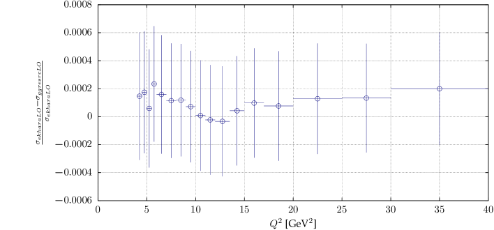
Figure 2: Comparison of the EKHARA and GGRESRC generators at LO;                               $Q^{2}=-(p_{1}-q_{1})^{2}$, $\sqrt{s}=10.58{\rm GeV}$.

There exists a Monte Carlo event generator [13], GGRESRC, were the radiative corrections to the reaction $e^{+}e^{-}\to e^{+}e^{-}P$ were included using a structure function method. This generator was used in the BaBar analysis to measure the $\gamma-\gamma^{*}-P$ transition form factors [9, 10]. The accuracy of the structure function method depends a lot on the event selection (see for example [14]). It is thus important to check it against exact calculations, whenever possible. For simulation of the reaction $e^{+}e^{-}\to e^{+}e^{-}P$, at LO level the EKHARA and GGRESRC Monte Carlo generators are very similar. When the same form factor is used in both codes we have observed an agreement at a level of 0.04%. This was already observed in [13] for $e^{+}e^{-}\to e^{+}e^{-}\pi^{0}$. We have checked that also for $\eta$ and $\eta^{\prime}$ integrated cross sections, angular and energy distributions of all final particles are identical for both generators in a single tag mode. To obtain this agreement a VMD transition form factor used in GGRESRC was implemented in the EKHARA Monte Carlo generator. In all the comparisons between the generators shown in this paper that form factor is used. An example of these comparisons is shown in Fig. 2. We have restricted the invariant $-0.18\ {\rm GeV^{2}}<(p_{2}-q_{2})^{2}<0\ {\rm GeV^{2}}$ and calculated the cross section in bins of $Q^{2}=-(p_{1}-q_{1})^{2}$ as shown in Fig. 2. The bins coincide with the bins used by BaBar collaboration [9].

At NLO it is not a straightforward task to compare the two event generators as in the formulae used in GGRESRC generator the ’final’ photon is integrated out. The final photon would come from the the diagram Fig. 1 (f). Yet the interference between the amplitudes coming from Fig. 1 (e) and Fig. 1 (f) gives substantial contributions to the matrix element squared and the identification ’final’ or ’initial’ photon is not possible. One could of course define the final or initial photon on the bases of being closer to the initial or final lepton, but then one would need to integrate the photons which are closer to the final lepton, to be close to the formulae used in GGRESRC generator. There is one more difference between the generators: in GGRESRC the corrections to the line of the untagged lepton are not included. We thus start with the check how big they are in the EKHARA generator to disentangle these two different effects. We do it for the event selection close to the one used by BaBar. We use here kinematical variables (angles, energies) in the center of mass frame of the initial leptons. We require that the final positron and pion polar angles are in the range $20^{\circ}<\theta_{\pi,e}<160^{\circ}$. We also put cuts on polar angle of $\pi^{0}e^{+}$ system $\cos(\theta_{e\pi})>0.99$ and on a variable $r=(\sqrt{s}-E_{e\pi}-p_{e\pi})/\sqrt{s}<0.075$.

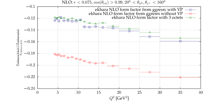
Figure 3: The size of the radiative corrections predicted with EKHARA Monte Carlo generator.

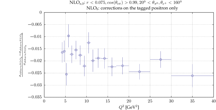
Figure 4: The complete corrections compared to the corrections only to the tagged lepton line.

The results are shown in Fig. 3. The complete radiative corrections for that event selection are negative and amount from 12 % to 16% depending on the range of the $Q^{2}$ invariant. The corrections coming from photon vacuum polarisation amount, for this event selection, to 6-7.5% depending on the tagged invariant and are positive. The size of the corrections depends only slightly on the form factor, as shown in Fig. 3. The cross sections predicted with these two different form factors differ up to 35%. Yet, the radiative corrections as a fraction of LO cross section differ at most by 1%. The form factors used in this comparison were: the VDM form factor from GGRESRC generator and the form factor based on 3 octet model from [16].

If we switch off the corrections to the untagged electron line we find out that indeed, as stated in [13], the dominant contribution comes from the tagged line. The difference, amounting to 1.5-2.5 %, is shown in Fig. 4.

One has to mention here that the $Q^{2}=-(p_{1}-q_{2})^{2}$ is not the invariant for which the form factor is calculated. The correct invariant reads $(p_{1}-q_{1}-k)^{2}$. The imposed cuts assure that the second invariant is close to zero. The size of the radiative corrections, if one uses the correct invariant, is also different. Yet, the difference is small, as shown in Fig. 5.

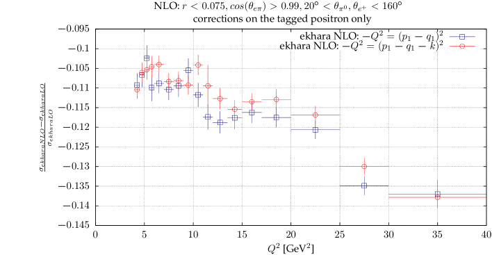
Figure 5: The size of radiative corrections compared for binning in variable $Q^{2}=-(p_{1}-q_{1}-k)^{2}$ and $Q^{2}=-(p_{1}-q_{1})^{2}$.

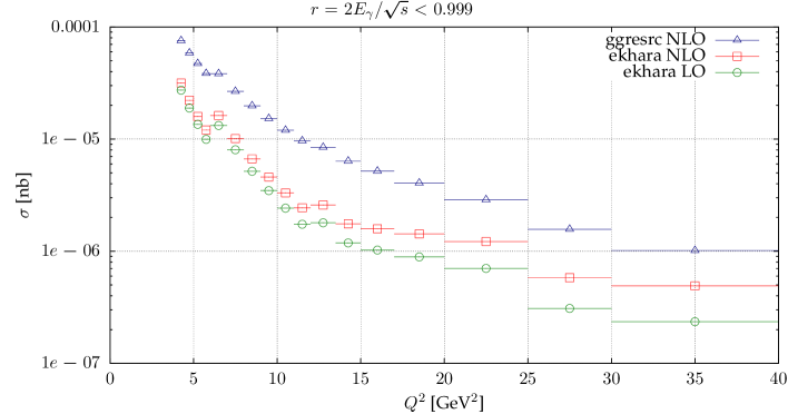
Figure 6: Comparison between EKHARA and GGRESRC Monte Carlo generators.

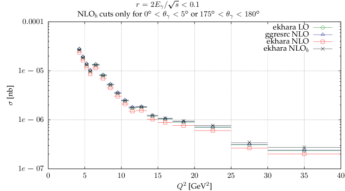
Figure 7: Comparison between EKHARA and GGRESRC Monte Carlo generators.

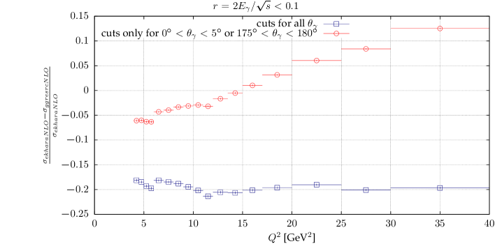
Figure 8: Comparison between EKHARA and GGRESRC Monte Carlo generators.

As the TREBSBST [12] generator is not publicly available in its version with radiative corrections, we compare here only our results with GGRESRC generator. To see the differences in the NLO predictions between the EKHARA and GGRESRC event generators, we show in Fig. 6 the results with no direct angular cuts and the untagged invariant in the range $-0.18\ {\rm GeV^{2}}<(p_{2}-q_{2})^{2}<0$, as a function of the tagged invariant. We do not impose any cut on the emitted photon energy in EKHARA and use Rmax=0.999 in GGRESRC. This should correspond to the situation were one does not include any direct cut on the photon variables. Big differences are observed. We were not able to trace back the source of the difference.

Smaller differences are observed (Fig. 7), when one imposes a cut-off on the photon energy. Yet, as in GGRESRC the photons are partly integrated, the compared cross sections are not defined identically and one cannot expect a complete agreement. To come closer to the GGRESRC we have applied cuts on the photon energy only if the photon polar angles are within 5 degrees from the initial leptons direction. The results are also shown in Fig. 7. As expected the results come closer, yet they are not in agreement. The relative difference is shown in Fig. 8.

5 The software structure and the users guide

5.1 An overview of the code structure

The overview of the code structure is given here and for completeness we repeat in part the description given in [17]. A more detailed users guide is a part of the distributed package.

Let us start with an overview of the directory structure of the distribution. EKHARA is distributed as a source code. The code of the Monte Carlo generator is located in the directory ekhara-routines. The main source file of EKHARA is ekhara.for. There are other source files in the directory ekhara-routines, which are automatically included:

• the $e^{+}e^{-}\to e^{+}e^{-}P$ modes are implemented in routines_1pi.inc.for and its supplementary histograming routines are given in routines-histograms_1pi.inc.for;

• the $e^{+}e^{-}\to e^{+}e^{-}\pi^{+}\pi^{-}$ mode is coded in routines_2pi.inc.for, its supplementary histograming routines are in routines-histograms_2pi.inc.for and helicity-amplitude routines are given in routines-helicity-aux.inc.for;

• the $e^{+}e^{-}\to e^{+}e^{-}\chi_{c_{i}}$ and $e^{+}e^{-}\to e^{+}e^{-}\chi_{c_{i}}(\to J/\psi(\to\mu^{+}\mu^{-})\gamma)$ modes are implemented in routines_chi.inc.for and its supplementary histograming routines are given in routines-histograms_chi.inc.for;

• the NLO corrections to $e^{+}e^{-}\to e^{+}e^{-}P$ modes are implemented in routines_1pi_1ph.inc.for. It uses partly routines from routines_1pi.inc.for. Its supplementary histograming routines are given in routines-histograms_1pi.inc.for;

• the routines for the matrix and vector manipulations are located in routines-math.inc.for;

• in routines-user.inc.for several routines, which can be changed by a user in order to customise the operation of EKHARA, are collected; they handle the data-card reading, the reporting of events, the form factor evaluation, the filling of the histograms, the application of additional phase space cuts, etc.;

• all common blocks are included from the file common.ekhara.inc.for. This file contains the detailed comments on the explicit purpose of the most important common variables.

• the routines from the package alphaQEDc17 [25] to calculate the vacuum polarisation corrections are contained in files: common.h,constants.f,constants_qcd.f,dalhadshigh17.f,
  dalhadslow17.f, dalhadt17.f,dggvapx.f,hadr5n17.f,leptons.f,
  vacpol_alphaQEDc17.inc.for

The operation of the EKHARA generator requires the following steps:

1. the initialisation,

2. the event generation,

3. the finalisation.

The main directory of the distributed version contains a readme.txt file with a short description how to compile, run and test the program in the regimes described above. It is suggested to use the Makefile, which is placed in the main directory. An example of the full set of input files and the plotting environment is supplied in the Env sub-directory. If one uses the distributed Makefile, the content of the Env sub-directory will be put into the EXE sub-directory together with an executable ekhara.exe.

5.2 the I/O scheme and files

All the input files of EKHARA are supposed to be located in the same directory as the main executable, ekhara.exe. There are the following types of the input files: random seeds, the parameter input, data-cards and histogram settings. An example of the full set of input files can be found in the Env directory.

All the output files of EKHARA are written into ./output sub-directory. There are the following types of the output files: logs of execution, histograms and events.

The input files

The main input file is called input.dat. It contains all global settings, which are explained in this file as well.

The channel-dependent parameters are collected in “data-cards” card_1pi.dat, card_2pi.dat and card_chi.dat. These data-cards allow to set the total energy, types of included amplitudes and kinematic cuts. A detailed description can be found in comments within these files. In card_1pi.dat one can also use the piggFFsw switch in order to select the form of the two photon pseudoscalar transition form factor. The recommended values are 9 or 10 as these are the form factors which were fitted to the widest data set [16], both in the space-like and time-like regions.

The channel-dependent histograming settings are given in the files histo-settings_1pi.dat, histo-settings_2pi.dat, histo-settings_chi.dat and histo-settings_1pi_1ph.dat.

The output and the logging

The main execution log file is output/runflow.log. It contains main information about the operation mode and status of EKHARA, this information is also partly written into the standard output (i.e., the console). At the end of a successful execution, the total cross section is reported to output/runflow.log and also to the standard output.

A non-standard behaviour of the MC generator is reported into output/warnings.log, while the critical problems in the event generator operation are reported into the file output/errors.log.

In the case of a correct operation, output/errors.log and output/warnings.log should remain empty. We strongly recommend to keep track on this issue and report to the authors any warnings or errors. In the NLO mode one can ignore warnings about negative weights in the part without a photon. Yet in this case only weighted events can be used.

The output: histograms and plotting scripts

When histograming is allowed through settings in the input.dat, the plain text files with the histogram data are saved at the end of the generator execution.

• In the $e^{+}e^{-}\to e^{+}e^{-}\pi^{+}\pi^{-}$ mode the file histograms_2pi.out contains the data for $d\sigma/dQ^{2}$ histogram. One may use the plotting script doplots.sh from directory histo-plotting_2pi in order to plot this histogram (an installed Gnuplot is required).

• In the $e^{+}e^{-}\to e^{+}e^{-}P$ modes there is a wide set of histograms stored in the files histo<Number>.<variable>.dat, where <Number> stands for the histogram number and <variable> is the histograming variable acronym.

  One can use the plotting script do-everything.sh in the directory histo-plotting_1pi in order to plot all the histograms and collect them into a single postscript file. An installed LaTeX system is required for the latter.

  One can use the plotting script doplots.sh in the directory t1-t2-bars_1pi in order to plot the 3D-bar graph, which shows the event distribution in two variables: $t_{1}$ and $t_{2}$.

  In the NLO mode the files histo_th_electron.dat, histo_th_positron.dat and histo_th_pseudoscalar.dat contain the data for $\Delta\sigma$ in the polar angles $\Delta\theta_{e^{-}}$, $\Delta\theta_{e^{+}}$ and $\Delta\theta_{\pi^{0},\eta,\eta^{\prime}}$ histograms respectively. $\Delta\sigma$ is the integrated cross section in a given bin.

  One can use the plotting script do-everything.sh in the directory histo-plotting_1pi_1ph to plot all the histograms and collect them into a single postscript file.

• In the $e^{+}e^{-}\to e^{+}e^{-}\chi_{c_{i}}$ and $e^{+}e^{-}\to e^{+}e^{-}\chi_{c_{i}}(\to J/\psi(\to\mu^{+}\mu^{-})\gamma)$ modes the file histograms_chi.out contains the data for $d\sigma/dQ^{2}$ histogram.

  One can use the plotting script doplots.sh in the directory histo-plotting_chi in order to plot histogram and to obtain a single postscript file.

As the histograms are stored as plain text files the user can use also her/his favourite plotting programs to visualise the histograms.

The output: events

The generated four-momenta of the particles are stored in the following variables accessible through common blocks:

p1	initial positron,
p2	initial electron,
q1	final positron,
q2	final electron,
qpion	final pseudoscalar ($e^{+}e^{-}\to e^{+}e^{-}P(\gamma)$ modes),
k_hp	final photon ($e^{+}e^{-}\to e^{+}e^{-}P\gamma$ modes),
qu	final $\chi_{c_{i}}$ ($e^{+}e^{-}\to e^{+}e^{-}\chi_{c_{i}}$ modes),
q3	final $\mu^{-}$ in $e^{+}e^{-}\to e^{+}e^{-}\chi_{c_{i}}(\to J/\psi(\to\mu^{+}\mu^{-})\gamma)$ modes),
q4	final $\mu^{+}$ in $e^{+}e^{-}\to e^{+}e^{-}\chi_{c_{i}}(\to J/\psi(\to\mu^{+}\mu^{-})\gamma)$ modes),
k1	final photon in $e^{+}e^{-}\to e^{+}e^{-}\chi_{c_{i}}(\to J/\psi(\to\mu^{+}\mu^{-})\gamma)$ modes),
pi1, pi2	final pseudoscalars ($e^{+}e^{-}\to e^{+}e^{-}\pi^{+}\pi^{-}$ mode).
contribute	weights NLO.

The weights in the NLO mode allow to calculate a cross section, given in nanobarns, for any event selection using a formula $\Delta\sigma_{k}=\frac{\sum_{i}w_{i}}{N_{k}}$, with $k=0,1$, where $k=0$ stands for events without a photon and $k=1$ stands for events with one photon. In the output the k_hp is a zero four vector for events without a photon. $w_{i}$ is the weight, $N_{0}$ is the number of events with no photons and $N_{1}$ is the number of events with one photon. The sum span over all events for a given event selection.

In the standalone regime we suggest to use the routine reportevent_1pi defined in the file routines-user.inc.for, which is called automatically for every accepted unweighted event ($e^{+}e^{-}\to e^{+}e^{-}P$ modes only). In the NLO mode the routine reportevent_1pi_1ph, defined in this same file, reports every event used to calculate the cross section from the weighted events. In the chi_c modes the routine reportevent_chi, which can be found in the file routines-user.inc.for, reports momenta for every accepted unweighted event. In the distributed version this routine writes the events to the file output/events.out when WriteEvents flag is on.

5.3 Selected procedures

The top-level interface to the Monte Carlo generator is provided by the routine

EKHARA(i)

i = -1: initialise, i = 0: generate event(s), i = 1: finalise.

Only this routine should be called from an external program, when one uses EKHARA in the event-by-event regime. An example is provided in ekhara-call-example.for.

In order to describe briefly the “internal” structure of EKHARA, we list several important routines.

EKHARA_INIT_read	the reading the input files and datacards,
EKHARA_INIT_set	the initialisation of the MC loop and mappings,
EKHARA_RUN	the MC loop execution,
EKHARA_FIN	the MC finalisation and the saving the results.

5.4 Compilation instructions

Being distributed as a source code the program does not require installation, but a compilation and a linking are needed. EKHARA does not need any specific external libraries, but requires

• a FORTRAN 77 compiler which supports the quadruple precision,

• a C compiler.

The current version of the program was tested on the following platforms : Linux (Ubuntu 14.04, Ubuntu 16.04).

The program distribution contains the Makefile, with targets: default64 - to built a standalone version of the MC generator, all64 - to compile everything including default, ranlux-testing program and seed-production and test64 - to compile everything and execute the test run scripts.

A simple way to compile the program is to issue make default64, being in the directory where the Makefile is located. This will produce ekhara.exe (the main program executable) and copy it into the sub-directory EXE, together with the content of the Env sub-directory. The latter contains the set of sample input files and histogram plotting scripts. We provide a full set of necessary input files in the distribution package. It is advised to execute ekhara.exe in the directory EXE, where it is placed by default. Every time one executes make default64, the input files in the directory EXE are replaced with the sample ones from the directory Env.

EKHARA needs a random seed for operation. Different random seeds can be obtained by using the Makefile target seed_prod-ifort. It produces an executable program seed_prod.exe, which generates a set of random seeds.

5.5 A test run description

It is recommended to test the random number generator on a given machine, before using EKHARA. It is also important to check whether EKHARA can function properly on a given operational system and that there are no critical bugs due to the compiler. We provide a test run package for these purposes.

It is suggested to use the Makefile target test64. This will automatically prepare and execute the following two test steps.

The first step of the test run is the random number generator control. The source file testlxf.for contains the ranlux test routines. The random numbers are the only part of the code used in double precision.

The second step is the verification if the user-compiled EKHARA can reproduce the set of results, created by a well-tested copy of EKHARA in various modes. The test run environment contains directory test with pre-calculated data for the comparison, the random seed and input files for each mode. The script test.sh executes the user-compiled ekhara.exe in all the control modes and compares the output with previously stored results.

Please read carefully the output of the test run execution in your console and be sure there are no warnings and/or error messages.

5.6 A customisation of the source code by a user

We leave for a user an option to customise the generator to her/his needs by editing the source code file ekhara-routines/routines-user.inc.for. Notice that we always use explicit declaration of identifiers and the implicit none statement is written down in each routine.

In the file ekhara-routines/routines-user.inc.for one can change

• the data-card reading (routines read_card_1pi, read_card_2pi and read_card_chi),

• the form-factor formula (routine piggFF),

• the events reporting (routines reportevent_1pi, reportevent_1pi_1ph and reportevent_chi),

• the histograming (routines histo_event_1pi, histo_event_2pi, histo_event_1pi_0ph and histo_event_1pi_1ph),

• additional kinematic cuts (routines ExtraCuts_1pi and ExtraCuts_2pi).

6 Conclusions

In this paper we have presented the upgrades of the EKHARA Monte Carlo generator. The main result being the radiative corrections to the reactions $e^{+}e^{-}\to e^{+}e^{-}P$, with a new algorithm of the phase space generation for the reaction $e^{+}e^{-}\to e^{+}e^{-}P\gamma$. Comparisons with GGRESRC generator are also shown. Big differences are observed between the radiative corrections calculated by the EKHARA generator, which uses NLO exact formulae and the GGRESRC generator based on the structure function approach.

7 Acknowledgements

We would like to thank Achim Denig and Christoph Redmer for discussions on experimental aspects of the studies and Christoph Redmer for indicating a bug in the generated azimuthal angles distributions in earlier versions of the code. The work of Sergiy Ivashyn at the early stages of this research is also acknowledged. This work was supported in part by the Polish National Science Centre, grant number DEC-2012/07/B/ST2/03867 and German Research Foundation DFG under Contract No. Collaborative Research Center CRC-1044.

References

- [1] H. Czyż, S. Ivashyn, Comput. Phys. Commun. 182 (2011) 1338.
- [2] H. Czyż, E. Nowak-Kubat, Phys. Lett. B634 (2006) 493.
- [3] H. Czyż, S. Ivashyn, A. Korchin, O. Shekhovtsova, Phys. Rev. D85 (2012) 094010
- [4] H. Czyż, J.H. Kühn, Sz. Tracz, Phys.Rev. D94 (2016) 034033
- [5] H. Czyż, P. Kisza, Phys. Lett. B771 (2017) 487
- [6] H. Czyż, P. Kisza, Sz. Tracz, Phys. Rev. D97 (2018) 016006

References

- [1] S. Actis, et al., Quest for precision in hadronic cross sections at low energy: Monte Carlo tools vs. experimental data, Eur. Phys. J. C66 (2010) 585–686. arXiv:0912.0749, doi:10.1140/epjc/s10052-010-1251-4.
- [2] G. W. Bennett, et al., Final Report of the Muon E821 Anomalous Magnetic Moment Measurement at BNL, Phys. Rev. D73 (2006) 072003. arXiv:hep-ex/0602035, doi:10.1103/PhysRevD.73.072003.
- [3] A. Keshavarzi, D. Nomura, T. Teubner, The muon and : a new data-based analysis.arXiv:1802.02995.
- [4] K. Hagiwara, A. Keshavarzi, A. D. Martin, D. Nomura, T. Teubner, g-2 of the muon: status report, Nucl. Part. Phys. Proc. 287-288 (2017) 33–38. doi:10.1016/j.nuclphysbps.2017.03.039.
- [5] F. Jegerlehner, The Anomalous Magnetic Moment of the Muon, Springer Tracts Mod. Phys. 274 (2017) pp.1–693. doi:10.1007/978-3-319-63577-4.
- [6] M. Davier, A. Hoecker, B. Malaescu, Z. Zhang, Reevaluation of the hadronic vacuum polarisation contributions to the Standard Model predictions of the muon and using newest hadronic cross-section data, Eur. Phys. J. C77 (12) (2017) 827. arXiv:1706.09436, doi:10.1140/epjc/s10052-017-5161-6.
- [7] A. Gioiosa, A. Anastasi, Construction and Commissioning of the beam delivery, storage ring and g-2 detectors at FNAL, PoS EPS-HEP2017 (2017) 664. doi:10.22323/1.314.0664.
-
[8]
g-2 Theory Initiative.
URL https://indico.fnal.gov/event/13795/ - [9] B. Aubert, et al., Measurement of the gamma gamma* —¿ pi0 transition form factor, Phys. Rev. D80 (2009) 052002. arXiv:0905.4778, doi:10.1103/PhysRevD.80.052002.
- [10] P. del Amo Sanchez, et al., Measurement of the and transition form factors, Phys. Rev. D84 (2011) 052001. arXiv:1101.1142, doi:10.1103/PhysRevD.84.052001.
- [11] S. Uehara, et al., Measurement of transition form factor at Belle, Phys. Rev. D86 (2012) 092007. arXiv:1205.3249, doi:10.1103/PhysRevD.86.092007.
- [12] S. Uehara, TREBSBST, , KEK Report, No. 96-11 (1996).
- [13] V. P. Druzhinin, L. V. Kardapoltsev, V. A. Tayursky, GGRESRC: A Monte Carlo generator for the two-photon process in the single-tag mode, Comput. Phys. Commun. 185 (2014) 236–243. doi:10.1016/j.cpc.2013.07.017.
- [14] G. Rodrigo, H. Czyz, J. H. Kuhn, M. Szopa, Radiative return at NLO and the measurement of the hadronic cross-section in electron positron annihilation, Eur. Phys. J. C24 (2002) 71–82. arXiv:hep-ph/0112184, doi:10.1007/s100520200912.
- [15] H. Czyz, S. Ivashyn, A. Korchin, O. Shekhovtsova, Two-photon form factors of the , and mesons in the chiral theory with resonances, Phys. Rev. D85 (2012) 094010. arXiv:1202.1171, doi:10.1103/PhysRevD.85.094010.
- [16] H. Czyz, P. Kisza, S. Tracz, Modeling interactions of photons with pseudoscalar and vector mesons, Phys. Rev. D97 (1) (2018) 016006. arXiv:1711.00820, doi:10.1103/PhysRevD.97.016006.
- [17] H. Czyz, S. Ivashyn, EKHARA: A Monte Carlo generator for and processes, Comput. Phys. Commun. 182 (2011) 1338–1349. arXiv:1009.1881, doi:10.1016/j.cpc.2011.01.029.
- [18] G. A. Schuler, Two photon physics with GALUGA 2.0, Comput. Phys. Commun. 108 (1998) 279–303. arXiv:hep-ph/9710506, doi:10.1016/S0010-4655(97)00127-6.
- [19] H. Czyz, J. H. Kühn, S. Tracz, and production at colliders, Phys. Rev. D94 (3) (2016) 034033. arXiv:1605.06803, doi:10.1103/PhysRevD.94.034033.
- [20] H. Czyz, P. Kisza, Testing properties at BELLE II, Phys. Lett. B771 (2017) 487–491. arXiv:1612.07509, doi:10.1016/j.physletb.2017.05.091.
- [21] R. Barbieri, J. A. Mignaco, E. Remiddi, Electron form-factors up to fourth order. 1., Nuovo Cim. A11 (1972) 824–864. doi:10.1007/BF02728545.
- [22] R. Bonciani, P. Mastrolia, E. Remiddi, QED vertex form-factors at two loops, Nucl. Phys. B676 (2004) 399–452. arXiv:hep-ph/0307295, doi:10.1016/j.nuclphysb.2003.10.031.
- [23] W. L. van Neerven, J. A. M. Vermaseren, The Role of the Five Point Function in Radiative Corrections to Two Photon Physics, Phys. Lett. 142B (1984) 80. doi:10.1016/0370-2693(84)91140-7.
- [24] H. Czyz, K. Kampf, P. Sanchez-Puertas, in preparation.
-
[25]
F. Jegerlehner,
alphaQEDc17
(October 2017).
URL http://www-com.physik.hu-berlin.de/~fjeger/software.html - [26] F. Jegerlehner, Variations on Photon Vacuum PolarizationarXiv:1711.06089.
- [27] F. Jegerlehner, Electroweak effective couplings for future precision experiments, Nuovo Cim. C034S1 (2011) 31–40. arXiv:1107.4683, doi:10.1393/ncc/i2011-11011-0.
- [28] E. Byckling, K. Kajantie, Particle Kinematics, 1st Edition, John Wiley and Sons Ltd, 1973.
- [29] H. Czyz, E. Nowak-Kubat, The Reaction and the pion form-factor measurements via the radiative return method, Phys. Lett. B634 (2006) 493–497. arXiv:hep-ph/0601169, doi:10.1016/j.physletb.2006.02.024.
- [30] J. Kuipers, T. Ueda, J. A. M. Vermaseren, J. Vollinga, FORM version 4.0, Comput. Phys. Commun. 184 (2013) 1453–1467. arXiv:1203.6543, doi:10.1016/j.cpc.2012.12.028.