Manifestation of vibronic dynamics in infrared spectra of Mott insulating fullerides

Abstract

The fine structure and temperature evolution of infrared spectra have been intensively used to probe the nature of Jahn-Teller dynamics in correlated materials. At the same time, theoretical framework to adequately extract the information on the complicated vibronic dynamics from infrared spectra is still lacking. In this work, the first-principles theory of the infrared spectra of dynamical Jahn-Teller system is developed and applied to the Mott-insulating Cs₃C₆₀. With the calculated coupling parameters for Jahn-Teller and infrared active vibrational modes, the manifestation of the dynamical Jahn-Teller effect in infrared spectra is elucidated. In particular, the temperature evolution of the infrared line shape is explained. The transformation of the latter into Fano resonance type in metallic fulleride is discussed on the basis of obtained results.

I Introduction

The role of dynamical Jahn-Teller (JT) effect Bersuker and Polinger (1989); Kaplan and Vekhter (1995); Chancey and O’Brien (1997) in electronic property of correlated materials attracts significant attention. Such materials of current interest include e.g. various transition metal compounds Krimmel et al. (2005); de Vries et al. (2010); Nakatsuji et al. (2012); Kamazawa et al. (2017); Nirmala et al. (2017), rare-earth Webster et al. (2007) and actinide dioxides Santini et al. (2009). An increasing precision of the investigation of such materials demands detailed knowledge of the nature of JT dynamics and the mechanisms of its manifestation in observed properties. Rich fine structures in infrared (IR) spectra are expected to encode the information on the local JT dynamics. Despite the fact that IR spectroscopy has been applied to various systems Yamaguchi et al. (1997); Klupp et al. (2006); Jung et al. (2008); Francis et al. (2012); Klupp et al. (2012); Kamarás et al. (2013); Qu et al. (2013); Zadik et al. (2015); Constable et al. (2017); Lavrentiev et al. (2017), the relation between the JT dynamics and the structure of IR spectra has not been established. One family of materials where the JT effect has been much investigated are the alkali-doped fullerides Gunnarsson (1997, 2004); Auerbach et al. (1994); Manini et al. (1994); O’Brien (1996); Chibotaru (2005); Klupp et al. (2012); Kamarás et al. (2013); Zadik et al. (2015); Nomura et al. (2016); Nava et al. (2018); Iwahara (2018).

Recently, the understanding of the dynamical JT effect on the C${}_{60}^{3-}$ sites of alkali-doped fullerides $A_{3}$C₆₀ ($A=$ K, Rb, Cs) has significantly advanced. The accurate calculation of the orbital vibronic coupling parameters for C₆₀ anions Iwahara et al. (2010) enables to access realistic low-energy vibronic spectra of C${}_{60}^{n-}$ ($n=$ 1-5) Iwahara and Chibotaru (2013); Liu et al. (2018a). Since the dynamical JT (vibronic) state can be thought of as a quantum superposition of statically JT deformed molecular wave functions Judd (1974); Chibotaru and Kotov (1994), it is simultaneously characterized by the presence of the JT split adiabatic orbitals and the equal contributions of the degenerate electronic states to it. Therefore, the presence of the unquenched JT dynamics in Mott-insulating phase due to a large dynamical JT stabilization energy naturally explains the absence of orbital ordering and the isotropic character of the antiferromagnetic exchange interaction Chibotaru (2005); Iwahara and Chibotaru (2013). The dynamical JT effect was found not to be quenched by band effects in the metallic phase Iwahara and Chibotaru (2015), a fact confirmed indirectly by experiment Zadik et al. (2015). Since each C${}_{60}^{3-}$ site has nondegenerate three adiabatic orbitals, the conduction band of $A_{3}$C₆₀ is also split into three inequivalent subbands. As a consequence, the electron correlation basically develops only in one JT split half-filled adiabatic subband (see Fig. 2d in Ref. Iwahara and Chibotaru (2016)), and hence the critical intrafullerene electron repulsion for the JT-induced orbital-selective Mott transition is small Iwahara and Chibotaru (2015) , which is consistent with the recent estimate of Coulomb repulsion by electrical conductivity measurements Matsuda et al. . Based on the derived vibronic structure of fullerene anions, it was also shown that the spin-gap from NMR data Brouet et al. (2002); Jeglič et al. (2009) is well reproducible Liu et al. (2018a).

The IR measurements of $A_{3}$C₆₀ have been performed across the Mott transition. In the Mott insulating phase, the temperature dependence of the IR spectra was attributed to the evolution of the JT dynamics due to the variation of the structure of the adiabatic potential energy surface by thermal expansion of the crystal Klupp et al. (2012); Kamarás et al. (2013). The spectral shape in metallic phase close to the Mott transition remains similar to that in Mott insulating phase, whereas it gradually changes to Fano resonance type as departing from it Zadik et al. (2015). The unchanged shape of the IR spectrum in the vicinity of Mott transition was interpreted as the evidence of the JT effect on C${}_{60}^{3-}$, following the theoretical prediction Iwahara and Chibotaru (2015). On the other hand, the evolution of the Lorenzian shape into Fano resonance deep in metallic phase was interpreted in Ref. Zadik et al. (2015) as a quenching of JT effect, which contradicts the theoretical calculations Iwahara and Chibotaru (2015) and NMR Brouet et al. (2002); Alloul et al. (2017) and electrical conductivity Matsuda et al. measurements: The NMR measurements show the spin gap induced by the JT dynamics in metallic Rb₃C₆₀ Brouet et al. (2002) and the same magnetic properties in both Mott insulating phase and high temperature paramagnetic insulating phase above metallic one Alloul et al. (2017) and the electrical conductivity measurements show no drastic change of resistivity in the whole metallic domain Matsuda et al. . In order to correctly assess the nature of JT dynamics from the fine structure of IR spectra, it is decisive to develop a theoretical framework for their adequate treatment.

In this work, a fully quantum mechanical theory for IR spectra of dynamical JT systems is developed. Combining the developed theory and first-principles calculations, the IR active vibronic states of Cs₃C₆₀ cluster are derived and, on this basis, IR spectra are simulated. In terms of the obtained vibronic states, the relation between the JT dynamics and the temperature evolution of IR spectra is revealed. The developed theoretical scheme will be indispensable for the understanding of the phenomena related to the photoexcitation processes in fullerides and other dynamical JT materials.

II Model vibronic Hamiltonian of C${}_{60}^{3-}$

The minimal model describing the manifestation of the JT dynamics in IR spectra is derived. Below, the irreducible representations (irrep) of $I_{h}$ group are used, the components of the irreps. are always real in the main text, and the lower (upper) case is used for the irrep of the one electron orbital state and the mass-weighted normal mode (electronic term and vibronic states). Three orthogonal $C_{2}$ axes are chosen as the Cartesian axes (see Fig. S1 SM ).

In the low-energy states of C${}_{60}^{3-}$ site in $A_{3}$C₆₀, triply degenerate $t_{1u}$ lowest unoccupied molecular orbitals (LUMO) are half-filled because of the deep LUMO levels and large separation from the other levels. The bielectronic interaction between electrons occupying the LUMOs, $\hat{H}_{\text{bi}}$, induces the term splitting as ${}^{4}A_{u}\oplus{}^{2}T_{1u}\oplus{}^{2}H_{u}$. $\hat{H}_{\text{bi}}$ raises the ${}^{2}T_{1u}$ term by $2J_{\text{H}}$ with respect to the ${}^{2}H_{u}$ term, where $J_{\text{H}}$ is the Hund’s rule coupling parameter ($\approx 40$ meV Nomura et al. (2012); Iwahara and Chibotaru (2013); Liu et al. (2018a)). The $t_{1u}$ orbitals couple to the totally symmetric $a_{g}$ and the five-fold degenerate $h_{g}$ vibrations of the C₆₀ cage, and the linear vibronic coupling to the $h_{g}$ modes, $\hat{H}^{(1)}_{\text{vibro}}$, gives rise to the JT effect Auerbach et al. (1994); O’Brien (1996); Bersuker and Polinger (1989); Chancey and O’Brien (1997).

Within the simplest model for C${}_{60}^{3-}$ consisting of $\hat{H}_{\text{bi}}$, the Hamiltonian of harmonic oscillations, $\hat{H}_{0}$, and $\hat{H}_{\text{vibro}}^{(1)}$,

$$\hat{H}^{(0)} = \hat{H}_{\text{bi}}+\hat{H}_{0}+\hat{H}_{\text{vibro}}^{(1)},$$ (1)

the IR active $t_{1u}$ vibrational degrees of freedom are uncoupled from the JT dynamics. Therefore, neither fine structure nor temperature evolution in IR spectra can be expected. In order to reveal the role of the JT dynamics in the IR spectra, the interplay of the vibronic and the IR vibrational degrees of freedom has to be considered. The interplay arises from nonlinear vibronic couplings admixing the IR modes. Although the $t_{1u}$ LUMOs do not linearly couple to the IR active $t_{1u}$ modes, they do to the products of the coordinates when the latter include the $h_{g}$ representation (see Table S2 SM ). Thus, the minimal model should contain the quadratic vibronic term to the IR active modes allowing to indirectly relate the IR and JT modes via electronic orbitals,

$$\hat{H} = \hat{H}^{(0)}+\hat{H}^{(2)}_{\text{vibro}},$$ (2)

where,

$$\hat{H}^{(2)}_{\text{vibro}} = \sum_{\mu_{i}\Gamma_{i}}\sum_{\nu\gamma}\sum_{\lambda\lambda^{\prime}}V^{\Gamma_{1}\Gamma_{2}}_{\nu\mu_{1}\mu_{2}}\{\hat{q}_{\Gamma_{1}(\mu_{1})}\otimes\hat{q}_{\Gamma_{2}(\mu_{2})}\}_{\nu h_{g}\gamma}$$ (3)

$$\times \sqrt{\frac{15}{2}}\langle t_{1u}\lambda|h_{u}\lambda^{\prime},h_{g}\gamma\rangle|T_{1u}\lambda\rangle\langle H_{u}\lambda^{\prime}|+h.c.$$

Here, $|T_{1u}\lambda\rangle$ ($\lambda=x,y,z$) and $|H_{u}\lambda^{\prime}\rangle$ ($\lambda^{\prime}=\theta,\epsilon,\xi,\eta,\zeta$ which stand for $(2z^{2}-x^{2}-y^{2})/\sqrt{6}$, $(x^{2}-y^{2})/\sqrt{2}$, $\sqrt{2}yz$, $\sqrt{2}zx$, $\sqrt{2}xy$, respectively) are electronic term states, $\hat{q}_{\Gamma\gamma}$ is nuclear mass-weighted normal coordinate operator , $V^{\Gamma_{1}\Gamma_{2}}_{\nu\mu_{1}\mu_{2}}$ is the quadratic orbital vibronic coupling parameter, $\{\hat{q}_{\Gamma_{1}(\mu_{1})}\otimes\hat{q}_{\Gamma_{2}(\mu_{2})}\}_{\nu h_{g}\gamma}$ is the symmetrized product of corresponding nuclear coordinates [see Eq. (8) and Ref.Bersuker and Polinger (1989)], $\nu$ distinguishes multiple $h_{g}$ representations since $I_{h}$ is not simply reducible group, and $\langle t_{1u}\lambda|h_{u}\lambda^{\prime},h_{g}\gamma\rangle$ is the Clebsch-Gordan coefficient (Sec. I in Ref. SM ). The coefficient $\sqrt{15/2}$ in Eq. (3) is introduced as in Refs. Auerbach et al. (1994); O’Brien (1996); Chancey and O’Brien (1997). The absence of the diagonal block in $\hat{H}_{\text{vibro}}^{(2)}$ is due to the seniority selection rule Racah (1943). In $\hat{H}_{\text{vibro}}^{(2)}$, the quadratic JT coupling is not included because it does not influence much the vibronic states of C${}_{60}^{3-}$ Liu et al. (2018b). See for the derivation of Eq. (3) Appendix A.1.

Table 1: Calculated quadratic vibronic coupling parameters $V^{\Gamma_{1}\Gamma_{2}}_{\nu\mu_{1}\mu_{2}}$ ($\times 10^{-7}$ a.u.).

$\Gamma_{1}(\mu_{1})$	$\Gamma_{2}(\mu_{2})$	$V^{\Gamma_{1}\Gamma_{2}}_{\mu_{1}\mu_{2}}$	$\Gamma_{1}(\mu_{1})$	$\Gamma_{2}(\mu_{2})$	$\nu$	$V^{\Gamma_{1}\Gamma_{2}}_{\nu\mu_{1}\mu_{2}}$
$t_{1u}(4)$	$t_{1u}(4)$	$-3.57$	$g_{u}(5)$	$h_{u}(6)$	1	1.19
	$g_{u}(5)$	3.19			2	1.60
	$g_{u}(6)$	0.38	$g_{u}(6)$	$g_{u}(6)$	-	1.46
	$h_{u}(6)$	6.18	$h_{u}(6)$	$h_{u}(6)$	1	2.16
$g_{u}(5)$	$g_{u}(5)$	$-1.89$			2	3.23

III Nonlinear vibronic coupling constants

The frequencies $\omega_{\Gamma(\mu)}$ and orbital vibronic coupling parameters $V^{\Gamma_{1}\Gamma_{2}}_{\nu\mu_{1}\mu_{2}}$ of Cs₃C₆₀ clusters were calculated using density functional theory (DFT) with hybrid exchange-correlation functional (Appendix B.1). Since the IR peak of the highest frequency mode ($\omega_{t_{1u}(4)}\approx$ 1360 cm^-1) has the richest fine structure Klupp et al. (2012); Kamarás et al. (2013); Zadik et al. (2015), we will describe only this peak. The obtained parameters for A15 and fcc lattices of Cs₃C₆₀ are similar to each other, hence the parameters for A15 are used below. The calculated frequencies for neutral C₆₀ are in line with experimental data (Table S3 SM ). Upon doping, the frequency of the $t_{1u}(4)$ mode shows relatively large red shift by about 60 cm^-1 and approaches to the frequencies of $g_{u}(5)$ and $h_{u}(6)$ modes, $\omega_{t_{1u}(4)}=1384$, $\omega_{g_{u}(5)}=1334$, and $\omega_{h_{u}(6)}=1351$ cm^-1. On the other hand, the $g_{u}(6)$ mode whose frequency is close to that of $t_{1u}(4)$ in the neutral C₆₀, implying a relevance to the spectra Klupp et al. (2012), does not vary much, $\omega_{g_{u}(6)}=1440$ cm^-1. This result points to the importance of $t_{1u}(4)$, $g_{u}(5)$, and $h_{u}(6)$ rather than $g_{u}(6)$ for the description of the IR spectrum because these IR and JT inactive modes ($g_{u}$, $h_{u}$) may couple nonlinearly to the $t_{1u}$ orbitals (see for the polarization vectors Fig. S1 SM ).

The quadratic orbital vibronic coupling parameters $V^{\Gamma_{1}\Gamma_{2}}_{\nu\mu_{1}\mu_{2}}$ (a.u.) were derived by fitting the $t_{1u}$ LUMO levels with respect to the $t_{1u}z,g_{u}z,h_{u}\theta$ deformations (a.u.) to the model vibronic Hamiltonian (see for the model Hamiltonian Appendix A.2, for the fitting Fig. S2 in Ref. SM , and for the coupling parameters Table 1). One should note that the magnitudes of $V^{\Gamma_{1}\Gamma_{2}}_{\nu\mu_{1}\mu_{2}}$, not only for the IR active $t_{1u}(4)$ mode but also for the IR inactive $g_{u}(5)$ and $h_{u}(6)$ modes, are similar to each other . Indeed, the largest parameter is obtained for the $t_{1u}$ and $h_{u}$ modes. On the other hand, the intermode coupling involving the $t_{1u}(4)$ and $g_{u}(6)$ is found to be weak. Given the relatively large difference in frequency between them, the contribution from the $g_{u}(6)$ mode to the vibronic states is negligible. Thus, hereafter, we consider only the $t_{1u}(4)$, $g_{u}(5)$ and $h_{u}(6)$ modes which we call IR modes for simplicity as well as the JT active $h_{g}$ modes.

IV Vibronic states

Comparing the energy scales of the linear and quadratic vibronic coupling, the latter is regarded as perturbation to the former Note (4). The eigenstates of the unperturbed Hamiltonian, Eq. (1), are the direct products of the linear JT state , $|\Phi^{(0)}_{\kappa}\rangle$, and of the harmonic oscillations of the IR modes Note (5), $|\bm{n}^{\prime}\rangle$. The JT states $\kappa$ are characterized by the irrep $\Gamma$ (or vibronic angular momentum $J$), its component $\gamma$, parity $P$ originating from the seniority, and principal quantum number $\alpha$ distinguishing the energy levels, $\kappa=(\alpha\Gamma\gamma P)$ Iwahara and Chibotaru (2013); Liu et al. (2018a). The ground $(\Gamma=T_{1u},P=+1)$ and the first excited $(H_{u},-1)$ JT states are separated by about 8 meV and the other JT levels appear at $>$ 30 meV.

The JT dynamics modifies the strengths of the nonlinear vibronic terms,

$$\hat{H}_{\text{vibro}}^{(2)} = \sum_{\mu_{i}\Gamma_{i}}\sum_{\nu\gamma}\sum_{\kappa\kappa^{\prime}}V^{\Gamma_{1}\Gamma_{2}}_{\nu\mu_{1}\mu_{2}}\Xi(\kappa;\kappa^{\prime})\{\hat{q}_{\Gamma_{1}(\mu_{1})}\otimes\hat{q}_{\Gamma_{2}(\mu_{2})}\}_{\nu h_{g}\gamma}$$ (4)

$$\times \sqrt{\frac{15}{2}}\langle\Gamma_{\kappa}\gamma_{\kappa}|\Gamma_{\kappa^{\prime}}\gamma_{\kappa^{\prime}},h_{g}\gamma\rangle|\Phi^{(0)}_{\kappa}\rangle\langle\Phi^{(0)}_{\kappa^{\prime}}|,$$

where, the electronic basis in Eq. (3) is replaced by the JT states (see Appendix A.3). The form remains the same as Eq. (3) except for the factor $\Xi(\kappa;\kappa^{\prime})$ which is a vibronic factor modifying the operators (see e.g., Refs. Bersuker and Polinger (1989); Kaplan and Vekhter (1995); Chancey and O’Brien (1997)). For the lowest two JT states, $\Xi=0.63$ Liu et al. (2018a), and thus, the quadratic vibronic coupling is reduced (for other $\Xi$’s, see Table S4 SM ). Besides the reduction factor, the parity selection rule reduces the effect of the quadratic coupling because the coupling is only operative between the linear JT states with different parities (see Sec. IV B 3 in Ref. Liu et al. (2018a)).

The eigenstates of the full Hamiltonian, Eq. (2), which we call vibronic states Note (6), are expressed as:

$$|\Psi_{\tau}\rangle = \sum_{\kappa}\sum_{\bm{n}^{\prime}}C_{\kappa\bm{n}^{\prime};\tau}|\Phi^{(0)}_{\kappa}\rangle\otimes|\bm{n}^{\prime}\rangle,$$ (5)

where, $C_{\kappa\bm{n}^{\prime};\tau}$ are coefficients. The vibronic state $\tau$ is also characterized by the principal quantum number, irrep and its component.

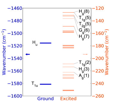
Figure 1: Low-energy vibronic levels mainly originating from the lowest JT states. Left column shows the lowest JT levels without excitation of the IR modes. The right column shows the vibronic levels with one vibrational excitation of the IR modes.

The vibronic states were numerically derived (Appendix B.2). The obtained low-energy vibronic levels are shown in Fig. 1 (see also Fig. S3 SM ). The lowest $T_{1u}$ and $H_{u}$ JT levels are not affected by $\hat{H}_{\text{vibro}}^{(2)}$, and thus, they are continued to be called JT states (left column in Fig. 1) The excited vibronic states arising from the $T_{1u}$ and $H_{u}$ JT states (right column in Fig. 1) are in a good approximation described by the symmetrized products of $T_{1u}/H_{u}$ JT states and $|\bm{n}^{\prime}\rangle$ involving only one IR vibrational excitation (see Appendix C and Table S5 SM ).

(a)	(b)	(c)	(d)

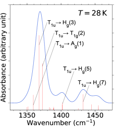
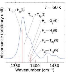
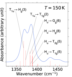
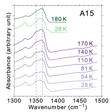
Figure 2: (a)-(c) Theoretical and (d) experimental IR spectra of A15 Cs₃C₆₀. Calculated IR spectra of C${}_{60}^{3-}$ at (a) 28 K, (b) 60 K, and (c) 150 K. All intensities (red vertical lines) are integrated with a Gauss function of full width of half maxima = 14 $\mathrm{cm^{-1}}$ (blue). In (d), the upper two (green) and lower six (purple) spectra are taken from Ref. Klupp et al. (2012) and Ref.Kamarás et al. (2013), respectively. The vertical dashed lines at 1350 and 1365 cm^-1 show the positions of the peaks of our interest.

V Vibronic excitations in infrared spectra

The IR absorption corresponds to the transition from the JT to the excited vibronic states (left and right columns of Fig. 1, respectively). Introducing the coupling to the external electric field $\bm{E}$ Bersuker and Polinger (1989); Kaplan and Vekhter (1995),

$$\hat{H}_{\text{IR}}=\sum_{\mu}\sum_{\gamma=x,y,z}Z_{\mu}\hat{q}_{t_{1u}(\mu)\gamma}E_{\gamma},$$ (6)

where $Z_{\mu}$ is effective nuclear charge, the IR absorbance is given by Sakurai (1994):

$$I(\omega,T) \propto \sum_{\kappa\tau\gamma}\rho_{\kappa}(T)\omega\left|\langle\Psi_{\tau}|\hat{q}_{t_{1u}(4)\gamma}|\Psi_{\kappa}\rangle\right|^{2}\delta\left(\omega-\omega_{\tau\kappa}\right),$$ (7)

where, $\kappa$ indicates the low-lying JT states, $\tau$ denotes the vibronic states with one IR excitation, $\rho_{\kappa}(T)$ is the canonical distribution at temperature $T$, and $\hslash\omega_{\tau\kappa}=E_{\tau}-E_{\kappa}$.

The simulated IR spectra of C${}_{60}^{3-}$ at (a) 28 K, (b) 60 K, and (c) 150 K are shown in Fig. 2. At 28 K, all the peaks are mainly composed of the excitations from the lowest $T_{1u}$ JT level. The highest peak around 1370 cm^-1 includes three major components corresponding to the excitations from the $T_{1u}$ to $H_{g}(3)$, $T_{1g}(2)$, and $A_{g}(1)$ vibronic levels (Fig. 1 and Table S6 SM ). In these IR-admixed vibronic states, the products of the $T_{1u}$ JT state and one $t_{1u}(4)$ vibrational excitation have large weight (Table S5 SM ). As temperature rises, the first excited $H_{u}$ JT state is also thermally populated, and thus, the fraction of the transitions from the $T_{1u}$ ($H_{u}$) JT state decreases (increases). The new peaks observed at high temperature correspond to the transitions from the $H_{u}$ to the $G_{g}(6)$, $H_{g}(8)$, $T_{2g}(5)$ and $T_{1g}(5)$ vibronic levels (Fig. 1 and Table S6 SM ) which mainly originate from the products of the $H_{u}$ JT state and one $t_{1u}(4)$ excitation (Table S5 SM ). The contributions from the $H_{u}$ are not negligible already at 60 K and eventually become stronger at high temperature [Fig. 2 (b), (c)] . The evolution explains the basic features of the experimental data: in the spectra, the peak around 1350 cm^-1 from the $T_{1u}$ JT level is the highest at $T=28$ K, while the peak at 1365 cm^-1 from the $H_{u}$ JT level becomes higher as temperature increases [Fig. 2 (d)] . Thus, the present theory proves that the temperature dependence indeed originates from thermal population of vibronic excitation from the $T_{1u}$ to the $H_{u}$ JT states. Besides the main peaks, some of the other fine structures can be explained. For example, the gradual decrease of the peak at 1400 cm^-1 [$T_{1u}\rightarrow H_{g}(5)$] with the increase of temperature resembles the temperature dependence of the shoulder at 1380 cm^-1 in the experimental data [Fig. 2 (d)]. Note that such small structures arises due to the quadratic vibronic coupling involving IR inactive $g_{u}/h_{u}$ modes besides IR active $t_{1u}$.

VI Discussion

The interpretation of the IR spectra of JT systems is often based on the modification of selection rules due to the symmetry lowering Thorson (1958). Thus, in the previous quantum chemistry study of Cs₃C₆₀ cluster, the IR spectra were calculated for some electronic configurations at statically deformed structure Naghavi et al. (2016). Considering the complicated orbital-lattice entangled nature of vibronic states, such simplified treatment is not sufficient to reveal the mechanisms of the implication of dynamical JT effect in the observed properties. The theoretical framework for a complete treatment of the JT dynamics and IR spectra in high symmetric JT systems is established in this work. On this basis, it is shown that the assumption of a change of adiabatic potential energy surface by thermal expansion Klupp et al. (2012); Kamarás et al. (2013) is not necessary for the description of the temperature evolution of IR spectra.

The obtained results can be applied to the analysis of the IR spectra in fullerides close to Mott transition where the IR spectra are practically unaffected by weak intersite interactions. In the metallic phase, the electron transfer interaction $\hat{H}_{\text{t}}$ is not negligible. In the ground state, $\hat{H}_{\text{t}}$ forms continuous vibronic states without quenching the JT dynamics because of the large stabilization energy of the latter Iwahara and Chibotaru (2015). As a consequence, the spin gap induced by the JT dynamics is observed even in the fullerides with small lattice constant Brouet et al. (2002). The IR-admixed vibronic states (right column of Fig. 1) are also mixed with many excited vibronic states involving one IR vibrational excitation by $\hat{H}_{\text{t}}$. At a sufficiently strong interaction of the excited vibronic states with a continuum of bulk states, a Fano resonance in IR spectra will appear. We stress that the modification of the shape of IR spectra into a Fano resonance Zadik et al. (2015) does not necessarily mean the quench of JT effect in the ground state.

The present work can also contribute to the description of the light-induced superconductivity in K₃C₆₀ Mitrano et al. (2016); Cantaluppi et al. (2018). The model used in recent works Kennes et al. (2017); Sentef (2017) for the discussion of possible mechanism based on a simplified quadratic vibronic coupling, should be replaced with Eq. (2). In Ref. Mitrano et al. (2016), the importance of the cubic coupling was also proposed to relate the vibration of IR active $t_{1u}$ mode and JT distortion, while it was shown here that these lattice degrees of freedom are already entangled (5) within the quadratic vibronic model via degenerate electronic terms.

VII Conclusion

The quantum mechanical framework for the description of the IR spectra of dynamical JT system is developed. Based on the first-principles calculations, the nonlinear vibronic Hamiltonian of C${}_{60}^{3-}$ site was derived, and the vibronic states involving both the JT and IR degrees of freedom were calculated. On this basis, the relation between the temperature evolution of IR spectra in Mott insulating Cs₃C₆₀ and JT dynamics was established. The first-principles calculations also showed non-negligible nonlinear vibronic couplings between the IR active $t_{1u}$ mode and non-IR active $g_{u}$ and $h_{u}$ modes, giving rise to the fine structures of the IR spectra. It is worthy to note that, contrary to the previous approaches, static JT distortions are not assumed to be responsible for the temperature evolution of IR spectra as well as their fine structure. Because the fine structure of the IR spectra is governed by the IR-admixed vibronic structure, the reconsideration on the relation between the IR spectra in metallic fullerides and the nature of JT dynamics as function of their volume is required. The developed theoretical approach can be applied to the study of the spectroscopic and light-induced electronic properties of various correlated dynamical JT materials.

Appendix A Quadratic vibronic coupling

In this section, SO(3) symmetry and the spherical basis for the $t_{1u}$ and $h_{u/g}$ irreps. of $I_{h}$ group are used. The Condon-Shortley’s phase convention is taken for the spherical harmonics Varshalovich et al. (1988).

A.1 Derivation of Eq. (3)

The $t_{1u}$ LUMOs couple to the symmetrized $h_{g}$ polynomials of the normal coordinates. The quadratic $h_{g}$ polynomials are calculated as

$$\{\hat{q}_{\Gamma_{1}(\mu_{1})}\otimes\hat{q}_{\Gamma_{2}(\mu_{2})}\}_{\nu h_{g}\gamma} = \sum_{\gamma_{1}\gamma_{2}}\langle\nu h_{g}\gamma|\Gamma_{1}\gamma_{1}\Gamma_{2}\gamma_{2}\rangle$$ (8)

$$\times \hat{q}_{\Gamma_{1}(\mu_{1})\gamma_{1}}\hat{q}_{\Gamma_{2}(\mu_{2})\gamma_{2}},$$

where the sum is over the components of the irreps. $\Gamma_{1}$ and $\Gamma_{2}$. See for the explicit form Sec. II in Ref. SM . The quadratic vibronic coupling is expressed as

$$\hat{H}_{\text{vibro}}^{(2)} = \sum_{\mu_{i}\Gamma_{i}}\sum_{\nu\gamma}\sum_{\lambda\lambda^{\prime}\sigma}V_{\nu\mu_{1}\mu_{2}}^{\Gamma_{1}\Gamma_{2}}\{\hat{q}_{\Gamma_{1}(\mu_{1})}\otimes\hat{q}_{\Gamma_{2}(\mu_{2})}\}_{\nu h_{g}\gamma}$$ (9)

$$\times \sqrt{\frac{5}{2}}\langle t_{1u}\lambda|t_{1u}\lambda^{\prime},h_{g}\gamma\rangle\hat{c}_{t_{1u}\lambda\sigma}^{\dagger}\hat{c}_{t_{1u}\lambda^{\prime}\sigma},$$

where $\sigma$ indicates the projection of electron spin and $\hat{c}_{t_{1u}\lambda\sigma}^{\dagger}$ and $\hat{c}_{t_{1u}\lambda\sigma}$ are the electron creation and annihilation operators in spin-orbital $t_{1u}\lambda\sigma$. Transforming the real components of the irreps. into the spherical ones, Eq. (9) reduces to the same form as Eq. (A1) in Ref. Liu et al. (2018a). Thus, by the same procedure as described in the Appendix A in Ref. Liu et al. (2018a), we obtain the spherical form of Eq. (3):

$$\hat{H}^{(2)}_{\text{vibro}} = \sum_{\mu_{i}\Gamma_{i}}\sum_{\nu m^{\prime\prime}}\sum_{nn^{\prime}}(-1)^{m^{\prime\prime}}V^{\Gamma_{1}\Gamma_{2}}_{\nu\mu_{1}\mu_{2}}$$ (10)

$$\times \{\hat{q}_{\Gamma_{1}(\mu_{1})}\otimes\hat{q}_{\Gamma_{2}(\mu_{2})}\}_{\nu 2,-m^{\prime\prime}}\sqrt{\frac{15}{2}}\langle 1n|2n^{\prime},2m^{\prime\prime}\rangle$$

$$\times \left[|1n\rangle\langle 2n^{\prime}|-(-1)^{m^{\prime\prime}}|2,-n^{\prime}\rangle\langle 1,-n|\right],$$

where, $|1n\rangle$ and $|2n^{\prime}\rangle$ express the spherical form of the $T_{1u}$ and $H_{u}$ multiplet states, respectively, and $n,n^{\prime},m^{\prime\prime}$ the projections of the angular momenta. By the inverse transformation from the spherical into the Cartesian basis, we obtain Eq. (3). The difference in the coefficients in Eqs. (3), (10) and Eq. (9) by $\sqrt{3}$ comes from the reduced matrix element of Racah’s $\hat{U}^{(2)}$ operator. Since the spin and orbital degrees of freedom are independent from each other, Eqs. (3) and (10) show only the orbital part.

A.2 Model Hamiltonian for the IR modes

One-electron quadratic vibronic Hamiltonian for the IR modes is given by

$$\hat{H}_{0}^{\prime}+\hat{H}_{\text{vibro}}^{(2)\prime} = \left(|t_{1u}x\rangle,|t_{1u}y\rangle,|t_{1u}z\rangle\right)$$ (11)

$$\times \left(\mathbf{H}_{0}^{\prime}+\mathbf{H}^{(2)\prime}_{\text{vibro}}\right)\begin{pmatrix}\langle t_{1u}x|\\ \langle t_{1u}y|\\ \langle t_{1u}z|\end{pmatrix}.$$

Here, the projection of the electron spin is omitted, $\mathbf{H}_{0}^{\prime}$ involves the orbital energy $\epsilon_{t_{1u}}$ and the harmonic oscillator terms, and $\mathbf{H}^{(2)\prime}_{\text{vibro}}$ is the quadratic vibronic coupling:

$$\mathbf{H}_{0}^{\prime} = \left(\epsilon_{t_{1u}}+\sum_{\gamma=x,y,z}\frac{k_{t_{1u}(4)}}{2}q_{t_{1u}(4)\gamma}^{2}+\sum_{\gamma=a,x,y,z}\frac{k_{g_{u}(5)}}{2}q_{g_{u}(5)\gamma}^{2}+\sum_{\gamma=\theta,\epsilon,\xi,\eta,\zeta}\frac{k_{h_{u}(6)}}{2}q_{h_{u}(6)\gamma}^{2}\right)\mathbf{I},$$ (12)

$$\mathbf{H}^{(2)\prime}_{\text{vibro}} = \sum_{\gamma=\theta,\epsilon,\xi,\eta,\zeta}\left(V^{t_{1u}t_{1u}}_{44}\{\hat{q}_{t_{1u}(4)}\otimes\hat{q}_{t_{1u}(4)}\}_{h_{g}\gamma}+V^{g_{u}g_{u}}_{55}\{\hat{q}_{g_{u}(5)}\otimes\hat{q}_{g_{u}(5)}\}_{h_{g}\gamma}+\sum_{\nu=1,2}V^{h_{u}h_{u}}_{\nu 66}\{\hat{q}_{h_{u}(6)}\otimes\hat{q}_{h_{u}(6)}\}_{\nu h_{g}\gamma}\right.$$ (13)

$$+ \left.2V^{t_{1u}g_{u}}_{45}\{\hat{q}_{t_{1u}(4)}\otimes\hat{q}_{g_{u}(5)}\}_{h_{g}\gamma}+2V^{t_{1u}h_{u}}_{46}\{\hat{q}_{t_{1u}(4)}\otimes\hat{q}_{h_{u}(6)}\}_{h_{g}\gamma}+\sum_{\nu=1,2}2V^{g_{u}h_{u}}_{\nu 56}\{\hat{q}_{g_{u}(5)}\otimes\hat{q}_{h_{u}(6)}\}_{\nu h_{g}\gamma}\right)\mathbf{M}_{\gamma},$$

$k_{\Gamma(\mu)}$ indicates the elastic parameter, $\mathbf{I}$ is the three-dimensional unit matrix, and

$$\mathbf{M}_{\theta} = \begin{pmatrix}\frac{1}{2}&0&0\\ 0&\frac{1}{2}&0\\ 0&0&-1\\ \end{pmatrix},\quad\mathbf{M}_{\epsilon}=\begin{pmatrix}-\frac{\sqrt{3}}{2}&0&0\\ 0&\frac{\sqrt{3}}{2}&0\\ 0&0&0\\ \end{pmatrix},$$

$$\mathbf{M}_{\xi} = \begin{pmatrix}0&0&0\\ 0&0&-\frac{\sqrt{3}}{2}\\ 0&-\frac{\sqrt{3}}{2}&0\\ \end{pmatrix},\quad\mathbf{M}_{\eta}=\begin{pmatrix}0&0&-\frac{\sqrt{3}}{2}\\ 0&0&0\\ -\frac{\sqrt{3}}{2}&0&0\\ \end{pmatrix},$$

$$\mathbf{M}_{\zeta} = \begin{pmatrix}0&-\frac{\sqrt{3}}{2}&0\\ -\frac{\sqrt{3}}{2}&0&0\\ 0&0&0\\ \end{pmatrix}.$$ (14)

In Eqs. (12) and (13), only the IR modes Note (5) are included.

A.3 Derivation of Eq. (4)

The transformation from Eq. (3) to Eq. (4) is described here. In this subsection, to make use of the SO(3) symmetry of the linear $t_{1u}^{3}\otimes h_{g}$ JT system, the vibronic angular momentum $J$ is used instead of real irrep $\Gamma$ of $I_{h}$ group.

Using the identity operator for the JT states, $\hat{I}^{(0)}=\sum_{\alpha JmP}|\Phi^{(0)}_{\alpha JmP}\rangle\langle\Phi^{(0)}_{\alpha JmP}|$,

$$\hat{H}_{\text{vibro}}^{(2)} = \hat{I}^{(0)}\hat{H}_{\text{vibro}}^{(2)}\hat{I}^{(0)}$$ (15)

$$= \sum_{\alpha JmP}\sum_{\alpha^{\prime}J^{\prime}m^{\prime}P^{\prime}}\langle\Psi^{(0)}_{\alpha JmP}|\hat{H}_{\text{vibro}}^{(2)}|\Psi^{(0)}_{\alpha^{\prime}J^{\prime}m^{\prime}P^{\prime}}\rangle$$

$$\times |\Psi^{(0)}_{\alpha JmP}\rangle\langle\Psi^{(0)}_{\alpha^{\prime}J^{\prime}m^{\prime}P^{\prime}}|,$$

where, $J$ is the vibronic angular momentum and $m$ is its projection. Substituting Eq. (10) into the matrix element of Eq. (15), we obtain

$$\hat{H}_{\text{vibro}}^{(2)} = \sum_{\alpha JmP}\sum_{\alpha^{\prime}J^{\prime}m^{\prime}P^{\prime}}\sum_{\mu_{i}\Gamma_{i}}\sum_{\nu m^{\prime\prime}}V^{\Gamma_{1}\Gamma_{2}}_{\nu\mu_{1}\mu_{2}}$$

$$\times (-1)^{m^{\prime\prime}}\{\hat{q}_{\Gamma_{1}(\mu_{1})}\otimes\hat{q}_{\Gamma_{2}(\mu_{2})}\}_{\nu 2,-m^{\prime\prime}}\sqrt{\frac{15}{2}}$$

$$\times \langle\Psi^{(0)}_{\alpha JmP}|\hat{M}_{2m^{\prime\prime}}|\Psi^{(0)}_{\alpha^{\prime}J^{\prime}m^{\prime}P^{\prime}}\rangle|\Psi^{(0)}_{\alpha JmP}\rangle\langle\Psi^{(0)}_{\alpha^{\prime}J^{\prime}m^{\prime}P^{\prime}}|,$$

with rank 2 irreducible tensor operator

$$\hat{M}_{2m^{\prime\prime}} = \sum_{nn^{\prime}}\langle 1n|2n^{\prime},2m^{\prime\prime}\rangle$$ (17)

$$\times \left[|1n\rangle\langle 2n^{\prime}|-(-1)^{m^{\prime\prime}}|2,-n^{\prime}\rangle\langle 1,-n|\right].$$

Applying Wigner-Eckart theorem Varshalovich et al. (1988) to the matrix elements of $\hat{M}_{2m^{\prime\prime}}$,

$$\langle\Psi^{(0)}_{\alpha Jm+}| \hat{M}_{2m^{\prime\prime}}|\Psi^{(0)}_{\alpha^{\prime}J^{\prime}m^{\prime}-}\rangle$$ (18)

$$=\frac{\langle\Psi^{(0)}_{\alpha J+}\|\hat{M}_{2}\|\Psi^{(0)}_{\alpha^{\prime}J^{\prime}-}\rangle}{\sqrt{2J+1}}\langle Jm|J^{\prime}m^{\prime},2m^{\prime\prime}\rangle$$

$$=\Xi(\alpha J+;\alpha^{\prime}J^{\prime}-)\langle Jm|J^{\prime}m^{\prime},2m^{\prime\prime}\rangle.$$

Here, the parities of the $T_{1u}$ and $H_{u}$ terms are defined to be $+1$ and $-1$, respectively [see Eq. (11) in Ref. Liu et al. (2018a)], and $\Xi(\alpha JP;\alpha^{\prime}J^{\prime}P^{\prime})$ is defined by

$$\Xi(\alpha JP;\alpha^{\prime}J^{\prime}P^{\prime}) = \frac{\langle\Psi^{(0)}_{\alpha JP}\|\hat{M}_{2}\|\Psi^{(0)}_{\alpha^{\prime}J^{\prime}P^{\prime}}\rangle}{\sqrt{2J+1}}.$$ (19)

Therefore, by the substitution of Eq. (18) into Eq. (LABEL:Eq:IHQI2), we obtain

$$\hat{H}_{\text{vibro}}^{(2)} = \sum_{\alpha Jm}\sum_{\alpha^{\prime}J^{\prime}m^{\prime}}\sum_{\mu_{i}\Gamma_{i}}\sum_{\nu m^{\prime\prime}}V^{\Gamma_{1}\Gamma_{2}}_{\nu\mu_{1}\mu_{2}}\Xi(\alpha J+;\alpha^{\prime}J^{\prime}-)$$ (20)

$$\times (-1)^{m^{\prime\prime}}\{\hat{q}_{\Gamma_{1}(\mu_{1})}\otimes\hat{q}_{\Gamma_{2}(\mu_{2})}\}_{\nu 2,-m^{\prime\prime}}\sqrt{\frac{15}{2}}$$

$$\times \langle Jm|J^{\prime}m^{\prime},2m^{\prime\prime}\rangle|\Psi^{(0)}_{\alpha Jm+}\rangle\langle\Psi^{(0)}_{\alpha^{\prime}J^{\prime}m^{\prime}-}|+\text{h.c.}$$

$$= \sum_{\alpha JmP}\sum_{\alpha^{\prime}J^{\prime}m^{\prime}P^{\prime}}\sum_{\mu_{i}\Gamma_{i}}\sum_{\nu m^{\prime\prime}}V^{\Gamma_{1}\Gamma_{2}}_{\nu\mu_{1}\mu_{2}}\Xi(\alpha JP;\alpha^{\prime}J^{\prime}P^{\prime})$$

$$\times (-1)^{m^{\prime\prime}}\{\hat{q}_{\Gamma_{1}(\mu_{1})}\otimes\hat{q}_{\Gamma_{2}(\mu_{2})}\}_{\nu 2,-m^{\prime\prime}}\sqrt{\frac{15}{2}}$$

$$\times \langle Jm|J^{\prime}m^{\prime},2m^{\prime\prime}\rangle|\Psi^{(0)}_{\alpha JmP}\rangle\langle\Psi^{(0)}_{\alpha^{\prime}J^{\prime}m^{\prime}P^{\prime}}|.$$

To obtain the second form,

$$\left[\{\hat{q}_{\Gamma_{1}(\mu_{1})}\right. \otimes\left.\hat{q}_{\Gamma_{2}(\mu_{2})}\}_{\nu 2,-m^{\prime\prime}}\right]^{\dagger}$$ (21)

$$=(-1)^{m^{\prime\prime}}\{\hat{q}_{\Gamma_{1}(\mu_{1})}\otimes\hat{q}_{\Gamma_{2}(\mu_{2})}\}_{\nu 2m^{\prime\prime}},$$

and

$$\Xi( \alpha J+;\alpha^{\prime}J^{\prime}-)\langle Jm|J^{\prime}m^{\prime},2m^{\prime\prime}\rangle$$ (22)

$$=\Xi(\alpha^{\prime}J^{\prime}-;\alpha J+)(-1)^{m^{\prime\prime}}\langle J^{\prime}m^{\prime}|Jm,2,-m^{\prime\prime}\rangle,$$

are used. Nonzero $\Xi(\alpha J+;\alpha^{\prime}J^{\prime}-)$’s for the low-energy JT levels are shown in Table S4 SM . Finally, using the relation between the irreps. of SO(3) and $I_{h}$ in Eq. (20), we obtain Eq. (4). For details of the relation of these two representations, see Sec. I A in the Supplemental Materials of Ref. Liu et al. (2018b).

Appendix B Computational methods

B.1 DFT calculations

In order to determine the frequencies and the quadratic vibronic coupling parameters, DFT calculations of Cs₃C₆₀ cluster were performed. The cluster con sits of one C₆₀, the nearest 12 Cs atoms and several thousands of point charges for distant C${}_{60}^{3-}$ ($-3$) and Cs⁺ ($+1$). For the calculations, B3LYP hybrid exchange-correlation functional was used with a triple-zeta polarization 6-311G(d) and double zeta 3-21G basis sets for C and Cs, respectively Frisch et al. . In order to avoid the artificial splitting of the $t_{1u}$ orbital levels, the ${}^{4}A_{u}$ electronic configuration was treated within spin-unrestricted approach. The quadratic vibronic coupling constants were derived by fitting the $t_{1u}$ LUMO levels with respect to the deformed structures to the model Hamiltonian, Eq. (11). The results of the fitting are shown in Fig. S2 SM .

B.2 Calculation of vibronic states

The vibronic Hamiltonian matrix was derived using the JT states of Ref. Liu et al. (2018a), and then numerically diagonalized . The basis of $|\Psi_{\tau}\rangle$ (5) was truncated on the basis of the excitation energy of JT states and the number of vibrational excitations for IR modes Note (5): the former was $<$ 90 meV and the latter was 3,

$$0\leq\sum_{\Gamma(\mu)\gamma}n^{\prime}_{\Gamma(\mu)\gamma}\leq 3,$$ (23)

where, the sum is over the IR modes, and $n^{\prime}_{\Gamma(\mu)\gamma}\geq 0$ is vibrational quantum number. The cutoff of the JT states restricts the maximum temperature for the simulation of the IR spectra as in the case of spin gap Liu et al. (2018a) because the JT levels higher than the cutoff cannot be populated. The maximum temperature treated in this work is 150 K.

Appendix C Assignment of the vibronic states

The lowest vibronic states (left column of Fig. 1) are expressed by the linear combinations of the products of the JT states and the vibrational vacuum $|\bm{n}^{\prime}=\bm{0}\rangle$ or two vibrationally excited states of the IR modes Note (5). The contribution from the latter is negligible in the present case, and thus, these low-energy vibronic states are well defined by the JT states.

On the other hand, the excited vibronic states (right column of Fig. 1) are described by the linear combination of the products of the JT states and the one- or three-vibrationally excited IR states, and the main contributions come from the former. Therefore, the excited vibronic states $|\Psi_{\tau}\rangle$ are assigned by the symmetrized products of the JT and the one vibrationally excited states. The symmetrized states are expressed as

$$|(\Gamma_{1}\Gamma_{2})n\Gamma\gamma\rangle = \sum_{\gamma_{1}\gamma_{2}}|\Gamma_{1}\gamma_{1}\rangle\otimes|\Gamma_{2}\gamma_{2}\rangle\langle\Gamma_{1}\gamma_{1},\Gamma_{2}\gamma_{2}|\nu\Gamma\gamma\rangle,$$

where, $\Gamma_{1}$ and $\Gamma_{2}$ indicate the irreps. of the JT and IR states, respectively. Thus, $\Gamma_{2}$ is the irrep of the excited IR mode. The product states of the $T_{1u}$ JT state and the $t_{1u}$, $g_{u}$, $h_{u}$ vibrational states split into 10 states,

$$T_{1u}\otimes t_{1u} = A_{g}\oplus T_{1g}\oplus H_{g},$$

$$T_{1u}\otimes g_{u} = T_{2g}\oplus G_{g}\oplus H_{g},$$

$$T_{1u}\otimes h_{u} = T_{1g}\oplus T_{2g}\oplus G_{g}\oplus H_{g},$$ (25)

and those with the $H_{u}$ JT state into 16 states,

$$H_{u}\otimes t_{1u} = T_{1g}\oplus T_{2g}\oplus G_{g}\oplus H_{g},$$

$$H_{u}\otimes g_{u} = T_{1g}\oplus T_{2g}\oplus G_{g}\oplus 2H_{g},$$

$$H_{u}\otimes h_{u} = A_{g}\oplus T_{1g}\oplus T_{2g}\oplus 2G_{g}\oplus 2H_{g},$$ (26)

respectively. The explicit forms of the symmetrized vibronic states (LABEL:Eq:symm) are given in Sec. IV A of Ref. SM . The contribution of each symmetrized state (LABEL:Eq:symm) to the vibronic states $|\Psi_{\tau}\rangle$, Eq. (5), is quantitatively evaluated by calculating

$$w(\Gamma_{1}\Gamma_{2}\nu\Gamma,\tau) = \langle\Psi_{\tau}|\hat{I}_{(\Gamma_{1}\Gamma_{2})\nu\Gamma}|\Psi_{\tau}\rangle,$$ (27)

where, $\hat{I}_{(\Gamma_{1}\Gamma_{2})\nu\Gamma}$ is the projector into the symmetrized states $(\Gamma_{1}\Gamma_{2})\nu\Gamma\gamma$,

$$\hat{I}_{(\Gamma_{1}\Gamma_{2})\nu\Gamma} = \sum_{\gamma}|(\Gamma_{1}\Gamma_{2})\nu\Gamma\gamma\rangle\langle(\Gamma_{1}\Gamma_{2})\nu\Gamma\gamma|.$$ (28)

Eq. (27) also enables us to skip the analysis of the structure of $|\Psi_{\tau}\rangle$ for the assignment. The list of $w(\Gamma_{1}\Gamma_{2}\nu\Gamma,\tau)$ are given in Table S5 SM .

References

- Bersuker and Polinger (1989) I. B. Bersuker and V. Z. Polinger, Vibronic Interactions in Molecules and Crystals (Springer–Verlag, Berlin, 1989).
- Kaplan and Vekhter (1995) M. D. Kaplan and B. G. Vekhter, Cooperative Phenomena in Jahn-Teller Crystals (Plenum Press, New York and London, 1995).
- Chancey and O’Brien (1997) C. C. Chancey and M. C. M. O’Brien, The Jahn–Teller Effect in C60 and Other Icosahedral Complexes (Princeton University Press, Princeton, 1997).
- Krimmel et al. (2005) A. Krimmel, M. Mücksch, V. Tsurkan, M. M. Koza, H. Mutka, and A. Loidl, “Vibronic and Magnetic Excitations in the Spin-Orbital Liquid State of ,” Phys. Rev. Lett. 94, 237402 (2005).
- de Vries et al. (2010) M. A. de Vries, A. C. Mclaughlin, and J.-W. G. Bos, “Valence Bond Glass on an fcc Lattice in the Double Perovskite ,” Phys. Rev. Lett. 104, 177202 (2010).
- Nakatsuji et al. (2012) S. Nakatsuji, K. Kuga, K. Kimura, R. Satake, N. Katayama, E. Nishibori, H. Sawa, R. Ishii, M. Hagiwara, F. Bridges, T. U. Ito, W. Higemoto, Y. Karaki, M. Halim, A. A. Nugroho, J. A. Rodriguez-Rivera, M. A. Green, and C. Broholm, “Spin-orbital short-range order on a honeycomb-based lattice,” Science 336, 559 (2012).
- Kamazawa et al. (2017) K. Kamazawa, M. Ishikado, S. Ohira-Kawamura, Y. Kawakita, K. Kakurai, K. Nakajima, and M. Sato, “Interaction of spin-orbital-lattice degrees of freedom: Vibronic state of the corner-sharing-tetrahedral frustrated spin system by dynamical Jahn-Teller effect,” Phys. Rev. B 95, 104413 (2017).
- Nirmala et al. (2017) R. Nirmala, K.-H. Jang, H. Sim, H. Cho, J. Lee, N.-G. Yang, S. Lee, R. M. Ibberson, K. Kakurai, M. Matsuda, S.-W. Cheong, V. V. Gapontsev, S. V. Streltsov, and J.-G. Park, “Spin glass behavior in frustrated quantum spin system CuAl2O4 with a possible orbital liquid state,” J. Phys. Condens. Matter 29, 13LT01 (2017).
- Webster et al. (2007) C. H. Webster, L. M. Helme, A. T. Boothroyd, D. F. McMorrow, S. B. Wilkins, C. Detlefs, B. Detlefs, R. I. Bewley, and M. J. McKelvy, “Influence of static Jahn-Teller distortion on the magnetic excitation spectrum of : A synchrotron x-ray and neutron inelastic scattering study,” Phys. Rev. B 76, 134419 (2007).
- Santini et al. (2009) P. Santini, S. Carretta, G. Amoretti, R. Caciuffo, N. Magnani, and G. H. Lander, “Multipolar interactions in -electron systems: The paradigm of actinide dioxides,” Rev. Mod. Phys. 81, 807 (2009).
- Yamaguchi et al. (1997) S. Yamaguchi, Y. Okimoto, and Y. Tokura, “Local lattice distortion during the spin-state transition in ,” Phys. Rev. B 55, R8666 (1997).
- Klupp et al. (2006) G. Klupp, K. Kamarás, N. M. Nemes, C. M. Brown, and J. Leão, “Static and dynamic Jahn-Teller effect in the alkali metal fulleride salts ,” Phys. Rev. B 73, 085415 (2006).
- Jung et al. (2008) S.-H. Jung, J.-H. Noh, J. Kim, C. L. Zhang, S. W. Cheong, and E. J. Choi, “Infrared phonon study of the spinel oxide ZnV2O4,” J. Phys. Condens. Matter 20, 175205 (2008).
- Francis et al. (2012) E. A. Francis, S. Scharinger, K. Németh, K. Kamarás, and C. A. Kuntscher, “Pressure-induced transition from the dynamic to static Jahn-Teller effect in (Ph4P)2IC60,” Phys. Rev. B 85, 195428 (2012).
- Klupp et al. (2012) G. Klupp, P. Matus, K. Kamarás, A. Y. Ganin, A. McLennan, M. J. Rosseinsky, Y. Takabayashi, M. T. McDonald, and K. Prassides, “Dynamic Jahn-Teller effect in the parent insulating state of the molecular superconductor Cs3C60,” Nat. Commun. 3, 912 (2012).
- Kamarás et al. (2013) K. Kamarás, G. Klupp, P. Matus, A. Y. Ganin, A. McLennan, M. J. Rosseinsky, Y. Takabayashi, M. T. McDonald, and K. Prassides, “Mott localization in the correlated superconductor Cs3C60 resulting from the molecular Jahn-Teller effect,” J. Phys.: Conf. Ser. 428, 012002 (2013).
- Qu et al. (2013) Z. Qu, Y. Zou, S. Zhang, L. Ling, L. Zhang, and Y. Zhang, “Spin-phonon coupling probed by infrared transmission spectroscopy in the double perovskite Ba2YMoO6,” J. Appl. Phys. 113, 17E137 (2013).
- Zadik et al. (2015) R. H. Zadik, Y. Takabayashi, G. Klupp, R. H. Colman, A. Y. Ganin, A. Potočnik, P. Jeglič, D. Arčon, P. Matus, K. Kamarás, Y. Kasahara, Y. Iwasa, A. N. Fitch, Y. Ohishi, G. Garbarino, K. Kato, M. J. Rosseinsky, and K. Prassides, “Optimized unconventional superconductivity in a molecular Jahn-Teller metal,” Sci. Adv. 1, e1500059 (2015).
- Constable et al. (2017) E. Constable, R. Ballou, J. Robert, C. Decorse, J.-B. Brubach, P. Roy, E. Lhotel, L. Del-Rey, V. Simonet, S. Petit, and S. deBrion, “Double vibronic process in the quantum spin ice candidate revealed by terahertz spectroscopy,” Phys. Rev. B 95, 020415 (2017).
- Lavrentiev et al. (2017) V. Lavrentiev, D. Chvostova, I. Lavrentieva, J. Vacik, Y. Daskal, M. Barchuk, D. Rafaja, and A. Dejneka, “Optical transitions and electronic interactions in self-assembled cobalt-fullerene mixture films,” J. Phys. D: Appl. Phys. 50, 485305 (2017).
- Gunnarsson (1997) O. Gunnarsson, “Superconductivity in fullerides,” Rev. Mod. Phys. 69, 575 (1997).
- Gunnarsson (2004) O. Gunnarsson, Alkali-Doped Fullerides: Narrow-Band Solids with Unusual Properties (World Scientific, Singapore, 2004).
- Auerbach et al. (1994) A. Auerbach, N. Manini, and E. Tosatti, “Electron-vibron interactions in charged fullerenes. I. Berry phases,” Phys. Rev. B 49, 12998 (1994).
- Manini et al. (1994) N. Manini, E. Tosatti, and A. Auerbach, “Electron-vibron interactions in charged fullerenes. II. Pair energies and spectra,” Phys. Rev. B 49, 13008 (1994).
- O’Brien (1996) M. C. M. O’Brien, “Vibronic energies in and the Jahn-Teller effect,” Phys. Rev. B 53, 3775 (1996).
- Chibotaru (2005) L. F. Chibotaru, “Spin-Vibronic Superexchange in Mott-Hubbard Fullerides,” Phys. Rev. Lett. 94, 186405 (2005).
- Nomura et al. (2016) Y. Nomura, S. Sakai, M. Capone, and R. Arita, “Exotic -wave superconductivity in alkali-doped fullerides,” J. Phys.: Condens. Matter 28, 153001 (2016).
- Nava et al. (2018) A. Nava, C. Giannetti, A. Georges, E. Tosatti, and M. Fabrizio, “Cooling quasiparticles in A3C60 fullerides by excitonic mid-infrared absorption,” Nat. Phys. 14, 154 (2018).
- Iwahara (2018) N. Iwahara, “Berry phase of adiabatic electronic configurations in fullerene anions,” Phys. Rev. B 97, 075413 (2018).
- Iwahara et al. (2010) N. Iwahara, T. Sato, K. Tanaka, and L. F. Chibotaru, “Vibronic coupling in anion revisited: Derivations from photoelectron spectra and DFT calculations,” Phys. Rev. B 82, 245409 (2010).
- Iwahara and Chibotaru (2013) N. Iwahara and L. F. Chibotaru, “Dynamical Jahn-Teller Effect and Antiferromagnetism in Cs3C60,” Phys. Rev. Lett. 111, 056401 (2013).
- Liu et al. (2018a) D. Liu, N. Iwahara, and L. F. Chibotaru, “Dynamical Jahn-Teller effect of fullerene anions,” Phys. Rev. B 97, 115412 (2018a).
- Judd (1974) B. R. Judd, “Lie Groups and the Jahn-Teller Effect,” Can. J. Phys. 52, 999 (1974).
- Chibotaru and Kotov (1994) L.F. Chibotaru and I.N. Kotov, “Polaron-like variational solutions for low-lying vibronic states,” Chem. Phys. 185, 153 (1994).
- Iwahara and Chibotaru (2015) N. Iwahara and L. F. Chibotaru, “Dynamical Jahn-Teller instability in metallic fullerides,” Phys. Rev. B 91, 035109 (2015).
- Iwahara and Chibotaru (2016) N. Iwahara and L. F. Chibotaru, “Orbital disproportionation of electronic density is a universal feature of alkali-doped fullerides,” Nat. Commun. 7, 13093 (2016).
- Note (1) In the inequivalent subbands, the electron correlation develops in different ways. The evolution of the electron correlation can be seen in the Gutzwiller’s reduction factors with respect to Coulomb repulsion on C60 sites (see Fig. 2d in Ref. Iwahara and Chibotaru (2016)). As the increase of the Coulomb repulsion on C60 sites the Gutzwiller’s factor of half-filled subband becomes close to zero (strongly correlated), whereas those for empty and filled subbands become close to one (uncorrelated). Since the metallic screening and the band energy for nondegenerate system are smaller than those of degenerate band, the critical Coulomb repulsion on C60 sites for the Mott transition is smaller too (Sec. VI in Ref. Iwahara and Chibotaru (2015)).
- (38) Y. Matsuda, S. Heguri, and K. Tanigaki, in preparation.
- Brouet et al. (2002) V. Brouet, H. Alloul, S. Garaj, and L. Forró, “Persistence of molecular excitations in metallic fullerides and their role in a possible metal to insulator transition at high temperatures,” Phys. Rev. B 66, 155124 (2002).
- Jeglič et al. (2009) P. Jeglič, D. Arčon, A. Potočnik, A. Y. Ganin, Y. Takabayashi, M. J. Rosseinsky, and K. Prassides, “Low-moment antiferromagnetic ordering in triply charged cubic fullerides close to the metal-insulator transition,” Phys. Rev. B 80, 195424 (2009).
- Note (2) The calculations in Ref. Iwahara and Chibotaru (2015) show unquenched dynamical JT effect on the C sites in Cs3C60 which is gradually quenched approaching the limit of JT glass in fullerides of a smaller volume like K3C60. The observed transformation of the shape of the IR line can be related to this change of the character of JT effect but not to its full disappearance as was supposed in Ref. Zadik et al. (2015). See also Sec. VI.
- Alloul et al. (2017) H. Alloul, P. Wzietek, T. Mito, D. Pontiroli, M. Aramini, M. Riccò, J. P. Itie, and E. Elkaim, “Mott Transition in the Phase of : Absence of a Pseudogap and Charge Order,” Phys. Rev. Lett. 118, 237601 (2017).
- (43) See Supplemental Materials at http://link.aps.org/supplemental/10.1103/PhysRevB.98.165410 for the definition of normal modes, symmetrized quadratic polynomials of coordinates, DFT data, assignment of the vibronic states and transition dipole intensities.
- Nomura et al. (2012) Y. Nomura, K. Nakamura, and R. Arita, “Ab initio derivation of electronic low-energy models for c60 and aromatic compounds,” Phys. Rev. B 85, 155452 (2012).
- Note (3) Displacement of nuclei along () direction from a high-symmetric reference structure is expressed by mass-weighted coordinates as , where is the mass of nucleus , and is the polarization vector of normal mode. The polarization vector is dimensionless, and the dimension of is , where is mass of electron and is Bohr radius. See for detail Sec. 10.1 in Ref. Inui et al. (1990).
- Racah (1943) G. Racah, “Theory of Complex Spectra. III,” Phys. Rev. 63, 367 (1943).
- Liu et al. (2018b) D. Liu, Y. Niwa, N. Iwahara, T. Sato, and L. F. Chibotaru, “Quadratic Jahn-Teller effect of fullerene anions,” Phys. Rev. B 98, 035402 (2018b).
- Note (4) The orders of the obtained quadratic coupling parameters and the expectation value of the product of IR coordinates are a.u. and a.u., respectively, therefore, the energy scale of each quadratic vibronic coupling is - a.u. Here, is approximated as using the harmonic oscillator model with cm-1 and the averaged vibrational quantum number 0-1. On the other hand, the energy scale of the linear vibronic coupling is a.u. in terms of the JT energy for C.
- Note (5) Both the IR active and inactive and modes are called IR modes because these three modes are admixed by the quadratic vibronic coupling, resulting in the contribution to the fine structure of the IR spectrum.
- Note (6) In this work, we treat two types of vibronic states. The first ones are the eigenstates of linear JT Hamiltonian and the second are eigenstates of the full Hamiltonian , including nonlinear vibronic couplings to the IR modes. To avoid the confusion, we call the former JT states and the latter vibronic states.
- Sakurai (1994) J. J. Sakurai, Modern quantum mechanics (revised edition) (Addison-Wesley, Boston, 1994).
- Note (7) At higher temperature above 150 K, many peaks from these excited JT levels above the and ones and the broadening of the line width smear the shape of the fine structures of the IR spectrum.
- Note (8) The slight difference between the theoretical and experimental shapes of the main peaks might be explained by the small shift of the theoretical vibronic levels from the real ones due to e.g. the absence of weak intersite interactions and crystal field effect in our calculations or the imperfect agreement between the DFT and experimental parameters. One also should note the sample dependence of IR spectra: Although both experimental data show the growth of new peak as the rise of temperature, the main peaks at 28 K at the bottom and the top of Fig. 2 (d) have slightly different fine structures.
- Thorson (1958) W. R. Thorson, “Vibronically Induced Absorption of Forbidden Infrared Transitions,” J. Chem. Phys. 29, 938 (1958).
- Naghavi et al. (2016) S. S. Naghavi, M. Fabrizio, T. Qin, and E. Tosatti, “Nanoscale orbital excitations and the infrared spectrum of a molecular Mott insulator: A15-Cs3C60,” Nanoscale 8, 17483 (2016).
- Mitrano et al. (2016) M. Mitrano, A. Cantaluppi, D. Nicoletti, S. Kaiser, A. Perucchi, S. Lupi, P. Di Pietro, D. Pontiroli, M. Riccó, S. R. Clark, D. Jaksch, and A. Cavalleri, “Possible light-induced superconductivity in K3C60 at high temperature,” Nature 530, 461 (2016).
- Cantaluppi et al. (2018) A. Cantaluppi, M. Buzzi, G. Jotzu, D. Nicoletti, M. Mitrano, D. Pontiroli, M. Riccó, A. Perucchi, P. Di Pietro, and A. Cavalleri, “Pressure tuning of light-induced superconductivity in K3C60,” Nat. Phys. 14, 837 (2018).
- Kennes et al. (2017) D. M. Kennes, E. Y. Wilner, D. R. Reichman, and A. J. Millis, “Transient superconductivity from electronic squeezing of optically pumped phonons,” Nat. Phys. 13, 479 (2017).
- Sentef (2017) M. A. Sentef, “Light-enhanced electron-phonon coupling from nonlinear electron-phonon coupling,” Phys. Rev. B 95, 205111 (2017).
- Varshalovich et al. (1988) D. A. Varshalovich, A. N. Moskalev, and V. K. Khersonskii, Quantum Theory of Angular Momentum (World Scientific, Singapore, 1988).
- (61) M. J. Frisch, G. W. Trucks, H. B. Schlegel, G. E. Scuseria, M. A. Robb, J. R. Cheeseman, G. Scalmani, V. Barone, B. Mennucci, G. A. Petersson, H. Nakatsuji, M. Caricato, X. Li, H. P. Hratchian, A. F. Izmaylov, J. Bloino, G. Zheng, J. L. Sonnenberg, M. Hada, M. Ehara, K. Toyota, R. Fukuda, J. Hasegawa, M. Ishida, T. Nakajima, Y. Honda, O. Kitao, H. Nakai, T. Vreven, J. A. Montgomery, Jr., J. E. Peralta, F. Ogliaro, M. Bearpark, J. J. Heyd, E. Brothers, K. N. Kudin, V. N. Staroverov, R. Kobayashi, J. Normand, K. Raghavachari, A. Rendell, J. C. Burant, S. S. Iyengar, J. Tomasi, M. Cossi, N. Rega, J. M. Millam, M. Klene, J. E. Knox, J. B. Cross, V. Bakken, C. Adamo, J. Jaramillo, R. Gomperts, R. E. Stratmann, O. Yazyev, A. J. Austin, R. Cammi, C. Pomelli, J. W. Ochterski, R. L. Martin, K. Morokuma, V. G. Zakrzewski, G. A. Voth, P. Salvador, J. J. Dannenberg, S. Dapprich, A. D. Daniels, Ö. Farkas, J. B. Foresman, J. V. Ortiz, J. Cioslowski, and D. J. Fox, “Gaussian∼09 Revision D.01,” Gaussian Inc. Wallingford CT 2009.
- Note (9) The program for the calculation of and IR spectra is available at https://github.com/quasi-human.
- Inui et al. (1990) T. Inui, Y. Tanabe, and Y. Onodera, Group Theory and Its Applications in Physics (Springer-Verlag, Berlin and Heidelberg, 1990).