$100$% OF THE ZEROS OF THE RIEMANN ZETA-FUNCTION

ARE ON THE CRITICAL LINE

Tatyana Preobrazhenskaya and Sergei Preobrazhenskii

Abstract. We consider a specific family of analytic functions $g_{\alpha,T}(s)$, satisfying certain functional equations and approximating to linear combinations of the Riemann zeta-function and its derivatives of the form $$c_{0}\zeta(s)+c_{1}\frac{\zeta^{\prime}(s)}{\log T}+c_{2}\frac{\zeta^{\prime\prime}(s)}{(\log T)^{2}}+\dots+c_{\mathcal{K}}\frac{\zeta^{(\mathcal{K})}(s)}{(\log T)^{\mathcal{K}}}.$$ We also consider specific mollifiers of the form $M(s)D(s)$ for these linear combinations, where $M(s)$ is the classical mollifier, that is, a short Dirichlet polynomial for $1/\zeta(s)$, and the Dirichlet polynomial $D(s)$ is also short but with large and irregular Dirichlet coefficients, and arises from substitution for $w$, in Runge’s complex approximation polynomial for $f(w)=\frac{1}{c_{0}+w}$, of the Selberg approximation for $$\frac{c_{1}}{\log T}\frac{\zeta^{\prime}}{\zeta}(s)+\frac{c_{2}}{(\log T)^{2}}\frac{\zeta^{\prime\prime}}{\zeta}(s)+\dots+\frac{c_{\mathcal{K}}}{(\log T)^{\mathcal{K}}}\frac{\zeta^{(\mathcal{K})}}{\zeta}(s)$$ (analogous to Selberg’s classical approximation for $\frac{\zeta^{\prime}}{\zeta}(s)$). Exploiting the functional equations mentioned previously (involving translation of the variable $s$), together with the mean-square asymptotics of the Levinson–Conrey method and the Selberg approximation theory (with some additional results) we show that almost all of the zeros of the Riemann zeta-function are on the critical line.

1 Introduction

The Riemann zeta-function $\zeta(s)$ is defined for $\mathop{\text{{Re}}}s>1$ by

$$\zeta(s)=\sum_{n=1}^{\infty}n^{-s},$$

and for other $s$ by the analytic continuation. It is a meromorphic function in the whole complex plane with the only singularity $s=1$, which is a simple pole with residue $1$.

The Euler product links the zeta-function with prime numbers: for $\mathop{\text{{Re}}}s>1$

$$\zeta(s)=\prod_{p\text{{ prime}}}\left(1-p^{-s}\right)^{-1}.$$

The functional equation for $\zeta(s)$ may be written in the form

$$\xi(s)=\xi(1-s),$$

where $\xi(s)$ is an entire function defined by

$$\xi(s)=H(s)\zeta(s)$$

with

$$H(s)=\frac{1}{2}s(1-s)\pi^{-s/2}\Gamma\left(\frac{s}{2}\right).$$

This implies that $\zeta(s)$ has zeros at $s=-2$, $-4$, ${\ldots}$ These zeros are called the “trivial” zeros. It is known that $\zeta(s)$ has infinitely many nontrivial zeros $s=\rho=\beta+i\gamma$, and all of them are in the “critical strip” $0<\mathop{\text{{Re}}}s=\sigma<1$, $-\infty<\mathop{\text{{Im}}}s=t<\infty$. The pair of nontrivial zeros with the smallest value of $|\gamma|$ is $\frac{1}{2}\pm i(14{.}134725\ldots)$.

If $N(T)$ denotes the number of zeros $\rho=\beta+i\gamma$ ($\beta$ and $\gamma$ real), for which $0<\gamma\leqslant T$, then

$$N(T)=\frac{T}{2\pi}\log\left(\frac{T}{2\pi}\right)-\frac{T}{2\pi}+\frac{7}{8}+S(T)+O\left(\frac{1}{T}\right),$$

with

$$S(T)=\frac{1}{\pi}\mathop{\text{{arg}}}\zeta\left(\frac{1}{2}+iT\right)$$

and

$$S(T)=O(\log T).$$

This is the Riemann–von Mangoldt formula for $N(T)$.

Let $N_{0}(T)$ be the number of zeros of $\zeta\left(\frac{1}{2}+it\right)$ when $0<t\leqslant T$, each zero counted with multiplicity. The Riemann hypothesis is the conjecture that $N_{0}(T)=N(T)$. Let

$$\kappa=\liminf\limits_{T\to\infty}\frac{N_{0}(T)}{N(T)}.$$

Important results about $N_{0}(T)$ include:

• [H14]: Hardy proved that $N_{0}(T)\to\infty$ as $T\to\infty$.

• [HL21]: Hardy and Littlewood obtained that $N_{0}(T)\geqslant AT$ for some $A>0$ and all sufficiently large $T$.

• [Sel42]: Selberg proved that $\kappa\geqslant A$ for an effectively computable positive constant $A$.

• [Lev74]: Levinson proved that $\kappa\geqslant 0{.}34\ldots$

• [Con89]: Conrey obtained $\kappa\geqslant 0{.}4088\ldots$

• [Fen12]: Feng obtained $\kappa\geqslant 0{.}4128\ldots$ (assuming a condition on the lengths of the mollifier)

In this article we establish the following

Theorem 1.

We have

$$\kappa=1.$$

In [Con83] it is shown that to estimate the proportion of the critical zeros of the Riemann zeta-function one may use linear combinations of the $\xi$-function and its derivatives of a fairly general form. In this paper we choose specific linear combinations from them, as per Lemma 1. This lemma asserts that the specific linear combination taken at $s$ is linked to another linear combination of a similar kind, taken at the point translated by

$$\Delta\sigma=\frac{\alpha}{\log T}.$$

It turns out that the possibility of such a translation allows one to improve $\kappa$ substantially, if one changes some parts of the Levinson–Conrey argument.

We start with a numerical example illustrating the key point of our argument — existence of a short Dirichlet polynomial majorant for our specific linear combination of the Riemann zeta-function and its derivatives.

Let $T=7^{10}$, $\alpha=10$, $R=1$. First, for $\mathop{\text{{Re}}}s>1$ we define the function

$$g_{\alpha,T}(s)\mathrel{:=}-\frac{1}{2}\sum_{l=1}^{\infty}\tanh\left(\frac{\alpha}{2}\left(\frac{\log l}{\log T}-\frac{1}{2}\right)\right)l^{-s}.$$

We note that for $s=\frac{1}{2}-\frac{R}{\log T}+it$ with $t\in[T/2,T]$, the analytically continued function

$$G(s)\mathrel{:=}\frac{\zeta(s)}{2}+g_{\alpha,T}(s)$$

can be used as the integrand $G(s)$ in the Levinson–Conrey method (see Subsection 2.1).

Next, for $\Delta\sigma=\frac{\alpha}{\log T}$, using the translation functional equation

$$2e^{\alpha/2}\left(\frac{\zeta(s+\Delta\sigma)}{2}-g_{\alpha,T}(s+\Delta\sigma)\right)=2\left(\frac{\zeta(s)}{2}+g_{\alpha,T}(s)\right)$$

(see Sections 5 and 6) and the approximate functional equation, we can replace $G(s)$ with the Dirichlet polynomial

$$\begin{split}&e^{\alpha/2}\sum_{l\leqslant T}\left(\frac{1}{2}+\frac{1}{2}\tanh\left(\frac{\alpha}{2}\left(\frac{\log l}{\log T}-\frac{1}{2}\right)\right)\right)l^{-(s+\Delta\sigma)}\\ =&\frac{e^{\alpha/2}}{2}\sum_{l\leqslant T}\left(1+\tanh\left(\frac{1}{4}\left(\frac{2\alpha\log l}{\log T}-\alpha\right)\right)\right)\exp\left(-\frac{(\alpha-R)\log l}{\log T}\right)l^{-(1/2+it)}\end{split}$$

(see Figure 1 (dash)).

The next step is to construct the finite Laguerre sum approximation of the function $1+\tanh\left(\frac{1}{4}(2\alpha x/(\alpha-R)-\alpha)\right)$. In this example, we choose the small degree $6$, and use the shifted Laguerre sum $s_{6}(x+1)$ (see Figure 2), since for this small degree the shifted normalized function $\frac{e^{-x}}{s_{6}(1)}s_{6}(x+1)$ gives better approximation of

$$\frac{e^{\alpha/2}}{2}\left(1+\tanh\left(\frac{1}{4}(2\alpha x/(\alpha-R)-\alpha)\right)\right)e^{-x}$$

(see Figure 1) than the unshifted $\frac{s_{6}(x)}{s_{6}(0)}e^{-x}$. For large degrees the shift is unnecessary.

Thus for $\Delta\sigma=\frac{\alpha}{\log T}$, factoring out the Riemann zeta-function $\zeta(s+\Delta\sigma)$, we obtain the following approximations:

$$G(s)\approx G^{*}(s+\Delta\sigma)\approx\zeta(s+\Delta\sigma)\left(1+\lambda(s+\Delta\sigma)\right),$$

where

$$\lambda(s+\Delta\sigma)=\frac{c_{1}(\alpha)}{\log T}\frac{\zeta^{\prime}}{\zeta}(s+\Delta\sigma)+\dots+\frac{c_{6}(\alpha)}{(\log T)^{6}}\frac{\zeta^{(6)}}{\zeta}(s+\Delta\sigma)$$

with the coefficients $c_{0}(\alpha)=1$, $c_{1}(\alpha)$, $c_{2}(\alpha)$, $\dots$, $c_{6}(\alpha)$ defined by the Laguerre sum $\frac{1}{s_{6}(1)}s_{6}(x+1)$ at $x=\frac{(\alpha-R)\log l}{\log T}$.

On the other hand, using the fact that the coefficients of the Dirichlet polynomial

$$\frac{e^{\alpha/2}}{2}\sum_{l\leqslant T}\left(1+\tanh\left(\frac{1}{4}\left(\frac{2\alpha\log l}{\log T}-\alpha\right)\right)\right)\exp\left(-\frac{(\alpha-R)\log l}{\log T}\right)l^{-(1/2+it)}$$

are close to $0$ for $\frac{\log l}{\log T}>\frac{1}{2}$ (see Figure 1) we get the mean-square estimates for $G(s)$ mollified by the standard mollifier $M(s)$: (Please note that in the following display we use the oversimplified estimate $\frac{\gamma(k,(\alpha-R)/2)}{\gamma(k,\alpha-R)}\lesssim\frac{1}{2^{k}}$ for the ratio of the lower incomplete gamma functions.)

$$\begin{split}&\frac{2}{T}\int\limits_{[T/2,T]}\left|G\left(\frac{1}{2}-\frac{R}{\log T}+it\right)M\left(\frac{1}{2}-\frac{R}{\log T}+it\right)\right|^{2}dt\\ \approx&\frac{2}{T}\int\limits_{[T/2,T]}\left|\sum_{0\leqslant k\leqslant 6}\sum_{l\leqslant T^{1/2}}(-1)^{k}c_{k}(\alpha)\left(\frac{\log l}{\log T}\right)^{k}\exp\left(-\frac{(\alpha-R)\log l}{\log T}\right)l^{-(1/2+it)}M\left(\frac{1}{2}-\frac{R}{\log T}+it\right)\right|^{2}dt\\ \lesssim&\frac{14}{T}\sum_{0\leqslant k\leqslant 6}\frac{1}{2^{2k}}\int\limits_{[T/2,T]}\left|\sum_{l\leqslant T}(-1)^{k}c_{k}(\alpha)\left(\frac{\log l}{\log T}\right)^{k}\exp\left(-\frac{(\alpha-R)\log l}{\log T}\right)l^{-(1/2+it)}M\left(\frac{1}{2}-\frac{R}{\log T}+it\right)\right|^{2}dt\\ \approx&\frac{14}{T}\int\limits_{[T/2,T]}\sum_{0\leqslant k\leqslant 6}\left|\zeta\left(\frac{1}{2}+\frac{\alpha-R}{\log T}+it\right)M\left(\frac{1}{2}-\frac{R}{\log T}+it\right)\right|^{2}\left|\frac{c_{k}(\alpha)}{2^{k}(\log T)^{k}}\frac{\zeta^{(k)}}{\zeta}\left(\frac{1}{2}+\frac{\alpha-R}{\log T}+it\right)\right|^{2}dt,\end{split}$$

where

$$M(s)=\sum_{m\leqslant T^{\theta}}\mu(m)P\left(\frac{\log m}{\log T}\right)m^{-\left(s+\frac{R}{\log T}\right)},$$

$\theta>0$ is fixed, $P(x)$ is a real polynomial with $P(0)=1$ and $P(\theta)=0$.

The next key step is to provide a short Dirichlet polynomial majorant for $\lambda(s+\Delta\sigma)$. This is provided by Theorem 4. In this example, we put $x=T^{1/10}$, $x_{0}=T^{1/9}$ and $x_{1}=T^{1/17}$. This choice is not fully consistent with our value $\alpha=10$ and $C=1/8$, but makes the lengths of the Dirichlet polynomials not too large but nontrivial. In Figure 3 we plot the absolute values of $\lambda\left(\frac{1}{2}+\frac{\alpha-R}{\log T}+it\right)$ (circles) for $t\in[T/2,T]$, and the majorant $A\left(\frac{1}{2}+\frac{\alpha-R}{\log T}+it\right)$ (solid circles), ignoring the terms with $\log s$.

Attaching the mollifying Dirichlet polynomial which is almost the multiplicative inverse of the majorant $A\left(\frac{1}{2}+\frac{\alpha-R}{\log T}+it\right)$, we obtain our functions and the mean-value integrals to be estimated in the Levinson–Conrey framework.

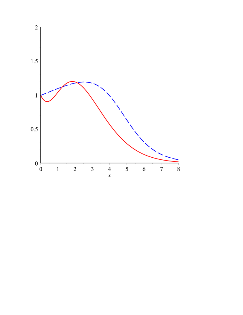
Figure 1: The function $a(x)e^{-x}=\frac{e^{\alpha/2}}{2}\left(1+\tanh\left(\frac{1}{4}(2\alpha x/(\alpha-R)-\alpha)\right)\right)e^{-x}$ defining the coefficients of the Dirichlet polynomial $\sum_{l\leqslant T}a\left(\frac{(\alpha-R)\log l}{\log T}\right)\exp\left(-\frac{(\alpha-R)\log l}{\log T}\right)l^{-(1/2+it)}$ (dash), and the approximation $\frac{e^{-x}}{s_{6}(1)}s_{6}(x+1)$ (solid)

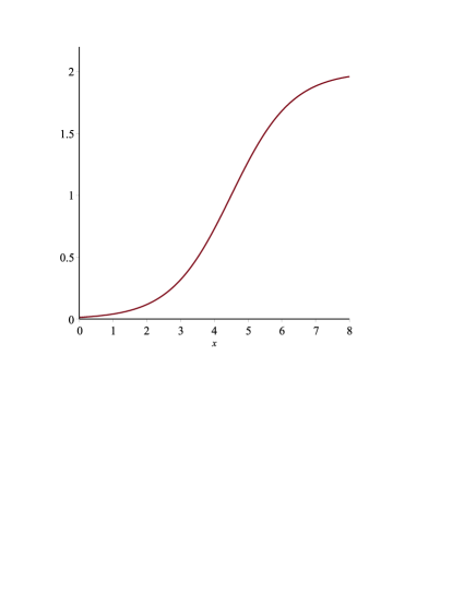
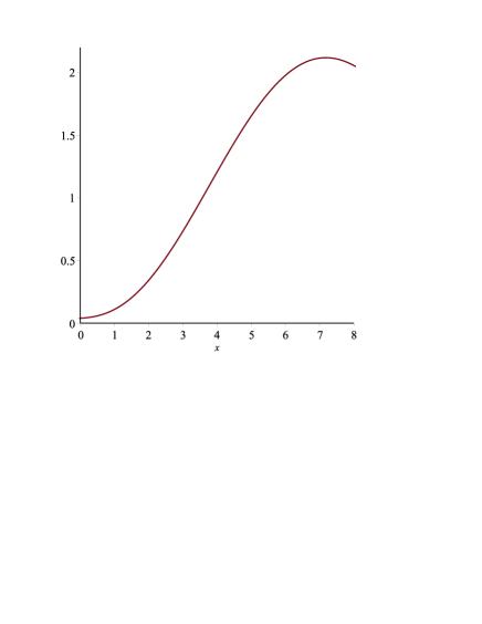
Figure 2: The function $1+\tanh\left(\frac{1}{4}(2\alpha x/(\alpha-R)-\alpha)\right)$ and the (shifted) Laguerre polynomial approximation $s_{6}(x+1)$

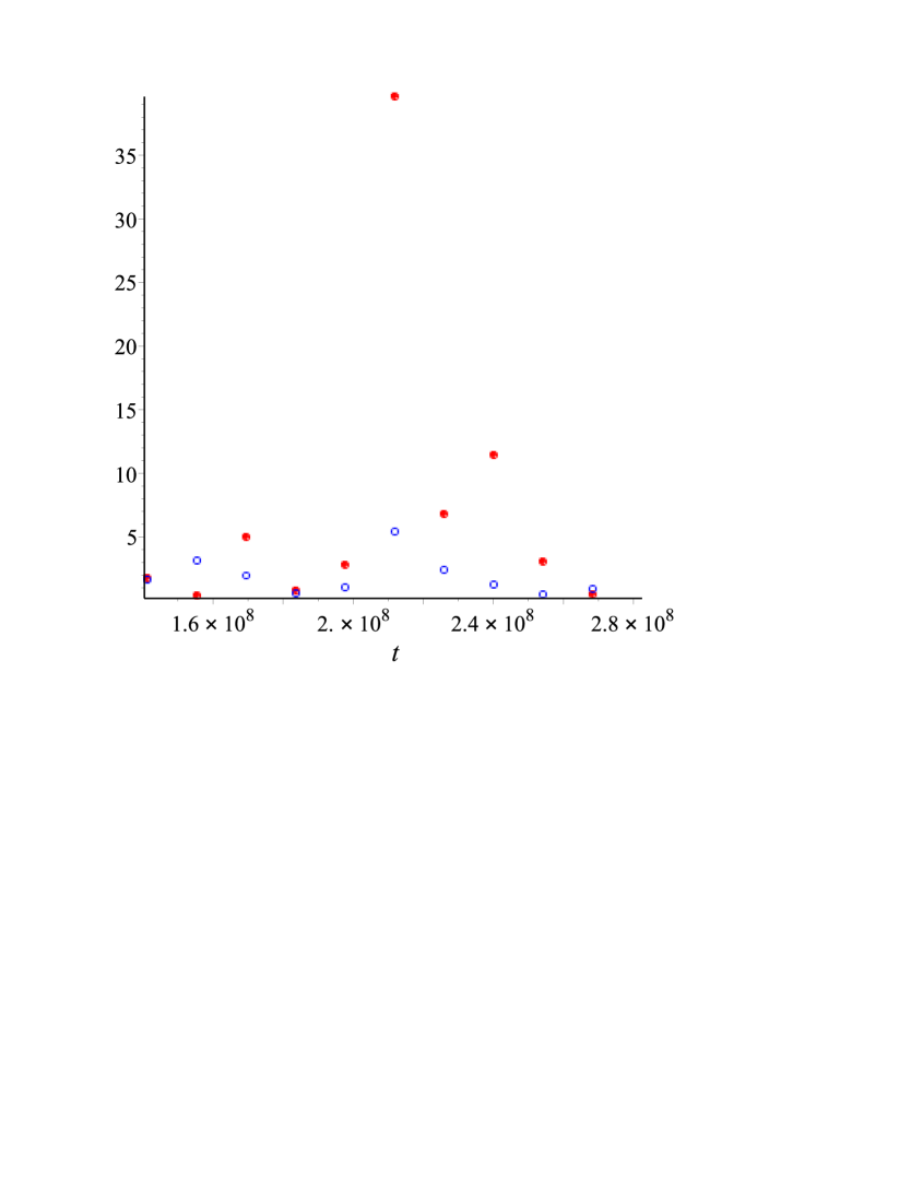
Figure 3: The absolute values of the function $\lambda\left(\frac{1}{2}+\frac{\alpha-R}{\log T}+it\right)$ (circles) for $t\in[T/2,T]$ and the majorant $A\left(\frac{1}{2}+\frac{\alpha-R}{\log T}+it\right)$ (solid circles) without lower order terms

2 Outline of the method

2.1 The Levinson–Conrey Method (A Version of the Principal Inequality)

Given real numbers $\{g_{k}\}$ let $G(s)$ be the function defined by

$$G(s)=\frac{1}{2H(s)}\left(\xi(s)+\sum_{\textup{$k$ odd}}g_{k}\xi^{(k)}(s)\right)$$

for $s\in{\mathbb{C}}$ with $s\neq 1$.

The novelty of our specific choice for $G(s)$ given in Subsection 2.2 is that it obeys the translation functional equation. It involves higher derivatives of $\zeta$ in an essential way that pushes almost all of its zeros to the region

$$\sigma\leqslant 1/2-c/\log T$$

for any fixed $c>0$. A related phenomenon is described in [Ki11, Section 3.2]. This is why our mollification is so effective.

Next, for $s=\sigma+it$ with $t\asymp T$ and $-1\leqslant\sigma\leqslant 2$ we have

$$G(s)=\sum_{l\leqslant T}Q\left(\frac{\log l}{\log T}+\delta(s)\right)l^{-s}+O\left(T^{-\frac{1}{4}}\right),$$

$\delta(s)=\frac{\log(2\pi T/s)}{2\log T}\ll\frac{1}{\log T}$, $Q(x)$ is a polynomial such that

$$Q(x)=\frac{1}{2}+\frac{1}{2}\sum\limits_{\begin{subarray}{c}k\text{{ odd}}\\ k\leqslant K\end{subarray}}g_{k}(\log T)^{k}\left(\frac{1}{2}-x\right)^{k},$$

with $g_{k}$ real (or $Q(x)+Q(1-x)=1$).

Consider

$$F(s)=G(s)M(s){\mathcal{L}}(A(s))$$

with

$$M(s)=\sum_{m\leqslant T^{\theta}}\mu(m)P\left(\frac{\log m}{\log T}\right)m^{-\left(s+\frac{R}{\log T}\right)},$$

$\theta>0$ is fixed, $P(x)$ is a real polynomial with $P(0)=1$ and $P(\theta)=0$,

$$A(s)=\sum_{m\leqslant X}\widetilde{\Lambda}(m)m^{-s}$$

is a Dirichlet polynomial with $\widetilde{\Lambda}(1)=0$. Here $X=T^{c}$ with $c$ depending on $\alpha$, $\alpha$ is a sufficiently slowly growing function of $T$, and ${\mathcal{L}}(w)$ is a polynomial such that ${\mathcal{L}}(0)=\frac{1}{Q(0)}$. Moreover, suppose that the coefficients $c(m)$ of the Dirichlet polynomial $M(s){\mathcal{L}}(A(s))$ satisfy the bound $c(m)\ll m^{\varepsilon}$, where the implied constant can depend on $\alpha$.

The following theorem represents a version of the principal inequality of the Levinson–Conrey method:

Theorem 2.

Let $R$ be fixed, $R>0$, $T$ be a parameter going to infinity,

$$a=\frac{1}{2}-\frac{R}{\log T}.$$

Let $N_{00}(T,2T)$ be the number of zeros $\rho=\frac{1}{2}+i\gamma$, $T\leqslant\gamma\leqslant 2T$, of $\zeta(s)$ counted without multiplicity, which are not zeros of $G(s)$. Let $E$ be a subset of $[T,2T]$ which has the measure $\varepsilon_{E}T$, $0<\varepsilon_{E}<1$, and is a union of a finite number of intervals. Then

$$N_{00}(T,2T)\geqslant N(T,2T)\left(1-\frac{2}{R}(\log I(R)+\varepsilon_{E}\log I_{E}(R)+L_{E}(R))+O\left(\frac{1}{\log T}\right)\right),$$

where

$$I(R)=\frac{1}{T-\varepsilon_{E}T}\int\limits_{[T,2T]\setminus E}|F(a+it)|\,dt,$$

$$I_{E}(R)=\frac{1}{\varepsilon_{E}T}\int\limits_{E}\frac{|F(a+it)|}{|{\mathcal{L}}(A(a+it))|}\,dt$$

and

$$L_{E}(R)=\frac{1}{T}\int\limits_{E}\log|{\mathcal{L}}(A(a+it))|\,dt.$$

Proof of the theorem is given in Section 4.

2.2 The Functional Equation

Definition. For $\mathop{\text{{Re}}}s>1$ define

$$g_{\alpha,T}(s)\mathrel{:=}-\frac{1}{2}\sum_{l=1}^{\infty}\tanh\left(\frac{\alpha}{2}\left(\frac{\log l}{\log T}-\frac{1}{2}\right)\right)l^{-s}.$$

In Sections 5 and 6 we will prove

1. For $\Delta\sigma=\frac{\alpha}{\log T}$ we have $2e^{\alpha/2}\left(\frac{\zeta(s+\Delta\sigma)}{2}-g_{\alpha,T}(s+\Delta\sigma)\right)=2\left(\frac{\zeta(s)}{2}+g_{\alpha,T}(s)\right)$.

2. For $s=\sigma+it$, $T\leqslant t\leqslant 2T$, the function $H(s)g_{\alpha,T}(s)+\text{small perturbation}$ is purely imaginary for $\mathop{\text{{Re}}}s=\frac{1}{2}$. The small perturbation term does not affect the principal inequality of the Levinson–Conrey method as $\alpha$ goes to infinity.

The translation functional equation of item 1 implies

$$G(s)=\sum_{l\leqslant T}\left(\frac{1}{2}+q\left(\frac{\log l}{\log T}+\delta(s)\right)\right)l^{-s}+O(T^{-\frac{1}{4}})=e^{\alpha/2}\sum_{l\leqslant T}\left(\frac{1}{2}-\widetilde{q}\left(\frac{\log l}{\log T}+\delta_{1}(s)\right)\right)l^{-(s+\Delta\sigma)}+{\mathcal{R}}.$$

The term $\delta_{1}(s)=\delta(s+\Delta\sigma)$ and ${\mathcal{R}}$ comes from a careful approximation of $-\frac{1}{2}\tanh\left(\frac{\alpha}{2}\left(\frac{\log l}{\log T}-\frac{1}{2}\right)\right)$ by polynomials $q\left(\frac{\log l}{\log T}\right)$ and $\widetilde{q}\left(\frac{\log l}{\log T}\right)$ of large degrees $K\asymp\alpha$ and $\mathcal{K}\asymp\alpha$, respectively — see Equations (6) and (7) in Section 6 below.

In the right-hand side we denote

$$G^{*}(s+\Delta\sigma)\mathrel{:=}e^{\alpha/2}\sum_{l\leqslant T}\left(\frac{1}{2}-\widetilde{q}\left(\frac{\log l}{\log T}\right)\right)l^{-(s+\Delta\sigma)}.$$

Theorem 3.

In Theorem 2 the function

$$F(s)=G(s)M(s){\mathcal{L}}(A(s))$$

can be replaced by

$$F^{*}(s)=G^{*}(s+\Delta\sigma)M(s){\mathcal{L}}(A(s))$$

with an acceptable error for $\kappa$, i.e. the error goes to $0$ as $\alpha$ and the degrees $K\asymp\alpha$, $\mathcal{K}\asymp\alpha$ of the polynomials $q$ and $\widetilde{q}$ go to infinity (the conditions on $M(s)$ and ${\mathcal{L}}(w)$ remain unchanged).

Remark. For $\Delta\sigma=\frac{\alpha}{\log T}$ we can write

$$\frac{G^{*}(s+\Delta\sigma)+O(T^{-\frac{1}{4}})}{\zeta(s+\Delta\sigma)}=c_{0}(\alpha)+\lambda(s+\Delta\sigma),$$

where $c_{0}(\alpha)=(1+o(1))\frac{e^{\alpha/2}}{2}\left(1-\tanh\left(\frac{\alpha}{4}\right)\right)$ and

$$\lambda(s+\Delta\sigma)=\frac{c_{1}(\alpha)}{\log T}\frac{\zeta^{\prime}}{\zeta}(s+\Delta\sigma)+\dots+\frac{c_{\mathcal{K}}(\alpha)}{(\log T)^{\mathcal{K}}}\frac{\zeta^{(\mathcal{K})}}{\zeta}(s+\Delta\sigma)$$

with the coefficients $c_{1}(\alpha)$, $c_{2}(\alpha)$, $\dots$, $c_{\mathcal{K}}(\alpha)$ implicitly defined by the polynomial $\widetilde{q}\left(\frac{\log l}{\log T}\right)$.

2.3 Theorems of Selberg and Lester (A Generalization)

Theorem 4.

Let $T\leqslant t\leqslant 2T$, $x=T^{1/\alpha^{1/2+4C}}$, $x_{0}=T^{1/\alpha^{4C}}$, $x_{1}=T^{1/\alpha^{1/2+8C}}$,

$$\Delta\sigma=\frac{\alpha}{\log T},$$

with $\alpha$ going to infinity with $T$ sufficiently slowly, $R=\varepsilon\log\alpha$, $\varepsilon>0$ sufficiently small and $C\geqslant\frac{1}{8}$ sufficiently large be fixed, and $\sigma+\Delta\sigma=\frac{1}{2}+\frac{\alpha-R}{\log T}$. Let $\frac{\gamma(k,(\alpha-R)/2)}{\gamma(k,\alpha-R)}$ be the ratio of the lower incomplete gamma functions. Then there exists a set ${\mathcal{M}}_{\alpha}\subset[T,2T]$ with $\mathop{\text{{meas}}}{\mathcal{M}}_{\alpha}\geqslant(1-\alpha^{1-C(1-\varepsilon)})T$ such that for each $t\in{\mathcal{M}}_{\alpha}$ we have the following Selberg estimate for $\lambda(\sigma+\Delta\sigma+it)$, see (11):

$$\lambda(\sigma+\Delta\sigma+it)\ll\left|\sum_{k=1}^{\mathcal{K}}\frac{|c_{k}(\alpha)|\gamma(k,(\alpha-R)/2)}{\gamma(k,\alpha-R)(\log T)^{k}}\sum_{\begin{subarray}{c}R_{1}\geqslant 0,\ldots,R_{k}\geqslant 0\\ R_{1}+\dots+kR_{k}=k\end{subarray}}\frac{k!}{R_{1}!\dots R_{k}!}\prod_{j=1}^{k}\left(\frac{A_{j}(\sigma+\Delta\sigma+it)}{j!}\right)^{R_{j}}\right|,$$

where

$$\begin{split}A_{j}(\sigma+\Delta\sigma+it)=&\frac{j!(\log T)^{j}}{(\alpha-R-C\log\alpha)^{j}}\sum_{n\leqslant x_{0}^{3}}\frac{\Lambda_{x_{0}}(n)}{\log n}\left(\frac{2}{n^{\sigma+\Delta\sigma+(\alpha^{1/2+4C}-\alpha+R)/\log T+it}}\right.\\ &\left.-\frac{1}{n^{\sigma+\Delta\sigma+(\alpha^{1/2+8C}-\alpha+R)/\log T+it}}\right)\\ &+\frac{\alpha^{1/2+4C}}{\log T}\frac{j!(\log T)^{j}}{(\alpha-R-C\log\alpha)^{j}}\left(\sum_{n\leqslant x^{3}}\frac{\Lambda_{x}(n)}{n^{\sigma+\Delta\sigma+(\alpha^{1/2+4C}-\alpha+R)/\log T+it}}\right.\\ &\left.+\sum_{n\leqslant x_{0}^{3}}\frac{\Lambda_{x_{0}}(n)}{n^{\sigma+\Delta\sigma+(\alpha^{1/2+4C}-\alpha+R)/\log T+it}}+\sum_{n\leqslant x_{0}^{3}}\frac{\Lambda_{x_{0}}(n)}{n^{\sigma+\Delta\sigma+(\alpha^{1/2+8C}-\alpha+R)/\log T+it}}\right)\\ &+\frac{\alpha^{1/2+8C}}{\log T}\frac{j!(\log T)^{j}}{(\alpha-R-C\log\alpha)^{j}}\sum_{n\leqslant x_{1}^{3}}\frac{\Lambda_{x_{1}}(n)}{n^{\sigma+\Delta\sigma+(\alpha^{1/2+8C}-\alpha+R)/\log T+it}}\\ &+e^{-\sqrt{\alpha}}\left.\left(\frac{d}{ds_{1}}\right)^{j}\int\limits_{s_{1}}^{s_{1}+\frac{\alpha^{1/2+8C}-\alpha+R}{\log T}}\log s\,ds\right|_{s_{1}=\sigma+\Delta\sigma+it}.\end{split}$$

We prove Theorem 4 in Section 8.

Now for all $t\in[T,2T]$ we denote

$$A(\sigma+\Delta\sigma+it)\mathrel{:=}\sum_{k=1}^{\mathcal{K}}\frac{|c_{k}(\alpha)|\gamma(k,(\alpha-R)/2)}{\gamma(k,\alpha-R)(\log T)^{k}}\sum_{\begin{subarray}{c}R_{1}\geqslant 0,\ldots,R_{k}\geqslant 0\\ R_{1}+\dots+kR_{k}=k\end{subarray}}\frac{k!}{R_{1}!\dots R_{k}!}\prod_{j=1}^{k}\left(\frac{A_{j}(\sigma+\Delta\sigma+it)}{j!}\right)^{R_{j}}.$$

The behavior of this Dirichlet polynomial $A(\sigma+\Delta\sigma+it)$ is controlled by rough analogs (see (17), (18)) of the following theorems of Lester.

Let $\psi(T)=(2\sigma-1)\log T$, and for $\psi(T)\geqslant 1$ define $V=V(\sigma)=\frac{1}{2}\sum_{n=2}^{\infty}\frac{\Lambda^{2}(n)}{n^{2\sigma}}$, $\Omega=e^{-10}\min\big{(}V^{3/2},(\psi(T)/\log\psi(T))^{1/2}\big{)}$. Suppose that $\psi(T)\to\infty$ with $T$, and $\psi(T)=o(\log T)$.

Theorem (Lester’s Theorem for a Rectangle). Let $R$ be a rectangle in $\mathbb{C}$ whose sides are parallel to the coordinate axes. Then we have

$$\mathop{\text{{meas}}}\bigg{\{}t\in(0,T):\frac{\zeta^{\prime}}{\zeta}(\sigma+it)V^{-1/2}\in R\bigg{\}}=\frac{T}{2\pi}\iint_{R}\!e^{-(x^{2}+y^{2})/2}\,dx\,dy+O\left(T\frac{(\mathop{\text{{meas}}}(R)+1)}{\Omega}\right).$$

Theorem (Lester’s Theorem for a Disk). Let $r$ be a real number such that $r\Omega\geqslant 1$. Then we have

$$\mathop{\text{{meas}}}\bigg{\{}t\in(0,T):\bigg{|}\frac{\zeta^{\prime}}{\zeta}(\sigma+it)\bigg{|}\leqslant\sqrt{V}r\bigg{\}}=\,T(1-e^{-r^{2}/2})+O\left(T\left(\frac{r^{2}+r}{\Omega}\right)\right).$$

In Section 9 we construct the Dirichlet polynomial ${\mathcal{L}}(A(s))$ that approximates the function $\frac{\widetilde{\mathcal{M}}}{c_{0}+A(s)}$ for almost all values of $t$. Hence in the term

$$\begin{split}&\frac{2}{R}\log I(R)=\frac{2}{R}\log\left(\frac{1}{T-\varepsilon_{E}T}\int\limits_{[T,2T]\setminus E}|G^{*}(\sigma+\Delta\sigma+it)M(\sigma+it){\mathcal{L}}(A(\sigma+\Delta\sigma+it))|\,dt\right)\\ &=\frac{2}{R}\\ &\times\log\left(\frac{1}{T-\varepsilon_{E}T}\int\limits_{[T,2T]\setminus E}|\zeta(\sigma+\Delta\sigma+it)\bigg{(}c_{0}+\lambda(\sigma+\Delta\sigma+it)\bigg{)}M(\sigma+it){\mathcal{L}}(A(\sigma+\Delta\sigma+it))|\,dt\right)\end{split}$$

of the principal inequality of the Levinson–Conrey method, the product

$$\bigg{(}c_{0}+\lambda(\sigma+\Delta\sigma+it)\bigg{)}{\mathcal{L}}(A(\sigma+\Delta\sigma+it))$$

is ${}\ll\widetilde{\mathcal{M}}$ and we will choose $\frac{\log\widetilde{\mathcal{M}}}{R}$ to be small.

Now it remains to estimate the integral

$$\frac{1}{T-\varepsilon_{E}T}\int\limits_{[T,2T]\setminus E}|\zeta(\sigma+\Delta\sigma+it)M(\sigma+it)|\,dt$$

for the translated zeta-function $\zeta(\sigma+\Delta\sigma+it)$ and its optimal mollifier $M(\sigma+it)$ (of length $T^{1/2}$, say). This is done using the mean-square asymptotics. Since $\sigma+\Delta\sigma=\frac{1}{2}+\frac{\alpha-R}{\log T}$ and we make $\alpha\to\infty$ (slowly) as $T\to\infty$, this integral is close to $1$.

The remaining terms in the principal inequality of the Levinson–Conrey method, namely, $\varepsilon_{E}\log I_{E}(R)$ and $L_{E}(R)$, are proven to give a negligible contribution.

We now proceed to details of the argument.

3 Translation lemmas

Lemma 1.

Let $f(s)$ be an analytic function, $s\in{\mathbb{C}}$, $\Delta\sigma\in{\mathbb{R}}$, $\mathcal{K}\geqslant 1$ be an odd integer. Then

$$\begin{split}&f(s+\Delta\sigma)=f(s)+\sum_{\begin{subarray}{c}k\text{{ odd}}\\ k\leqslant\mathcal{K}\end{subarray}}\left(g_{k}(\Delta\sigma)f^{(k)}(s)+g_{k}(\Delta\sigma)f^{(k)}(s+\Delta\sigma)\right)\\ &+\frac{4(-1)^{(\mathcal{K}+1)/2}(\Delta\sigma)^{\mathcal{K}+1}}{\pi^{\mathcal{K}+2}}\int\limits_{s}^{s+\Delta\sigma}f^{(\mathcal{K}+2)}(w)\left(\sum_{n=1}^{\infty}\frac{1}{(2n-1)^{\mathcal{K}+2}}\sin\left(\frac{(2n-1)\pi(s+\Delta\sigma-w)}{\Delta\sigma}\right)\right)\,dw,\end{split}$$ (1)

where

$$g_{k}(\Delta\sigma)=\frac{4(-1)^{(k-1)/2}(\Delta\sigma)^{k}}{\pi^{k+1}}\sum_{n=1}^{\infty}\frac{1}{(2n-1)^{k+1}}.$$

Proof. We induct on $\mathcal{K}$. First establish induction base $\mathcal{K}=1$. We have

$$f(s+\Delta\sigma)=f(s)+\int\limits_{s}^{s+\Delta\sigma}f^{\prime}(w)\,dw.$$

Let $\mathop{\text{{sgn}}_{2\Delta\sigma}}(x)$ be the $2\Delta\sigma$-periodic real-valued function defined by

$$\mathop{\text{{sgn}}_{2\Delta\sigma}}(x)=\begin{cases}1&\text{if $x\in(0,\Delta\sigma)$},\\ 0&\text{if $x=-\Delta\sigma,0,\Delta\sigma$},\\ -1&\text{if $x\in(-\Delta\sigma,0)$}.\end{cases}$$

Using the Fourier expansion

$$\mathop{\text{{sgn}}_{2\Delta\sigma}}(x)=\frac{4}{\pi}\sum_{n=1}^{\infty}\frac{1}{2n-1}\sin\left(\frac{(2n-1)\pi x}{\Delta\sigma}\right)$$ (2)

we obtain

$$\begin{split}f(s+\Delta\sigma)&=f(s)+\frac{4}{\pi}\int\limits_{s}^{s+\Delta\sigma}f^{\prime}(w)\left(\sum_{n=1}^{\infty}\frac{1}{2n-1}\sin\left(\frac{(2n-1)\pi(s+\Delta\sigma-w)}{\Delta\sigma}\right)\right)\,dw.\end{split}$$

If the range of integration is split over $I_{1}=[s,s+\varepsilon]$, $I_{2}=[s+\varepsilon,s+\Delta\sigma-\varepsilon]$, $I_{3}=[s+\Delta\sigma-\varepsilon,s+\Delta\sigma]$ then the integrals over $I_{1}$ and $I_{3}$ go to $0$ as $\varepsilon\to 0$. The series (2) converges uniformly in $x\in[\varepsilon,\Delta\sigma-\varepsilon]$ so by integrating by parts over $I_{2}$

$$\begin{split}&\frac{4}{\pi}\int\limits_{s+\varepsilon}^{s+\Delta\sigma-\varepsilon}f^{\prime}(w)\,d\left(\sum_{n=1}^{\infty}\frac{\Delta\sigma}{(2n-1)^{2}\pi}\cos\left(\frac{(2n-1)\pi(s+\Delta\sigma-w)}{\Delta\sigma}\right)\right)\\ \mathrel{=}&\frac{4\Delta\sigma}{\pi^{2}}\sum_{n=1}^{\infty}\frac{1}{(2n-1)^{2}}\Bigl{(}f^{\prime}(s+\Delta\sigma-\varepsilon)+f^{\prime}(s+\varepsilon)\Bigr{)}\\ -&\frac{4\Delta\sigma}{\pi^{2}}\int\limits_{s+\varepsilon}^{s+\Delta\sigma-\varepsilon}f^{\prime\prime}(w)\left(\sum_{n=1}^{\infty}\frac{1}{(2n-1)^{2}}\cos\left(\frac{(2n-1)\pi(s+\Delta\sigma-w)}{\Delta\sigma}\right)\right)\,dw+\delta_{1}(\varepsilon)\\ \mathrel{=}&g_{1}(\Delta\sigma)\Bigl{(}f^{\prime}(s)+f^{\prime}(s+\Delta\sigma)\Bigr{)}\\ -&\frac{4\Delta\sigma}{\pi^{2}}\int\limits_{s}^{s+\Delta\sigma}f^{\prime\prime}(w)\,d\left(\sum_{n=1}^{\infty}-\frac{\Delta\sigma}{(2n-1)^{3}\pi}\sin\left(\frac{(2n-1)\pi(s+\Delta\sigma-w)}{\Delta\sigma}\right)\right)+\delta_{2}(\varepsilon)\\ \mathrel{=}&g_{1}(\Delta\sigma)\Bigl{(}f^{\prime}(s)+f^{\prime}(s+\Delta\sigma)\Bigr{)}\\ -&\frac{4\Delta\sigma}{\pi^{2}}\left(-\int\limits_{s}^{s+\Delta\sigma}-\frac{\Delta\sigma}{\pi}f^{\prime\prime\prime}(w)\left(\sum_{n=1}^{\infty}\frac{1}{(2n-1)^{3}}\sin\left(\frac{(2n-1)\pi(s+\Delta\sigma-w)}{\Delta\sigma}\right)\right)dw\right)+\delta_{3}(\varepsilon),\end{split}$$

and $\delta_{1}(\varepsilon),\delta_{2}(\varepsilon),\delta_{3}(\varepsilon)\to 0$ as $\varepsilon\to 0$. This proves the induction base. The induction step is proven by integrating by parts in (1) as above, with the uniform convergence of the series in the integrand when $\mathcal{K}\geqslant 1$.

Remark. We have

$$g_{1}(\Delta\sigma)=\frac{4\Delta\sigma}{\pi^{2}}\sum_{n=1}^{\infty}\frac{1}{(2n-1)^{2}}=\frac{4\Delta\sigma}{\pi^{2}}\zeta(2)\left(1-\frac{1}{2^{2}}\right)=\frac{\Delta\sigma}{2},$$

and in general for $k$ odd

$$g_{k}(\Delta\sigma)=\frac{4(-1)^{(k-1)/2}(\Delta\sigma)^{k}}{\pi^{k+1}}\zeta(k+1)\left(1-\frac{1}{2^{k+1}}\right)=-\left(\frac{\Delta\sigma}{2}\right)^{k}\frac{2^{k+1}-4^{k+1}}{(k+1)!}B_{k+1},$$ (3)

where $B_{k+1}$ is the Bernoulli number.

The series

$$\sum_{\begin{subarray}{c}k\geqslant 1\\ k\text{{ odd}}\end{subarray}}\left(g_{k}(\Delta\sigma)f^{(k)}(s)+g_{k}(\Delta\sigma)f^{(k)}(s+\Delta\sigma)\right)$$

obtained by successive integrations by parts in (1) may be divergent. However, we have the following Lemma 2. Note that if in the series

$$\sum_{\begin{subarray}{c}k\geqslant 1\\ k\text{{ odd}}\end{subarray}}\Bigl{(}-g_{k}(\Delta\sigma)\Bigr{)}(\log T)^{k}\left(\frac{1}{2}-x\right)^{k}$$

considered in Lemma 2, we substitute $x=\frac{\log l}{\log T}$, multiply over by $l^{-(s+\Delta\sigma)}$ and sum over $l$ from $1$ to $T$, then we get an approximation for

$$H(s+\Delta\sigma)^{-1}\sum_{\begin{subarray}{c}k\geqslant 1\\ k\text{{ odd}}\end{subarray}}\Bigl{(}-g_{k}(\Delta\sigma)\Bigr{)}{\xi}^{(k)}(s+\Delta\sigma)$$

(see [Iw14, Chapter 18, (18.9)]).

Lemma 2.

Suppose that $0<\varepsilon<2\pi$, $|\alpha|\leqslant 2\pi-\varepsilon$ and

$$|\Delta\sigma|=\frac{|\alpha|}{\log T}\leqslant\frac{2\pi-\varepsilon}{\log T}.$$

Then the series

$$\sum_{\begin{subarray}{c}k\geqslant 1\\ k\text{{ odd}}\end{subarray}}\Bigl{(}-g_{k}(\Delta\sigma)\Bigr{)}(\log T)^{k}\left(\frac{1}{2}-x\right)^{k}$$

converges on $x\in[0,1]$ and

$$\sum_{\begin{subarray}{c}k\geqslant 1\\ k\text{{ odd}}\end{subarray}}\Bigl{(}-g_{k}(\Delta\sigma)\Bigr{)}(\log T)^{k}\left(\frac{1}{2}-x\right)^{k}=-\tanh\left(\frac{\alpha}{2}\left(\frac{1}{2}-x\right)\right).$$

Proof. By the definition of the Bernoulli numbers,

$$\frac{z}{e^{z}-1}=\sum_{m=0}^{\infty}\frac{B_{m}}{m!}z^{m},$$

with $B_{0}=1$, $B_{1}=-\frac{1}{2}$ and $B_{3}=B_{5}=B_{7}=\dots=0$, the radius of convergence of the series being $2\pi$.

Since for $|z|\leqslant\pi/2-\varepsilon$

$$\tanh(z)=\sum_{n\geqslant 1}\frac{2^{2n}\left(2^{2n}-1\right)B_{2n}}{(2n)!}z^{2n-1},$$

then

$$-\tanh\left(\frac{\alpha}{2}\left(\frac{1}{2}-x\right)\right)=\sum_{\begin{subarray}{c}k\geqslant 1\\ k\text{{ odd}}\end{subarray}}\frac{(2^{k+1}-4^{k+1})B_{k+1}}{(k+1)!}\frac{\alpha^{k}}{2^{k}}\left(\frac{1}{2}-x\right)^{k}$$

and the lemma follows from (3).

The following lemma is an easy consequence of Stirling’s formula.

Lemma 3.

Suppose that $\alpha$ is real and

$$\Delta\sigma=\frac{\alpha}{\log T}.$$

Then in the rectangle

$$s=\sigma+it,\quad\frac{1}{3}\leqslant\sigma\leqslant A,\quad T\leqslant t\leqslant 2T$$

with $A\geqslant 3$ and $T\geqslant 2A$ we have

$$H(s+\Delta\sigma)=\left(e^{\alpha/2}+O_{\alpha}\left(\frac{1}{\log T}\right)\right)H(s).$$

Thus Lemmas 1 (with Remark), 2, 3 allow one to replace

$$e^{\alpha/2}\sum_{l=1}^{T}\left(1+\tanh\left(\frac{\alpha}{2}\left(\frac{\log l}{\log T}-\frac{1}{2}\right)\right)\right)l^{-(s+\Delta\sigma)}$$

by

$$\sum_{l=1}^{T}\left(1-\tanh\left(\frac{\alpha}{2}\left(\frac{\log l}{\log T}-\frac{1}{2}\right)\right)\right)l^{-s}$$

plus some error, i.e. to link the value of the function suitable for the Levinson–Conrey method at $s$ to the value of the similarly looking function at $s+\Delta\sigma$, yet subject to $|\alpha|<2\pi$. In Section 5 we shall get rid of this constraint.

4 A version of the principal inequality of the Levinson–Conrey method

For a detailed exposition of the Levinson–Conrey method, see [Con89], [Iw14].

Suppose that in the rectangle

$$s=\sigma+it,\quad\frac{1}{3}\leqslant\sigma\leqslant A,\quad T\leqslant t\leqslant 2T,$$

with $A\geqslant 3$ and $T\geqslant 2A$, function $G(s)$ is of the form

$$G(s)=\sum_{l\leqslant T}Q\left(\frac{\log l}{\log T}+\delta(s)\right)l^{-s}+O\left(T^{-\frac{1}{4}}\right),$$

where

$$\delta(s)=\frac{\log(2\pi T/s)}{2\log T}\ll\frac{1}{\log T},$$

and $Q(x)$ is a polynomial such that

$$Q(x)=\frac{1}{2}+\frac{1}{2}\sum_{\begin{subarray}{c}k\text{{ odd}}\\ k\leqslant\mathcal{K}\end{subarray}}g_{k}(\log T)^{k}\left(\frac{1}{2}-x\right)^{k},$$

where $g_{k}$ are real (the equation is equivalent to $Q(x)+Q(1-x)=1$).

Next, consider

$$F(s)=G(s)M(s){\mathcal{L}}(A(s))$$

with the mollifiers

$$M(s)=\sum_{m\leqslant T^{\theta}}\mu(m)P\left(\frac{\log m}{\log T}\right)m^{-\left(s+\frac{R}{\log T}\right)},$$

where $P(x)$ is a real polynomial with

$$P(0)=1\qquad\text{and}\qquad P(\theta)=0,$$

$A(s)$ is a Dirichlet polynomial

$$A(s)=\sum_{m\leqslant X}\widetilde{\Lambda}(m)m^{-s}$$

with $\widetilde{\Lambda}(1)=0$ (here $X=T^{c}$ with $c$ depending on $\alpha$), and ${\mathcal{L}}(w)$ is a polynomial such that ${\mathcal{L}}(0)=\frac{1}{Q(0)}$. Moreover, suppose that the coefficients $c(m)$ of the Dirichlet polynomial $M(s){\mathcal{L}}(A(s))$ satisfy the bound $c(m)\ll m^{\varepsilon}$, where the implied constant can depend on $\alpha$.

We now prove Theorem 2, Subsection 2.1 which represents a version of the principal inequality of the Levinson–Conrey method.

Proof of Theorem 2. The inequality

$$N_{00}(T,2T)\geqslant N(T,2T)\left(1-\frac{2}{R}l(R)+O\left(\frac{1}{\log T}\right)\right)$$

where $l(R)=\frac{1}{T}\int_{T}^{2T}\log|F(a+it)|\,dt$ is provided in [Iw14, Chapter 22, (22.4) and (22.5)].

Our function $F(s)$ has additional mollifier ${\mathcal{L}}(A(s))$. The difference between our mollifier and the one in the book is that our constants can depend on $\alpha$. But in our argument we can suppose that $\alpha$ is fixed. The larger $\alpha$ we take, the closer we approach $\varkappa=1$ in the end. Eventually we can take $\alpha$ to be a sufficiently slowly growing function of $T$.

Next we write

$$\begin{split}&\frac{1}{T}\int_{T}^{2T}\log|F(a+it)|\,dt\leqslant\frac{1}{T-\varepsilon_{E}T}\int\limits_{[T,2T]\setminus E}\log|F(a+it)|\,dt\\ &+\frac{\varepsilon_{E}}{\varepsilon_{E}T}\int\limits_{E}\log\frac{|F(a+it)|}{|{\mathcal{L}}(A(a+it))|}\,dt+\frac{1}{T}\int\limits_{E}\log|{\mathcal{L}}(A(a+it))|\,dt.\end{split}$$

The inequalities

$$\frac{1}{T-\varepsilon_{E}T}\int\limits_{[T,2T]\setminus E}\log|F(a+it)|\,dt\leqslant\log\left(\frac{1}{T-\varepsilon_{E}T}\int\limits_{[T,2T]\setminus E}|F(a+it)|\,dt\right)$$

and

$$\frac{1}{\varepsilon_{E}T}\int\limits_{E}\log\frac{|F(a+it)|}{|{\mathcal{L}}(A(a+it))|}\,dt\leqslant\log\left(\frac{1}{\varepsilon_{E}T}\int\limits_{E}\frac{|F(a+it)|}{|{\mathcal{L}}(A(a+it))|}\,dt\right)$$

follow by considering the integral sums and using arithmetic–geometric mean inequality.

5 Function $g_{\alpha,T}(s)$

In the subsequent arguments we shall get rid of the limitation $|\alpha|<2\pi$ in Lemma 2 by showing that for $\alpha$ arbitrarily large the analytic function given for $\mathop{\text{{Re}}}s>1$ by

$$g_{\alpha,T}(s)=-\frac{1}{2}\sum_{l=1}^{\infty}\tanh\left(\frac{\alpha}{2}\left(\frac{\log l}{\log T}-\frac{1}{2}\right)\right)l^{-s}$$

obeys two types of symmetries:

1. For $\Delta\sigma=\frac{\alpha}{\log T}$

   $$2e^{\alpha/2}\left(\frac{\zeta(s+\Delta\sigma)}{2}-g_{\alpha,T}(s+\Delta\sigma)\right)=2\left(\frac{\zeta(s)}{2}+g_{\alpha,T}(s)\right).$$ (4)

2. For $s=\sigma+it$, $T\leqslant t\leqslant 2T$, the function

   $$H(s)g_{\alpha,T}(s)$$ (5)

   is approximated by a sum of the odd derivatives of the $\xi$ function with real coefficients which are purely imaginary for $\mathop{\text{{Re}}}s=\frac{1}{2}$.

To prove (4) we note that

$$e^{-u}\left(1+\tanh\left(\frac{u}{2}\right)\right)=1-\tanh\left(\frac{u}{2}\right).$$

Now take

$$u=\alpha\left(\frac{\log l}{\log T}-\frac{1}{2}\right)$$

multiply the first formula by $l^{-s}$ with $\mathop{\text{{Re}}}s>1$ and sum over $l\geqslant 1$.

We shall prove (5) in Lemma 6.

In the following section, we shall describe properties of $g_{\alpha,T}(s)$ in detail.

6 Properties of $g_{\alpha,T}(s)$

Lemma 4 (Analytic continuation of $g_{\alpha,T}(s)$).

For $s=\sigma+it$ with $\sigma>0$ and $0<t_{0}\leqslant|t|\leqslant 2T$, where $t_{0}$ is fixed and $T\geqslant 1$, and for integer $N\geqslant T$ we have

$$\begin{split}g_{\alpha,T}(s)=-\frac{1}{2}&\left(\sum_{n=1}^{N}\tanh\left(\frac{\alpha}{2}\left(\frac{\log n}{\log T}-\frac{1}{2}\right)\right)n^{-s}\right.\\ &\left.{}-\frac{2T^{1-s}\log T}{\alpha(e^{\alpha/2}+1)(1-(1-s)(\log T)/\alpha)}F(1,1;2-(1-s)(\log T)/\alpha;(e^{\alpha/2}+1)^{-1})\right.\\ &\left.{}+\frac{T^{1-s}}{s-1}-\int\limits_{T}^{N+1/2}\tanh\left(\frac{\alpha}{2}\left(\frac{\log u}{\log T}-\frac{1}{2}\right)\right)u^{-s}du\right.\\ &\left.{}+\frac{\alpha}{2\log T}\int\limits_{N+1/2}^{+\infty}\psi(u)\cosh^{-2}\left(\frac{\alpha}{2}\left(\frac{\log u}{\log T}-\frac{1}{2}\right)\right)u^{-s-1}du\right.\\ &\left.{}-s\int\limits_{N+1/2}^{+\infty}\psi(u)\tanh\left(\frac{\alpha}{2}\left(\frac{\log u}{\log T}-\frac{1}{2}\right)\right)u^{-s-1}du\right),\end{split}$$

where $F(a,b;c;z)$ is the hypergeometric function, and $\psi(x)=x-[x]-\frac{1}{2}$.

Proof. By the exact summation formula we have

$$\begin{split}&\sum_{N+1/2<n\leqslant M+1/2}\tanh\left(\frac{\alpha}{2}\left(\frac{\log n}{\log T}-\frac{1}{2}\right)\right)n^{-s}=\int\limits_{N+1/2}^{M+1/2}\tanh\left(\frac{\alpha}{2}\left(\frac{\log u}{\log T}-\frac{1}{2}\right)\right)u^{-s}du\\ {}+&\frac{\alpha}{2\log T}\int\limits_{N+1/2}^{M+1/2}\psi(u)\cosh^{-2}\left(\frac{\alpha}{2}\left(\frac{\log u}{\log T}-\frac{1}{2}\right)\right)u^{-s-1}du\\ {}-&s\int\limits_{N+1/2}^{M+1/2}\psi(u)\tanh\left(\frac{\alpha}{2}\left(\frac{\log u}{\log T}-\frac{1}{2}\right)\right)u^{-s-1}du.\end{split}$$

The first integral is convergent for $\sigma>1$ as $M\to+\infty$, whereas the latter two integrals with the $\psi$ function converge absolutely for $\sigma>0$. Denote them by $\Psi_{1}$ and $\Psi_{2}$. Now for $\sigma>1$ we have the formula

$$\begin{split}g_{\alpha,T}(s)=-\frac{1}{2}&\left(\sum_{n=1}^{N}\tanh\left(\frac{\alpha}{2}\left(\frac{\log n}{\log T}-\frac{1}{2}\right)\right)n^{-s}\right.\\ &\left.{}+\int\limits_{T}^{+\infty}\tanh\left(\frac{\alpha}{2}\left(\frac{\log u}{\log T}-\frac{1}{2}\right)\right)u^{-s}du-\int\limits_{T}^{N+1/2}\tanh\left(\frac{\alpha}{2}\left(\frac{\log u}{\log T}-\frac{1}{2}\right)\right)u^{-s}du\right.\\ &\left.{}+\frac{\alpha}{2\log T}\Psi_{1}-s\Psi_{2}\right),\end{split}$$

in which we consider

$$\int\limits_{T}^{+\infty}\tanh\left(\frac{\alpha}{2}\left(\frac{\log u}{\log T}-\frac{1}{2}\right)\right)u^{-s}du.$$

We write the integrand as

$$\tanh\left(\frac{\alpha}{2}\left(\frac{\log u}{\log T}-\frac{1}{2}\right)\right)u^{-s}=-\frac{2u^{-s}}{e^{-\alpha/2}u^{\alpha/\log T}+1}+u^{-s}.$$

Integrating the latter term we get $\frac{T^{1-s}}{s-1}$, while the former term gives

$$\begin{split}\int\limits_{T}^{+\infty}\frac{-2T^{-\frac{s}{2}+\frac{1}{2}}}{\left(\frac{u}{\sqrt{T}}\right)^{\frac{\alpha}{\log T}}+1}\left(\frac{u}{\sqrt{T}}\right)^{-s}d\left(\frac{u}{\sqrt{T}}\right)&=-2T^{\frac{1-s}{2}}\int\limits_{\sqrt{T}}^{+\infty}\frac{x^{-s}dx}{1+x^{\alpha/\log T}}\\ &=\frac{-2T^{\frac{1-s}{2}}\log T}{\alpha}\int\limits_{e^{\alpha/2}}^{+\infty}\frac{v^{(1-s)(\log T)/\alpha-1}}{1+v}\,dv.\end{split}$$

Making the change of variables

$$\begin{split}w&=\frac{1}{v+1},\\ v&=\frac{1}{w}-1,\\ dv&=-\frac{1}{w^{2}}\,dw\end{split}$$

we get the integral

$$\frac{-2T^{\frac{1-s}{2}}\log T}{\alpha}\int\limits_{0}^{(e^{\alpha/2}+1)^{-1}}w^{1-(1-s)(\log T)/\alpha-1}(1-w)^{(1-s)(\log T)/\alpha-1}dw$$

that can be written as the incomplete beta function

$$\frac{-2T^{\frac{1-s}{2}}\log T}{\alpha}B_{(e^{\alpha/2}+1)^{-1}}(1-(1-s)(\log T)/\alpha,(1-s)(\log T)/\alpha)$$

which in turn can be expressed in terms of the hypergeometric function

$$\begin{split}&\frac{-2T^{\frac{1-s}{2}}\log T}{\alpha}(e^{\alpha/2}+1)^{(1-s)(\log T)/\alpha}\\ &\times F\left(1-(1-s)(\log T)/\alpha,1-(1-s)(\log T)/\alpha;2-(1-s)(\log T)/\alpha;(e^{\alpha/2}+1)^{-1}\right).\end{split}$$

Using the known linear transformation formula

$$F(a,b;c;z)=(1-z)^{c-a-b}F(c-a,c-b;c;z)$$

we get the term

$$-\frac{2T^{1-s}\log T}{\alpha(e^{\alpha/2}+1)(1-(1-s)(\log T)/\alpha)}F(1,1;2-(1-s)(\log T)/\alpha;(e^{\alpha/2}+1)^{-1})$$

of the analytic continuation formula, where the function

$$F(1,1;2-(1-s)(\log T)/\alpha;(e^{\alpha/2}+1)^{-1})$$

is analytic and bounded in $s$ for $|t|\geqslant t_{0}>0$ by the series representation.

Lemma 5 (Approximate equation for $g_{\alpha,T}(s)$).

For $s=\sigma+it$ with $\sigma\geqslant\sigma_{0}>0$ and $0<t_{0}\leqslant|t|\leqslant 2T$, where $\sigma_{0}$, $t_{0}$ are fixed and $T\geqslant 1$, we have

$$\begin{split}g_{\alpha,T}(s)=-\frac{1}{2}&\left(\sum_{n=1}^{T}\tanh\left(\frac{\alpha}{2}\left(\frac{\log n}{\log T}-\frac{1}{2}\right)\right)n^{-s}\right.\\ &\left.{}-\frac{2T^{1-s}\log T}{\alpha(e^{\alpha/2}+1)(1-(1-s)(\log T)/\alpha)}F(1,1;2-(1-s)(\log T)/\alpha;(e^{\alpha/2}+1)^{-1})\right.\\ &\left.{}+\frac{T^{1-s}}{s-1}+O\left(T^{-\sigma}\right)\right),\end{split}$$

where the constant in the $O$-term is absolute.

Proof. In the analytic continuation formula of Lemma 4 we use the standard uniform approximation

$$\sum_{T<n\leqslant N+1/2}\tanh\left(\frac{\alpha}{2}\left(\frac{\log n}{\log T}-\frac{1}{2}\right)\right)n^{-s}=\int\limits_{T}^{N+1/2}\tanh\left(\frac{\alpha}{2}\left(\frac{\log u}{\log T}-\frac{1}{2}\right)\right)u^{-s}du+O\left(T^{-\sigma}\right)$$

and make $N\to\infty$. ∎

We now obtain approximations to $g_{\alpha,T}(s)$ that we need in the context of Conrey’s construction [Iw14, Chapter 18]. First, we approximate it by using the Fourier expansion

$$\tanh\left(\frac{\alpha x}{2}\right)=\sum_{k=1}^{K}b_{k}(\alpha)\sin(kx)+\hat{R}_{K,\alpha}(x)$$

and the Taylor expansion

$$\sin(kx)=\sum_{m=1}^{M}(-1)^{m-1}\frac{(kx)^{2m-1}}{(2m-1)!}+R_{k,M}(x),$$

where

$$\begin{split}\hat{R}_{K,\alpha}(x)&=-2\int\limits_{0}^{\pi}\varphi_{\alpha,x}(y)D_{K}(y)\,dy,\\ \varphi_{\alpha,x}(y)&=\frac{\tanh\left(\frac{\alpha(x+y)}{2}\right)+\tanh\left(\frac{\alpha(x-y)}{2}\right)-2\tanh\left(\frac{\alpha x}{2}\right)}{2},\\ R_{k,M}(x)&=\frac{(-1)^{M}(kx)^{2M+1}}{(2M)!}\int\limits_{0}^{1}(1-u)^{2M}\cos(kxu)\,du,\end{split}$$

and $D_{K}(y)$ is the Dirichlet kernel. Explicitly, the coefficients $b_{k}(\alpha)$ are

$$\begin{split}b_{k}(\alpha)&=-\frac{4}{\pi}\int\limits_{0}^{\pi}\frac{e^{ikx}-e^{-ikx}}{(e^{\alpha x}+1)2i}\,dx\\ &=-\frac{4}{\pi\alpha 2i}\left(\int\limits_{1}^{e^{\alpha\pi}}\frac{v^{ik/\alpha-1}}{v+1}\,dv-\int\limits_{1}^{e^{\alpha\pi}}\frac{v^{-ik/\alpha-1}}{v+1}\,dv\right)\\ &=-\frac{4}{\pi\alpha}\mathop{\text{{Im}}}\left(B_{1/2}\left(1-i\frac{k}{\alpha},i\frac{k}{\alpha}\right)-B_{(e^{\alpha\pi}+1)^{-1}}\left(1-i\frac{k}{\alpha},i\frac{k}{\alpha}\right)\right),\end{split}$$

where $B_{x}(a,b)$ is the incomplete beta function.

So we have

$$\begin{split}&\sum_{l=1}^{T}\tanh\left(\frac{\alpha}{2}\left(\frac{\log l}{\log T}-\frac{1}{2}\right)\right)l^{-s}\\ &=\sum_{k=1}^{K}b_{k}(\alpha)\sum_{m=1}^{M}(-1)^{m-1}\frac{k^{2m-1}}{(2m-1)!}\sum_{l\leqslant T}\left(\frac{\log l}{\log T}-\frac{1}{2}\right)^{2m-1}l^{-s}\\ &+\sum_{l\leqslant T}{\mathcal{R}}_{K,M,\alpha}\left(\frac{\log l}{\log T}-\frac{1}{2}\right)l^{-s},\end{split}$$ (6)

where

$${\mathcal{R}}_{K,M,\alpha}(x)=\hat{R}_{K,\alpha}(x)+\sum_{k=1}^{K}b_{k}(\alpha)R_{k,M}(x).$$

We multiply the polynomial

$$\sum_{k=1}^{K}b_{k}(\alpha)\sum_{m=1}^{M}(-1)^{m-1}\frac{k^{2m-1}}{(2m-1)!}\left(\frac{\log l}{\log T}-\frac{1}{2}\right)^{2m-1}$$

appearing in the right-hand side of (6) by $-\frac{1}{2}$ and denote it by $q\left(\frac{\log l}{\log T}\right)$.

Lemma 6 (Approximation to $H(s)g_{\alpha,T}(s)$ by a sum of the odd derivatives of the $\xi$ function).

For $s=\sigma+it$ in the rectangle $\frac{1}{3}\leqslant\sigma\leqslant A$, $T\leqslant t\leqslant 2T$, with $A\geqslant 3$ and $T\geqslant 2A$, we have

$$2H(s)\left(\sum_{l\leqslant T}\left(q\left(\frac{\log l}{\log T}+\delta(s)\right)+{\mathcal{R}}_{K,M,\alpha}\left(\frac{\log l}{\log T}-\frac{1}{2}\right)\right)l^{-s}+O(T^{-\frac{1}{4}})\right)=\sum_{m=1}^{M}g_{2m-1}\xi^{(2m-1)}(s),$$

where

$$\delta(s)=\frac{\log(2\pi T/s)}{2\log T}\ll\frac{1}{\log T},$$

$${\mathcal{R}}_{K,M,\alpha}\ll e^{-\alpha}\quad\text{for some}\quad K\asymp\alpha$$

and $g_{2m-1}$ are real numbers.

Proof. See [Iw14, Chapter 18].

Now in Section 4 we can substitute

$$Q(x)=\frac{1}{2}+q(x)$$

for $Q(x)$ (with $2M-1$ in place of $K$), and $\alpha$ can be arbitrarily large.

For the translated function $G^{*}(s+\Delta\sigma)$ we shall use Laguerre polynomials expansion of $-\frac{1}{2}\tanh\left(\frac{\alpha}{2}\left(y-\frac{1}{2}\right)\right)$ to construct $\widetilde{q}\left(\frac{\log l}{\log T}\right)$, since in this case, for

$$\widetilde{Q}(y)=\frac{1+\tanh\left(\frac{\alpha}{2}\left(y-\frac{1}{2}\right)\right)}{1-\tanh\frac{\alpha}{4}}$$

the integral $\widetilde{A}$ corresponding to $A$ in (20) will be

$$\widetilde{A}=\frac{1}{(1-\tanh(\alpha/4))^{2}}\int\limits_{0}^{1}\left(\left(1+\tanh\left(\frac{\alpha}{2}\left(y-\frac{1}{2}\right)\right)\right)e^{-(\alpha-R)y}\right)^{2}dy.$$

We write the finite Laguerre polynomial expansion of $1+\tanh\left(\frac{\frac{2\alpha}{\alpha-R}x-\alpha}{4}\right)$

$$s_{\mathcal{K}-1}(\alpha,x)=\widetilde{b}_{0}(\alpha)L_{0}(x)+\widetilde{b}_{1}(\alpha)L_{1}(x)+\dots+\widetilde{b}_{\mathcal{K}-1}(\alpha)L_{\mathcal{K}-1}(x).$$

However,

$$s_{\mathcal{K}-1}(\alpha,0)$$

may not be equal to $1-\tanh(\alpha/4)$. We need this condition on $\widetilde{q}(0)$ in the application of Littlewood’s lemma. But from the representation

$$s_{\mathcal{K}-1}(\alpha,x)=\int\limits_{0}^{+\infty}\left(1+\tanh\left(\frac{\frac{2\alpha}{\alpha-R}t-\alpha}{4}\right)\right)\widetilde{K}_{\mathcal{K}-1}(t,x)e^{-t}dt$$

with the kernel $\widetilde{K}_{\mathcal{K}-1}(t,x)$ and from (8)–(10) it follows in a standard way that for a certain $\mathcal{K}\asymp\alpha^{3}$

$$\left|s_{\mathcal{K}-1}(\alpha,x)-\left(1+\tanh\left(\frac{\frac{2\alpha}{\alpha-R}x-\alpha}{4}\right)\right)\right|\leqslant e^{-10\alpha}$$

uniformly in $x\in[0,\alpha/2]$. Reverting to the original variable, we denote

$$\widetilde{q}\left(\frac{\log l}{\log T}\right)=-\frac{1}{2}\left(s_{\mathcal{K}-1}\left(\alpha,(\alpha-R)\frac{\log l}{\log T}\right)-1\right).$$ (7)

Here we record the known formulas: the Laguerre kernel [Sz75, (5.1.11)]

$$\widetilde{K}_{\mathcal{K}-1}(x,u)=\mathcal{K}\frac{L_{\mathcal{K}-1}(x)L_{\mathcal{K}}(u)-L_{\mathcal{K}}(x)L_{\mathcal{K}-1}(u)}{x-u},$$ (8)

the Rodrigues formula [Sz75, (5.1.5)]

$$e^{-u}L_{k}(u)=\frac{1}{k!}\frac{d^{k}}{du^{k}}\left(e^{-u}u^{k}\right),$$ (9)

and the integral representation

$$\begin{split}&\frac{1}{4}\frac{d^{k}}{du^{k}}\left(\tanh\left(\frac{1}{4}\left(\frac{2\alpha}{\alpha-R}u-\alpha\right)\right)\right)\\ =&\int\limits_{0}^{+\infty}\frac{\frac{\partial^{k}}{\partial u^{k}}\left(\sin\left(\left(\frac{2\alpha}{\alpha-R}u-\alpha\right)v\right)\right)}{\sinh 2\pi v}dv.\end{split}$$ (10)

Lemma 7 (Estimate for the Laguerre coefficients).

For $k\leqslant 100\alpha^{3}$ and an absolute constant in the $O(1)$ we have

$$\sum_{\nu=k}^{\mathcal{K}}{\widetilde{b}}_{\nu}(\alpha)\binom{\nu}{\nu-k}\leqslant e^{-\alpha/2}\alpha^{O(1)}.$$

We have the representations

$$\begin{split}\widetilde{b}_{k}(\alpha)=&2\sum_{\nu=0}^{k}\frac{1}{\nu!}\binom{k}{\nu}\left(\frac{\alpha-R}{\alpha}\right)^{\nu+1}\\ &\times\left.\frac{d^{\nu}}{db^{\nu}}\left(\frac{1}{b-1}e^{-\alpha/2}{}_{2}F_{1}\left(\left.{\scriptsize\begin{array}[]{cc}1,&1-b\\ {}\hfil&2-b\end{array}}\right|-e^{-\alpha/2}\right)+e^{(-\alpha/2)b}\frac{\pi}{\sin(\pi b)}\right)\right|_{b=\frac{\alpha-R}{\alpha}},\end{split}$$

and

$$\begin{split}&\sum_{\nu=k}^{\infty}{\widetilde{b}}_{\nu}(\alpha)\binom{\nu}{\nu-k}=\frac{2}{k!}\\ &\times\lim\limits_{r\to 1{-}}\frac{d^{k}}{dr^{k}}\left(b(r)\left(\frac{1}{b(r)-1}e^{-\alpha/2}{}_{2}F_{1}\left(\left.{\scriptsize\begin{array}[]{cc}1,&1-b(r)\\ {}\hfil&2-b(r)\end{array}}\right|-e^{-\alpha/2}\right)+e^{(-\alpha/2)b(r)}\frac{\pi}{\sin(\pi b(r))}\right)\right),\end{split}$$

where

$$b(r)=\frac{\alpha-R}{\alpha(1-r)}.$$

Proof. To prove the representations of the lemma, for $b_{0}=e^{(\alpha-R)/2}$ using changes of the variables and Euler’s integral representation of the ${}_{2}F_{1}$ function we write

$$\begin{split}\widetilde{b}_{k}(\alpha)=&\frac{2}{b_{0}}\sum_{\nu=0}^{k}\frac{(-1)^{\nu}}{\nu!}\binom{k}{\nu}\int\limits_{0}^{b_{0}}(\log b_{0}-\log y)^{\nu}\frac{dy}{1+y^{\alpha/(\alpha-R)}}\\ =&2\sum_{\nu=0}^{k}\frac{1}{\nu!}\binom{k}{\nu}\left(\frac{\alpha-R}{\alpha}\right)^{\nu+1}\left.\int\limits_{0}^{1}\log^{\nu}xx^{b-1}(1-x)^{b+1-b-1}(1-(-b_{0}^{\alpha/(\alpha-R)})x)^{-1}dx\right|_{b=\frac{\alpha-R}{\alpha}}\\ =&2\sum_{\nu=0}^{k}\frac{1}{\nu!}\binom{k}{\nu}\left(\frac{\alpha-R}{\alpha}\right)^{\nu+1}\left.\frac{d^{\nu}}{db^{\nu}}\left(b^{-1}{}_{2}F_{1}\left(\left.{\scriptsize\begin{array}[]{cc}1,&b\\ {}\hfil&b+1\end{array}}\right|-e^{\alpha/2}\right)\right)\right|_{b=\frac{\alpha-R}{\alpha}}.\end{split}$$

Using the hypergeometric transformation formula

$$\begin{split}(e^{-\alpha/2})^{-b}{}_{2}F_{1}\left(\left.{\scriptsize\begin{array}[]{cc}1,&b\\ {}\hfil&b+1\end{array}}\right|-e^{\alpha/2}\right)=&\frac{\Gamma(b-1)\Gamma(b+1)}{\Gamma^{2}(b)}e^{(-\alpha/2)(1-b)}{}_{2}F_{1}\left(\left.{\scriptsize\begin{array}[]{cc}1,&1-b\\ {}\hfil&2-b\end{array}}\right|-e^{-\alpha/2}\right)\\ &+\frac{\Gamma(1-b)\Gamma(1+b)}{\Gamma^{2}(1)}e^{0}{}_{2}F_{1}\left(\left.{\scriptsize\begin{array}[]{cc}b,&0\\ {}\hfil&b\end{array}}\right|-e^{-\alpha/2}\right)\end{split}$$

we obtain the stated representation of $b_{k}(\alpha)$. To obtain the representation of

$$\sum_{\nu=k}^{\infty}{\widetilde{b}}_{\nu}(\alpha)\binom{\nu}{\nu-k},$$

we recall the generating function for the Laguerre polynomials $L_{n}(x)$,

$$\frac{e^{-x/(1-r)}}{1-r}=e^{-x}\sum_{n=0}^{\infty}L_{n}(x)r^{n}.$$

Then

$$\begin{split}&\sum_{\nu=k}^{\infty}{\widetilde{b}}_{\nu}(\alpha)\nu(\nu-1)\dots(\nu-k+1)r^{\nu-k}\\ &=\sum_{\nu=k}^{\infty}\left(\int\limits_{0}^{+\infty}\left(1+\tanh\left(\frac{\alpha}{2(\alpha-R)}x-\frac{\alpha}{4}\right)\right)L_{\nu}(x)e^{-x}dx\right)\nu(\nu-1)\dots(\nu-k+1)r^{\nu-k}\\ &=2e^{-\alpha/2}\frac{d^{k}}{dr^{k}}\left(-\int\limits_{0}^{+\infty}\frac{e^{-\frac{\alpha(1-r)(-x)}{(\alpha-R)(1-r)}}e^{-\frac{x}{1-r}}}{e^{-\alpha/2}e^{-\frac{\alpha(1-r)(-x)}{(\alpha-R)(1-r)}}+1}d\left(-\frac{x}{1-r}\right)\right)\\ &=2\frac{d^{k}}{dr^{k}}\left(\frac{\alpha-R}{\alpha(1-r)}\int\limits_{0}^{1}\frac{\frac{\alpha(1-r)}{(\alpha-R)}t^{1-\frac{\alpha(1-r)}{\alpha-R}}t^{\frac{\alpha(1-r)}{\alpha-R}-1}}{1+e^{\alpha/2}t^{\frac{\alpha(1-r)}{\alpha-R}}}dt\right),\end{split}$$

and the stated formula follows as above using Euler’s integral representation of ${}_{2}F_{1}$.

To obtain the estimate of the lemma, we apply Cauchy’s integral formula with a suitable contour to the established representation of the sum.

7 Employing the translation

Thus, from the functional equation (4) we have

$$\begin{split}G(s)&=\sum_{l\leqslant T}\left(\frac{1}{2}+q\left(\frac{\log l}{\log T}+\delta_{0}(s)\right)\right)l^{-s}+O(T^{-\frac{1}{4}})\\ &=e^{\alpha/2}\sum_{l\leqslant T}\left(\frac{1}{2}-\widetilde{q}\left(\frac{\log l}{\log T}+\delta_{1}(s)\right)\right)l^{-(s+\Delta\sigma)}\\ &+\mathcal{R},\end{split}$$

where

$$\mathcal{R}=\sum_{l\leqslant T}{\mathcal{R}}_{K,\mathcal{K},\alpha}\left(\frac{\log l}{\log T}-\frac{1}{2}\right)l^{-s}$$

and

$${\mathcal{R}}_{K,\mathcal{K},\alpha}\ll e^{-\alpha}\quad\text{for some}\quad K,\mathcal{K}\asymp\alpha.$$

We denote

$$G^{*}(s+\Delta\sigma)=e^{\alpha/2}\sum_{l\leqslant T}\left(\frac{1}{2}-\widetilde{q}\left(\frac{\log l}{\log T}\right)\right)l^{-(s+\Delta\sigma)}.$$

Theorem 3, Subsection 2.2 asserts that the terms $\delta_{1}(s)$ and $\mathcal{R}$ do not affect the principal inequality of the Levinson–Conrey method, as per [Iw14, Chapter 18, (18.14)–(18.19)].

For $\Delta\sigma=\frac{\alpha}{\log T}$ we can write

$$\frac{G^{*}(s+\Delta\sigma)+O(T^{-\frac{1}{4}})}{\zeta(s+\Delta\sigma)}=c_{0}(\alpha)+\lambda(s+\Delta\sigma),$$

where

$$\lambda(s+\Delta\sigma)=\frac{c_{1}(\alpha)}{\log T}\frac{\zeta^{\prime}}{\zeta}(s+\Delta\sigma)+\frac{c_{2}(\alpha)}{(\log T)^{2}}\frac{\zeta^{\prime\prime}}{\zeta}(s+\Delta\sigma)+\dots+\frac{c_{\mathcal{K}}(\alpha)}{(\log T)^{\mathcal{K}}}\frac{\zeta^{(\mathcal{K})}}{\zeta}(s+\Delta\sigma)$$

and

$$c_{k}(\alpha)=\frac{e^{\alpha/2}}{2}(\alpha-R)^{k}\frac{1}{k!}\sum_{\nu=k}^{\mathcal{K}}{\widetilde{b}}_{\nu}(\alpha)\binom{\nu}{\nu-k}$$

with $\mathcal{K}\asymp\alpha$. Note that Bessel’s inequality implies

$${\widetilde{b}}_{\nu}(\alpha)\leqslant\frac{e^{R/2}}{\sqrt{R}}2e^{-\alpha/2}.$$

We now employ a generalization of Selberg’s construction [Sel46] to approximate the function $\lambda(s+\Delta\sigma)$ by a Dirichlet polynomial on a set which has the measure at least $(1-\varepsilon(\alpha))T$, where $\varepsilon(\alpha)>0$ can be made arbitrarily small by choosing $\alpha>0$ arbitrarily large.

8 The Selberg approximation

We have

$$\frac{\zeta^{\prime\prime}}{\zeta}=\left(\frac{\zeta^{\prime}}{\zeta}\right)^{(1)}+\left(\frac{\zeta^{\prime}}{\zeta}\right)^{2},$$

$$\frac{\zeta^{(3)}}{\zeta}=\left(\frac{\zeta^{\prime}}{\zeta}\right)^{(2)}+3\left(\frac{\zeta^{\prime}}{\zeta}\right)^{(1)}\left(\frac{\zeta^{\prime}}{\zeta}\right)+\left(\frac{\zeta^{\prime}}{\zeta}\right)^{3}.$$

In general, by Faà di Bruno’s formula we have

$$\frac{1}{\zeta(s)}\left(\exp(\log\zeta(s))\right)^{(k)}=\sum_{\begin{subarray}{c}R_{1}\geqslant 0,\ldots,R_{k}\geqslant 0\\ R_{1}+\dots+kR_{k}=k\end{subarray}}\frac{k!}{R_{1}!\dots R_{k}!}\prod_{j=1}^{k}\left(\frac{\left(\frac{\zeta^{\prime}}{\zeta}\right)^{(j-1)}(s)}{j!}\right)^{R_{j}}.$$

Let

$$\left(\frac{\zeta^{\prime}}{\zeta}\right)^{\wedge(R_{1},\ldots,R_{k})}$$

denote the product of the zeroth derivative of $\frac{\zeta^{\prime}}{\zeta}$ to the power $R_{1}$, the $1$st derivative to the power $R_{2}$, $\ldots$, the $(k-1)$th derivative to the power $R_{k}$. Applying Faà di Bruno’s formula, we obtain the expression with the coefficients $c^{(1)}_{R_{1},\ldots,R_{k}}=\frac{k!}{R_{1}!{1!}^{R_{1}}\dots R_{k}!{k!}^{R_{k}}}$:

$$\frac{\zeta^{(k)}}{\zeta}=\sum_{\begin{subarray}{c}R_{1}\geqslant 0,\ldots,R_{k}\geqslant 0\\ R_{1}+\dots+kR_{k}=k\end{subarray}}c^{(1)}_{R_{1},\ldots,R_{k}}\left(\frac{\zeta^{\prime}}{\zeta}\right)^{\wedge(R_{1},\ldots,R_{k})},$$

which yields the expression for $\lambda(s+\Delta\sigma)$ of the form

$$\begin{split}\lambda(s+\Delta\sigma)&=\frac{c_{1}(\alpha)}{\log T}\frac{\zeta^{\prime}}{\zeta}(s+\Delta\sigma)+\frac{c_{2}(\alpha)}{(\log T)^{2}}\frac{\zeta^{\prime\prime}}{\zeta}(s+\Delta\sigma)+\dots+\frac{c_{\mathcal{K}}(\alpha)}{(\log T)^{\mathcal{K}}}\frac{\zeta^{(\mathcal{K})}}{\zeta}(s+\Delta\sigma)\\ &=\sum_{k=1}^{\mathcal{K}}\sum_{\begin{subarray}{c}R_{1}\geqslant 0,\ldots,R_{k}\geqslant 0\\ R_{1}+\dots+kR_{k}=k\end{subarray}}\frac{c^{(2)}_{k;R_{1},\ldots,R_{k}}}{(\log T)^{k}}\left(\frac{\zeta^{\prime}}{\zeta}\right)^{\wedge(R_{1},\ldots,R_{k})}\end{split}$$ (11)

with the coefficients $c^{(2)}_{k;R_{1},\ldots,R_{k}}$.

We now give the well-known Selberg formula for a Dirichlet polynomial approximation of the function $\zeta^{\prime}/\zeta(\sigma+it)$ and a lemma on the measure of the set of $t$ for which the approximation can fail. We then generalize these results to $\lambda(s+\Delta\sigma)$.

First we define

$$\sigma_{x,t}=\frac{1}{2}+2\max\limits_{\rho^{\ast}}\left(\beta^{\ast}-\frac{1}{2},\frac{2}{\log x}\right),$$

where $x\geqslant 2$ and $t>0$. The maximum is taken over all such zeros $\rho^{\ast}$ of the zeta-function that satisfy $|\gamma^{\ast}-t|\leqslant x^{3|\beta^{\ast}-1/2|}/\log x$.

Lemma 8 (A. Selberg [Sel46]).

If $\sigma_{x,t}\leqslant\sigma$ and $2\leqslant x\leqslant t^{2}$, then

$$\begin{split}-\frac{\zeta^{\prime}}{\zeta}(\sigma+it)=\sum_{n\leqslant x^{3}}\frac{\Lambda_{x}(n)}{n^{\sigma+it}}&+O\left(x^{(1/2-\sigma)/2}\left|\sum_{n\leqslant x^{3}}\frac{\Lambda_{x}(n)}{n^{\sigma_{x,t}+it}}\right|\right)\\ &+O\left(x^{(1/2-\sigma)/2}\log t\right),\end{split}$$

where

$$\Lambda_{x}(n)=\begin{cases}\Lambda(n)&\text{if $n\leqslant x$},\\ \Lambda(n)\frac{\log^{2}(x^{3}/n)-2\log^{2}(x^{2}/n)}{2\log^{2}x}&\text{if $x<n\leqslant x^{2}$},\\ \Lambda(n)\frac{\log^{2}(x^{3}/n)}{2\log^{2}x}&\text{if $x^{2}<n\leqslant x^{3}$}.\end{cases}$$

Lemma 9 (Selberg–Jutila zero-density estimate [Jut82]).

$$N(\sigma,T)\ll T^{1-(1-\varepsilon)(\sigma-1/2)}\log T.$$

We now give the following lemma on the measure of the set of $t\in(2,T)$ for which $\sigma_{x,t}>\sigma$ (see [Les13b, Lemma 2.4]). The proof of the lemma uses the Selberg–Jutila zero-density estimate [Jut82].

Lemma 10 (S. Lester).

Let $1/2+4/(\log x)\leqslant\sigma\leqslant 2$, and for a fixed $0<\varepsilon<1$ let $10\leqslant x\leqslant T^{\varepsilon/3}$. Then

$$\mathop{\text{{meas}}}\{t\in(2,T)\ {:}\ \sigma_{x,t}>\sigma\}\ll T^{1-(1/2-\varepsilon)(\sigma-1/2)}\frac{\log T}{\log x}$$

with the implied constant depending only on $\varepsilon$.

Lemma 11 (Tsang [Tsang84], pp. 68–69 (Lemma 5.4)).

For $t\in[T,2T]$, $x=T^{1/\alpha^{1+c}}$, $t\neq\gamma$ we have

$$\log\zeta(\sigma_{1}+it)=\begin{cases}&\sum_{n\leqslant x^{3}}\frac{\Lambda_{x}(n)}{n^{\sigma_{1}+it}\log n}+O\left(\frac{x^{\frac{1}{2}\left(\frac{1}{2}-\sigma_{1}-it\right)}}{\log x}\left|\sum_{n\leqslant x^{3}}\frac{\Lambda_{x}(n)}{n^{\sigma_{1}+it}}\right|\right)\\ &+O\left(\frac{x^{\frac{1}{2}\left(\frac{1}{2}-\sigma_{1}-it\right)}}{\log x}\log(\sigma_{1}+it)\right)\quad\text{for}\quad\sigma_{1}>\sigma_{x,t},\\ &\sum_{n\leqslant x^{3}}\frac{\Lambda_{x}(n)}{n^{\sigma_{x,t}+it}\log n}+O\left(\left(\sigma_{x,t}-\sigma_{1}\right)\left|\sum_{n\leqslant x^{3}}\frac{\Lambda_{x}(n)}{n^{\sigma_{x,t}+it}}\right|\right)\\ &+O\left(\int\limits_{\sigma_{1}+it}^{\sigma_{x,t}+it}\log s\,ds\right)\\ &-\sum_{\rho}\int\limits_{\sigma_{1}}^{\sigma_{x,t}}\frac{\sigma_{x,t}-u}{(u+it-\rho)(\sigma_{x,t}+it-\rho)}du\quad\text{for}\quad\frac{1}{2}\leqslant\sigma_{1}<\sigma_{x,t}.\end{cases}$$

Using Tsang’s lemma, the Selberg–Jutila zero-density estimate and the higher order Cauchy integral formula we deduce Theorem 4.

Proof of Theorem 4. First we write

$$\log\zeta\left(\frac{1}{2}+\frac{\alpha-R}{\log T}+it\right)=\log\zeta\left(\frac{1}{2}+\frac{\alpha^{1/2+4C}}{\log T}+it\right)+\log\zeta\left(\frac{1}{2}+\frac{\alpha-R}{\log T}+it\right)-\log\zeta\left(\frac{1}{2}+\frac{\alpha^{1/2+4C}}{\log T}+it\right).$$

The derivatives of the first term are well approximated by the Dirichlet polynomial of length $x_{0}=T^{1/\alpha^{4C}}$. Then we apply the higher order Cauchy integral formula to the difference $\log\zeta(\sigma_{1}+it_{1})-\log\zeta\left(\sigma_{1}+\frac{\alpha^{1/2+4C}-\alpha+R}{\log T}+it_{1}\right)$ in the disc

$$\left\{s_{1}=\sigma_{1}+it_{1}\ :\ \left|s_{1}-\left(\frac{1}{2}+\frac{\alpha-R}{\log T}+it\right)\right|\leqslant\frac{\alpha-R-C\log\alpha}{\log T}\right\},$$

if there are no zeros $\rho$ in the disc. The Selberg–Jutila zero-density estimate implies that this can fail for at most $\frac{1}{\alpha^{C(1-\varepsilon)}}T\log T$ disjoint discs and hence for the set of $t\in[T,2T]$ which has the measure at most $\frac{1}{\alpha^{C(1-\varepsilon)-1}}T$. Cauchy’s formula and Tsang’s lemma with $x=T^{1/\alpha^{1/2+4C}}$ give

$$\begin{split}&\left(\log\zeta(\sigma+\Delta\sigma+it)-\log\zeta\left(\sigma+\Delta\sigma+\frac{\alpha^{1/2+4C}-\alpha+R}{\log T}+it\right)\right)^{(j)}\\ &\ll\left(\sigma_{x,t_{1}}-\frac{1}{2}\right)\frac{j!(\log T)^{j}}{(\alpha-R-C\log\alpha)^{j}}\left|\sum_{n\leqslant x^{3}}\frac{\Lambda_{x}(n)}{n^{\sigma_{x,t_{1}}+it}}\right|\\ &+\left|\left.\left(\frac{d}{ds_{1}}\right)^{j}\int\limits_{s_{1}}^{s_{1}+\frac{\alpha^{1/2+4C}-\alpha+R}{\log T}}\log s\,ds\right|_{s_{1}=\sigma_{1}+it_{1}}\right|\\ &+\frac{j!(\log T)^{j}}{(\alpha-R-C\log\alpha)^{j}}\left|\sum_{\rho}\int\limits_{\sigma_{1}}^{\sigma_{1}+\frac{\alpha^{1/2+4C}-\alpha+R}{\log T}}\frac{\sigma_{x,t_{1}}-u}{(u+it_{1}-\rho)(\sigma_{x,t_{1}}+it_{1}-\rho)}du\right|\end{split}$$

for some real numbers $\sigma_{1}\in\left[\frac{1}{2}+\frac{C\log\alpha}{\log T},\frac{1}{2}+\frac{2(\alpha-R)-C\log\alpha}{\log T}\right]$ and $t_{1}\in\left[t-\frac{\alpha-R-C\log\alpha}{\log T},t+\frac{\alpha-R-C\log\alpha}{\log T}\right]$. The term with $\rho$ is difficult to analyze directly. However, if we consider the approximation to

$$\log\zeta\left(\frac{1}{2}+\frac{\alpha^{1/2+4C}}{\log T}+it_{1}\right)-\log\zeta\left(\frac{1}{2}+\frac{\alpha^{1/2+8C}}{\log T}+it_{1}\right)$$ (12)

using the value $x_{1}=T^{1/\alpha^{1/2+8C}}$ then the moments of the latter terms with $\rho$ and $\log s$ are seen to be of the same order of magnitude as the moments of the former terms with $\rho$ and $\log s$. Applying Tsang’s lemma again to the difference (12), but with the value $x_{0}=T^{1/\alpha^{4C}}$, we get

$$\begin{split}&\left|\sum_{\rho}\int\limits_{\sigma_{1}}^{\sigma_{1}+\frac{\alpha^{1/2+4C}-\alpha+R}{\log T}}\frac{\sigma_{x,t_{1}}-u}{(u+it_{1}-\rho)(\sigma_{x,t_{1}}+it_{1}-\rho)}du\right|\\ &\ll\left|\sum_{n\leqslant x_{0}^{3}}\frac{\Lambda_{x_{0}}(n)}{\log n}\left(\frac{1}{n^{1/2+\alpha^{1/2+4C}/\log T+it_{1}}}-\frac{1}{n^{1/2+\alpha^{1/2+8C}/\log T+it_{1}}}\right)\right|\\ &+\frac{\alpha^{1/2+4C}}{\log T}\left|\sum_{n\leqslant x_{0}^{3}}\frac{\Lambda_{x_{0}}(n)}{n^{1/2+\alpha^{1/2+4C}/\log T+it_{1}}}\right|+\frac{\alpha^{1/2+4C}}{\log T}\left|\sum_{n\leqslant x_{0}^{3}}\frac{\Lambda_{x_{0}}(n)}{n^{1/2+\alpha^{1/2+8C}/\log T+it_{1}}}\right|\\ &+\frac{\alpha^{1/2+8C}}{\log T}\left|\sum_{n\leqslant x_{1}^{3}}\frac{\Lambda_{x_{1}}(n)}{n^{1/2+\alpha^{1/2+8C}/\log T+it_{1}}}\right|\\ &+e^{-\sqrt{\alpha}}\left|\int\limits_{\frac{1}{2}+\frac{\alpha^{1/2+4C}}{\log T}+it_{1}}^{\frac{1}{2}+\frac{\alpha^{1/2+8C}}{\log T}+it_{1}}\log s\,ds\right|\end{split}$$

for a set of $t\in[T,2T]$ which has the measure at least $T(1-\alpha^{1-C(1-\varepsilon)})$.

Here we applied Lemma 10 to control the values $\sigma_{x,t_{1}}$. Now Theorem 4 follows using the fact that the distribution of the absolute value of the sum of all of the short Dirichlet polynomials is almost the same as that of the sum of the absolute values.∎

We now formulate the following property of exceptional $t$’s for which the values of the approximating Dirichlet polynomial

$$A(\sigma+\Delta\sigma+it)$$

defined in Section 2.3 lie exterior to an appropriate closed Jordan region ${\mathcal{C}}\subset{\mathbb{C}}$ not containing the point $-c_{0}(\alpha)$, and/or for which the approximation in Theorem 4 can fail. Theorem 5 is motivated by results in [Les13b, Chapter 2], which show a “probabilistic” sort of distribution of values of

$$\frac{\zeta^{\prime}}{\zeta}(\sigma+it)$$

and the Dirichlet polynomial

$$\sum_{n\leqslant X}\frac{\Lambda_{x}(n)}{n^{\sigma+it}}.$$

Although, Lester’s results are valid for larger values of $\sigma$.

Theorem 5.

Let $R$ be real and fixed and let $\alpha$ go to infinity with $T$ sufficiently slowly. There exists $\delta_{T}\ll 1$, closed Jordan region ${\mathcal{C}}\subset{\mathbb{C}}$ not containing the point $-c_{0}(\alpha)=-\frac{e^{\alpha/2}}{2}\left(1-\tanh\left(\frac{\alpha}{4}\right)\right)$, and an exceptional set $E_{\alpha,\delta_{T}}$ such that for $\sigma+\Delta\sigma=\frac{1}{2}+\frac{\alpha-R+\delta_{T}}{\log T}$ we have

$$A(\sigma+\Delta\sigma+it)\in{\mathcal{C}}\subset{\mathbb{C}}$$

for all $t$ in the set $[T,2T]\setminus E_{\alpha,\delta_{T}}$, where ${\mathcal{C}}$ and $E_{\alpha,\delta_{T}}$ are such that the sequence of polynomials ${\mathcal{L}}_{n,{\mathcal{C}}}(w)$ defined in Section 9 uniformly approximates

$$f(w)=\frac{\widetilde{\mathcal{M}}}{c_{0}(\alpha)+w}$$

in ${\mathcal{C}}$, $\widetilde{\mathcal{M}}=\alpha^{\varepsilon^{\prime}}$, and for our choice of the function $F^{\ast}$ the terms $\frac{2}{R}\varepsilon_{E}\log I_{E}(R)$ and $\frac{2}{R}L_{E}(R)$ in Theorem 2 for the exceptional set $E=E_{\alpha,\delta_{T}}\cup([T,2T]\setminus{\mathcal{M}}_{\alpha})$, with ${\mathcal{M}}_{\alpha}$ as in Theorem 4, are at most $\varepsilon(\alpha,T)$, where $\varepsilon(\alpha,T)$ can be made arbitrarily small.

In the proof of Theorem 5, we shall apply a method of proof of the following results of Lester [Les13a, Theorems 1 and 2]:

Theorem 6.

Let $\psi(T)=(2\sigma-1)\log T$, and for $\psi(T)\geqslant 1$ define

$$V=V(\sigma)=\displaystyle\frac{1}{2}\sum_{n=2}^{\infty}\frac{\Lambda^{2}(n)}{n^{2\sigma}},$$

$${\boldsymbol{\Omega}}=e^{-10}\min\big{(}V^{3/2},(\psi(T)/\log\psi(T))^{1/2}\big{)}.$$

Suppose that $\psi(T)\to\infty$ with $T$, $\psi(T)=o(\log T)$, and that $R$ is a rectangle in $\mathbb{C}$ whose sides are parallel to the coordinate axes. Then we have

$$\begin{split}\mathop{\text{{meas}}}\bigg{\{}t\in(0,T):\frac{\zeta^{\prime}}{\zeta}(\sigma+it)V^{-1/2}\in R\bigg{\}}=\frac{T}{2\pi}\iint_{R}\!e^{-(x^{2}+y^{2})/2}\,dx\,dy+O\left(T\frac{(\mathop{\text{{meas}}}(R)+1)}{{\boldsymbol{\Omega}}}\right).\end{split}$$ (13)

Theorem 7.

Let $\psi(T)=(2\sigma-1)\log T$, and for $\psi(T)\geqslant 1$ define

$$V=V(\sigma)=\displaystyle\frac{1}{2}\sum_{n=2}^{\infty}\frac{\Lambda^{2}(n)}{n^{2\sigma}},$$

$${\boldsymbol{\Omega}}=e^{-10}\min\big{(}V^{3/2},(\psi(T)/\log\psi(T))^{1/2}\big{)}.$$

Suppose that $\psi(T)\to\infty$ with $T$, $\psi(T)=o(\log T)$, and that $r$ is a real number such that $r{\boldsymbol{\Omega}}\geqslant 1$. Then we have

$$\begin{split}\mathop{\text{{meas}}}\bigg{\{}t\in(0,T):\bigg{|}\frac{\zeta^{\prime}}{\zeta}(\sigma+it)\bigg{|}\leqslant\sqrt{V}r\bigg{\}}=\,T(1-e^{-r^{2}/2})+O\left(T\left(\frac{r^{2}+r}{{\boldsymbol{\Omega}}}\right)\right).\end{split}$$ (14)

If, in addition, we let $\widetilde{\boldsymbol{\Omega}}=\min\big{(}(2\sigma-1)e^{\sigma/(2\sigma-1)},e^{-10}(\psi(T)/\log\psi(T))^{1/2}\big{)}$, then we have for $r\widetilde{\boldsymbol{\Omega}}\geqslant 1$

$$\mathop{\text{{meas}}}\bigg{\{}t\in[0,T]:\bigg{|}\frac{\zeta^{\prime}}{\zeta}(\sigma+it)\bigg{|}\leqslant\sqrt{V}r\bigg{\}}\ll Tr^{2}.$$ (15)

Proof of Theorem 5. We consider the distribution of values of the Dirichlet polynomial

$$A(\sigma+\Delta\sigma+it)$$

defined in Subsection 2.3. We emphasize that in the construction of $A(\sigma+\Delta\sigma+it)$ we use very short Dirichlet polynomials for $\left(\frac{\zeta^{\prime}}{\zeta}\right)^{(j)}(s+\Delta\sigma)$ in multivariate polynomial (11) for $\lambda(s+\Delta\sigma)$. Namely, the lengths of these short Dirichlet polynomials are as small as $T^{1/N}$ with $N\asymp\alpha^{1+c}$, where $c>0$ is fixed. It is important to remark that with this choice of the lengths, $A(\sigma+\Delta\sigma+it)$ will not be a precise approximation to $\lambda(\sigma+\Delta\sigma+it)$. However, Theorem 4 implies that for almost all $t\in[T,2T]$ we have

$$|\lambda(\sigma+\Delta\sigma+it)|\ll|A(\sigma+\Delta\sigma+it)|$$ (16)

with the implied constant being absolute. This is a crucial fact about $A(\sigma+\Delta\sigma+it)$ that will be used in Section 10.

Our argument will be divided into the following parts:

1. State the rough estimates, analogous to (14) and (13), respectively:

   $$\mathop{\text{{meas}}}\{t\in[T,2T]\ :\ |A(\sigma+\Delta\sigma+it)|>\widetilde{V}^{1/2}\}\ll T\alpha^{-C(1/2-\varepsilon)},$$ (17)

   for any large but fixed $C>0$, and

   $$\mathop{\text{{meas}}}\{t\in[T,2T]\ :\ A(\sigma+\Delta\sigma+it)\in S_{\varepsilon_{0},\varepsilon_{1}}\}\ll\varepsilon_{0}T,$$ (18)

   where $\widetilde{V}$ is a certain quantity for which (17) holds, and $S_{\varepsilon_{0},\varepsilon_{1}}$ with $\varepsilon_{0}\geqslant\varepsilon_{1}$, $\varepsilon_{1}\widetilde{V}^{1/2}=\alpha^{\varepsilon^{\prime}}$ is a certain rotation of the set (see Section 9, Figure 4)

   $$\begin{split}&\{z\in{\mathbb{C}}\ :\ -c_{0}-\varepsilon_{0}\widetilde{V}^{1/2}\leqslant\mathop{\text{{Re}}}z\leqslant-c_{0}+\varepsilon_{1}\widetilde{V}^{1/2}\text{ and }-\varepsilon_{0}\widetilde{V}^{1/2}\leqslant\mathop{\text{{Im}}}z\leqslant\varepsilon_{0}\widetilde{V}^{1/2}\}\\ \cup&\{z\in{\mathbb{C}}\ :\ -\widetilde{V}^{1/2}\leqslant\mathop{\text{{Re}}}z\leqslant-c_{0}-\varepsilon_{0}\widetilde{V}^{1/2}\text{ and }-\varepsilon_{1}\widetilde{V}^{1/2}\leqslant\mathop{\text{{Im}}}z\leqslant\varepsilon_{1}\widetilde{V}^{1/2}\}\end{split}$$

   around the point $-c_{0}=-c_{0}(\alpha)$.

2. Prove that we can take $\widetilde{V}^{1/2}=\alpha^{C(1/2-2\varepsilon)}$ in (17) with $C$ and $\varepsilon$ as in Theorem 4 ($\varepsilon$ is taken from the Selberg–Jutila zero-density estimate, Lemma 9).

3. Specify the region ${\mathcal{C}}$ in which we shall approximate the function

   $$f(w)=\frac{\widetilde{\mathcal{M}}}{c_{0}(\alpha)+w}$$

   by polynomials, $\widetilde{\mathcal{M}}=\alpha^{\varepsilon^{\prime}}$, and get a bound on the size of the error terms in Theorem 5 for the exceptional set.

To get part 1 note that $\widetilde{V}^{1/2}$ for which (17) holds exists trivially. Then (18) follows by the pigeonhole principle.

To prove part 2 we use the formulas in Sections 7, 8, Theorem 4 and a generalization of [Les13b, Section 2.3.1, Lemma 2.5] to study the distribution of the short Dirichlet polynomials.

In our function $G^{{*}}(s)$ defined in the beginning of Section 7 we can take $\mathcal{K}=\alpha(1/2+\varepsilon)$ in the polynomial $\widetilde{q}$.

Thus we have

$$\begin{split}&\mathop{\text{{meas}}}\bigg{\{}t\in[T,2T]:\frac{|c_{k}(\alpha)|\gamma(k,(\alpha-R)/2)}{\gamma(k,\alpha-R)(\log T)^{k}}\left|\frac{\zeta^{\prime}}{\zeta}(\sigma+\Delta\sigma+it)\right|^{k}>\frac{|c_{k}(\alpha)|\gamma(k,(\alpha-R)/2)}{\gamma(k,\alpha-R)(\log T)^{k}}V^{k/2}(\max(k/e,r))^{k}\bigg{\}}\\ &\ll T\exp\left(-(\max(k/e,r))^{2}/2\right)+T(\max(k/e,r))^{2}\alpha^{-C(1/2-\varepsilon)}.\end{split}$$

Bounding the Laguerre coefficients using Lemma 7, and taking $r=\sqrt{C\log\alpha}$ we see that the terms of the formula in Section 7 with $k\leqslant e\sqrt{C\log\alpha}$ contribute $\alpha^{O(1)}$ with the required bound on the measure. Similarly, the terms with $k>\alpha/(e\sqrt{C\log\alpha})$ and some of the $R_{j}\neq 0$ with $j>\alpha/(e\sqrt{C\log\alpha})$ contribute $\alpha^{C(1/2-2\varepsilon)}$.

Using the identity

$$\sum_{\begin{subarray}{c}R_{1}\geqslant 0,\ldots,R_{k}\geqslant 0\\ R_{1}+\dots+kR_{k}=k\end{subarray}}\frac{(R_{1}+\dots+R_{k})!}{R_{1}!\dots R_{k}!}=2^{k-1}$$

and computing the moments of the short Dirichlet polynomial $A(\sigma+\Delta\sigma+it)$, we deduce that the remaining terms contribute $\alpha^{C(1/2-2\varepsilon)}$ with the exceptional measure $\alpha^{-C(1/2-\varepsilon)}$.

As for part 3, the suitable closed Jordan region ${\mathcal{C}}\subset{\mathbb{C}}$ not containing the point $-c_{0}(\alpha)$ is chosen to be the square

$$U=\{z\in{\mathbb{C}}\ :\ \widetilde{V}^{1/2}\leqslant\mathop{\text{{Re}}}z\leqslant\widetilde{V}^{1/2}\text{ and }-\widetilde{V}^{1/2}\leqslant\mathop{\text{{Im}}}z\leqslant\widetilde{V}^{1/2}\}$$

from which we remove the rotation $S_{\varepsilon_{0},\varepsilon_{1}}$ of the set

$$\begin{split}&\{z\in{\mathbb{C}}\ :\ -c_{0}(\alpha)-\varepsilon_{0}\widetilde{V}^{1/2}<\mathop{\text{{Re}}}z<-c_{0}(\alpha)+\varepsilon_{1}\widetilde{V}^{1/2}\text{ and }-\varepsilon_{0}\widetilde{V}^{1/2}<\mathop{\text{{Im}}}z<\varepsilon_{0}\widetilde{V}^{1/2}\}\\ \cup&\{z\in{\mathbb{C}}\ :\ -\widetilde{V}^{1/2}\leqslant\mathop{\text{{Re}}}z\leqslant-c_{0}(\alpha)-\varepsilon_{0}\widetilde{V}^{1/2}\text{ and }-\varepsilon_{1}\widetilde{V}^{1/2}<\mathop{\text{{Im}}}z<\varepsilon_{1}\widetilde{V}^{1/2}\}\end{split}$$

with $\varepsilon_{0}\geqslant\varepsilon_{1}$, that is,

$${\mathcal{C}}=U\setminus S_{\varepsilon_{0},\varepsilon_{1}}.$$ (19)

See Section 9, Figure 4. Then from (17) and (18) we get the following bound on the measure of the exceptional set: if $\varepsilon_{0}\geqslant\varepsilon_{1}$ then

$$\begin{split}&\mathop{\text{{meas}}}E_{\alpha,\delta_{T}}=\mathop{\text{{meas}}}\{t\in(T,2T)\ \colon\ A(\sigma+\Delta\sigma+it)\not\in{\mathcal{C}}\}\\ &\ll\varepsilon_{0}T+T\alpha^{-C(1/2-\varepsilon)}.\end{split}$$

To use the Cauchy-Schwarz inequality, we compute the mean square $I$ of the mollifier $M(s)$ which is the optimal one for $\zeta(s)$ on the line $\mathop{\text{{Re}}}s=\frac{1}{2}+\frac{\alpha-R}{\log T}$, times $G_{\alpha}(s)$ on the line $\mathop{\text{{Re}}}s=\frac{1}{2}-\frac{R}{\log T}$, where

$$G_{\alpha}(s)=\zeta(s)-\sum_{l=1}^{\infty}\tanh\left(\frac{\alpha}{2}\left(\frac{\log l}{\log T}-\frac{1}{2}\right)\right)l^{-s}.$$

Without the shift, the integrals seem to be more transparent, though they are approximately the same by the translation functional equation and Theorem 3.

The optimal function $P(x)$ for $\zeta(s)$ on the line $\mathop{\text{{Re}}}s=\frac{1}{2}+\frac{\alpha-R}{\log T}$ is given by (see [Con89, Theorem 2])

$$P(x)=\frac{\sinh(\alpha-R)x\theta}{\sinh(\alpha-R)\theta}.$$

Let

$$Q(y)=\frac{1-\tanh\left(\frac{\alpha}{2}\left(y-\frac{1}{2}\right)\right)}{1+\tanh\frac{\alpha}{4}}$$

and

$$A=\int_{0}^{1}(Q(y)e^{Ry})^{2}dy,\qquad A_{1}=\int_{0}^{1}\bigg{(}(Q(y)e^{Ry})^{\prime}\bigg{)}^{2}dy.$$ (20)

Then for $\alpha$ independent of $T$ we get

$$A\asymp e^{R}/R,\qquad A_{1}\asymp\alpha e^{R}+Re^{R},$$

$$P^{\prime}(x)=(\alpha-R)\theta\frac{\cosh(\alpha-R)x\theta}{\sinh(\alpha-R)\theta}$$

and

$$\int_{0}^{1}P^{\prime}(x)^{2}dx=(\alpha-R)^{2}\theta^{2}\frac{(\alpha-R)\theta/(\sinh(\alpha-R)\theta)+\cosh(\alpha-R)\theta}{2(\alpha-R)\theta\sinh(\alpha-R)\theta}\asymp\alpha.$$

Thus

$$I=1+A\int_{0}^{1}P^{\prime}(x)^{2}dx+A_{1}\int_{0}^{1}P(x)^{2}dx+(Q(1)e^{R}-Q(0))(P(1)-P(0))\asymp\alpha e^{R}.$$

Hence the term $\frac{2}{R}\varepsilon_{E}\log I_{E}(R)$ in Theorem 2 is such that

$$\frac{2}{R}\varepsilon_{E}\log I_{E}(R)\ll R^{-1}\left(\varepsilon_{0}T+T\alpha^{-C(1/2-\varepsilon)}\right)\log\left(\alpha e^{R}\right).$$ (21)

To bound the term $\frac{2}{R}L_{E}(R)$ in Theorem 2 we need to know the degree $n$ of the approximating polynomial ${\mathcal{L}}_{n,{\mathcal{C}}}(w)$ giving an acceptable error, and a bound on the coefficients of this polynomial. By Cauchy’s integral formula, for ${\mathcal{M}}$ being the maximum of the absolute values of the coefficients we have

$${\mathcal{M}}=O\left(\max_{w\in S_{\varepsilon_{0},\varepsilon_{1}}}|{\mathcal{L}}_{n,{\mathcal{C}}}(w)|\right),$$

since for $w\in{\mathcal{C}}$ (19) ${\mathcal{L}}_{n,{\mathcal{C}}}(w)$ is close to the function $f(w)=\frac{\widetilde{\mathcal{M}}}{c_{0}(\alpha)+w}$.

Using our estimate (23) in Section 9 below, we choose the degree $n$ of the polynomial ${\mathcal{L}}_{n,{\mathcal{C}}}(w)$:

$$n\asymp\frac{1}{\varepsilon_{1}}\log\left(\frac{\widetilde{V}^{1/2}}{\varepsilon_{1}}\right).$$

Next, we define

$$E_{S}=\{t\in(T,2T)\ \colon\ A(\sigma+\Delta\sigma+it)\in S_{\varepsilon_{0},\varepsilon_{1}}\text{ and }\log|{\mathcal{L}}(A(\sigma+\Delta\sigma+it))|>0\}$$

and estimate $L_{E}(R)$ as follows

$$\begin{split}L_{E}(R)\ll\frac{1}{T}&\left(\mathop{\text{{meas}}}E_{S}\max_{z\in S_{\varepsilon_{0},\varepsilon_{1}}}\log|{\mathcal{L}}_{n,{\mathcal{C}}}(z)|+(\mathop{\text{{meas}}}E\setminus E_{S})\log{\mathcal{M}}\right.\\ &\left.+(\mathop{\text{{meas}}}E\setminus E_{S})^{1-1/k}n\left(\int\limits_{T}^{2T}\log^{k}|A(\sigma+\Delta\sigma+it)|\,dt\right)^{1/k}\right)\end{split}$$

for any $k\geqslant 2$. As above, from (17) and (18), and using Jensen’s inequality we get

$$\begin{split}L_{E}(R)\ll\frac{1}{T}&\bigg{(}\left(\varepsilon_{0}+\alpha^{-C(1/2-\varepsilon)}\right)T\max_{z\in S_{\varepsilon_{0},\varepsilon_{1}}}\log|{\mathcal{L}}_{n,{\mathcal{C}}}(z)|\\ &+T^{1-1/k}(\alpha^{-C(1/2-\varepsilon)})^{1-1/k}nT^{1/k}\log\left(\alpha e^{R}\right)\bigg{)}.\end{split}$$ (22)

The bound

$$\max_{z\in S_{\varepsilon_{0},\varepsilon_{1}}}\log|{\mathcal{L}}_{n,{\mathcal{C}}}(z)|\ll\log\widetilde{\mathcal{M}}+n\log(1+\varepsilon_{1})$$

can be seen by re-expanding the polynomial ${\mathcal{L}}_{n,{\mathcal{C}}}(z)$ in powers of $z-z_{0}$ where

$$-\widetilde{V}^{1/2}\leqslant\mathop{\text{{Re}}}z_{0}\leqslant-c_{0}(\alpha)-\varepsilon_{0}\widetilde{V}^{1/2}$$

and $\mathop{\text{{Im}}}z_{0}=-\frac{1}{2}\widetilde{V}^{1/2}$, and bounding the derivatives at $z_{0}$ by Cauchy’s formula on the circle $|z-z_{0}|=\left(\frac{1}{2}-2\varepsilon_{1}\right)\widetilde{V}^{1/2}$ using the fact that ${\mathcal{L}}_{n,{\mathcal{C}}}(z)$ is close to the function $f(z)=\frac{\widetilde{\mathcal{M}}}{c_{0}(\alpha)+z}$ in (19).

Now, recalling

$$\widetilde{V}^{1/2}=\alpha^{C(1/2-2\varepsilon)},$$

Theorem 5 follows upon choosing large $\alpha$, fixed $C>0$, $R=\varepsilon\log\alpha$ with a small fixed $\varepsilon>0$, $\mathcal{K}=\alpha(1/2-2\varepsilon)$ in (11) and (7), $\varepsilon_{0}>\varepsilon_{1}=\frac{\alpha^{\varepsilon^{\prime}}}{\widetilde{V}^{1/2}}$ with small fixed $\varepsilon^{\prime}>0$ in (22) and (21).

9 Runge’s approximation polynomials

We substitute the Dirichlet polynomial $A(\sigma+\Delta\sigma+it)$ for $w$ in the sequence of Runge’s approximation polynomials ${\mathcal{L}}_{n,{\mathcal{C}}}(w)$ for the function

$$f(w)=\frac{\widetilde{\mathcal{M}}}{c_{0}(\alpha)+w},$$

uniformly approximating this function in the closed Jordan region ${\mathcal{C}}\subset{\mathbb{C}}$ not containing the point $-c_{0}(\alpha)$.

This classical problem of approximation can be solved explicitly using Lagrange’s interpolation of $f$ and loci $C_{R}$ of Green’s function for our polygonal region ${\mathcal{C}}$.

The error is estimated in terms of the increment $\Delta R=R-1$ where $R>1$ is a value for which the singularity $-c_{0}(\alpha)$ of $f$ does not lie on or within $C_{R}$.

Using the following theorems [Wal56, § 4.1, Theorem 1 and § 4.5, Theorems 4, 5] and [Gai87, Ch. II, § 3, Theorem 1, Steps 1, 2] we supply a bound on the error in this approximation.

Theorem 8.

Let ${\mathcal{C}}$ be a closed limited point set of the $z(=x+iy)$-plane whose complement $K$ (with respect to the extended plane) is connected and regular in the sense that $K$ possesses a Green’s function $G(x,y)$ with pole at infinity. Then the function $w=\varphi(z)=e^{G+iH}$, where $H$ is conjugate to $G$ in $K$, maps $K$ conformally but not necessarily uniformly onto the exterior of the unit circle $\gamma$ in the $w$-plane so that the points at infinity in the two planes correspond to each other; interior points of $K$ correspond to exterior points of $\gamma$, and exterior points of $\gamma$ correspond to interior points of $K$.

Each equipotential locus in $K$ such as $C_{R}\colon G(x,y)=\log R>0$, or $|\varphi(z)|=R>1$, either consists of a finite number of finite mutually exterior analytic Jordan curves or consists of a finite number of contours which are mutually exterior except that each of a finite number of points may belong to several contours.

Theorem 9.

Let ${\mathcal{C}}$ be a closed limited point set whose complement $K$ is connected and regular. Suppose $\rho>1$ is the largest number such that $f$ is analytic inside $C_{\rho}$. Choose $R_{1}$ and $R$ such that $1<R_{1}<R<\rho$. Suppose $d_{1}$ and $d_{2}$ are such that for $z\in{\mathcal{C}}$, $t_{1}\in C_{R_{1}}$ we have $d_{1}\leqslant|t_{1}-z|\leqslant d_{2}$.

Then there exists a set of points $\zeta_{m}^{(n)}$, $n=1,2,\dots;$ $m=1,2,\dots,n$ (the Fekete points of ${\mathcal{C}}$) such that for $z\in{\mathcal{C}}$, $t\in C_{R}$ we have an estimate

$$\left|\frac{\omega_{n}(z)}{\omega_{n}(t)}\right|\leqslant(n+2)\frac{d_{2}}{d_{1}}\left(\frac{R_{1}}{R}\right)^{n+1},\qquad\omega_{n}(z)=(z-\zeta_{1}^{(n)})(z-\zeta_{2}^{(n)})\dots(z-\zeta_{n}^{(n)}).$$

Theorem 10.

Let ${\mathcal{C}}$ be a closed limited point set whose complement $K$ is connected and regular. If the function $f(z)$ is single-valued and analytic on and within $C_{R}$, there exists a sequence of polynomials $p_{n}(z)$ of respective degrees $n=0,1,2,\cdots$ such that we have

$$|f(z)-p_{n}(z)|\leqslant M(n+2)\frac{d_{2}}{d_{1}}\left(\frac{R_{1}}{R}\right)^{n+1},\qquad z\text{ on }{\mathcal{C}},$$

where $M$ explicitly depends on $R$, but not on $n$ or $z$.

To prove Theorem 10 with explicit constants, we need an explicit expression for the function $w=\varphi(z)$ defined in Theorem 8 that maps the complement $K$ of our region (19) onto the exterior of the unit circle $\gamma$. See Figure 4.

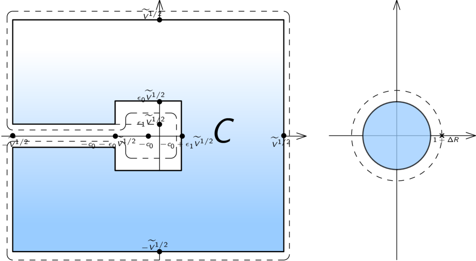
Figure 4: The set ${\mathcal{C}}$ and the image of $\varphi(z)$

Such expression for the inverse function $z=\varphi^{-1}(w)$ is supplied in a version of the Schwarz–Christoffel formula (see [Ahl79, Chapter 6, § 2.2, Theorem 5], [Mar65, Section 47, Theorem 9.9]).

The main fact we need about the Schwarz–Christoffel function $\varphi(z)$ is its asymptotically linear behavior in a neighborhood of $-c_{0}+\varepsilon_{1}\widetilde{V}^{1/2}$, if this point is sufficiently far from the vertices of our polygon.

More precisely, let $\varphi$ be defined in Theorem 8 and $D(-c_{0},\varepsilon_{1}\widetilde{V}^{1/2})$ be the disk of the $z$-plane centered at $-c_{0}$ of radius $\varepsilon_{1}\widetilde{V}^{1/2}$. Then for $\Delta R\asymp\varepsilon_{1}$ with $\varepsilon_{1}$ sufficiently small in comparison with $\varepsilon_{0}$ the set

$$\{z=\varphi^{-1}(w)\ {:}\ |w|=1+\Delta R\}\cap D(-c_{0},\varepsilon_{1}\widetilde{V}^{1/2})$$

lies within $\frac{1}{2}\varepsilon_{1}\widetilde{V}^{1/2}$ of the boundary $\partial{\mathcal{C}}$ in its exterior.

Proof of Theorem 10. Let $p_{n}(z)$ be the polynomial of degree $n$ which coincides with $f(z)$ in the points $\zeta_{1}^{(n+1)},\zeta_{2}^{(n+1)},\dots,\zeta_{n+1}^{(n+1)}$ of Theorem 9. Using [Wal56, § 4.5, Equation (11)] (Hermite’s formula), we have

$$f(z)-p_{n}(z)=\frac{1}{2\pi i}\int\limits_{C_{R}}\frac{\omega_{n+1}(z)f(t)\,dt}{\omega_{n+1}(t)(t-z)},\qquad z\in{\mathcal{C}}.$$

Taking Theorem 9 into account, and recalling

$$f(t)=\frac{\widetilde{\mathcal{M}}}{c_{0}(\alpha)+t},$$

with $\widetilde{\mathcal{M}}\ll\varepsilon_{1}\widetilde{V}^{1/2}$, we see that for $z$ on ${\mathcal{C}}$ we have, with $R_{1}=1+\frac{1}{2}\Delta R$,

$$|f(z)-p_{n}(z)|\ll\frac{n+2}{\varepsilon_{1}^{2}\left(1+\frac{1}{2}\Delta R\right)^{n}},\qquad z\text{ on }{\mathcal{C}}.$$

The above construction needs to be adjusted in order to have the polynomials ${\mathcal{L}}_{n,{\mathcal{C}}}(z)$ with ${\mathcal{L}}_{n,{\mathcal{C}}}(0)=\frac{1}{c_{0}(\alpha)}$. For a sequence of polynomials $p_{n}(z)$ and some shift $z_{0}$ which is independent of $z$ and such that $|z_{0}|\ll\varepsilon_{1}\widetilde{V}^{1/2}$, for $\widetilde{\mathcal{M}}\ll\varepsilon_{1}\widetilde{V}^{1/2}=\alpha^{\varepsilon^{\prime}}$ and for ${\mathcal{L}}_{n,{\mathcal{C}}}(z)=p_{n}(z+z_{0})$ we have ${\mathcal{L}}_{n,{\mathcal{C}}}(0)=\frac{1}{c_{0}(\alpha)}$ which is necessary for Theorem 2 (this condition is essential in the application of Littlewood’s lemma), and

$$\max_{z+z_{0}\in{\mathcal{C}}}\left|\frac{\widetilde{\mathcal{M}}}{c_{0}(\alpha)+z+z_{0}}-{\mathcal{L}}_{n,{\mathcal{C}}}(z)\right|\ll\frac{n+2}{\varepsilon_{1}^{2}\left(1+\frac{1}{2}\Delta R\right)^{n}}$$ (23)

with the absolute implied constant.

10 Completion of proof of Theorem 1

Let in Theorem 2

$$a=\frac{1}{2}-\frac{R-\delta_{T}}{\log T}$$

with

$$R=\varepsilon\log\alpha,$$

$\varepsilon>0$ fixed, and let

$$\Delta\sigma=\frac{\alpha}{\log T},$$

where $\alpha>0$ is real and goes to infinity with $T$ sufficiently slowly.

Recall that in (23) $\widetilde{\mathcal{M}}$ is such that

$$\widetilde{\mathcal{M}}\ll\varepsilon_{1}\widetilde{V}^{1/2}=\alpha^{\varepsilon^{\prime}},$$

and in the proof of Theorem 5 we established that we can take

$$\widetilde{V}^{1/2}=\alpha^{C(1/2-2\varepsilon)}$$

with large fixed $C>0$.

We take $\varepsilon>0$ so that $\frac{\varepsilon^{\prime}}{\varepsilon}$ is arbitrarily small.

Using Theorems 3, 4, 5, and denoting $E=E_{\alpha,\delta_{T}}\cup([T,2T]\setminus{\mathcal{M}}_{\alpha})$ we can write

$$\begin{split}\frac{2}{R}\log I(R)&=\frac{2}{R}\log\left(\frac{1}{T-\varepsilon_{E}T}\int\limits_{[T,2T]\setminus E}|F^{\ast}(a+it)|\,dt\right)\\ &=\frac{2}{R}\log\left(\frac{1}{T-\varepsilon_{E}T}\int\limits_{[T,2T]\setminus E}|\zeta(a+\Delta\sigma+it)||c_{0}(\alpha)+\lambda(a+\Delta\sigma+it)|\right.\\ &\left.\vphantom{\int\limits_{[T,2T]\setminus E}\zeta}\times|M(a+it)||{\mathcal{L}}(A(a+\Delta\sigma+it))|\,dt\right),\end{split}$$

and

$$\begin{split}&\bigg{|}c_{0}(\alpha)+\lambda(a+\Delta\sigma+it)\bigg{|}|{\mathcal{L}}(A(a+\Delta\sigma+it))|\\ &\ll\widetilde{\mathcal{M}}+\frac{\left|c_{0}(\alpha)+A(a+\Delta\sigma+it)\right|}{\widetilde{V}^{10}}\end{split}$$

by (16) and (23), since we chose $n\asymp\frac{1}{\varepsilon_{1}}\log\left(\frac{\widetilde{V}^{1/2}}{\varepsilon_{1}}\right)$ and

$$\max\limits_{t\in[T,2T]\setminus E}\left|\frac{\widetilde{\mathcal{M}}}{c_{0}+A(s)}-{\mathcal{L}}(A(s))\right|\ll\frac{1}{\widetilde{V}^{10}}.$$

We have $\frac{\log\widetilde{\mathcal{M}}}{R}$ arbitrarily small. Now we apply the Cauchy–Schwarz inequality and show that for

$$\bar{R}=\alpha-R+\delta(T)>0$$

we have

$$\int\limits_{T}^{2T}|\zeta(\frac{1}{2}+\frac{\bar{R}}{\log T}+it)|^{2}|M(a+it)|^{2}\,dt\leqslant(1+\varepsilon(\alpha,T))T$$

with $\varepsilon(\alpha,T)>0$ arbitrarily small.

To prove the estimate, in [Con89, Theorem 2] we take $R=-\bar{R}$ (note that our $\bar{R}>0$, but $R$ can be negative in Conrey’s theorem), $Q(x)=1$, and take $0<\theta<\frac{4}{7}$ so that $\theta\bar{R}$ goes to infinity with $\alpha$. Then Conrey’s theorem asserts that for an optimal choice of $P$ in the mollifier $M(s)$ we have (see [Con89, (49)])

$$\int\limits_{T}^{2T}|\zeta(\frac{1}{2}+\frac{\bar{R}}{\log T}+it)|^{2}|M(a+it)|^{2}\,dt\thicksim c(1,\bar{R})T,$$

with

$$c(1,\bar{R})=\frac{1}{2}\left(|w(0)|^{2}+|w(1)|^{2}\right)+A\bar{\alpha}\frac{\coth\bar{\alpha}}{\theta}.$$

Here

$$w(y)=\exp(-\bar{R}y),$$

$$A=\int\limits_{0}^{1}e^{-2\bar{R}y}dy,$$

$$\bar{\alpha}=\sqrt{\frac{C}{A}},$$

$$C=\theta^{2}\int\limits_{0}^{1}{\bar{R}}^{2}e^{-2\bar{R}y}dy,$$

i. e.

$$c(1,\bar{R})=\frac{1}{2}+\frac{1}{2}|w(1)|^{2}+\sqrt{A\frac{C}{\theta^{2}}}\coth\bar{\alpha}.$$

We have

$$w(1)=e^{-\bar{R}},$$

$$A=\frac{1}{2\bar{R}}\left(1-e^{-2\bar{R}}\right),$$

$$\frac{C}{\theta^{2}}=\frac{\bar{R}}{2}\left(1-e^{-2\bar{R}}\right),$$

$$A\frac{C}{\theta^{2}}=\frac{1}{4}\left(1-e^{-2\bar{R}}\right)^{2},$$

$$\bar{\alpha}=\theta\bar{R}.$$

Thus, if $\bar{R}$ can be taken arbitrarily large, then $c(1,\bar{R})\leqslant(1+\varepsilon(\bar{R}))$, with $\varepsilon(\bar{R})$ arbitrarily small.

The remaining terms in Theorem 2 are small by Theorem 5.

This completes the proof of Theorem 1.

References

• [Ahl79] L. V. Ahlfors, Complex Analysis, McGraw-Hill, Inc., Third Edition, 1979.
• [Con83] J. B. Conrey, Zeros of derivatives of the Riemann’s $\xi$-function on the critical line, J. Number Theory 16 (1983), 49–74.
• [Con89] J. B. Conrey, More than two fifths of the zeros of the Riemann zeta function are on the critical line, J. reine angew. Math. 399 (1989), 1–26.
• [Fen12] S. Feng, Zeros of the Riemann zeta function on the critical line, J. Number Theory 132 (2012), 511–542.
• [Gai87] D. Gaier, Lectures on Complex Approximation. BirkhΓ€user, Boston, 1987.
• [H14] G. H. Hardy, Sur les zΓ©ros de la fonction ΢​(s)πœπ‘ \zeta(s) de Riemann, C. R. 158 (1914), 1012–1014.
• [HL21] G. H. Hardy and J. E. Littlewood, The zeros of Riemann’s zeta-function on the critical line, Math. Z. 10 (1921), 283–317.
• [Iw14] H. Iwaniec, Lectures on the Riemann Zeta Function, volume 62 of University Lecture Series. American Mathematical Society, 2014.
• [Jut82] M. Jutila, Zeros of the zeta-function near the critical line, Studies in pure mathematics, to the memory of Paul TurΓ‘n, BirkhaΓΌser (1982), 385–394.
• [Ki11] H. Ki, Zeros of zeta functions, Comment. Math. Univ. St. Pauli 60(1–2) (2011) 99–117.
• [Les13a] S. J. Lester, The distribution of the logarithmic derivative of the Riemann zeta-function. arXiv:1308.3597 [math.NT].
• [Les13b] S. J. Lester, The Distribution of Values of the Riemann Zeta-Function, Thesis. University of Rochester, Rochester, New York, 2013.
• [Lev74] N. Levinson, More than one third of zeros of Riemann’s zeta-function are on $\sigma=\frac{1}{2}$, Adv. Math. 13 (1974), 383–436.
• [Mar65] A. I. Markushevich, Theory of Functions of a Complex Variable, Vol.Β 3, Prentice-Hall, Englewood Cliffs, 1965.
• [Sel42] A. Selberg, On the zeros of Riemann’s zeta-function, Skr. Norske Vid. Akad. Oslo 10 (1942), 1–59.
• [Sel46] A. Selberg, Contributions to the theory of the Riemann zeta-function, Arch. Math. Naturvid. 48 (1946) no. 5, 89–155.
• [Sz75] G. SzegΓΆ, Orthogonal polynomials, volume XXIII of AMS Colloquium Publications. American Mathematical Society, Fourth Edition, 1975.
• [Tsang84] K.-M. Tsang, The Distribution of the Values of the Riemann Zeta-Function, Thesis. Princeton University, Princeton, October 1984.
• [Wal56] J. Walsh, Interpolation and Approximation by Rational Functions in the Complex Domain, volume XX of AMS Colloquium Publications. American Mathematical Society, Second Edition, 1956.