Abstract

We investigate anisotropic compact stars in the non-minimal $Y(R)F^{2}$ model of gravity which couples an arbitrary function of curvature scalar $Y(R)$ to the electromagnetic field invariant $F^{2}$. After we obtain exact anisotropic solutions to the field equations of the model, we apply the continuity conditions to the solutions at the boundary of the star. Then we find the mass, electric charge, and surface gravitational redshift by the parameters of the model and radius of the star.

I Introduction

Compact stars are the best sources to test a theory of gravity under the extreme cases with strong fields. Although they are generally considered as isotropic, there are important reasons to take into account anisotropic compact stars which have different radial and tangential pressures. First of all, the anisotropic spherically symmetric compact stars can be more stable than the isotropic ones Dev . The core region of the compact stars with very high nuclear matter density becomes more realistic in the presence of anisotropic pressures Ruderman ; Canuto . Moreover the phase transitions Sokolov , pion condensations Sawyer and the type 3A superfluids Kippenhahm in the cooling neutron matter core can lead to anisotropic pressure distribution. Furthermore, the mixture of two perfect fluid can generate anisotropic fluid Letelier . Anisotropy can be also sourced by the rotation of the star Herrera ; Bayin ; Silva . Additionally, strong magnetic fields may lead to anisotropic pressure components in the compact starsMak2002 . Some analytic solutions of anisotropic matter distribution were studied in Einsteinian Gravity Herrera ; Bayin ; Silva ; Mak2002 ; Delgaty ; Harko2002 ; Mak2003 ; Bowers ; Mak20022 ; Durgapal1985 . Recently it was shown that the ”scalarization” can not arise without anisotropy and the anisotropy range can be determined by observations on binary pulsar in the Scalar-Tensor Gravity and General Relativity Silva . The anisotropic star solutions in $R^{2}$ gravity can shift the mass-radius curves to the region given by observations Folomeev . It is interesting to note that anisotropic compact stars were investigated in Rastall theory and found exact solutions which permit the formation of super-massive star Salako2018 .

Additionally, the presence of a constant electric charge on the surface of compact stars may increase the stability Stettner and protect them from collapsing Krasinski ; Sharma . The charged fluids can be described by the minimally coupled Einstein-Maxwell field equations. An exact isotropic solution of the Einstein-Maxwell theory were found by Mak and Harko describing physical parameters of a quark star with the MIT bag equation of state under the existence of conformal motions mak-harko-2004 . Also, the upper and lower limits for the basic physical quantities such as mass-radius ratio, redshift were derived for charged compact stars Mak2001 and for anisotropic stars Bohmer2006 . A regular charged solution of the field equations which satisfy physical conditions was found in Krori and the constants of the solution were fixed in terms of mass, charge and radius Junevicus . Later the solutions were extended to the charged anisotropic fluids Varela ; Rahaman . Also, anisotropic charged fluid spheres were studied in $D$-dimensions Harko2000 .

In the investigation of compact stars, one of the most important problem is the mass discrepancy between the predictions of nuclear theories Xu2010 ; Glendenning1991 ; Panda2004 ; Page2006 and neutron star observations. The resent observations such as $1.97M_{\odot}$ of the neutron star PSR J1614-2230 Demorest2010 , $2.4M_{\odot}$ of the neutron stars B1957+20 Kerkwijk2011 and 4U 1700-377 Clark2002 or $2.7M_{\odot}$ of J1748-2021B Freire2008 can not be explained by using any soft equation of state in Einstein’s gravity Xu2010 ; Demorest2010 ; Wen2012 . Since each different approach which solves this problem leads to different maximal mass, we need to more reliable models which satisfy observations and give the correct maximum mass limit of compact stars.

On the other hand, the observational problems such as dark energy and dark matter Overduin ; Baer ; Riess ; Perlmutter ; Knop ; Amanullah ; Weinberg ; Schwarz at astrophysical scales have caused to search new modified theories of gravitation such as $f(R)$ gravity Capozz2011 ; Nojiri2011 ; Nojiri2007 ; Capozz2010 ; Capozz2003 ; Joyce ; Capozz2012 . As an alternative approach, the $f(R)$ theories of gravitation can explain the inflation and cosmic acceleration without exotic fields and satisfy the cosmological observations Nojiri2003 ; Nojiri20032 . Therefore, in the strong gravity regimes such as inside the compact stars, $f(R)$ gravity models can be considered to describe the more massive stars Capozziello2016 ; Astashenok2014 . Furthermore, the strong magnetic fields Astashenok2015 and electric fields Jing2015 can increase the mass of neutron stars in the framework of $f(R)$ gravity.

On the other hand, in the presence of the strong electromagnetic fields, the Einstein-Maxwell theory can also be modified. The first modification is the minimal coupling between $f(R)$ gravity and Maxwell field as the $f(R)-$Maxwell gravity which has only the spherically symmetric static solution Dombriz2009 . Therefore we consider the more general modifications such as $Y(R)F_{ab}F^{ab}$ which allow a wide range of solutions AADS ; dereli3 ; Sert12Plus ; Sert13MPLA ; bamba1 ; bamba2 ; Sert-Adak12 ; dereli4 ; Turner ; Mazzi ; Campa .

A similar kind of such a modification which is $R_{abcd}F^{ab}F^{cd}$ firstly was defined by Prasanna Prasanna and found a criterion for null electromagnetic fields in conformally flat space-times. Then the most general possible invariants which involves electromagnetic and gravitational fields (vector-tensor fields) including $RF_{ab}F^{ab}$ term were studied in Horndeski and the spherically symmetric static solutions were obtained Muller-Hoissen1988 for the unique composition of such couplings. Also such non-minimal modifications were derived by dimensional reduction of the five dimensional Gauss-Bonnet action Muller-Hoissen1988-2 ; Muller-Hoissen1988-3 and $R^{2}$ gravity action Buchdahl1979 ; Dereli1990 . These invariant terms were also obtained by Feynman diagram method from vacuum polarization of the photon in the weak gravitational field limit Drummond1980 . The general form of the couplings such as $R^{n}F^{2}$ were used to explain the seed magnetic fields in the inflation and the production of the primeval magnetic flux in the universe Turner ; Campa ; Kunze ; Mazzi ; dereli4 ; bamba1 .

Thus it is natural to consider the more general modifications which couple a function of the Ricci scalar with Maxwell invariant as $Y(R)F^{2}$ form inside the strong electromagnetic and gravitational fields such as compact astrophysical objects. The more general modifications have static spherically symmetric solutions Sert12Plus ; dereli3 ; dereli4 ; Sert13MPLA to describe the flatness of velocity curves of galaxies, cosmological solutions to describe accelerating expansion of the universe Sert-Adak12 ; AADS ; bamba1 ; bamba2 and regular black hole solutions Sert2016regular . Furthermore, the charged, isotropic stars and radiation fluid stars can be described by the non-minimal couplings Sert2017 ; Sert2018 . Therefore in this study, we investigate the anisotropic compact stars in the non-minimal $Y(R)F^{2}$ model and find a family of exact analytical solutions. Then we obtain the total mass, total charge and gravitational surface redshift by the parameters of the model and the boundary radius of the star.

II The Model for Anisotropic Stars

We will obtain the field equations of our model for the anisotropic stars by varying the action integral with respect to independent variables; the orthonormal co-frame 1-form $e^{a}$, the Levi-Civita connection 1-form $\omega_{ab}$, and the electromagnetic potential 1- form $A$,

$$I=\int_{M}{\left\{\frac{1}{2\kappa}R*1-\epsilon_{0}Y(R)F\wedge*F+\frac{2}{c}A\wedge J+L_{mat}+\lambda_{a}\wedge T^{a}\right\}}$$ (1)

where $\kappa$ is the coupling constant, $\epsilon_{0}$ is the permittivity of free space, $\wedge$ and $*$ denote the exterior product and the Hodge map of the exterior algebra, respectively, $R$ is the curvature scalar, $Y(R)$ is a function of $R$ representing the non-minimal coupling between gravity and electromagnetism, $F$ is the electromagnetic 2-form, $F=dA$, $J$ is the electromagnetic current 3-form, $L_{mat}$ is the matter Lagrangian 4-form, $T^{a}:=de^{a}+\omega^{a}{}_{b}\wedge e^{b}$ is the torsion 2-form, $\lambda_{a}$ Lagrange multiplier 2-form constraining torsion to zero and $M$ is the differentiable four-dimensional manifold whose orientation is set by the choice $*1=e^{0}\wedge e^{1}\wedge e^{2}\wedge e^{3}$.

In this study, we use the SI units differently from the previous papers Sert2017 ; Sert2018 . We write $F=-E_{i}e^{0i}+\frac{c}{2}\epsilon_{0ijk}B^{k}e^{ij}$, where $c$ is the light velocity, $E_{i}$ is electric field and $B_{i}$ is magnetic field under the assumption of the Levi-Civita symbol $\epsilon_{0123}=+1$. We adhere the following convention about the indices; $a,b,c=0,1,2,3$ and $i,j,k=1,2,3$. We also define $J=-c\rho_{e}*e^{0}+J_{i}*e^{i}$ where $\rho_{e}$ is the charge density and $J_{i}$ is the current density. We assume that the co-frame variation of the matter sector of the Lagrangian produces the following energy momentum 3-form

$$\tau_{a}^{mat}:=\frac{\partial L_{mat}}{\partial e^{a}}=(\rho c^{2}+p_{t})u_{a}*u+p_{t}*e_{a}+(p_{r}-p_{t})v_{a}*v$$ (2)

where $u=\delta_{a}^{0}e^{a}$ is a time-like 1-form, $v=\delta_{a}^{1}e^{a}$ is a space-like 1-form, $p_{r}$ is the radial component of pressure orthogonal to the transversal pressure $p_{t}$, and $\rho$ is the mass density for the anisotropic matter in the star. In this case it must be $\kappa=8\pi G/c^{4}$ for the correct Newton limit. The non-minimal coupling function $Y(R)$ is dimensionless. Consequently every term in our Lagrangian has the dimension of $(energy)(length)$. Finally we notice that the dimension of $\lambda_{a}$ must be $energy$ because torsion has the dimension of $length$.

After substituting the connection varied equation into the co-frame varied one, we obtain the modified Einstein equation for our model

$$-\frac{1}{2\kappa}R^{bc}\wedge*e_{abc} = \epsilon_{0}Y(\iota_{a}F\wedge*F-F\wedge\iota_{a}*F)+\epsilon_{0}Y_{R}F_{bc}F^{bc}*R_{a}$$ (3)

$$+\epsilon_{0}D[\iota^{b}\;d(Y_{R}F_{bc}F^{bc})]\wedge*e_{ab}+\tau_{a}^{mat}\ ,\hskip 28.45274pt$$

where $\iota$ denotes the interior product of the exterior algebra satisfying the duality relation, $\iota_{b}e^{a}=\delta^{a}_{b}$, through the Kronecker delta, $R^{a}{}_{b}:=d\omega^{a}{}_{b}+\omega^{a}{}_{c}\wedge\omega^{c}{}_{b}$ is the Riemann curvature 2-form, $R^{a}:=\iota_{b}R^{ba}$ is the Ricci curvature 1-form, $R:=\iota_{a}R^{a}$ is the curvature scalar, $Y_{R}:=dY/dR$, $e^{ab\cdots}:=e^{a}\wedge e^{b}\wedge\cdots$ and $F_{bc}:=\iota_{c}\iota_{b}F$. As the left hand side of the equation (3) constitutes the Einstein tensor, the right one is called the total energy momentum tensor for which the law of energy-momentum conservation is valid. For details one may consult Ref. Sert2017 .

The variation of the action according to the electromagnetic potential $A$ yields the modified Maxwell equation

$$\epsilon_{0}d(*YF) = \frac{J}{c}\;.$$ (4)

We have also noticed that the Maxwell 2-form is closed $dF=0$ from the Poincaré lemma, since it is exact form $F=dA$. Thus, the two field equations (3) and (4) define our model and we will look for solutions to them under the condition

$$\epsilon_{0}Y_{R}F_{bc}F^{bc}=-\frac{k}{\kappa}$$ (5)

which removes the potential instabilities from the higher order derivatives for the non-minimal theory. Here the non-zero $k$ is a dimensionless constant. The case of $k=0$ leads to $Y(R)=constant$ corresponding to the minimal Einstein-Maxwell theory which will be considered as the exterior vacuum solution with $R=0$. We will see from solutions of the model that the total mass and total charge of the anisotropic star are critically dependent on the parameter $k$. The additional features of the constraint (5) may be found in Sert2017 . We also notice that the trace of the modified Einstein equation (3), obtained by multiplying with $e^{a}\wedge$, produces an explicit relation between the Ricci curvature scalar, energy density and pressures

$$(1-k)R=\kappa(\rho c^{2}-p_{r}-2p_{t})\;.$$ (6)

III Static spherically symmetric Anisotropic solutions

We propose the following metric for the static spherically symmetric spacetime and the Maxwell 2-form for the static electric field parallel to radial coordinate in (1+3) dimensions

$$ds^{2} = -f^{2}(r)c^{2}dt^{2}+g^{2}(r)dr^{2}+r^{2}d\theta^{2}+r^{2}\sin^{2}\theta d\phi^{2}\;,$$ (7)

$$F = E(r)e^{1}\wedge e^{0}\;,$$ (8)

where $f$ and $g$ are the metric functions and $E$ is the electric field in the radial direction which all three functions depend only on the radial coordinate $r$.

The integral of the electric current density 3-form $J$ sourcing the electric field gives rise to the electric charge inside the volume $V$ surrounded by the closed spherical surface $\partial V$ with radius $r$

$$q(r):=\frac{1}{c}\int_{V}{J}=\epsilon_{0}\int_{V}{d(*YF)}=\epsilon_{0}\int_{\partial V}{*YF}=4\pi\epsilon_{0}r^{2}YE\,.$$ (9)

Here we used the Stoke’s theorem. The components of the modified Einstein equation (3) reads three coupled nonlinear differential equations

$$\frac{1}{\kappa}\left(\frac{2g^{\prime}}{g^{3}r}+\frac{g^{2}-1}{g^{2}r^{2}}\right)=\epsilon_{0}YE^{2}-\frac{k}{\kappa}\left(\frac{f^{\prime\prime}}{fg^{2}}-\frac{f^{\prime}g^{\prime}}{fg^{3}}+\frac{2f^{\prime}}{fg^{2}r}\right)+\rho c^{2}\;,$$ (10)

$$\frac{1}{\kappa}\left(-\frac{2f^{\prime}}{fg^{2}r}+\frac{g^{2}-1}{g^{2}r^{2}}\right)=\epsilon_{0}YE^{2}+\frac{k}{\kappa}\left(-\frac{f^{\prime\prime}}{fg^{2}}+\frac{f^{\prime}g^{\prime}}{fg^{3}}+\frac{2g^{\prime}}{g^{3}r}\right)-p_{r}\;,$$ (11)

$$\frac{1}{\kappa}\left(\frac{f^{\prime\prime}}{fg^{2}}-\frac{f^{\prime}g^{\prime}}{fg^{3}}+\frac{f^{\prime}}{fg^{2}r}-\frac{g^{\prime}}{g^{3}r}\right)=\epsilon_{0}YE^{2}-\frac{k}{\kappa}\left(-\frac{f^{\prime}}{fg^{2}r}+\frac{g^{\prime}}{g^{3}r}+\frac{g^{2}-1}{g^{2}r^{2}}\right)+p_{t}\;,$$ (12)

where prime stands for derivative with respect to $r$. We obtain one more useful equation by taking the covariant exterior derivative of (3)

$$p_{r}^{\prime}+\frac{f^{\prime}(\rho c^{2}+p_{r})}{f}+\frac{2(p_{r}-p_{t})}{r}=2\epsilon_{0}(YE)^{\prime}E+\frac{4\epsilon_{0}YE^{2}}{r}\,.$$ (13)

In what follows we assume the linear equation of state in the star

$$p_{r}=\omega\rho c^{2}$$ (14)

where $\omega$ is a constant in the interval $0<\omega\leq 1$. Finally we calculate the crucial constraint (5)

$$\frac{dY}{dR}=\frac{k}{2\epsilon_{0}\kappa E^{2}}\;,$$ (15)

where the Ricci curvature scalar is

$$R=\frac{2}{g^{2}}\left(-\frac{f^{\prime\prime}}{f}+\frac{f^{\prime}g^{\prime}}{fg}-\frac{2f^{\prime}}{fr}+\frac{2g^{\prime}}{gr}+\frac{g^{2}-1}{r^{2}}\right)\;.$$ (16)

III.1 Exact solutions with conformal symmetry

We will look for solutions to these differential equations (10)-(15) assuming that the metric (7) admits a one-parameter group of conformal motions, since inside of stars can be described by using this symmetry mak-harko-2004 ; Herrera1 ; Herrera2 ; Herrera3 . The symmetry is obtained by taking Lie derivative of the metric tensor $\mathbf{g}_{ab}$ with respect to the vector field $\xi$, $L_{\xi}\mathbf{g}_{ab}=\frac{\phi_{0}}{g(r)}\mathbf{g}_{ab}$, for the arbitrary metric function $g(r)$ and the following metric function $f(r)$

$$f^{2}(r)=a^{2}r^{2}$$ (17)

with arbitrary constants $a$ and $\phi_{0}$. Here we consider the metric function $g(r)$

$$g^{2}(r)=\frac{3}{1+br^{\alpha}}\;,$$ (18)

inspired by mak-harko-2004 , where $b$ and $\alpha$ are arbitrary parameters. With these choices, the curvature scalar (16) is calculated as

$$R=-b(\alpha+2)r^{\alpha-2}\,.$$ (19)

We notice that it must be $\alpha>2$ and $b\neq 0$ in order for that the curvature scalar is nonzero and regular at the origin. If $b=0$, then the curvature scalar $R$ becomes zero and this leads to constant $Y(R)$ in which case the model reduces to the minimal Einstein-Maxwell theory.

Then the system of equations (10)-(15) has the following solutions for the metric functions (17), (18) and the anisotropic pressure $p_{r}=\omega\rho c^{2}$

$$\rho(r)=\frac{(k+1)[2-br^{\alpha}(\alpha-2)]}{3\kappa c^{2}r^{2}(\omega+1)}\,,$$ (20)

(21)

$$p_{t}(r)=\frac{br^{\alpha}[(k+1)(\alpha-2)-X]}{3\kappa r^{2}(\omega+1)}+\frac{(k+1)(1-\omega)}{3\kappa r^{2}(\omega+1)}\,,$$ (22)

$$E^{2}(r)=\frac{2\omega(k+1)}{3\kappa\epsilon_{0}c_{0}r^{2}(\omega+1)}\left[1+\frac{Xbr^{\alpha}}{4\omega(k+1)}\right]^{1+\frac{3k(\omega+1)(\alpha^{2}-4)}{\alpha X}}\,,$$ (23)

$$Y(r)=c_{0}\left[1+\frac{Xbr^{\alpha}}{4\omega(k+1)}\right]^{-\frac{3k(\omega+1)(\alpha^{2}-4)}{\alpha X}}\,,$$ (24)

where the composite function $Y(R(r))$ have obtained in terms of $r$ as $Y(r)$ and we have defined

$$X=k\omega(\alpha+4)+\alpha(3k-2\omega)-2(\omega+3)\,.$$ (25)

After obtaining $r(R)$ from (19)

$$r=\left[\frac{-R}{b(\alpha+2)}\right]^{1/(\alpha-2)}$$ (26)

we rewrite explicitly the non-minimal coupling function in terms of $R$

$$Y(R)=c_{0}\left[1+\frac{bX}{4\omega(k+1)}\left(\frac{-R}{\alpha b+2b}\right)^{\alpha/(\alpha-2)}\right]^{-\frac{3k(\omega+1)(\alpha^{2}-4)}{\alpha X}}.$$ (27)

Since the exterior vacuum region is described by Reissner-Nordström metric satisfying $R=0$, the non-minimal coupling function becomes $Y(R)=c_{0}$. Therefore we can fix $c_{0}=1$ without loss of generality. Then the corresponding model becomes

$$L=\frac{1}{2\kappa^{2}}R*1-\epsilon_{0}\left[1+\frac{bX}{4\omega(k+1)}\left(\frac{-R}{(\alpha+2)b}\right)^{\frac{\alpha}{\alpha-2}}\right]^{-\frac{3k(\omega+1)(\alpha^{2}-4)}{\alpha X}}\hskip-19.91684ptF\wedge*F+2A\wedge J+L_{mat}+\lambda_{a}\wedge T^{a}.\ \ \ \ \ \$$ (28)

admitting the interior metric

$$ds^{2}_{in}=-a^{2}r^{2}c^{2}dt^{2}+\frac{3}{1+br^{\alpha}}dr^{2}+r^{2}d\Omega^{2}\;$$ (29)

and the the Maxwell 2-form

$$F=\frac{q(r)}{4\pi\epsilon_{0}Yr^{2}}e^{1}\wedge e^{0}$$ (30)

in the interior of star, where $q(r)$ is obtained from (9) as

$$q^{2}(r)=\frac{32\pi^{2}\epsilon_{0}\omega(k+1)r^{2}}{3\kappa(\omega+1)}\left[1+\frac{Xbr^{\alpha}}{4\omega(k+1)}\right]^{1-\frac{3k(\omega+1)(\alpha^{2}-4)}{\alpha X}}\,.$$ (31)

On the other hand at the exterior, the model admit the Reissner-Nordström metric

$$ds^{2}_{out}=-\left(1-\frac{2GM}{c^{2}r}+\frac{\kappa Q^{2}}{(4\pi)^{2}\epsilon_{0}r^{2}}\right)c^{2}dt^{2}+\left(1-\frac{2GM}{c^{2}r}+\frac{\kappa Q^{2}}{(4\pi)^{2}\epsilon_{0}r^{2}}\right)^{-1}dr^{2}+r^{2}d\Omega^{2}\;$$ (32)

and the Maxwell 2-form

$$F=\frac{Q}{4\pi\epsilon_{0}r^{2}}e^{1}\wedge e^{0}$$ (33)

which represents the electric field in the radial direction, $\vec{E}={\hat{r}Q}/{4\pi\epsilon_{0}r^{2}}$, where $Q$ is the total electric charge of the star which is obtained by writing $r=r_{b}$ in (31). We will be able to determine some of the parameters from the matching and the continuity conditions, and the others from the observational data.

III.2 Matching conditions

We will match the interior metric (29) and the exterior metric (32) at the boundary of the star $r=r_{b}$ for continuity of the gravitational potential,

$$a^{2}r_{b}^{2} = 1-\frac{2GM}{c^{2}r_{b}}+\frac{\kappa Q^{2}}{(4\pi)^{2}\epsilon_{0}r_{b}^{2}}\,,$$ (34)

$$\frac{3}{1+br^{\alpha}_{b}} = \left(1-\frac{2GM}{c^{2}r_{b}}+\frac{\kappa Q^{2}}{(4\pi)^{2}\epsilon_{0}r_{b}^{2}}\right)^{-1}\,.$$ (35)

These equations are solved for $a$ and $b$ appeared in the interior metric functions

$$b=\frac{2r_{b}^{2}-6GMr_{b}/c^{2}+3\kappa Q^{2}/(4\pi)^{2}\epsilon_{0}}{r_{b}^{2+\alpha}}\,,$$ (36)

$$a^{2}=\frac{1}{r_{b}^{2}}-\frac{2GM}{c^{2}r_{b}^{3}}+\frac{\kappa Q^{2}}{(4\pi)^{2}\epsilon_{0}r_{b}^{4}}\,.$$ (37)

Vanishing of the radial pressure at the boundary, $p_{r}(r_{b})=\omega c^{2}\rho(r_{b})=0$ in (20), determines the parameter $b$

$$b=\frac{2}{(\alpha-2)r_{b}^{\alpha}}\;.$$ (38)

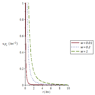
(a) $p_{r}(r)$

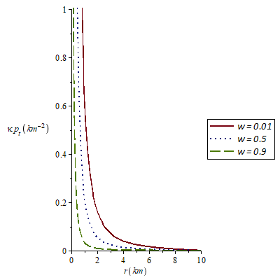
(b) $p_{t}(r)$

Figure 1: The radial (a) and tangential (b) pressures as a function of the radial distance $r$ for $k=1$, $\alpha=4$, $r_{b}=10km$ and some different $\omega$ values. (The energy density $c^{2}\rho$ is proportional to the radial pressure as $p_{r}=\omega c^{2}\rho$ )

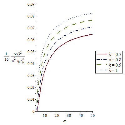
(a) $\omega=0.1$

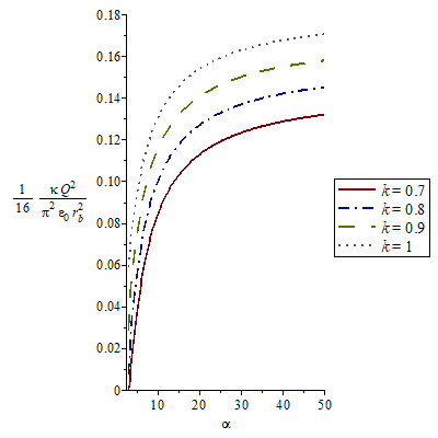
(b) $\omega=0.3$

Figure 2: The dimensionless quantity which is related with the total charge $Q$ as a function of the parameter $\alpha$ for $\omega=0.1$(a) and $\omega=0.3$ (b).

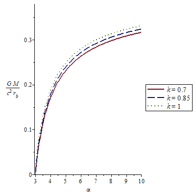
(a) $\omega=0.15$

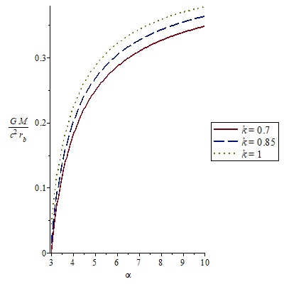
(b) $\omega=0.5$

Figure 3: The dimensionless quantity related with the total mass as a function of $\alpha$ for $\omega=0.15$ (a) and $\omega=0.5$ (b).

The behavior of the pressures and energy density is given in Fig. 1 in terms of the radial distance $r$ for $k=1$. Moreover the decreasing behavior of the quantities does not change for $k\neq 1$. We can obtain an upper bound of the parameter $k$ using the non-negative tangential pressure $p_{t}(r)$ in (22). In order to obtain the bound we need to determine the interval of $\omega$. Since the radial component of the sound velocity $\frac{dp_{r}}{d\rho}$ is non-negative and should not be bigger than the square of light velocity $c^{2}$ for the normal matter, the parameter $\omega$ takes values in the range $0\leq\omega\leq 1$. We see from the Fig. 1b that the tangential pressure curves decrease for the increasing $\omega$ values and the minimum curve can be obtained from the case with $\omega=1$. Then we obtain the following inequality from the first part of $p_{t}(r)$

$$(k+1)(\alpha-2)-X\geq 0$$ (39)

which turns out to be

$$3(1-k)(\alpha+2)\geq 0$$ (40)

for the case $\omega=1$, that leads to the minimum $p_{t}(r)$ function. Thus the parameter $k$ must be $k\leq 1$ for the non-negative tangential pressure. On the other hand, the total electric charge (43) must be a real valued exponential function, then we obtain the inequality

$$1+\frac{2X}{4\omega(k+1)(\alpha-2)}\geq 0$$ (41)

which leads to $k\geq\frac{2}{\alpha}$. Thus $k$ must take values in this range

$$\frac{2}{\alpha}<k\leq 1.$$ (42)

and we find the maximum lower bound for the parameter $k$ as $k>\frac{2}{3}$ for $\alpha>3$ (which leads to positive gravitational redshift).

While the interior side of the star has the electrically charged matter distribution, the outer side is vacuity. Then the excitation 2-form $\mathcal{G}=YF$ in the interior becomes the Maxwell 2-form $\mathcal{G}=F$ at the exterior. Therefore the interior electric charge $q(r)$ which found from $\epsilon_{0}cd*YF=J$ must be equal to the total electric charge $Q$ obtained from $d*F=0$ at the exterior. Thus the continuity of the excitation 2-form at the boundary leads to $q(r_{b})=Q$ as the last matching condition

$$Q^{2}=\frac{32\pi^{2}\epsilon_{0}\omega(k+1)r_{b}^{2}}{3\kappa(\omega+1)}\left[1+\frac{2X}{4\omega(k+1)(\alpha-2)}\right]^{1-\frac{3k(\omega+1)(\alpha^{2}-4)}{\alpha X}}$$ (43)

where we eliminated the parameter $b$ via (38). The total electric charge is shown as a function of $\alpha$ in Fig. 2 for $\omega=0.1$ (a) and $\omega=0.3$ (b) taking some different $k$ values. We see that the increasing $k$ values increase the total charge values. The substitution of (38) to (36) allows us writing the total mass of the star in terms of its total charge

$$M=\left(\frac{\alpha-3}{\alpha-2}\right)\frac{c^{2}r_{b}}{3G}+\frac{\kappa c^{2}Q^{2}}{2(4\pi)^{2}\epsilon_{0}Gr_{b}}\,.$$ (44)

Then from (43) the total mass becomes

$$M=\left(\frac{\alpha-3}{\alpha-2}\right)\frac{c^{2}r_{b}}{3G}+\frac{c^{2}r_{b}\omega(k+1)}{3G(\omega+1)}\left[1+\frac{2X}{4\omega(k+1)(\alpha-2)}\right]^{1-\frac{3k(\omega+1)(\alpha^{2}-4)}{\alpha X}}.$$ (45)

We depict the graph of the total mass as a function of $\alpha$ in Fig. 3 for $\omega=0.15$ (a) and $\omega=0.5$ (b) taking some different $k$ values.

Additionally, the gravitational surface redshift defined by $z:=\frac{1}{f(r_{b})}-1$ is calculated as

$$z=\sqrt{\frac{3(\alpha-2)}{\alpha}}-1\;.$$ (46)

We see that the gravitational redshift is independent of the parameters $\omega$ and $k$ then the limit $\alpha\to\infty$ gives the upper bound for the redshift, $z<0.732$. On the other hand, $\alpha=3$ gives $z=0$. Then $\alpha$ must be $\alpha>3$ for the observational requirements. Variation of the surface redshift is shown in Fig. 4.

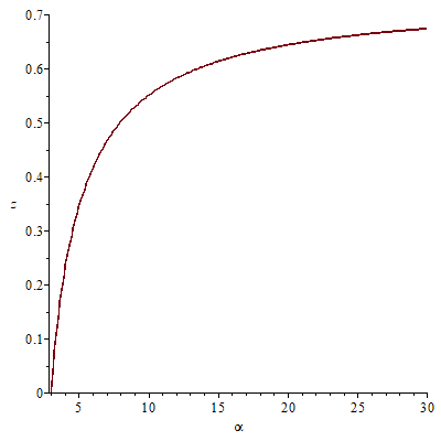
Figure 4: The gravitational surface redshift versus the parameter $\alpha$.

In this model, we see that $\alpha$ can be fixed by the gravitational surface redshift observations due to (46). However, the gravitational redshift measurements do not have enough precise results Cottam2002 ; Lin2010 . Moreover, the observational value of the mass-radius ratio determines one of the two parameters $\omega$ and $k$ from (45). If we can also predict the total charge of star, we can fix $\omega$ and $k$ separately from (43). For example, when we take the gravitational redshift of the neutron star EXO 0748-676 as $z=0.35$ with $M=2M_{\odot}$ and $R=13.1km$ Lin2010 , we find that $\alpha\approx 5.08$ from (46) and there is one free parameter $k$ or $\omega$ that must be fixed in (45). Then we can fix $k=1$ which leads to $\omega\approx 0.01$.

III.3 The Simple Model with $\alpha=4$

The model simplifies for $\alpha=4$ as follows

$$L=\frac{1}{2\kappa}R*1-\epsilon_{0}\left[1+\frac{XR^{2}}{144b\omega(k+1)}\right]^{-\frac{9k(\omega+1)}{X}}F\wedge*F+2A\wedge J+L_{mat}+\lambda_{a}\wedge T^{a}\;.\ \ \ \ \ \$$ (47)

where $X=8k\omega+12k-10\omega-6$ for $\alpha=4$. Here we emphasize that the non-minimal function in this model can be expanded Maclaurin series as

$$Y(R)=1-\frac{9k(\omega+1)}{144b\omega(k+1)}R^{2}+\mathcal{O}(R^{4})$$ (48)

for $|\frac{XR^{2}}{144b\omega(k+1)}|<1$. Then the model admits the interior metric with the energy density, tangential pressure and electric field from (20), (22), (23) and (29)

$$ds^{2}_{in}=-a^{2}r^{2}c^{2}dt^{2}+\frac{3}{1+br^{4}}dr^{2}+r^{2}d\Omega^{2}\;$$ (49)

$$\rho(r)=\frac{(k+1)[2-2br^{4}]}{3\kappa c^{2}r^{2}(\omega+1)}\,,$$ (50)

$$p_{t}(r)=\frac{br^{2}[2(k+1)-X]}{3\kappa(\omega+1)}+\frac{(k+1)(1-\omega)}{3\kappa(\omega+1)r^{2}}\,,$$ (51)

$$E^{2}(r)=\frac{2\omega(k+1)}{3\kappa\epsilon_{0}r^{2}(\omega+1)}\left[1+\frac{Xbr^{4}}{4\omega(k+1)}\right]^{1+\frac{9k(\omega+1)}{X}}\,.$$ (52)

In this case, the model gives only one redshift which is $z=0.225$ from (46). Thus, if we observe the gravitational surface redshift for a compact star we can set the other parameters $k$ and $\omega$ for each observational mass value $M$ and boundary radius $r_{b}$ to describe the star.

III.4 The special case with $k=1$

Now we focus on the case with $k=1$ in which the equation of state must satisfy the special constraint, $\rho c^{2}=p_{r}+2p_{t}$ because of (6). Now we compute the associated quantities by using the equations (20), (22), (23)

$$\rho(r)=\frac{2[2-br^{\alpha}(\alpha-2)]}{3\kappa c^{2}r^{2}(\omega+1)}\,,$$ (53)

$$p_{t}(r)=\frac{(1-\omega)[2-br^{\alpha}(\alpha-2)]}{3\kappa r^{2}(\omega+1)}\,,$$ (54)

$$E^{2}(r)=\frac{4\omega}{3\kappa\epsilon_{0}r^{2}(\omega+1)}\left[1+\frac{br^{\alpha}(3-\omega)(\alpha-2)}{8\omega}\right]^{1-\frac{3(\omega+1)(\alpha+2)}{\alpha(\omega-3)}}\,$$ (55)

with the interior metric (29).

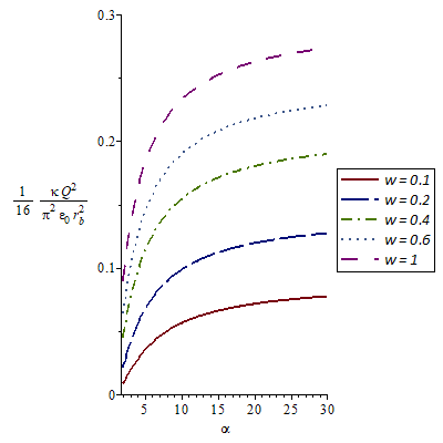
(a) $\frac{\kappa Q^{2}}{16\pi^{2}\epsilon_{0}r_{b}^{2}}$

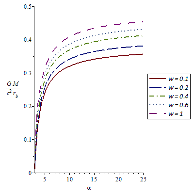
(b) $\frac{GM}{c^{2}r_{b}}$

Figure 5: The dimensionless quantities related with the total electric charge $Q$ (a) and the total mass $M$ (b) as a function of $\alpha$ for some different $\omega$ values and $k=1$.

The non-minimal coupling function (27) becomes explicitly

$$Y(R)=\left[1+\frac{b(3-\omega)(\alpha-2)}{8\omega}\left(\frac{-R}{\alpha b+2b}\right)^{\alpha/(\alpha-2)}\right]^{\frac{3(\omega+1)(\alpha+2)}{\alpha(\omega-3)}}\,.$$ (56)

We also calculate the total charge inside of the sphere with radius $r$ eliminating $b$ from (31)

$$q^{2}(r)=\frac{64\pi^{2}\omega\epsilon_{0}r^{2}}{3\kappa(\omega+1)}\left[1+\frac{br^{\alpha}(3-\omega)(\alpha-2)}{8\omega}\right]^{\frac{4\omega\alpha+6\omega+6}{\alpha(\omega-3)}}\,.$$ (57)

We check that the charge is regular at the origin for $\alpha>2$. Then we can find the the total charge and mass in terms of the boundary radius $r_{b}$, the parameters $\omega$ and $\alpha$ from (43) and (45).

$$Q^{2}=\frac{64\pi^{2}\epsilon_{0}\omega r_{b}^{2}}{3\kappa(\omega+1)}\left[1+\frac{3-\omega}{4\omega}\right]^{\frac{4\omega\alpha+6\omega+6}{\alpha(\omega-3)}},$$ (58)

$$M=\frac{(\alpha-3)}{(\alpha-2)}\frac{c^{2}r_{b}}{3G}+\frac{2c^{2}\omega r_{b}}{3G(\omega+1)}\left[1+\frac{3-\omega}{4\omega}\right]^{\frac{4\omega\alpha+6\omega+6}{\alpha(\omega-3)}}\,.$$ (59)

Variation of the total mass and electric charge as a function of the parameter $\alpha$ is shown in Fig. 5 for some different $\omega$ values. As we can see from the Figures that the increasing $\omega$ values increase the total mass and electric charge. Then we can find upper bound for the total mass and charge by taking $\omega=1$ and $\alpha\rightarrow\infty$.

$$\frac{GM}{c^{2}r_{b}}=0.48,\hskip 56.9055pt\frac{\kappa Q^{2}}{16\pi^{2}\epsilon_{0}r_{b}^{2}}=0.296$$ (60)

In this case, if we observe the gravitational surface redshift of a compact star, we can find $\alpha$ from (46) and $\omega$ from (59) for each observational mass $M$ and boundary radius $r_{b}$ ratio $\frac{M}{r_{b}}$ to describe compact stars with the model. In future, the observations with different redshifts in Table 1 lead to different $\omega$ and $k$ values with the corresponding $\alpha$.

Star	$\frac{M}{r_{b}}\ (\frac{M_{\odot}}{km})$	$\alpha$	$\frac{\kappa^{2}Q^{2}}{16\pi^{2}\epsilon_{0}r_{b}^{2}}$	$z$ (redshift)
EXO 1745-248	$\frac{1.4}{11}$ Ozel2009	3.940	0.054	0.215
4U 1820-30	$\frac{1.58}{9.11}$ Guver2010	5.035	0.067	0.345
4U1608-52	$\frac{1.74}{9.3}$ Guver20102	5.611	0.073	0.390

Table 1: The dimensionless parameter $\alpha$, the dimensionless charge-radius ratio $\frac{\kappa^{2}Q^{2}}{16\pi^{2}\epsilon_{0}r_{b}^{2}}$ and the surface redshift $z$ obtained by using the observational mass $M$ and the radius $r_{b}$ for some neutron stars with $\omega=0.2$ and $k=1$ .

IV Conclusion

We have studied spherically symmetric anisotropic solutions of the non-minimally coupled $Y(R)F^{2}$ theory. We have established the non-minimal model which admits the regular interior metric solutions satisfying conformal symmetry inside the star and Reissner-Nordstrom solution at the exterior assuming the linear equation of state between the radial pressure and energy density as $p_{r}=\omega\rho c^{2}$. We found that the pressures and energy density decrease with the radial distance $r$ inside the star.

We matched the interior and exterior metric, and used the continuity conditions at the boundary of the star. Then we obtained such quantities as total mass, total charge and gravitational surface redshift in terms of the parameters of the model and the boundary radius of the star. We see that the parameter $k$ can not be more than $1$ for non-negative tangential pressure and can not be less than $\frac{2}{\alpha}$ with $\alpha>3$ for the real valued total mass and electric charge. The total mass and electric charge increases with the increasing $\omega$ values, while the gravitational redshift does not change. The total mass-boundary radius ratio has the upper bound $\frac{GM}{c^{2}r_{b}}=0.48$ which is grater than the Buchdahl bound Buchdahl1959 and the bounds given by Mak2001 ; Sert2017 . The gravitational redshift at the surface only depends on the parameter $\alpha$ and increases with increasing $\alpha$ values up to the limit $z=0.732$, which is the same result obtained from the isotropic case with $k=1$ Sert2017 . We also investigated some sub cases such as $\alpha=4,k\neq 1$ and $\alpha>3,k=1$, which can be model of anisotropic stars.

We note that an interesting investigation of anisotropic compact stars was recently given by Salako et al. Salako2018 in the non-conservative theory of gravity. Then, the constants of the interior metric were determined for some known masses and radii. Then the physical parameters such as anisotropy, gravitational redshift, matter density and pressures were calculated and found that this model can describe even super-massive compact stars. On the other hand, in our conservative model (see Sert2017 for energy-momentum conservation), $\alpha$ can be determined by the gravitational surface redshift observations due to (46). Furthermore, if we can also determine the mass-boundary radius ratio $\frac{M}{r_{b}}$ from observations, we can fix one of the two parameters $\omega$ and $k$ via (45). Additionally, the observation of the total charge can fix both of the parameters $\omega$ and $k$ from (43). Thus we can construct a non-minimal $Y(R)F^{2}$ model for each charged compact star. But, the gravitational redshift measurements Cottam2002 ; Lin2010 and total charge predictions do not have enough precise results. However we can predict possible ranges of these quantities.

References

- (1) K. Dev and M. Gleiser Anisotropic Stars II : Stability, Gen.Rel.Grav. 35 1435-1457, 2003, arXiv:gr-qc/0303077.
- (2) R. Ruderman, Pulsars: structure and dynamics, A. Rev. Astr. Astrophys. 10, 427-476, 1972.
- (3) V. Canuto and S. Chitre, Crystallization of dense neutron matter, Phys.Rev. D 9 1587–1613, 1974.
- (4) A. I. Sokolov, Phase transitions in a superfluid neutron liquid, JETP 79, 1137-1140, 1980.
- (5) R.F. Sawyer, Condensed Phase in Neutron-Star Matter, Phys. Rev. Lett. 29, 382-385, 1972.
- (6) R. Kippenhahm and A. Weigert, Stellar structure and evolution, (Springer, Berin, 1990).
- (7) P. Letelier, Anisotropic fluids with two perfect fluid components. Phys. Rev. D 22, 807-813, 1980.
- (8) L. Herrera, N.O. Santos, Local anisotropy in self-gravitating systems. Phys. Rep. 286, 53-130, 1997.
- (9) S.S. Bayin, Anisotropic fluid spheres in general relativity, Phys.Rev. D26 1262, 1982.
- (10) H. O. Silva, C. F. B. Macedo, E. Berti, L. C. B. Crispino, Slowly Rotating Anisotropic Neutron Stars in General Relativity and Scalar-Tensor Theory, 2015, arXiv:1411.6286 [gr-qc].
- (11) M. K. Mak and T. Harko, An Exact Anisotropic Quark Star Model, Chin. J. Astron. Astrophys. Vol. 2, No. 3, 248-259, 2002.
- (12) R.L. Bowers, E.P.T. Liang, Anisotropic spheres in general relativity. Astrophys. J. 188, 657-665, 1974.
- (13) M. K. Mak, T. Harko, Anisotropic Stars in General Relativity, Proc.Roy.Soc.Lond. A459, 393-408, 2003.
- (14) M. S. R. Delgaty, K. Lake, Physical acceptability of isolated, static, spherically symmetric, perfect fluid solutions of Einstein’s equations. Comput. Phys. Commun. 115, 395-415, 1998, arXiv:gr-qc/9809013.
- (15) T. Harko and M.K. Mak, Anisotropic relativistic stellar models, Annalen der Physik, 11, 3-13, 2002, arXiv:gr-qc/0302104.
- (16) M.K. Mak, P.N. Dobson Jr., T. Harko, Exact model for anisotropic relativistic stars, Int. J. Mod. Phys. D 11, 207-221, 2002.
- (17) M. C. Durgapal and R. S. Fuloria, Analytic relativistic model for a superdense star, Gen. Relativ. Gravit. 17 (1985) 671.
- (18) V. Folomeev, Anisotropic neutron stars in gravity, 2018, arXiv:1802.01801 [gr-qc].
- (19) I.G. Salako, A. Jawad, H. Moradpour, Anisotropic compact stars in non-conservative theory of gravity, Int.J.Geom.Meth.Mod.Phys. 15 (2018), 1850093
- (20) R. Stettner, On the stability of homogeneous, spherically symmetric, charged fluids in relativity, Ann. Phys. 80, 212, 1973.
- (21) A. Krasinski, Inhomogeneous cosmological models, (Cambridge University Press , Cambridge, 1997).
- (22) R. Sharma, S. Mukherjee and S.D. Maharaj, General Solution for a Class of Static Charged Spheres. 33, 999, 2001.
- (23) M. K. Mak, and T. Harko, Quark stars admitting a one-parameter group of conformal motions, Int. J. Mod. Phys. D, 13, 149 , 2004, arXiv:gr-qc/0309069.
- (24) M. K. Mak, Peter N. Dobson Jr., T. Harko, Maximum Mass-Radius Ratios for Charged Compact General Relativistic Objects, Europhys.Lett. 55 310-316 , 2001, arXiv:gr-qc/0107011.
- (25) C. G. Böhmer, T. Harko, Bounds on the basic physical parameters for anisotropic compact general relativistic objects, Class.Quant.Grav. 23:22, 6479-6491, 2006, arXiv:gr-qc/0609061.
- (26) K. D. Krori, J. Barua, A singularity-free solution for a charged fluid sphere in general relativity, J. Phys. A: Math. Gen. 8, 508 ,1975.
- (27) G. J. G. Junevicus, An analysis of the Krori-Barua solution, J. Phys. A: Math. Gen. 9, 2069, 1976.
- (28) V. Varela, F. Rahaman, S. Ray, K. Chakraborty, M. Kalam, Charged anisotropic matter with linear or nonlinear equation of state, Phys.Rev.D, 82:044052, 2010, arXiv:1004.2165 [gr-qc].
- (29) F. Rahaman, S. Ray, A. K. Jafry, K. Chacravorty, Singularity-free solutions for anisotropic charged fluids with Chaplygin equation of state, Phys.Rev.D, 82:104055, 2010, arXiv:1007.1889.
- (30) T. Harko, and M.K. Mak, Anisotropic charged fluid spheres in D space-time dimensions, J. Math. Phys. 41, 4752-4764, 2000.
- (31) J. Xu, L.W. Chen, C.M. Ko et al., Isospin and momentum-dependent effective interaction for baryon octet and the properties of hybrid stars. Phys. Rev. C 81, 055803, 2010.
- (32) N.K. Glendenning, S.A. Moszkowski, Reconciliation of neutron-star masses and binding of the in hypernuclei, Phys. Rev. Lett., 67, 2414–2417, 1991.
- (33) P.K. Panda, D.P. Menezes, C. Providencia, Hybrid stars in the quarkmeson coupling model with superconducting quark matter, Phys. Rev. C 69, 025207, 2004.
- (34) D. Page, S. Reddy, Dense matter in compact stars: Theoretical developments and observational constraints, Rev. Nucl. Part. Sci., 56, 327–374, 2006.
- (35) Demorest P B, Pennucci T, Ransom S M, et al. A two-solar-mass neutron star measured using Shapiro delay. Nature, 2010, 467: 1081–1083 arXiv:1010.5788v1 [astro-ph.HE].
- (36) M.H. van Kerkwijk, R. Breton, S.R. Kulkarni, Evidence for a Massive Neutron Star from a Radial-Velocity Study of the Companion to the Black Widow Pulsar PSR B1957+20, Astrophys. J. 728, 95 (2011), arXiv:1009.5427 [astro-ph.HE].
- (37) J.S. Clark et al., Physical parameters of the high-mass X-ray binary 4U1700-37, Astron. Astrophys. 392, 909 (2002).
- (38) P.C. Freire, et al., Eight New Millisecond Pulsars in NGC 6440 and NGC 6441, Astrophys. J. 675, 670 (2008).
- (39) Wen D H, Yan J, Liu X M. One possible mechanism for massive neutron star supported by soft EOS. Int J Mod Phys D, 2012, 21: 1250036
- (40) J. M. Overduin and P. S. Wesson, Dark Matter and Background Light, Physics Reports 402, 267 , 2004, arXiv:astro-ph/0407207.
- (41) H. Baer, K.-Y. Choi, J. E. Kim, and L. Roszkowski, Dark matter production in the early Universe: beyond the thermal WIMP paradigm, Physics Reports 555, 1 , 2015, arXiv:1407.0017
- (42) A. G. Riess et al., Observational Evidence from Supernovae for an Accelerating Universe and a Cosmological Constant, Astron.J.116:1009-1038, 1998, arXiv:astro-ph/9805201.
- (43) S. Perlmutter et al., Measurements of Omega and Lambda from 42 High-Redshift Supernovae, Astrophys.J.517:565-586, 1999, arXiv:astro-ph/9812133.
- (44) R. A. Knop et al., New Constraints on , , and w from an Independent Set of Eleven High-Redshift Supernovae Observed with HST, Astrophys.J.598:102, 2003, arXiv:astro-ph/0309368.
- (45) R. Amanullah et al., Spectra and Light Curves of Six Type Ia Supernovae at and the Union2 Compilation, Astrophys.J. 716:712-738, 2010, arXiv:1004.1711 [astro-ph.CO].
- (46) D. H. Weinberg, M. J. Mortonson, D. J. Eisenstein, C. Hirata, A. G. Riess, and E. Rozo, Observational Probes of Cosmic Acceleration, Physics Reports 530, 87 , 2013, arXiv:1201.2434 [astro-ph.CO].
- (47) D. J. Schwarz, C. J. Copi, D. Huterer and G. D. Starkman, CMB Anomalies after Planck, Class. Quant. Grav. 33 184001 ,2016, arXiv:1510.07929 [astro-ph.CO].
- (48) S. Capozziello and M. De Laurentis, Extended Theories of Gravity, Phys. Rept.509, 167 (2011) arXiv:1108.6266[gr-qc]
- (49) S. Nojiri and S. D. Odintsov, Unified cosmic history in modified gravity: from F(R) theory to Lorentz non-invariant models, Phys. Rept. 505, 59 (2011) arXiv:1011.0544 [gr-qc];
- (50) S. Nojiri and S. D. Odintsov, Introduction to Modified Gravity and Gravitational Alternative for Dark Energy, Int. J. Geom. Meth. Mod. Phys. 4, 115 (2007) arXiv:hep-th/0601213.
- (51) S. Capozziello and V. Faraoni, Beyond Einstein Gravity, Springer, New York (2010).
- (52) S. Capozziello, V. F. Cardone, S. Carloni, A. Troisi, Curvature quintessence matched with observational data, Int. J. Mod. Phys. D 12, 1969 (2003), arXiv:astro-ph/0307018.
- (53) A. Joyce, B. Jain, J. Khoury and M. Trodden, Beyond the Cosmological Standard Model, Physics Reports 568 (2015), pp. 1-98, arXiv:1407.0059 [astro-ph.CO].
- (54) S. Capozziello, M. De Laurentis, The dark matter problem from f(R) gravity viewpoint, Annalen Phys. 524, 545 (2012).
- (55) S. Nojiri, S.D. Odintsov, Modified gravity with negative and positive powers of the curvature: unification of the inflation and of the cosmic acceleration, Phys. Rev. D 68, 123512 (2003)
- (56) S. Nojiri, S.D. Odintsov, Where new gravitational physics comes from: M-theory?, Phys. Lett. B 576, 5 (2003).
- (57) S. Capozziello, M.D. Laurentis, R. Farinelli, and S.D. Odintsov, Mass-radius relation for neutron stars in gravity, Phys.Rev. D93 (2016), 023501, arXiv:1509.04163 [gr-qc].
- (58) A. V. Astashenok, S. Capozziello, and S. D. Odintsov, Maximal neutron star mass and the resolution of the hyperon puzzle in modified gravity, Physical Review D 89, 103509 (2014), arXiv:1401.4546 [gr-qc].
- (59) A.V. Astashenok, S. Capozziello, S.D. Odintsov, Magnetic neutron stars in f( R) gravity, Astrophys Space Sci (2015) 355: 333, arXiv:1405.6663 [gr-qc].
- (60) Z. Jing, D. Wen and X. Zhang, Electrically charged: An effective mechanism for soft EOS supporting massive neutron star, Sci. China Phys. Mech. Astron. 58, no. 10, 109501 (2015).
- (61) A. de la Cruz-Dombriz, A. Dobado, A.L. Maroto, Black holes in theories, Phys. Rev. D 80, 124011 (2009), arXiv:0907.3872 [gr-qc], Phys. Rev. D 83(E), 029903 (2011).
- (62) M. Adak, Ö. Akarsu, T. Dereli, Ö. Sert, Anisotropic inflation with a non-minimally coupled electromagnetic field to gravity, JCAP 11 026 , 2017, arXiv:1611.03393 [gr-qc].
- (63) T. Dereli, Ö. Sert, Non-minimal Couplings of Electromagnetic Fields to Gravity: Static, Spherically Symmetric Solutions, Eur.Phys.J.C71:1589, 2011, arXiv:1102.3863 [gr-qc].
- (64) Ö. Sert, Gravity and Electromagnetism with Y(R)F2-type Coupling and Magnetic Monopole Solutions, Eur. Phys. J. Plus 127: 152 , 2012, arXiv:1203.0898 [gr-qc].
- (65) Ö. Sert, Electromagnetic Duality and New Solutions of the Non-minimally Coupled Y(R)-Maxwell Gravity, Mod. Phys. Lett. A, 2013, arXiv:1303.2436 [gr-qc].
- (66) K. Bamba and S. D. Odintsov, Inflation and late-time cosmic acceleration in non-minimal Maxwell-F(R) gravity and the generation of large-scale magnetic fields, JCAP 0804:024, 2008, arXiv:0801.0954 [astro-ph].
- (67) K. Bamba, S. Nojiri and S. D. Odintsov, Future of the universe in modified gravitational theories: Approaching to the finite-time future singularity, JCAP 0810:045, 2008, arXiv:0807.2575 [hep-th].
- (68) Ö. Sert and M. Adak, An anisotropic cosmological solution to the Maxwell-Y(R) gravity, 2012, arXiv:1203.1531 [gr-qc].
- (69) T. Dereli, Ö. Sert, Non-minimal -Coupled Electromagnetic Fields to Gravity and Static, Spherically Symmetric Solutions, Modern Physics Letters A, Volume 26, Issue 20, pp. 1487-1494, 2011, arXiv:1105.4579 [gr-qc].
- (70) M. S. Turner and L. M. Widrow, Inflation-produced, large-scale magnetic fields, Phys. Rev. D 37, 2743, 1988.
- (71) F. D. Mazzitelli and F. M. Spedalieri, Scalar Electrodynamics and Primordial Magnetic Fields, Phys.Rev. D, 52 6694-6699 , 1995, arXiv:astro-ph/9505140.
- (72) L. Campanelli, P. Cea, G. L. Fogli and L. Tedesco, Inflation-Produced Magnetic Fields in and models, Phys.Rev.D77:123002, 2008, arXiv:0802.2630 [astro-ph].
- (73) A. R. Prasanna, A new invariant for electromagnetic fields in curved space-time, Phys. Lett. 37A, 331 (1971).
- (74) G. W. Horndeski, Conservation of charge and the Einstein–Maxwell field equations, J. Math. Phys. 17, 1980 (1976).
- (75) F. Mueller-Hoissen, and Reinhard Sippel, Spherically symmetric solutions of the non-minimally coupled Einstein-Maxwell equations, Class. Quantum Grav. 5 (1988) 1473-1488.
- (76) F. Mueller-Hoissen, Non-minimal Coupling from Dimensional Reduction of the Gauss-Bonnet action, Physics Letters B, 201, 3, (1988).
- (77) F. Mueller-Hoissen, Modification of Einstein-Yang-Mills theory from dimensional reduction of the Gauss-Bonnet action, Class. Quant. Grav. 5, L35 (1988)
- (78) T. Dereli, G. Üçoluk, Kaluza-Klein reduction of generalised theories of gravity and non-minimal gauge couplings, Class. Q. Grav. 7, 1109 (1990).
- (79) H.A. Buchdahl, On a Lagrangian for non-minimally coupled gravitational and electromagnetic fields, J. Phys. A 12, 1037 (1979)
- (80) I.T. Drummond, S.J. Hathrell, QED vacuum polarization in a background gravitational field and its effect on the velocity of photons, Phys. Rev. D 22, 343 (1980)
- (81) K. E. Kunze, Large scale magnetic fields from gravitationally coupled electrodynamics, Phys. Rev. D 81, 043526 (2010) [arXiv:0911.1101 [astro-ph.CO]].
- (82) Ö. Sert, Regular black hole solutions of the non-minimally coupled Y(R) F2 gravity, J. Math. Phys. 57, 032501 (2016), arXiv:1512.01172 [gr-qc]
- (83) Ö. Sert, Radiation Fluid Stars in the Non-minimally Coupled Y(R)F2 Gravity, Eur. Phys. J. C 77, 97 ,2017.
- (84) Ö. Sert, Compact Stars in the Non-minimally Coupled Electromagnetic Fields to Gravity, Eur. Phys. J. C, 78: 241, 2018, arXiv:1801.07493 [gr-qc].
- (85) L. Herrera, J. Ponce de Leon, Isotropic and charged spheres admitting a one‐parameter group of conformal motions,J. Math. Phys. 26, 2302 ,1985.
- (86) L. Herrera, J. Ponce de Leon, Anisotropic spheres admitting a one‐parameter group of conformal motions, J. Math. Phys. 26, 2018, 1985.
- (87) L. Herrera, J. Ponce de Leon, Perfect fluid spheres admitting a one‐parameter group of conformal motions,J. Math. Phys. 26, 778, 1985.
- (88) J. Cottam, F. Paerels, M. Mendez, Gravitationally redshifted absorption lines in the X-ray burst spectra of a neutron star, Nature 2002, 420, 51–54, arXiv:astro-ph/0211126
- (89) J. Lin, F. Ozel, D. Chakrabarty, D. Psaltis, The Incompatibility of Rapid Rotation with Narrow Photospheric X-ray Lines in EXO 0748-676, Astrophys. J. 723, 1053–1056, 2010 arXiv:1007.1451 [astro-ph.HE].
- (90) F. Özel, T. Guver, and D. Psaltis, The Mass and Radius of the Neutron Star in EXO 1745-248, APJ 693:1775–1779, 2009, arXiv:0810.1521 [astro-ph].
- (91) T. Guver, P. Wroblewski, L. Camarota, F. Özel, The Mass and Radius of the Neutron Star in 4U 1820-30, APJ , 719, 1807, 2010, arXiv:1002.3825 [astro-ph.HE].
- (92) T. Guver, F. Özel, A. Cabrera-Lavers, and P. Wroblewski, The Distance, Mass, and Radius of the Neutron Star in 4U 1608-52, Astrophys.J.712:964-973, 2010, arXiv:0811.3979 [astro-ph].
- (93) H.A. Buchdahl, General Relativistic Fluid Spheres, Phys. Rev., 116 1027 (1959).