A Lyapunov-based Approach to Safe Reinforcement Learning

Abstract

In many real-world reinforcement learning (RL) problems, besides optimizing the main objective function, an agent must concurrently avoid violating a number of constraints. In particular, besides optimizing performance it is crucial to guarantee the safety of an agent during training as well as deployment (e.g. a robot should avoid taking actions - exploratory or not - which irrevocably harm its hardware). To incorporate safety in RL, we derive algorithms under the framework of constrained Markov decision problems (CMDPs), an extension of the standard Markov decision problems (MDPs) augmented with constraints on expected cumulative costs. Our approach hinges on a novel Lyapunov method. We define and present a method for constructing Lyapunov functions, which provide an effective way to guarantee the global safety of a behavior policy during training via a set of local, linear constraints. Leveraging these theoretical underpinnings, we show how to use the Lyapunov approach to systematically transform dynamic programming (DP) and RL algorithms into their safe counterparts. To illustrate their effectiveness, we evaluate these algorithms in several CMDP planning and decision-making tasks on a safety benchmark domain. Our results show that our proposed method significantly outperforms existing baselines in balancing constraint satisfaction and performance.

1 Introduction

Reinforcement learning (RL) has shown exceptional successes in a variety of domains such as video games [24] and recommender systems [37], where the main goal is to optimize a single return. However, in many real-world problems, besides optimizing the main objective (the return), there can exist several conflicting constraints that make RL challenging. In particular, besides optimizing performance it is crucial to guarantee the safety of an agent in deployment [5] as well as during training [2]. For example, a robot agent should avoid taking actions which irrevocably harm its hardware; a recommender system must avoid presenting harmful or offending items to users.

Sequential decision-making in non-deterministic environments has been extensively studied in the literature under the framework of Markov decision problems (MDPs). To incorporate safety into the RL process, we are particularly interested in deriving algorithms under the context of constrained Markov decision problems (CMDPs), which is an extension of MDPs with expected cumulative constraint costs. The additional constraint component of CMDPs increases flexibility in modeling problems with trajectory-based constraints, when compared with other approaches that customize immediate costs in MDPs to handle constraints [31]. As shown in numerous applications from robot motion planning [29, 25, 10], resource allocation [23, 17], and financial engineering [1, 38], it is more natural to define safety over the whole trajectory, instead of over particular state and action pairs. Under this framework, we denote an agent’s behavior policy to be safe if it satisfies the cumulative cost constraints of the CMDP.

Despite the capabilities of CMDPs, they have not been very popular in RL. One main reason is that, although optimal policies of finite CMDPs are Markov and stationary, and with known models the CMDP can be solved using linear programming (LP) [3], it is unclear how to extend this algorithm to handle cases when the model is unknown, or when the state and action spaces are large or continuous. A well-known approach to solve CMDPs is the Lagrangian method [4, 14], which augments the standard expected reward objective with a penalty on constraint violation. With a fixed Lagrange multiplier, one can use standard dynamic programming (DP) or RL algorithms to solve for an optimal policy. With a learnable Lagrange multiplier, one must solve the resulting saddle point problem. However, several studies [20] showed that iteratively solving the saddle point is apt to run into numerical stability issues. More importantly, the Lagrangian policy is only safe asymptotically and makes little guarantee with regards to safety of the behavior policy during each training iteration.

Motivated by these observations, several recent works have derived surrogate algorithms for solving CMDPs, which transform the original constraint to a more conservative one that yields an easier problem to solve. A straight-forward approach is to replace the cumulative constraint cost with a conservative stepwise surrogate constraint [9] that only depends on current state and action pair. Since this surrogate constraint can be easily embedded into the admissible control set, this formulation can be modeled by an MDP that has a restricted set of admissible actions. Another surrogate algorithm was proposed by [13], in which the algorithm first computes a uniform super-martingale constraint value function surrogate w.r.t. all policies. Then one computes a CMDP feasible policy by optimizing the surrogate problem using the lexicographical ordering method [36]. These methods are advantageous in the sense that (i) there are RL algorithms available to handle the surrogate problems (for example see [12] for the step-wise surrogate, and see [26] for the super-martingale surrogate), (ii) the policy returned by this method is safe, even during training. However, the main drawback of these approaches is their conservativeness. Characterizing sub-optimality performance of the corresponding solution policy also remains a challenging task. On the other hand, recently in policy gradient, [2] proposed the constrained policy optimization (CPO) method that extends trust-region policy optimization (TRPO) to handle the CMDP constraints. While this algorithm is scalable, and its policy is safe during training, analyzing its convergence is challenging, and applying this methodology to other RL algorithms is non-trivial.

Lyapunov functions have been extensively used in control theory to analyze the stability of dynamic systems [19, 27]. A Lyapunov function is a type of scalar potential function that keeps track of the energy that a system continually dissipates. Besides modeling physical energy, Lyapunov functions can also represent abstract quantities, such as the steady-state performance of a Markov process [15]. In many fields, Lyapunov functions provide a powerful paradigm to translate global properties of a system to local ones, and vice-versa. Using Lyapunov functions in RL was first studied by [30], where Lyapunov functions were used to guarantee closed-loop stability of an agent. Recently [6] used Lyapunov functions to guarantee a model-based RL agent’s ability to re-enter an “attraction region” during exploration. However no previous works have used Lyapunov approaches to explicitly model constraints in a CMDP. Furthermore, one major drawback of these approaches is that the Lyapunov functions are hand-crafted, and there are no principled guidelines on designing Lyapunov functions that can guarantee an agent’s performance.

The contribution of this paper is four-fold. First we formulate the problem of safe reinforcement learning as a CMDP and propose a novel Lyapunov approach for solving them. While the main challenge of other Lyapunov-based methods is to design a Lyapunov function candidate, we propose an LP-based algorithm to construct Lyapunov functions w.r.t. generic CMDP constraints. We also show that our method is guaranteed to always return a feasible policy and, under certain technical assumptions, it achieves optimality. Second, leveraging the theoretical underpinnings of the Lyapunov approach, we present two safe DP algorithms – safe policy iteration (SPI) and safe value iteration (SVI) – and analyze the feasibility and performance of these algorithms. Third, to handle unknown environment models and large state/action spaces, we develop two scalable, safe RL algorithms – (i) safe DQN, an off-policy fitted $Q-$iteration method, and (ii) safe DPI, an approximate policy iteration method. Fourth, to illustrate the effectiveness of these algorithms, we evaluate them in several tasks on a benchmark 2D planning problem, and show that they outperform common baselines in terms of balancing performance and constraint satisfaction.

2 Preliminaries

We consider the RL problem in which the agent’s interaction with the system is modeled as a Markov decision process (MDP). A MDP is a tuple $(\mathcal{X},\mathcal{A},c,P,x_{0})$, where $\mathcal{X}=\mathcal{X}^{\prime}\cup\{x_{\text{Term}}\}$ is the state space, with transient state space $\mathcal{X}^{\prime}$ and terminal state $x_{\text{Term}}$; $\mathcal{A}$ is the action space; $c(x,a)\in[0,C_{\max}]$ is the immediate cost function (negative reward); $P(\cdot|x,a)$ is the transition probability distribution; and $x_{0}\in\mathcal{X}^{\prime}$ is the initial state. Our results easily generalize to random initial states and random costs, but for simplicity we will focus on the case of deterministic initial state and immediate cost. In a more general setting where cumulative constraints are taken into account, we define a constrained Markov decision process (CMDP), which extends the MDP model by introducing additional costs and associated constraints. A CMDP is defined by $(\mathcal{X},\mathcal{A},c,d,P,x_{0},d_{0})$, where the components $\mathcal{X},\mathcal{A},c,P,x_{0}$ are the same for the unconstrained MDP; $d(x)\in[0,D_{\max}]$ is the immediate constraint cost; and $d_{0}\in\mathbb{R}_{\geq 0}$ is an upper bound for the expected cumulative (through time) constraint cost. To formalize the optimization problem associated with CMDPs, let $\Delta$ be the set of Markov stationary policies, i.e., $\Delta(x)=\{\pi(\cdot|x)\mathrel{\mathop{\mathchar 58\relax}}\mathcal{X}\rightarrow\mathbb{R}_{\geq 0s}\mathrel{\mathop{\mathchar 58\relax}}\sum_{a}\pi(a|x)=1\}$ for any state $x\in\mathcal{X}$. Also let $\mathrm{T}^{*}$ be a random variable corresponding to the first-hitting time of the terminal state $x_{\text{Term}}$ induced by policy $\pi$. In this paper, we follow the standard notion of transient MDPs and assume that the first-hitting time is uniformly bounded by an upper bound $\overline{\mathrm{T}}$. This assumption can be justified by the fact that sample trajectories collected in most RL algorithms consist of a finite stopping time (also known as a time-out); the assumption may also be relaxed in cases where a discount $\gamma<1$ is applied on future costs. For notational convenience, at each state $x\in\mathcal{X}^{\prime}$, we define the generic Bellman operator w.r.t. policy $\pi\in\Delta$ and generic cost function $h$: $T_{\pi,h}[V](x)=\sum_{a}\pi(a|x)\!\left[h(x,a)\!+\!\sum_{x^{\prime}\in\mathcal{X}^{\prime}}\!\!P(x^{\prime}|x,a)V(x^{\prime})\right].$

Given a policy $\pi\in\Delta$, an initial state $x_{0}$, the cost function is defined as $\mathcal{C}_{\pi}(x_{0})\mathrel{\mathop{\mathchar 58\relax}}=\mathbb{E}\big{[}\sum_{t=0}^{\mathrm{T}^{*}-1}c(x_{t},a_{t})\mid x_{0},\pi\big{]},$ and the safety constraint is defined as $\mathcal{D}_{\pi}(x_{0})\leq d_{0}$ where the safety constraint function is given by $\mathcal{D}_{\pi}(x_{0})\mathrel{\mathop{\mathchar 58\relax}}=\mathbb{E}\big{[}\sum_{t=0}^{\mathrm{T}^{*}-1}d(x_{t})\mid x_{0},\pi\big{]}.$ In general the CMDP problem we wish to solve is given as follows:

Problem $\mathcal{OPT}$: Given an initial state $x_{0}$ and a threshold $d_{0}$, solve $\min_{\pi\in\Delta}\,\left\{\mathcal{C}_{\pi}(x_{0})\mathrel{\mathop{\mathchar 58\relax}}\mathcal{D}_{\pi}(x_{0})\leq d_{0}\right\}.$ If there is a non-empty solution, the optimal policy is denoted by $\pi^{*}$.

Under the transient CMDP assumption, Theorem 8.1 in [3], shows that if the feasibility set is non-empty, then there exists an optimal policy in the class of stationary Markovian policies $\Delta$. To motivate the CMDP formulation studied in this paper, in Appendix A, we include two real-life examples in modeling safety using (i) the reachability constraint, and (ii) the constraint that limits the agent’s visits to undesirable states. Recently there has been a number of works on CMDP algorithms; their details can be found in Appendix B.

3 A Lyapunov Approach for Solving CMDPs

In this section we develop a novel methodology for solving CMDPs using the Lyapunov approach. To start with, without loss of generality assume we have access to a baseline feasible policy of problem $\mathcal{OPT}$, namely $\pi_{B}\in\Delta$. We define a non-empty set of Lyapunov functions w.r.t. initial state $x_{0}\in\mathcal{X}$ and constraint threshold $d_{0}$ as

$$\mathcal{L}_{\pi_{B}}(x_{0},d_{0})\!=\!\bigg{\{}\!L\!\mathrel{\mathop{\mathchar 58\relax}}\mathcal{X}\!\rightarrow\!\mathbb{R}_{\geq 0}\!\mathrel{\mathop{\mathchar 58\relax}}\!T_{\pi_{B},d}[L](x)\!\leq\!L(x),\forall x\in\mathcal{X}^{\prime};\,L(x)=0,\,\forall x\in\mathcal{X}\setminus\mathcal{X}^{\prime};\,L(x_{0})\leq d_{0}\bigg{\}}.$$ (1)

For any arbitrary Lyapunov function $L\in\mathcal{L}_{\pi_{B}}(x_{0},d_{0})$, denote by $\mathcal{F}_{L}(x)=\left\{\pi(\cdot|x)\in\Delta\mathrel{\mathop{\mathchar 58\relax}}T_{\pi,d}[L](x)\leq\!L(x)\right\}$ the set of $L-$induced Markov stationary policies. Since $T_{\pi,d}$ is a contraction mapping [7], clearly any $L-$induced policy $\pi$ has the following property: $\mathcal{D}_{\pi}(x)=\lim_{k\rightarrow\infty}T^{k}_{\pi,d}[L](x)\leq L(x)$, $\forall x\in\mathcal{X}^{\prime}$. Together with the property of $L(x_{0})\leq d_{0}$, this further implies any $L-$induced policy is a feasible policy of problem $\mathcal{OPT}$. However in general the set $\mathcal{F}_{L}(x)$ does not necessarily contain any optimal policies of problem $\mathcal{OPT}$, and our main contribution is to design a Lyapunov function (w.r.t. a baseline policy) that provides this guarantee. In other words, our main goal is to construct a Lyapunov function $L\in\mathcal{L}_{\pi_{B}}(x_{0},d_{0})$ such that

$$L(x)\geq T_{\pi^{*},d}[L](x),\,\,L(x_{0})\leq d_{0}.$$ (2)

Before getting into the main results, we consider the following important technical lemma, which states that with appropriate cost-shaping, one can always transform the constraint value function $\mathcal{D}_{\pi^{*}}(x)$ w.r.t. optimal policy $\pi^{*}$ into a Lyapunov function that is induced by $\pi_{B}$, i.e., $L_{\epsilon}(x)\in\mathcal{L}_{\pi_{B}}(x_{0},d_{0})$. The proof of this lemma can be found in Appendix C.1.

Lemma 1.

There exists an auxiliary constraint cost $\epsilon\mathrel{\mathop{\mathchar 58\relax}}\mathcal{X}^{\prime}\rightarrow\mathbb{R}$ such that the Lyapunov function is given by $L_{\epsilon}(x)=\mathbb{E}\left[\sum_{t=0}^{\mathrm{T}^{*}-1}d(x_{t})+\epsilon(x_{t})\mid\pi_{B},x\right],\forall x\in\mathcal{X}^{\prime},$ and $L_{\epsilon}(x)=0$ for $x\in\mathcal{X}\setminus\mathcal{X}^{\prime}$. Moreover, $L_{\epsilon}$ is equal to the constraint value function w.r.t. $\pi^{*}$, i.e., $L_{\epsilon}(x)=\mathcal{D}_{\pi^{*}}(x)$.

From the structure of $L_{\epsilon}$, one can see that the auxiliary constraint cost function $\epsilon$ is uniformly bounded by $\epsilon^{*}(x)\mathrel{\mathop{\mathchar 58\relax}}=2\overline{\mathrm{T}}D_{\max}D_{TV}(\pi^{*}||\pi_{B})(x)$, i.e., $\epsilon(x)\in[-\epsilon^{*}(x),\epsilon^{*}(x)]$, for any $x\in\mathcal{X}^{\prime}$. However in general it is unclear how to construct such a cost-shaping term $\epsilon$ without explicitly knowing $\pi^{*}$ a-priori. Rather, inspired by this result, we consider the bound $\epsilon^{*}$ to propose a Lyapunov function candidate $L_{\epsilon^{*}}$. Immediately from its definition, this function has the following properties:

$$L_{\epsilon^{*}}(x)\geq T_{\pi_{B},d}[L_{\epsilon^{*}}](x),\,\,L_{\epsilon^{*}}(x)\geq\max\left\{\mathcal{D}_{\pi^{*}}(x),\mathcal{D}_{\pi_{B}}(x)\right\}\geq 0,\,\forall x\in\mathcal{X}^{\prime}.$$ (3)

The first property is due to the facts that: (i) $\epsilon^{*}$ is a non-negative cost function; (ii) $T_{\pi_{B},d+\epsilon^{*}}$ is a contraction mapping, which by the fixed point theorem [7] implies $L_{\epsilon^{*}}(x)=T_{\pi_{B},d+\epsilon^{*}}[L_{\epsilon^{*}}](x)\geq T_{\pi_{B},d}[L_{\epsilon^{*}}](x),\,\forall x\in\mathcal{X}^{\prime}.$ For the second property, from the above inequality one concludes that the Lyapunov function $L_{\epsilon^{*}}$ is a uniform upper bound to the constraint cost, i.e., $L_{\epsilon^{*}}(x)\geq\mathcal{D}_{\pi_{B}}(x)$, because the constraint cost $\mathcal{D}_{\pi_{B}}(x)$ w.r.t. policy $\pi_{B}$ is the unique solution to the fixed-point equation $T_{\pi_{B},d}[V](x)=V(x)$, $x\in\mathcal{X}^{\prime}$. On the other hand, by construction $\epsilon^{*}(x)$ is an upper-bound of the cost-shaping term $\epsilon(x)$. Therefore Lemma 1 implies that Lyapunov function $L_{\epsilon^{*}}$ is a uniform upper bound to the constraint cost w.r.t. optimal policy $\pi^{*}$, i.e., $L_{\epsilon^{*}}(x)\geq\mathcal{D}_{\pi^{*}}(x)$.

To show that $L_{\epsilon^{*}}$ is a Lyapunov function that satisfies (2), we propose the following condition that enforces a baseline policy $\pi_{B}$ to be sufficiently close to an optimal policy $\pi^{*}$.

Assumption 1.

The feasible baseline policy $\pi_{B}$ satisfies the following condition: $\max_{x\in\mathcal{X}^{\prime}}\epsilon^{*}(x)\!\leq\!D_{\max}\cdot\min\left\{\frac{d_{0}-\mathcal{D}_{\pi_{B}}(x_{0})}{\overline{\mathrm{T}}D_{\max}},\frac{\overline{\mathrm{T}}D_{\max}-\overline{\mathcal{D}}}{\overline{\mathrm{T}}D_{\max}+\overline{\mathcal{D}}}\right\},$ where $\overline{\mathcal{D}}=\max_{x\in\mathcal{X}^{\prime}}\max_{\pi}\mathcal{D}_{\pi}(x)$.

This condition characterizes the maximum allowable distance between $\pi_{B}$ and $\pi^{*}$, such that the set of $L_{\epsilon^{*}}-$induced policies contains an optimal policy. To formalize this claim, we have the following main result showing that $L_{\epsilon^{*}}\in\mathcal{L}_{\pi_{B}}(x_{0},d_{0})$, and the set of policies $\mathcal{F}_{L_{\epsilon^{*}}}$ contains an optimal policy.

Theorem 1.

Suppose the baseline policy $\pi_{B}$ satisfies Assumption $1$, then on top of the properties in (3), the Lyapunov function candidate $L_{\epsilon^{*}}$ also satisfies the properties in (2), and therefore its induced feasible set of policies $\mathcal{F}_{L_{\epsilon^{*}}}$ contains an optimal policy.

The proof of this theorem is given in Appendix C.2. Suppose the distance between the baseline policy and the optimal policy can be estimated effectively. Using the above result, one can immediately determine if the set of $L_{\epsilon^{*}}-$induced policies contain an optimal policy. Equipped with the set of $L_{\epsilon^{*}}-$induced feasible policies, consider the following safe Bellman operator:

$$T[V](x)=\left\{\begin{array}[]{cl}\min_{\pi\in\mathcal{F}_{L_{\epsilon^{*}}}(x)}T_{\pi,c}[V](x)&\text{if $x\in\mathcal{X}^{\prime}$}\\ 0&\text{otherwise}\end{array}\right..$$ (4)

Using standard analysis of Bellman operators, one can show that $T$ is a monotonic and contraction operator (see Appendix C.3 for proof). This further implies that the solution of the fixed point equation $T[V](x)=V(x)$, $\forall x\in\mathcal{X}$, is unique. Let $V^{*}$ be such a value function. The following theorem shows that under Assumption 1, $V^{*}(x_{0})$ is a solution to problem $\mathcal{OPT}$.

Theorem 2.

Suppose the baseline policy $\pi_{B}$ satisfies Assumption 1. Then, the fixed-point solution at $x=x_{0}$, i.e., $V^{*}(x_{0})$, is equal to the solution of problem $\mathcal{OPT}$. Furthermore, an optimal policy can be constructed by $\pi^{*}(\cdot|x)\!\in\!\arg\min_{\pi\in\mathcal{F}_{L_{\epsilon^{*}}}(x)}T_{\pi,c}[V^{*}](x)$, $\forall x\!\in\!\mathcal{X}^{\prime}$.

The proof of this theorem can be found in Appendix C.4. This shows that under Assumption 1 an optimal policy of problem $\mathcal{OPT}$ can be solved using standard DP algorithms. Notice that verifying whether $\pi_{B}$ satisfies this assumption is still challenging because one requires a good estimate of $D_{TV}(\pi^{*}||\pi_{B})$. Yet to the best of our knowledge, this is the first result that connects the optimality of CMDP to Bellman’s principle of optimality. Another key observation is that, in practice we will explore ways of approximating $\epsilon^{*}$ via bootstrapping, and empirically show that this approach achieves good performance while guaranteeing safety at each iteration. In particular, in the next section we will illustrate how to systematically construct a Lyapunov function using an LP in the planning scenario, and using function approximation in RL for guaranteeing safety during learning.

4 Safe Reinforcement Learning Using Lyapunov Functions

Motivated by the challenge of computing a Lyapunov function $L_{\epsilon^{*}}$ such that its induced set of policies contains $\pi^{*}$, in this section we approximate $\epsilon^{*}$ with an auxiliary constraint cost $\widetilde{\epsilon}$, which is the largest auxiliary cost that satisfies the Lyapunov condition: $L_{\widetilde{\epsilon}}(x)\geq T_{\pi_{B},d}[L_{\widetilde{\epsilon}}](x),\,\,\forall x\in\mathcal{X}^{\prime}$ and the safety condition $L_{\widetilde{\epsilon}}(x_{0})\leq d_{0}$. The larger the $\widetilde{\epsilon}$, the larger the set of policies $\mathcal{F}_{L_{\widetilde{\epsilon}}}$. Thus by choosing the largest such auxiliary cost, we hope to have a better chance of including the optimal policy $\pi^{*}$ in the set of feasible policies. So, we consider the following LP problem:

$$\widetilde{\epsilon}\in\!\arg\!\max_{\epsilon\mathrel{\mathop{\mathchar 58\relax}}\mathcal{X}^{\prime}\rightarrow\mathbb{R}_{\geq 0}}\!\!\Bigg{\{}\!\sum_{x\in\mathcal{X}^{\prime}}\epsilon(x)\!\mathrel{\mathop{\mathchar 58\relax}}d_{0}-\mathcal{D}_{\pi_{B}}(x_{0})\geq\mathbf{1}(x_{0})^{\top}(I-\{P(x^{\prime}|x,\pi_{B})\}_{x,x^{\prime}\in\mathcal{X}^{\prime}})^{-1}\epsilon\!\Bigg{\}}.$$ (5)

Here $\mathbf{1}(x_{0})$ represents a one-hot vector in which the non-zero element is located at $x=x_{0}$.

On the other hand, whenever $\pi_{B}$ is a feasible policy, then the problem in (5) always has a non-empty solution. Furthermore, notice that $\mathbf{1}(x_{0})^{\top}(I-\{P(x^{\prime}|x,\pi_{B})\}_{x,x^{\prime}\in\mathcal{X}^{\prime}})^{-1}\mathbf{1}(x)$ represents the total visiting probability $\mathbb{E}[\sum_{t=0}^{\mathrm{T}^{*}-1}\mathbf{1}\{x_{t}=x\}\mid x_{0},\pi_{B}]$ from initial state $x_{0}$ to any state $x\in\mathcal{X}^{\prime}$, which is a non-negative quantity. Therefore, using the extreme point argument in LP [22], one can simply conclude that the maximizer of problem (5) is an indicator function whose non-zero element locates at state $\underline{x}$ that corresponds to the minimum total visiting probability from $x_{0}$, i.e., $\widetilde{\epsilon}(x)={(d_{0}-\mathcal{D}_{\pi_{B}}(x_{0}))\cdot\mathbf{1}\{x=\underline{x}\}}/{\mathbb{E}[\sum_{t=0}^{\mathrm{T}^{*}-1}\mathbf{1}\{x_{t}=\underline{x}\}\mid x_{0},\pi_{B}]}\geq 0,\,\forall x\in\mathcal{X}^{\prime}$, where $\underline{x}\in\arg\min_{x\in\mathcal{X}^{\prime}}\mathbb{E}[\sum_{t=0}^{\mathrm{T}^{*}-1}\mathbf{1}\{x_{t}=x\}\mid x_{0},\pi_{B}]$. On the other hand, suppose we further restrict the structure of $\widetilde{\epsilon}(x)$ to be a constant function, i.e., $\widetilde{\epsilon}(x)=\widetilde{\epsilon}$, $\forall x\in\mathcal{X}^{\prime}$. Then one can show that the maximizer is given by $\widetilde{\epsilon}(x)={(d_{0}-\mathcal{D}_{\pi_{B}}(x_{0}))}/{\mathbb{E}[\mathrm{T}^{*}\mid x_{0},\pi_{B}]}$, $\forall x\in\mathcal{X}^{\prime}$, where $\mathbf{1}(x_{0})^{\top}(I-\{P(x^{\prime}|x,\pi_{B})\}_{x,x^{\prime}\in\mathcal{X}^{\prime}})^{-1}[1,\ldots,1]^{\top}=\mathbb{E}[\mathrm{T}^{*}\mid x_{0},\pi_{B}]$ is the expected stopping time of the transient MDP. In cases when computing the expected stopping time is expensive, then one reasonable approximation is to replace the denominator of $\widetilde{\epsilon}$ with the upper-bound $\overline{\mathrm{T}}$.

Using this Lyapunov function $L_{\widetilde{\epsilon}}$, we propose the safe policy iteration (SPI) in Algorithm 1, in which the Lyapunov function is updated via bootstrapping, i.e., at each iteration $L_{\widetilde{\epsilon}}$ is re-computed using (5), w.r.t. the current baseline policy. Properties of SPI are summarized in the following proposition.

  Input: Initial feasible policy $\pi_{0}$;

  for $k=0,1,2,\ldots$ do

     Step 0: With $\pi_{b}=\pi_{k}$, evaluate the Lyapunov function $L_{\epsilon_{k}}$, where $\epsilon_{k}$ is a solution of (5)

     Step 1: Evaluate the cost value function $V_{\pi_{k}}(x)=\mathcal{C}_{\pi_{k}}(x)$; Then update the policy by solving the following problem: $\pi_{k+1}(\cdot|x)\in\arg\!\min_{\pi\in\mathcal{F}_{L_{\epsilon_{k}}}(x)}T_{\pi,c}[V_{\pi_{k}}](x),\forall x\in\mathcal{X}^{\prime}$

  end for

  Return Final policy $\pi_{k^{*}}$

Algorithm 1 Safe Policy Iteration (SPI)

Proposition 1.

Algorithm 1 has following properties: (i) Consistent Feasibility, i.e., suppose the current policy $\pi_{k}$ is feasible, then the updated policy $\pi_{k+1}$ is also feasible, i.e., $\mathcal{D}_{\pi_{k}}(x_{0})\leq d_{0}$ implies $\mathcal{D}_{\pi_{k+1}}(x_{0})\leq d_{0}$; (ii) Monotonic Policy Improvement, i.e., the cumulative cost induced by $\pi_{k+1}$ is lower than or equal to that by $\pi_{k}$, i.e., $\mathcal{C}_{\pi_{k+1}}(x)\leq\mathcal{C}_{\pi_{k}}(x)$ for any $x\in\mathcal{X}^{\prime}$; (iii) Convergence, i.e., suppose a strictly concave regularizer is added to optimization problem (5) and a strictly convex regularizer is added to policy optimization step. Then the policy sequence asymptotically converges.

The proof of this proposition is given in Appendix C.5, and the sub-optimality performance bound of SPI can be found in Appendix C.6. Analogous to SPI, we also propose a safe value iteration (SVI), in which the Lyapunov function estimate is updated at every iteration via bootstrapping, using the current optimal value estimate. Details of SVI is given in Algorithm 2, and its properties are summarized in the following proposition (whose proof is given in Appendix C.7).

  Input: Initial $Q-$function $Q_{0}$; Initial Lyapunov function $L_{\epsilon_{0}}$ w.r.t. auxiliary cost function $\epsilon_{0}(x)\!=\!0$;

  for $k=0,1,2,\ldots$ do

     Step 0: Compute $Q-$function $Q_{k+1}(x,a)=c(x,a)+\sum_{x^{\prime}}\!P(x^{\prime}|x,a)\min_{\pi\in\mathcal{F}_{L_{\epsilon_{k}}}(x^{\prime})}\pi(\cdot|x^{\prime})^{\top}Q_{k}(x^{\prime},\cdot)$ and policy $\pi_{k}(\cdot|x)\in\arg\min_{\pi\in\mathcal{F}_{L_{\epsilon_{k}}}(x)}\pi(\cdot|x)^{\top}Q_{k}(x,\cdot)$

     Step 1: With $\pi_{B}=\pi_{k}$, construct the Lyapunov function $L_{\epsilon_{k+1}}$, where $\epsilon_{k+1}$ is a solution of (5);

  end for

  Return Final policy $\pi_{k^{*}}$

Algorithm 2 Safe Value Iteration (SVI)

Proposition 2.

Algorithm 2 has following properties: (i) Consistent Feasibility; (ii) Convergence.

To justify the notion of bootstrapping, in both SVI and SPI, the Lyapunov function is updated based on the best baseline policy (the policy that is feasible and by far has the lowest cumulative cost). Once the current baseline policy $\pi_{k}$ is sufficiently close to an optimal policy $\pi^{*}$, then by Theorem 1 one concludes that the $L_{\widetilde{\epsilon}}-$induced set of policies contains an optimal policy. Although these algorithms do not have optimality guarantees, empirically they often return a near-optimal policy.

In each iteration, the policy optimization step in SPI and SVI requires solving $|\mathcal{X}^{\prime}|$ LP sub-problems, where each of them has $|\mathcal{A}|+2$ constraints and has a $|\mathcal{A}|-$dimensional decision-variable. Collectively, at each iteration its complexity is $O(|\mathcal{X}^{\prime}||\mathcal{A}|^{2}(|\mathcal{A}|+2))$. While in the worst case SVI converges in $K=O(\overline{\mathrm{T}})$ steps [7], and SPI converges in $K=O(|\mathcal{X}^{\prime}||\mathcal{A}|\overline{\mathrm{T}}\log\overline{\mathrm{T}})$ steps [35], in practice $K$ is much smaller than $|\mathcal{X}^{\prime}||\mathcal{A}|$. Therefore, even with the additional complexity of policy evaluation in SPI that is $O(\overline{\mathrm{T}}|\mathcal{X}^{\prime}|^{2})$, or the complexity of updating $Q-$function in SVI that is $O(|\mathcal{A}|^{2}|\mathcal{X}^{\prime}|^{2})$, the complexity of these methods is $O(K|\mathcal{X}^{\prime}||\mathcal{A}|^{3}+K|\mathcal{X}^{\prime}|^{2}|\mathcal{A}|^{2})$, which in practice is much lower than that of the dual LP method, whose complexity is $O(|\mathcal{X}^{\prime}|^{3}|\mathcal{A}|^{3})$ (see Section B for details).

4.1 Lyapunov-based Safe RL Algorithms

In order to improve scalability of SVI and SPI, we develop two off-policy safe RL algorithms, namely safe DQN and safe DPI, which replace the value and policy updates in safe DP with function approximations. Their pseudo-codes can be found in Appendix D. Before going into their details, we first introduce the policy distillation method, which will be later used in the safe RL algorithms.

Policy Distillation:

Consider the following LP problem for policy optimization in SVI and SPI:

$$\pi^{\prime}(\cdot|x)\in\arg\min_{\pi\in\Delta}\left\{\pi(\cdot|x)^{\top}Q(x,\cdot)\mathrel{\mathop{\mathchar 58\relax}}(\pi(\cdot|x)-\pi_{B}(\cdot|x))^{\top}Q_{L}(x,\cdot)\leq\widetilde{\epsilon}^{\prime}(x)\right\},$$ (6)

where $Q_{L}(x,a)=d(x)+\widetilde{\epsilon}^{\prime}(x)+\sum_{x^{\prime}}P(x^{\prime}|x,a)L_{\widetilde{\epsilon}^{\prime}}(x^{\prime})$ is the state-action Lyapunov function. When the state-space is large (or continuous), explicitly solving for a policy becomes impossible without function approximation. Consider a parameterized policy $\pi_{\phi}$ with weights $\phi$. Utilizing the distillation concept [33], after computing the optimal action probabilities w.r.t. a batch of states, the policy $\pi_{\phi}$ is updated by solving $\phi^{*}\in\arg\min_{\phi}\frac{1}{m}\sum_{m=1}^{M}\sum_{t=0}^{\overline{\mathrm{T}}-1}D_{\text{JSD}}(\pi_{\phi}(\cdot|x_{t,m})\parallel\pi^{\prime}(\cdot|x_{t,m}))$, where the Jensen-Shannon divergence. The pseudo-code of distillation is given in Algorithm 3.

Safe $Q-$learning (SDQN):

Here we sample an off-policy mini-batch of state-action-costs-next-state samples from the replay buffer and use it to update the value function estimates that minimize the MSE losses of Bellman residuals. Specifically, we first construct the state-action Lyapunov function estimate $\widehat{Q}_{L}(x,a;\theta_{D},\theta_{T})=\widehat{Q}_{D}(x,a;\theta_{D})+\widetilde{\epsilon}^{\prime}\cdot\widehat{Q}_{T}(x,a;\theta_{T})$, by learning the constraint value network $\widehat{Q}_{D}$ and stopping time value network $\widehat{Q}_{T}$ respectively. With a current baseline policy $\pi_{k}$, one can use function approximation to approximate the auxiliary constraint cost (which is the solution of (5),) by $\widetilde{\epsilon}^{\prime}(x)=\widetilde{\epsilon}^{\prime}={(d_{0}-\pi_{k}(\cdot|x_{0})^{\top}\widehat{Q}_{D}(x_{0},\cdot;\theta_{D}))}/{\pi_{k}(\cdot|x_{0})^{\top}\widehat{Q}_{T}(x_{0},\cdot;\theta_{T})}$. Equipped with the Lyapunov function, in each iteration one can do a standard DQN update, except that the optimal action probabilities are computed via solving (6). Details of SDQN is given in Algorithm 4.

Safe Policy Improvement (SDPI):

Similar to SDQN, in this algorithm we first sample an off-policy mini-batch of samples from the replay buffer and use it to update the value function estimates (w.r.t. objective, constraint, and stopping-time estimate) that minimize MSE losses. Different from SDQN, in SDPI the value estimation is done using policy evaluation, which means that the objective $Q-$function is trained to minimize the Bellman residual w.r.t. actions generated by the current policy $\pi_{k}$, instead of the greedy actions. Using the same construction as in SDQN for auxiliary cost $\widetilde{\epsilon}^{\prime}$, and state-action Lyapunov function $\widehat{Q}_{L}$, we then perform a policy improvement step by computing a set of greedy action probabilities from (6), and constructing an updated policy $\pi_{k+1}$ using policy distillation. Assuming the function approximations (for both value and policy) have low errors, SDPI resembles several interesting properties from SPI, such as maintaining safety during training and improving policy monotonically. To improve learning stability, instead of the full policy update one can further consider a partial update $\pi_{k+1}=(1-\alpha)\pi_{k}+\alpha\pi^{\prime}$, where $\alpha\in(0,1)$ is a mixing constant that controls safety and exploration [2, 18]. Details of SDPI is summarized in Algorithm 5.

In terms of practical implementations, in Appendix E we include techniques to improve stability during training, to handle continuous action space, and to scale up policy optimization step in (6).

5 Experiments

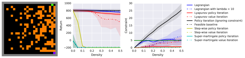
Figure 1: Results of various planning algorithms on the grid-world environment with obstacles, with x-axis showing the obstacle density. From the leftmost column, the first figure illustrates the 2D planning domain example ($\rho=0.25$). The second and the third figure show the average return and the average cumulative constraint cost of the CMDP methods respectively. The fourth figure displays all the methods used in the experiment. The shaded regions indicate the $80\%$ confidence intervals. Clearly the safe DP algorithms compute policies that are safe and have good performance.

Motivated by the safety issues of RL in [21], we validate our safe RL algorithms using a stochastic 2D grid-world motion planning problem. In this domain, an agent (e.g., a robotic vehicle) starts in a safe region and its objective is to travel to a given destination. At each time step the agent can move to any of its four neighboring states. Due to sensing and control noise, however, with probability $\delta$ a move to a random neighboring state occurs. To account for fuel usage, the stage-wise cost of each move until reaching the destination is $1$, while the reward achieved for reaching the destination is $1000$. Thus, we would like the agent to reach the destination in the shortest possible number of moves. In between the starting point and the destination there is a number of obstacles that the agent may pass through but should avoid for safety; each time the agent is on an obstacle it incurs a constraint cost of $1$. Thus, in the CMDP setting, the agent’s goal is to reach the destination in the shortest possible number of moves while passing through obstacles at most $d_{0}$ times or less. For demonstration purposes, we choose a $25\times 25$ grid-world (see Figure 1) with a total of $625$ states. We also have a density ratio $\rho\in(0,1)$ that sets the obstacle-to-terrain ratio. When $\rho$ is close to $0$, the problem is obstacle-free, and if $\rho$ is close to $1$, then the problem becomes more challenging. In the normal problem setting, we choose a density $\rho=0.3$, an error probability $\delta=0.05$, a constraint threshold $d_{0}=5$, and a maximum horizon of $200$ steps. The initial state is located in $(24,24)$, and the goal is placed in $(0,\alpha)$, where $\alpha\in[0,24]$ is a uniform random variable. To account for statistical significance, the results of each experiment are averaged over $20$ trials.

CMDP Planning: In this task we have explicit knowledge on reward function and transition probability. The main goal is to compare our safe DP algorithms (SPI and SVI) with the following common CMDP baseline methods: (i) Step-wise Surrogate, (ii) Super-martingale Surrogate, (iii) Lagrangian, and (iv) Dual LP. Since the methods in (i) and (ii) are surrogate algorithms, we will also evaluate these methods with both value iteration and policy iteration. To illustrate the level of sub-optimality, we will also compare the returns and constraint costs of these methods with baselines that are generated by maximizing return or minimizing constraint cost of two separate MDPs. The main objective here is to illustrate that safe DP algorithms are less conservative than other surrogate methods, are more numerically stable than the Lagrangian method, and are more computationally efficient than the Dual LP method (see Appendix F), without using function approximations.

Figure 1 presents the results on returns and the cumulative constraint costs of the aforementioned CMDP methods over a spectrum of $\rho$ values, ranging from $0$ to $0.5$. In each method, the initial policy is a conservative baseline policy $\pi_{B}$ that minimizes the constraint cost. Clearly from the empirical results, although the polices generated by the four surrogate algorithms are feasible, they do not have significant policy improvements, i.e., return values are close to that of the initial baseline policy. Over all density settings, the SPI algorithm consistently computes a solution that is feasible and has good performance. The solution policy returned by SVI is always feasible, and it has near-optimal performance when the obstacle density is low. However, due to numerical instability its performance degrades as $\rho$ grows. Similarly, the Lagrangian methods return a near-optimal solution over most settings, but due to numerical issues their solutions start to violate constraint as $\rho$ grows.

Safe Reinforcement Learning: In this section we present the results of RL algorithms on this safety task. We evaluate their learning performance on two variants: one in which the observation is a one-hot encoding the of the agent’s location, and the other in which the observation is the 2D image representation of the grid map. In each of these, we evaluate performance when $d_{0}=1$ and $d_{0}=5$. We compare our proposed safe RL algorithms, SDPI and SDQN, to their unconstrained counterparts, DPI and DQN, as well as the Lagrangian approach to safe RL, in which the Lagrange multiplier is optimized via extensive grid search. Details of the experimental setup is given in Appendix F. To make the tasks more challenging, we initialize the RL algorithms with a randomized baseline policy.

Figure 2 shows the results of these methods across all task variants. Clearly, we see that SDPI and SDQN can adequately solve the tasks and compute agents with good return performance (similar to that of DQN and DPI in some cases), while guaranteeing safety. Another interesting observation in the SDQN and SDPI algorithms is that, once the algorithm finds a safe policy, then all updated policies remain safe during throughout training. On the contrary, the Lagrangian approaches often achieve worse rewards and are more apt to violate the constraints during training , and the performance is very sensitive to initial conditions. Furthermore, in some cases (in experiment with $d_{0}=5$ and with discrete observation) the Lagrangian method cannot guarantee safety throughout training.

	Discrete obs, $d_{0}=5$	Discrete obs, $d_{0}=1$	Image obs, $d_{0}=5$	Image obs, $d_{0}=1$
Constraints                    Rewards

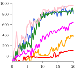
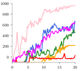
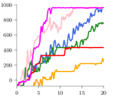
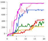
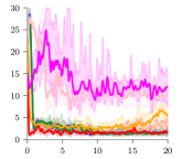
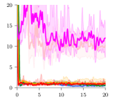
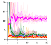
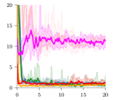
Figure 2: Results of various RL algorithms on the grid-world environment with obstacles, with x-axis in thousands of episodes. We include runs using discrete observations (a one-hot encoding of the agent’s position) and image observations (showing the entire RGB 2D map of the world). We discover that the Lyapunov-based approaches can perform safe learning, despite the fact that the environment dynamics model is not known and that deep function approximations are necessary.

6 Conclusion

In this paper we formulated the problem of safe RL as a CMDP and proposed a novel Lyapunov approach to solve CMDPs. We also derived an effective LP-based method to generate Lyapunov functions, such that the corresponding algorithm guarantees feasibility, and optimality under certain conditions. Leveraging these theoretical underpinnings, we showed how Lyapunov approaches can be used to transform DP (and RL) algorithms into their safe counterparts, that only requires straightforward modifications in the algorithm implementations. Empirically we validated our theoretical findings in using Lyapunov approach to guarantee safety and robust learning in RL. In general, our work represents a step forward in deploying RL to real-world problems in which guaranteeing safety is of paramount importance. Future research will focus on two directions. On the algorithmic perspective, one major extension is to apply Lyapunov approach to policy gradient algorithms, and compare its performance with CPO in continuous RL problems. On the practical perspective, future work includes evaluating the Lyapunov-based RL algorithms on several real-world testbeds.

Appendix A Safety Constraints in Planning Problems

To motivate the CMDP formulation studied in this paper, in this section we include two real-life examples of modeling safety using the reachability constraint, and the constraint that limits the agent’s visits to undesirable states.

A.1 Reachability Constraint

Reachability is a common concept in motion-planning and engineering applications, where for any given policy $\pi$ and initial state $x_{0}$, the following the constraint function is considered:

$$\mathbb{P}(\exists t\in\{0,1,\ldots,\mathrm{T}^{*}-1\},x_{t}\in\mathcal{S}_{H}\mid x_{0},\pi).$$

Here $\mathcal{S}_{H}$ represents the real subset of hazardous regions for the states and actions. Therefore, the constraint cost represents the probability of reaching an unsafe region at any time before the state reaches the terminal state. To further analyze this constraint function, one notices that

$$\begin{split}\mathbb{P}(\exists t\in\{0,1,\ldots,\mathrm{T}^{*}-1\},x_{t}\in\mathcal{S}_{H}\mid x_{0},\pi)=&\mathbb{P}\left(\bigcup_{t=0}^{\mathrm{T}^{*}-1}\bigcap_{j=0}^{t-1}\{x_{j}\not\in\mathcal{S}_{H}\}\cap\{x_{t}\in\mathcal{S}_{H}\}\mid x_{0},\pi\right)\\ =&\mathbb{E}\left[\sum_{t=0}^{\mathrm{T}^{*}-1}\prod_{j=0}^{t-1}\mathbf{1}\{x_{j}\not\in\mathcal{S}_{H}\}\cdot\mathbf{1}\{x_{t}\in\mathcal{S}_{H}\}\mid x_{0},\pi\right].\end{split}$$

In this case, a policy $\pi$ is deemed safe if the reachability probability to the unsafe region is bounded by threshold $d_{0}\in(0,1)$, i.e.,

$$\mathbb{P}(\exists t\in\{0,1,\ldots,\mathrm{T}^{*}-1\},x_{t}\in\mathcal{S}_{H}\mid x_{0},\pi)\leq d_{0}.$$ (7)

To transform the reachability constraint into a standard CMDP constraint, we define an additional state $s\in\{0,1\}$ that keeps track of the reachability status at time $t$. Here $s_{t}=1$ indicates the system has never visited a hazardous region up till time $t$, and otherwise $s_{t}=0$. Let $s_{0}=1$, we can easily see that by defining the following deterministic transition

$$s_{t}=s_{t-1}\cdot\mathbf{1}\{x_{t}\not\in\mathcal{S}_{H}\},\,\,\forall t\geq 1,$$

$s_{t}$ has the following formulation: $s_{t}=\prod_{j=0}^{t-1}\mathbf{1}\{x_{j}\not\in\mathcal{S}_{H}\}.$

Collectively, with the state augmentation $\hat{x}=(x,s)$, one defines the augmented CMDP $(\hat{\mathcal{X}},\mathcal{A},C,\hat{D},\hat{P},\hat{x}_{0},d_{0})$, where $\hat{\mathcal{X}}=\mathcal{X}\times\{0,1\}$ is the augmented state space, $\hat{d}(\hat{x})=s\cdot d(x)$ is the augmented constraint cost, $\hat{P}(\hat{x}^{\prime}|\hat{x},a)=P(x^{\prime}|x,a)\cdot\mathbf{1}\{s^{\prime}=s\cdot\mathbf{1}\{x\not\in\mathcal{S}_{H}\}\}$ is the augmented transition probability, and $\hat{x_{0}}=(x_{0},1)$ is the initial (augmented) state. By using this augmented CMDP, immediately the reachability constraint is equivalent to $\mathbb{E}\big{[}\sum_{t=0}^{\mathrm{T}^{*}-1}\hat{d}(\hat{x}_{t})\mid x_{0},\pi\big{]}\leq d_{0}.$

A.2 Constraint w.r.t. Undesirable Regions of States

Consider the notion of safety where one restricts the total visiting frequency of an agent to an undesirable region (of states). This notion of safety appears in applications such as system maintenance, in which the system can only tolerate its state to visit (in expectation) a hazardous region, namely $\mathcal{S}_{H}$, for a fixed number of times. Specifically, for given initial state $x_{0}$, consider the following constraint that bounds the total frequency of visiting $\mathcal{S}_{H}$ with a pre-defined threshold $d_{0}$, i.e., $\mathbb{E}\big{[}\sum_{t=0}^{\mathrm{T}^{*}-1}d(x_{t})\mid x_{0},\pi\big{]}\leq d_{0},$ where $d(x_{t})=\mathbf{1}\{x_{t}\in\mathcal{S}_{H}\}$. To model this notion of safety using a CMDP, one can rewrite the above constraint using the constraint immediate cost $d(x)=\mathbf{1}\{x\in\mathcal{S}_{H}\}$, and the constraint threshold $d_{0}$. To study the connection between the reachability constraint, and the above constraint w.r.t. undesirable region, notice that

$$\mathbb{E}\left[\sum_{t=0}^{\mathrm{T}^{*}-1}\prod_{j=0}^{t-1}\mathbf{1}\{x_{j}\not\in\mathcal{S}_{H}\}\cdot\mathbf{1}\{x_{t}\in\mathcal{S}_{H}\}\mid x_{0},\pi\right]\leq\mathbb{E}\left[\sum_{t=0}^{\mathrm{T}^{*}-1}\mathbf{1}\{x_{t}\in\mathcal{S}_{H}\}\mid x_{0},\pi\right].$$

This clearly indicates that any policies which satisfies the constraint w.r.t. undesirable region, also satisfies the reachability constraint.

Appendix B Existing Approaches for Solving CMDPs

Before going to the main result, we first revisit several existing CMDP algorithms in the literature, which later serve as the baselines for comparing with our safe CMDP algorithms. For the sake of brevity, we will only provide an overview of these approaches here and defer their details to Appendix B.1.

The Lagrangian Based Algorithm:

The standard way of solving problem $\mathcal{OPT}$ is by applying the Lagrangian method. To start with, consider the following minimax problem: $\min_{\pi\in\Delta}\max_{\lambda\geq 0}\,\,\mathcal{C}_{\pi}(x_{0})+\lambda(\mathcal{D}_{\pi}(x_{0})-d_{0}),$ where $\lambda$ is the Lagrange multiplier w.r.t. the CMDP constraint. According to Theorem 9.9 and Theorem 9.10 in [3], the optimal policy $\pi^{*}$ of problem $\mathcal{OPT}$ can be calculated by solving the following Lagrangian function $\pi^{*}\in\arg\min_{\pi\in\Delta}\mathcal{C}_{\pi}(x_{0})+\lambda^{*}_{d_{0}}\mathcal{D}_{\pi}(x_{0}),$ where $\lambda^{*}_{d_{0}}$ is the optimal Lagrange multiplier. Utilizing this result, one can compute the saddle point pair $(\pi^{*},\lambda^{*})$ using primal-dual iteration. Specifically, for a given $\lambda\geq 0$, solve the policy minimization problem using standard dynamic programming with $\lambda-$parametrized Bellman operator $T_{\lambda}[V](x)=\min_{\pi\in\Delta(x)}T_{\pi,c+\lambda d}[V](x)$ if $x\in\mathcal{X}$; For a given policy $\pi$, solve for the following linear optimization problem: $\max_{\lambda\geq 0}\,\,\mathcal{C}_{\pi}(x_{0})+\lambda(\mathcal{D}_{\pi}(x_{0})-d_{0})$. Based on Theorem 9.10 in [3], this procedure will asymptotically converge to the saddle point solution. However, this algorithm presents several major challenges. (i) In general there is no known convergence rate guarantees, several studies [20] also showed that using primal-dual first-order iterative method to find saddle point may run into numerical instability issues; (ii) Choosing a good initial estimate of the Lagrange multiplier is not intuitive; (iii) Following the same arguments from [2], during iteration the policy may be infeasible w.r.t. problem $\mathcal{OPT}$, and feasibility is guaranteed after the algorithm converges. This is hazardous in RL when one needs to execute the intermediate policy (which may be unsafe) during training.

The Dual LP Based Algorithm:

Another method of solving problem $\mathcal{OPT}$ is based on computing its occupation measures w.r.t. the optimal policy. In transient MDPs, for any given policy $\pi$ and initial state $x_{0}$, the state-action occupation measure is $\rho_{\pi}(x,a)=\mathbb{E}\left[\sum_{t=0}^{\mathrm{T}^{*}-1}\mathbf{1}\{x_{t}=x,a_{t}=a\}\mid x_{0},\pi\right]$, which characterizes the total visiting probability of state-action pair $(x,a)\in\mathcal{X}\times\mathcal{A}$, induced by policy $\pi$ and initial state $x_{0}$. Utilizing this quantity, Theorem 9.13 in [3], has shown that problem $\mathcal{OPT}$ can be reformulated as a linear programming (LP) problem (see Equation (8) to (9) in Appendix B.1), whose decision variable is of dimension $|\mathcal{X}^{\prime}||\mathcal{A}|$, and it has $2|\mathcal{X}^{\prime}||\mathcal{A}|+1$ constraints. Let $\rho^{*}$ be the solution of this LP, the optimal Markov stationary policy is given by $\pi^{*}(a|x)={\rho^{*}(x,a)}/{\sum_{a\in\mathcal{A}}\rho^{*}(x,a)}$. To solve this problem, one can apply the standard algorithm such as interior point method, which is a strong polynomial time algorithm with complexity $O(|\mathcal{X}^{\prime}|^{2}|\mathcal{A}|^{2}(2|\mathcal{X}^{\prime}||\mathcal{A}|+1))$ [8]. While this is a straight-forward methodology, it can only handle CMDPs with finite state and action spaces. Furthermore, this approach is computationally expensive when the size of these spaces are large. To the best of our knowledge, it is also unclear how to extend this approach to RL, when transition probability and immediate reward/constraint reward functions are unknown.

Step-wise Constraint Surrogate Approach:

This approach transforms the multi-stage CMDP constraint into a sequence of step-wise constraints, where each step-wise constraint can be directly embedded into set of admissible actions in the Bellman operator. To start with, for any state $x\in\mathcal{X}^{\prime}$, consider the following feasible set of policies: $\mathcal{F}^{\text{SW}}(d_{0},x)=\big{\{}\pi\in\Delta\mathrel{\mathop{\mathchar 58\relax}}\sum_{a\in\mathcal{A}}\sum_{x^{\prime}\in\mathcal{X}^{\prime}}\pi(a|x)P(x^{\prime}|x,a)d(x^{\prime})\leq\frac{d_{0}}{\overline{\mathrm{T}}}\big{\}},$ where $\overline{\mathrm{T}}$ is the upper-bound of the MDP stopping time. Based on (10) in Appendix B.1, one deduces that every policy $\pi$ in $\bigcap_{x\in\mathcal{X}^{\prime}}\mathcal{F}^{\text{SW}}(d_{0},x)$ is a feasible policy w.r.t. problem $\mathcal{OPT}$. Motivated by this observation, a solution policy can be solved by $\min_{\pi\in\bigcap_{x\in\mathcal{X}^{\prime}}\mathcal{F}^{\text{SW}}(d_{0},x)}\,\mathbb{E}\left[\sum_{t=0}^{\mathrm{T}^{*}-1}c(x_{t},a_{t})\mid x_{0},\pi\right]$. One benefit of studying this surrogate problem is that its solution satisfies the Bellman optimality condition w.r.t. the step-wise Bellman operator as $T^{\text{SW}}[V](x)=\min_{\pi\in\mathcal{F}^{\text{SW}}(d_{0},x)}\sum_{a}\pi(a|x)\big{[}c(x,a)+\sum_{x^{\prime}\in\mathcal{X}^{\prime}}P(x^{\prime}|x,a)V(x^{\prime})\big{]}$ for any $x\in\mathcal{X}^{\prime}$. In particular $T^{\text{SW}}$ is a contraction operator, which implies that there exists a unique solution $V^{*,\text{SW}}$ to fixed point equation $T^{\text{SW}}[V](x)=V(x)$ for $x\in\mathcal{X}^{\prime}$ such that $V^{*,\text{SW}}(x_{0})$ is a solution to the surrogate problem. Therefore this problem can be solved by standard DP methods such as value iteration or policy iteration. Furthermore, based on the structure of $\mathcal{F}^{\text{SW}}(d_{0},x)$, any surrogate policy is feasible w.r.t. problem $\mathcal{OPT}$. However, the major drawback is that the step-wise constraint in $\mathcal{F}^{\text{SW}}(d_{0},x)$ can be much more stringent than the original safety constraint in problem $\mathcal{OPT}$.

Super-martingale Constraint Surrogate Approach:

This surrogate algorithm is originally proposed by [13], where the CMDP constraint is reformulated as the surrogate value function $\mathcal{DS}_{\pi}(x)=\max\left\{d_{0},\mathcal{D}_{\pi}(x)\right\}$ at initial state $x\in\mathcal{X}^{\prime}$. It has been shown that an arbitrary policy $\pi$ is a feasible policy of the CMDP if and only if $\mathcal{DS}_{\pi}(x_{0})=d_{0}$. Notice that $\mathcal{DS}_{\pi}$ is known as a super-martingale surrogate, due to the inequality $\mathcal{DS}_{\pi}(x)\leq T^{DS}_{\pi}[\mathcal{DS}_{\pi}](x)$ with respect to the contraction Bellman operator $T^{DS}_{\pi}[V](x)=\sum_{a\in\mathcal{A}}\pi(a|x)\max\left\{d_{0},d(x)+\sum_{x^{\prime}\in\mathcal{X}^{\prime}}P(x^{\prime}|x,a)V(x^{\prime})\right\}$ of the constraint value function. However, for arbitrary policy $\pi$, in general it is non-trivial to compute the value function $\mathcal{DS}_{\pi}(x)$, and instead one can easily compute its upper-bound value function $\overline{\mathcal{DS}}_{\pi}(x)$ which is the solution of the fixed-point equation $V(x)=T^{DS}_{\pi}[V](x),\,\,\,\forall x\in\mathcal{X}^{\prime}$, using standard dynamic programming techniques. To better understand how this surrogate value function guarantees feasibility in problem $\mathcal{OPT}$, at each state $x\in\mathcal{X}^{\prime}$ consider the optimal value function of the minimization problem $\overline{\mathcal{DS}}(x)=\min_{\pi\in\Delta}\overline{\mathcal{DS}}_{\pi}(x)$. Then whenever $\overline{\mathcal{DS}}(x_{0})\leq d_{0}$, the corresponding solution policy $\pi$ is a feasible policy of problem $\mathcal{OPT}$, i.e., $\mathcal{D}_{\pi}(x_{0})\leq\overline{\mathcal{DS}}_{\pi}(x_{0})=d_{0}$. Now define $\mathcal{F}^{\text{DS}}(x)\mathrel{\mathop{\mathchar 58\relax}}=\!\big{\{}\pi\in\Delta\mathrel{\mathop{\mathchar 58\relax}}T^{DS}_{\pi}[\overline{\mathcal{DS}}](x)=\!\overline{\mathcal{DS}}(x)\!\big{\}}$ as the set of refined feasible policies induced by $\overline{\mathcal{DS}}$. If the condition $\overline{\mathcal{DS}}(x_{0})\leq d_{0}$ holds, then all the policies in $\mathcal{F}^{\text{DS}}(x)$ are feasible w.r.t. problem $\mathcal{OPT}$. Utilizing this observation, a surrogate solution policy of problem $\mathcal{OPT}$ can be found by computing the solution policy of the fixed-point equation $T_{\mathcal{F}^{\text{DS}}}[V](x)=V(x)$, for $x\in\mathcal{X}^{\prime}$, where $T_{\mathcal{F}^{\text{DS}}}[V](x)=\min_{\pi\in\mathcal{F}^{\text{DS}}(d_{0},x)}T_{\pi,c}[V](x)$. Notice that $T_{\mathcal{F}^{\text{DS}}}$ is a contraction operator, this procedure can also be solved using standard DP methods. The major benefit of this 2-step approach is that the computation of the feasibility set is decoupled from solving the optimization problem. This allows us to apply approaches such as the lexicographical ordering method from multi-objective stochastic optimal control methods [32] to solve the CMDP, for which the constraint value function has a higher lexicographical order than the objective value function. However, since the refined set of feasible policies is constructed prior to policy optimization, it might still be overly conservative. Furthermore, even if there exists a non-trivial solution policy to the surrogate problem, characterizing its sub-optimality performance bound remains a challenging task.

B.1 Details of Existing Solution Algorithms

In this section, we provide the details of the existing algorithms for solving CMDPs.

The Lagrangian Based Algorithm:

The standard way of solving problem $\mathcal{OPT}$ is by applying the Lagrangian method. To start with, consider the following minimax problem:

$$\min_{\pi\in\Delta}\max_{\lambda\geq 0}\,\,\mathcal{C}_{\pi}(x_{0})+\lambda(\mathcal{D}_{\pi}(x_{0})-d_{0}),$$

where $\lambda$ is the Lagrange multiplier of the CMDP constraint, and the Lagrangian function is given by

$$\mathcal{L}_{x_{0},d_{0}}(\pi,\lambda)=\mathcal{C}_{\pi}(x_{0})+\lambda(\mathcal{D}_{\pi}(x_{0})-d_{0})=\mathbb{E}\left[\sum_{t=0}^{\mathrm{T}^{*}-1}c(x_{t},a_{t})+\lambda d(x_{t})\mid\pi,x_{0}\right]-\lambda d_{0}.$$

A solution pair $(\pi^{*},\lambda^{*})$ is considered as a saddle point of Lagrangian function $\mathcal{L}_{x_{0},d_{0}}(\pi,\lambda)$ if the following condition holds:

$$\mathcal{L}_{x_{0},d_{0}}(\pi^{*},\lambda)\leq L_{x_{0},d_{0}}(\pi,\lambda)\leq\mathcal{L}_{x_{0},d_{0}}(\pi,\lambda^{*}),\,\,\forall\pi,\lambda\geq 0.$$

According to Theorem 9.10 in [3], suppose the interior set of feasible set of problem $\mathcal{OPT}$ is non-empty, then there exists a solution pair $(\pi^{*},\lambda^{*})$ to the minimax problem that is a saddle point of Lagrangian function $\mathcal{L}_{x_{0},d_{0}}(\pi,\lambda)$. Furthermore, Theorem 9.9 in [3] shows that strong duality holds:

$$\min_{\pi\in\Delta}\max_{\lambda\geq 0}\,\,\mathcal{L}_{x_{0},d_{0}}(\pi,\lambda)=\max_{\lambda\geq 0}\min_{\pi\in\Delta}\,\,\mathcal{L}_{x_{0},d_{0}}(\pi,\lambda).$$

This implies that the optimal policy $\pi^{*}\in\Delta$ can be calculated by solving the following Lagrangian function $\pi^{*}\in\arg\min_{\pi\in\Delta}\mathcal{L}_{x_{0},d_{0}}(\pi,\lambda^{*}),$ with optimal Lagrange multiplier $\lambda^{*}$.

Utilizing the structure of the Lagrangian function $\mathcal{L}_{x_{0},d_{0}}(\pi,\lambda)$, for any fixed Lagrange multiplier $\lambda\geq 0$, consider the $\lambda-$Bellman operator $T_{\lambda}[V]$, where

$$T_{\lambda}[V](x)=\left\{\begin{array}[]{cl}\min_{\pi\in\Delta(x)}\,T_{\pi,c+\lambda d}[V](x)&\text{if $x\in\mathcal{X}^{\prime}$,}\\ 0&\text{otherwise}.\end{array}\right.$$

Since $T_{\lambda}[V]$ is a $\gamma-$contraction operator, by the Bellman principle of optimality, there is a unique solution $V^{*}$ to the fixed point equation $T_{\lambda}[V](x)=V(x)$ for $x\in\mathcal{X}$, which can be solved by dynamic programming algorithms, such as value iteration or policy iteration. Furthermore, the $\lambda-$optimal policy $\pi^{*}_{\lambda}$ has the form of

$$\pi^{*}_{\lambda}(\cdot|x)\in\arg\min_{\pi\in\Delta(x)}T_{\pi,c+\lambda d}[V^{*}](x)\quad\text{if $x\in\mathcal{X}^{\prime}$, }$$

and $\pi^{*}_{\lambda}(\cdot|x)$ is an arbitrary probability distribution function if $x\not\in\mathcal{X}^{\prime}$.

The Dual LP Based Algorithm:

The other commonly-used method for solving problem $\mathcal{OPT}$ is based on computing its occupation measures w.r.t. the optimal policy. In a transient MDP, for any given policy $\pi$ and initial state $x_{0}\in\mathcal{X}^{\prime}$ the state-action occupation measure is defined as

$$\rho_{\pi,x_{0}}(x,a)=\mathbb{E}\left[\sum_{t=0}^{\mathrm{T}^{*}-1}\mathbf{1}\{x_{t}=x,a_{t}=a\}\mid x_{0},\pi\right],\,\,\forall x\in\mathcal{X},\,\,\forall a\in\mathcal{A},$$

and the occupation measure at state $x\in\mathcal{X}$ is defined as $\rho_{\pi,x_{0}}(x)=\sum_{a\in\mathcal{A}}\rho_{\pi,x_{0}}(x,a)$. Clearly these two occupation measures are related by the following property: $\rho_{\pi,x_{0}}(x,a)=\rho_{\pi,x_{0}}(x)\cdot\pi(a|x)$. Furthermore, using the fact that a occupation measure $\rho_{\pi,x_{0}}(x,a)$ is indeed the sum of visiting distribution of the transient MDP induced by policy $\pi$, one clearly sees that it satisfies the following set of constraints:

$$\begin{split}\mathcal{Q}(x_{0})\!=\!\bigg{\{}\!\rho\mathrel{\mathop{\mathchar 58\relax}}\mathcal{X}^{\prime}\times\mathcal{A}\rightarrow\mathbb{R}\mathrel{\mathop{\mathchar 58\relax}}&\rho(x,a)\geq 0,\forall x\in\mathcal{X}^{\prime},a\in\mathcal{A},\\ &\!\!\!\sum_{x_{p}\in\mathcal{X}^{\prime},a\in\mathcal{A}}\!\!\rho(x_{p},a)(\mathbf{1}\{x_{p}=x\}\!-\!P(x|x_{p},a))\!=\!\mathbf{1}\{x=x_{0}\}\bigg{\}}.\end{split}$$

Therefore, by Theorem 9.13 in [3], equivalently problem $\mathcal{OPT}$ can be solved by the LP optimization problem with $2|\mathcal{X}^{\prime}||\mathcal{A}|+1$ constraints:

$$\min_{\rho\in\mathcal{Q}(x_{0})} \mathcal{\sum}_{x\in\mathcal{X}^{\prime},a\in\mathcal{A}}\rho(x,a)c(x,a)$$ (8)

subject to $$\sum_{x\in\mathcal{X}^{\prime},a\in\mathcal{A}}\rho(x,a)d(x)\leq d_{0},$$ (9)

and equipped with the minimizer minimizer $\rho^{*}\in\mathcal{Q}(x_{0})$, the (non-uniform) optimal Markovian stationary policy is given by the following form:

$$\pi^{*}(a|x)=\frac{\rho^{*}(x,a)}{\sum_{a\in\mathcal{A}}\rho^{*}(x,a)},\,\,\forall x\in\mathcal{X}^{\prime},\,\,\forall a\in\mathcal{A}.$$

Step-wise Constraint Surrogate Approach:

To start with, without loss of generality assume that the agent is safe at the initial phase, i.e., $d(x_{0})\leq 0$. For any state $x\in\mathcal{X}^{\prime}$, consider the following feasible set of policies:

$$\mathcal{F}^{\text{SW}}(d_{0},x)=\left\{\pi\in\Delta(x)\mathrel{\mathop{\mathchar 58\relax}}\sum_{a\in\mathcal{A}}\sum_{x^{\prime}\in\mathcal{X}^{\prime}}\pi(a|x)P(x^{\prime}|x,a)d(x^{\prime})\leq\frac{d_{0}}{\overline{\mathrm{T}}}\right\},$$

where $\overline{\mathrm{T}}$ is the uniform upper-bound of the random stopping time in the transient MDP. Immediately, for any policy $\pi\in\bigcap_{x\in\mathcal{X}^{\prime}}\mathcal{F}^{\text{SW}}(d_{0},x)$, one has the following inequality:

$$\begin{split}\mathbb{E}\left[\sum_{t=0}^{\mathrm{T}^{*}-1}d(x_{t})\mid\pi,x_{0}\right]=&d(x_{0})+\sum_{x\in\mathcal{X}^{\prime},a\in\mathcal{A}}\rho_{\pi,x_{0}}(x,a)\sum_{x^{\prime}\in\mathcal{X}^{\prime}}P(x^{\prime}|x,a)d(x^{\prime})\\ \leq&\mathbb{E}\left[\sum_{t=0}^{\mathrm{T}^{*}-1}\frac{d_{0}}{\overline{\mathrm{T}}}\mid\pi,x_{0}\right]\leq d_{0},\end{split}$$ (10)

where $\rho_{\pi,x_{0}}(x,a)=\mathbb{E}\left[\sum_{t=0}^{\mathrm{T}^{*}-1}\mathbf{1}\{x_{t}=x\}|\pi,x_{0}\right]$ is the state-action occupation measure with initial state $x_{0}$ and policy $\pi$, which implies that the policy $\pi$ is safe, i.e., $\mathcal{D}_{\pi}(x_{0})\leq d_{0}$. Equipped with this property, we propose the following surrogate problem for problem $\mathcal{OPT}$, whose solution (if exists) is guaranteed to be safe:

Problem $\mathcal{OPT}^{\text{SW}}$: Given an initial state $x_{0}$, a threshold $d_{0}$, solve $\min_{\pi\in\bigcap_{x\in\mathcal{X}^{\prime}}\mathcal{F}^{\text{SW}}(d_{0},x)}\,\mathbb{E}\left[\sum_{t=0}^{\mathrm{T}^{*}-1}c(x_{t},a_{t})\mid x_{0},\pi\right].$

To solve problem $\mathcal{OPT}^{\text{SW}}$, for each state $x\in\mathcal{X}^{\prime}$ define the step-wise Bellman operator as

$$T^{\text{SW}}[V](x)=\min_{\pi\in\mathcal{F}^{\text{SW}}(d_{0},x)}T_{\pi,c}[V](x).$$

Based on the standard arguments in [7], the Bellman operator $T^{\text{SW}}$ is a contraction operator, which implies that there exists a unique solution $V^{*,\text{SW}}$ to the fixed-point equation $T^{\text{SW}}[V](x)=V(x)$, for any $x\in\mathcal{X}^{\prime}$, such that $V^{*,\text{SW}}(x_{0})$ is a solution to problem $\mathcal{OPT}^{\text{SW}}$.

Super-martingale Constraint Surrogate Approach:

The following surrogate algorithm is proposed by [13]. Before going to the main algorithm, first consider the following surrogate constraint value function w.r.t. policy $\pi\in\Delta$ and state $x\in\mathcal{X}^{\prime}$:

$$\begin{split}\mathcal{DS}_{\pi}(x)=&\max\left\{d_{0},\mathcal{D}_{\pi}(x)\right\}=\max\left\{\!d_{0},d(x)+\!\!\sum_{a\in\mathcal{A}}\pi(a|x)\!\sum_{x^{\prime}\in\mathcal{X}^{\prime}}\!\!P(x^{\prime}|x,a)\mathcal{D}_{\pi}(x^{\prime})\!\right\}\\ \leq&\sum_{a\in\mathcal{A}}\!\pi(a|x)\!\max\left\{\!d_{0},d(x)+\!\!\sum_{x^{\prime}\in\mathcal{X}^{\prime}}P(x^{\prime}|x,a)\mathcal{D}_{\pi}(x^{\prime})\!\right\}.\end{split}$$

The last inequality is due to the fact that the $\max$ operator is convex. Clearly, by definition one has

$$\mathcal{DS}_{\pi}(x)\geq\mathcal{D}_{\pi}(x)\,\,\text{for each $x\in\mathcal{X}^{\prime}$.}$$

On the other hand, one also has the following property: $\mathcal{DS}_{\pi}(x_{0})=d_{0}$ if and only if the constraint of problem $\mathcal{OPT}$ is satisfied, i.e., $\mathcal{D}_{\pi}(x_{0})\leq d_{0}$. Now, by utilizing the contraction operator

$$T^{DS}_{\pi}[V](x)=\sum_{a\in\mathcal{A}}\pi(a|x)\max\left\{d_{0},d(x)+\sum_{x^{\prime}\in\mathcal{X}^{\prime}}P(x^{\prime}|x,a)V(x^{\prime})\right\},$$

w.r.t. policy $\pi$, and by utilizing the definition of the constraint value function $\mathcal{DS}_{\pi}$, one immediately has the chain of inequalities:

$$\mathcal{DS}_{\pi}(x)\leq T^{DS}_{\pi}[\mathcal{D}_{\pi}](x)\leq T^{DS}_{\pi}[\mathcal{DS}_{\pi}](x),$$

which implies that the value function $\{\mathcal{DS}_{\pi}(x)\}_{x\in\mathcal{X}^{\prime}}$ is a super-martingale, i.e., $\mathcal{DS}_{\pi}(x)\leq T^{DS}_{\pi}[\mathcal{DS}_{\pi}](x)$, for $x\in\mathcal{X}^{\prime}$.

However in general the constraint value function of interest, i.e., $\mathcal{DS}_{\pi}$, cannot be directly obtained as the solution of fixed point equation. Thus in what follows, we will work with its approximation $\overline{\mathcal{DS}}_{\pi}(x)$, which is the fixed-point solution of

$$V(x)=T^{DS}_{\pi}[V](x),\,\,\,\forall x\in\mathcal{X}^{\prime}.$$

By definition, the following properties always hold:

$$\begin{split}&\overline{\mathcal{DS}}_{\pi}(x)\geq d_{0},\,\,\overline{\mathcal{DS}}_{\pi}(x)\geq\mathcal{DS}_{\pi}(x)\geq\mathcal{D}_{\pi}(x),\,\text{ for any $x\in\mathcal{X}^{\prime}$.}\end{split}$$

To understand how this surrogate value function guarantees feasibility in problem $\mathcal{OPT}$, consider the optimal value function

$$\overline{\mathcal{DS}}(x)=\min_{\pi\in\Delta(x)}\overline{\mathcal{DS}}_{\pi}(x),\,\,\forall x\in\mathcal{X}^{\prime},$$

which is also the unique solution w.r.t. the fixed-point equation $\min_{\pi\in\Delta(x)}T^{DS}_{\pi}[V](x)=V(x)$. Now suppose at state $x_{0}$, the following condition holds: $\overline{\mathcal{DS}}(x_{0})\leq d_{0}$. Then there exists a policy $\pi$ that is is safe w.r.t. problem $\mathcal{OPT}$, i.e., $\mathcal{D}_{\pi}(x_{0})\leq\overline{\mathcal{DS}}_{\pi}(x_{0})=d_{0}$.

Motivated by the above observation, we first check if the following condition holds:

$$\overline{\mathcal{DS}}(x_{0})\leq d_{0}.$$

If that is the case, define the set of feasible policies that is induced by the super-martingale $\overline{\mathcal{DS}}$ as

$$\mathcal{F}^{\text{DS}}(x)\mathrel{\mathop{\mathchar 58\relax}}=\!\big{\{}\pi\in\Delta\mathrel{\mathop{\mathchar 58\relax}}T^{DS}_{\pi}[\overline{\mathcal{DS}}](x)=\!\overline{\mathcal{DS}}(x)\!\big{\}},$$

and solve the following problem, whose solution (if exists) is guaranteed to be safe.

Problem $\mathcal{OPT}^{\text{DS}}$: Assume $\overline{\mathcal{DS}}(x_{0})\leq d_{0}$. Then given an initial state $x_{0}\in\mathcal{X}^{\prime}$, and a threshold $d_{0}\in\mathbb{R}_{\geq 0}$, solve $\min_{\pi\in\bigcup_{x\in\mathcal{X}^{\prime}}\mathcal{F}^{\text{DS}}(x)}\mathbb{E}\left[\sum_{t=0}^{\mathrm{T}^{*}-1}c(x_{t},a_{t})\mid x_{0},\pi\right]$.

Similar to the step-wise approach, clearly the $\overline{\mathcal{DS}}$-induced Bellman operator

$$T_{\mathcal{F}^{\text{DS}}}[V](x)=\min_{\pi\in\mathcal{F}^{\text{DS}}(d_{0},x)}T_{\pi,c}[V](x)$$

is a contraction operator. This implies that there exists a unique solution $V^{*}_{\mathcal{F}^{\text{DS}}}$ to the fixed-point equation $T_{\mathcal{F}^{\text{DS}}}[V](x)=V(x)$, for $x\in\mathcal{X}^{\prime}$, such that $V^{*}_{\mathcal{F}^{\text{DS}}}(x_{0})$ is a solution to problem $\mathcal{OPT}^{\text{DS}}$.

Appendix C Proofs of the Technical Results in Section 3

C.1 Proof of Lemma 1

In the following part of the analysis we will use shorthand notation $P^{*}$ to denote the transition probability for $x\in\mathcal{X}^{\prime}$ induced by the optimal policy, and $P_{B}$ to denote the transition probability for $x\in\mathcal{X}^{\prime}$ induced by the baseline policy. These matrices are sub-stochastic because we exclude the terms in the recurrent states. This means that both spectral radii $\rho(P^{*})$ and $\rho(P_{B})$ are less than $1$, and thus both $(I-P^{*})$ and $(I-P_{B})$ are invertible. By the Newmann series expansion, one can also show that

$$(I-P^{*})^{-1}=\left\{\sum_{t=0}^{\mathrm{T}^{*}-1}\mathbb{P}(x_{t}=x^{\prime}|x_{0}=x,\pi^{*})\right\}_{x,x^{\prime}\in\mathcal{X}^{\prime}},$$

and

$$(I-P_{B})^{-1}=\left\{\sum_{t=0}^{\mathrm{T}^{*}-1}\mathbb{P}(x_{t}=x^{\prime}|x_{0}=x,\pi_{B})\right\}_{x,x^{\prime}\in\mathcal{X}^{\prime}}.$$

We also define $\Delta(a|x)=\pi_{B}(a|x)-\pi^{*}(a|x)$ for any $x\in\mathcal{X}^{\prime}$ and $a\in\mathcal{A}$, and $P_{\Delta}=\{\sum_{a\in\mathcal{A}}P(x^{\prime}|x,a)\Delta(a|x)\}_{x,x^{\prime}\in\mathcal{X}^{\prime}}$. Therefore, one can easily see that

$$(I-P^{*})(I-P_{B}+P_{\Delta})^{-1}=I_{|\mathcal{X}^{\prime}|\times|\mathcal{X}^{\prime}|}.$$

Therefore, by the Woodbury Sherman Morrison identity, we have that

$$(I-P^{*})^{-1}=(I-P_{B})^{-1}(I_{|\mathcal{X}^{\prime}|\times|\mathcal{X}^{\prime}|}+P_{\Delta}(I-P^{*})^{-1}).$$ (11)

By multiplying the constraint cost function vector $d(x)$ on both sides of the above equality, This further implies that for each $x\in\mathcal{X}^{\prime}$, one has

$$\mathcal{D}_{\pi^{*}}(x)=\mathbb{E}\left[\sum_{t=0}^{\mathrm{T}^{*}-1}d(x_{t})+\epsilon(x_{t})\mid\pi_{B},x\right]=L_{\epsilon}(x),$$ (12)

such that

$$T_{\pi^{*}}[L_{\epsilon}](x)=L_{\epsilon}(x),\,\,\forall x\in\mathcal{X}^{\prime}.$$

Here, the auxiliary constraint cost is given by

$$\epsilon(x)=\sum_{a\in\mathcal{A}}\Delta(a|x)\sum_{x^{\prime}\in\mathcal{X}^{\prime}}P(x^{\prime}|x,a)\mathcal{D}_{\pi^{*}}(x^{\prime}).$$ (13)

By construction, equation (11) immediately implies that $L_{\epsilon}$ is a fixed point solution of $T_{\pi^{*}}[V](x)=V(x)$ for $x\in\mathcal{X}^{\prime}$. Furthermore, equation (13) further implies that the upper bound of the constraint cost $\epsilon$ is given by:

$$-2\overline{\mathrm{T}}D_{\max}D_{TV}(\pi^{*}||\pi_{B})(x)\leq\epsilon(x)\leq 2\overline{\mathrm{T}}D_{\max}D_{TV}(\pi^{*}||\pi_{B})(x),\,\,x\in\mathcal{X}^{\prime},$$

where $\overline{\mathrm{T}}$ is the uniform upper-bound of the MDP stopping time.

Since $\pi^{*}$ is also a feasible policy of problem $\mathcal{OPT}$, this further implies that $L_{\epsilon}(x_{0})\leq d_{0}$.

C.2 Proof of Theorem 1

First, under Assumption 1 the following inequality holds:

$$D_{TV}(\pi^{*}||\pi_{B})(x)\leq\frac{d_{0}-\mathcal{D}^{\pi_{B}}(x_{0})}{2\overline{\mathrm{T}}^{2}D_{\max}},\,\,\forall x\in\mathcal{X}^{\prime}.$$

Recall that $\epsilon^{*}(x)=2\overline{\mathrm{T}}D_{\max}D_{TV}(\pi^{*}||\pi_{B})(x)$. The above expression implies that

$$\mathbb{E}\left[\sum_{t=0}^{\mathrm{T}^{*}-1}\epsilon^{*}(x_{t})|\pi_{B},x_{0}\right]\leq 2\overline{\mathrm{T}}^{2}D_{\max}\max_{x\in\mathcal{X}^{\prime}}D_{TV}(\pi^{*}||\pi_{B})(x)\leq d_{0}-\mathcal{D}^{\pi_{B}}(x_{0}),$$

which further implies

$$L_{\epsilon^{*}}(x_{0})=\mathbb{E}\left[\sum_{t=0}^{\mathrm{T}^{*}-1}\epsilon^{*}(x_{t})|\pi_{B},x_{0}\right]+\mathcal{D}^{\pi_{B}}(x_{0})\leq d_{0},$$

i.e., the second property in (2) holds.

Second, recall the following equality from (12):

$$(I-P^{*})(I-P_{B})^{-1}(\{d(x)\}_{x\in\mathcal{X}^{\prime}}+\{\epsilon(x)\}_{x\in\mathcal{X}^{\prime}})=\{d(x)\}_{x\in\mathcal{X}^{\prime}}$$

with the definition of the auxiliary constraint cost $\epsilon$ given by (13). We want to show that the first condition in (2) holds. By adding the term $(I-P^{*})(I-P_{B})^{-1}\epsilon^{*}$ to both sides of the above equality, it implies that:

$$(I-P^{*})(I-P_{B})^{-1}(D+\epsilon^{*})=D+(I-P^{*})(I-P_{B})^{-1}(\epsilon^{*}-\epsilon),$$

where $\epsilon^{*}(x)-\epsilon(x)\geq 0$, for $x\in\mathcal{X}^{\prime}$. Therefore, the proof is completed if we can show that for any $x\in\mathcal{X}^{\prime}$:

$$\{(I-P^{*})(I-P_{B})^{-1}(\epsilon^{*}-\epsilon)\}(x)\geq 0.$$ (14)

Now consider the following inequalities derived from Assumption 1:

$$\max_{x}D_{TV}(\pi^{*}||\pi_{B})(x)\leq\frac{1}{2\overline{\mathrm{T}}}\frac{\overline{\mathrm{T}}D_{\max}-\overline{\mathcal{D}}}{\overline{\mathrm{T}}D_{\max}+\overline{\mathcal{D}}}\leq\frac{1}{2\overline{\mathrm{T}}}\frac{\overline{\mathrm{T}}D_{\max}-\overline{\mathcal{D}}^{*}}{\overline{\mathrm{T}}D_{\max}+\overline{\mathcal{D}}^{*}},$$

the last inequality is due to the fact that $\overline{\mathcal{D}}\geq\overline{\mathcal{D}}^{*}$, where $\overline{\mathcal{D}}^{*}=\max_{x}\mathcal{D}_{\pi^{*}}(x)$ is the constraint upper-bound w.r.t. optimal policy $\pi^{*}$. Multiplying the ratio $D_{TV}(\pi^{*}||\pi_{B})(x)/\max_{x}D_{TV}(\pi^{*}||\pi_{B})(x)\geq 0$ on both sides of the above inequality, for each $x\in\mathcal{X}^{\prime}$ one obtains the following inequality:

$$\begin{split}D_{TV}(\pi^{*}||\pi_{B})(x)\leq&\frac{(\overline{\mathrm{T}}D_{\max}-\overline{\mathcal{D}}^{*})D_{TV}(\pi^{*}||\pi_{B})(x)}{2\overline{\mathrm{T}}(\overline{\mathrm{T}}D_{\max}+\overline{\mathcal{D}}^{*})\max_{x}D_{TV}(\pi^{*}||\pi_{B})(x)}\\ \leq&\frac{\epsilon^{*}(x)-\epsilon(x)}{2\overline{\mathrm{T}}\max_{x}\{\epsilon^{*}(x)-\epsilon(x)\}},\end{split}$$

the last inequality holds due to the fact that for any $x\in\mathcal{X}^{\prime}$,

$$2(\overline{\mathrm{T}}D_{\max}-\overline{\mathcal{D}}^{*})D_{TV}(\pi^{*}||\pi_{B})(x)\leq\epsilon^{*}(x)-\epsilon(x)\leq 2(\overline{\mathrm{T}}D_{\max}+\overline{\mathcal{D}}^{*})D_{TV}(\pi^{*}||\pi_{B})(x).$$

Multiplying $2\overline{\mathrm{T}}\max_{x}\{\epsilon^{*}(x)-\epsilon(x)\}$ on both sides, it further implies that for each $x\in\mathcal{X}^{\prime}$, one has the following inequality:

$$(\epsilon^{*}(x)-\epsilon(x))-2\overline{\mathrm{T}}\max_{x^{\prime}}\{\epsilon^{*}(x^{\prime})-\epsilon(x^{\prime})\}D_{TV}(\pi^{*}||\pi_{B})(x)\geq 0.$$

Now recall that $P^{*}=P_{B}-P_{\Delta}$, where $\Delta$ is equal to the matrix that characterizes the difference between the baseline and the optimal policy for each state in $\mathcal{X}^{\prime}$ and action in $\mathcal{A}$, i.e., $\Delta(a|x)=\pi_{B}(a|x)-\pi^{*}(a|x)$, $\forall x\in\mathcal{X}^{\prime}$, $\forall a\in\mathcal{A}$ and $P_{\Delta}=\{\sum_{a\in\mathcal{A}}P(x^{\prime}|x,a)\Delta(a|x)\}_{x,x^{\prime}\in\mathcal{X}^{\prime}}$, the above condition guarantees that

$$\{(I-P_{B}+P_{\Delta})(I-P_{B})^{-1}(\epsilon^{*}-\epsilon)\}(x)\geq 0,\,\,\forall x\in\mathcal{X}^{\prime}.$$

This finally comes to the conclusion that under Condition $1$, the inequality in (14) holds, which further implies that

$$(I-P^{*})(I-P_{B})^{-1}(d(x)+\epsilon^{*}(x))\geq d(x),\,\,\forall x\in\mathcal{X},$$

i.e., the first property in (2) holds with $L_{\epsilon^{*}}(x)=\mathbb{E}\left[\sum_{t=0}^{\mathrm{T}^{*}-1}d(x)+\epsilon^{*}(x)|\pi_{B},x\right]$.

By combining the above results, one shows that $L_{\epsilon^{*}}$ is a Lyapunov function that satisfies the properties in (2) and (3), which concludes the proof.

C.3 Properties of Safe Bellman Operator

Proposition 3.

The safe Bellman operator has the following properties.

• Contraction: There exists a vector with positive components, i.e., $\rho\mathrel{\mathop{\mathchar 58\relax}}\mathcal{X}\rightarrow\mathbb{R}_{\geq 0}$, and a discounting factor $0<\gamma<1$ such that

  $$\|T[V]-T[W]\|_{\rho}\leq\gamma\|V-W\|_{\rho},$$

  where the weighted norm is defined as $\|V\|_{\rho}=\max_{x\in\mathcal{X}}\frac{V(x)}{\rho(x)}$.

• Monotonicity: For any value functions $V,\,W\mathrel{\mathop{\mathchar 58\relax}}\mathcal{X}\rightarrow\mathbb{R}$ such that $V(x)\leq W(x)$, one has the following inequality: $T[V](x)\leq T[W](x)$, for any state $x\in\mathcal{X}$.

Proof.

First, we show the monotonicity property. For the case of $x\in\mathcal{X}\setminus\mathcal{X}^{\prime}$, the property trivially holds. For the case of $x\in\mathcal{X}^{\prime}$, given value functions $W,\,V\mathrel{\mathop{\mathchar 58\relax}}\mathcal{X}^{\prime}\rightarrow\mathbb{R}$ such that $V(x)\leq W(x)$ for any $x\in\mathcal{X}^{\prime}$, by the definition of Bellman operator $T$, one can show that for any $x\in\mathcal{X}^{\prime}$ and any $a\in\mathcal{A}$,

$$c(x,a)+\sum_{x^{\prime}\in\mathcal{X}^{\prime}}P(x^{\prime}|x,a)V(x^{\prime})\leq c(x,a)+\sum_{x^{\prime}\in\mathcal{X}^{\prime}}P(x^{\prime}|x,a)W(x^{\prime}).$$

Therefore, by multiplying $\pi(a|x)$ on both sides, summing the above expression over $a\in\mathcal{A}$, and taking the minimum of $\pi$ over the feasible set $\mathcal{F}_{L_{\epsilon^{*}}}(x)$, one can show that $T[V](x)\leq T[W](x)$ for any $x\in\mathcal{X}^{\prime}$.

Second we show that the contraction property holds. For the case of $x\in\mathcal{X}\setminus\mathcal{X}^{\prime}$, the property trivially holds. For the case of $x\in\mathcal{X}^{\prime}$, following the construction in Proposition 3.3.1 of [7], consider a stochastic shortest path problem where the transition probabilities and the constraint cost function are the same as the one in problem $\mathcal{OPT}$, but the cost are all equal to $-1$. Then, there exists a fixed point value function $\hat{V}$, such that

$$\hat{V}(x)=-1+\min_{\pi\in\mathcal{F}_{L_{\epsilon^{*}}}(x)}\sum_{a}\pi(a|x)\sum_{x^{\prime}\in\mathcal{X}^{\prime}}P(x^{\prime}|x,a)\hat{V}(x^{\prime}),\,\,\forall x\in\mathcal{X}^{\prime},$$

such that the following inequality holds for given feasible Markovian policy $\pi^{\prime}$:

$$\hat{V}(x)\leq-1+\sum_{a}\pi^{\prime}(a|x)\sum_{x^{\prime}\in\mathcal{X}^{\prime}}P(x^{\prime}|x,a)\hat{V}(x^{\prime}),\,\,\forall x\in\mathcal{X}^{\prime}.$$

Notice that $\hat{V}(x)\leq-1$ for all $x\in\mathcal{X}^{\prime}$. By defining $\rho(x)=-\hat{V}(x)$, and by constructing $\gamma=\max_{x\in\mathcal{X}^{\prime}}(\rho(x)-1)/\rho(x),$ one immediately has $0<\gamma<1$, and

$$\sum_{a}\pi^{\prime}(a|x)\sum_{x^{\prime}\in\mathcal{X}^{\prime}}P(x^{\prime}|x,a)\rho(x^{\prime})\leq\rho(x)-1\leq\gamma\rho(x),\,\,\forall x\in\mathcal{X}^{\prime}.$$

Then by using Proposition 1.5.2 of [7], one can show that $T$ is a contraction operator. ∎

C.4 Proof of Theorem 2

Let $V_{\mathcal{OPT}}(x_{0})$ be the optimal value function of problem $\mathcal{OPT}$, and let $V^{*}$ be a fixed point solution: $V(x)=T[V](x)$, for any $x\in\mathcal{X}$. For the case when $x_{0}\in\mathcal{X}\setminus\mathcal{X}^{\prime}$, the following result trivially holds: $V_{\mathcal{OPT}}(x_{0})=T[V_{\mathcal{OPT}}](x_{0})=V^{*}(x_{0})=0$. Below, we show the equality for the case of $x_{0}\in\mathcal{X}^{\prime}$.

First, we want to show that $V_{\mathcal{OPT}}(x_{0})\leq V^{*}(x_{0})$. Consider the greedy policy $\overline{\pi}^{*}$ constructed from the fixed point equation. Immediately, one has that $\overline{\pi}^{*}(\cdot|x)\in\mathcal{F}_{L_{\epsilon^{*}}}(x)$. This implies

$$T_{\overline{\pi}^{*},d}[L_{\epsilon^{*}}](x)\!\leq\!L_{\epsilon^{*}}(x),\,\,\forall x\in\mathcal{X}^{\prime}.$$ (15)

Thus by recursively applying $T_{\overline{\pi}^{*},d}$ on both sides of the above inequality, the contraction property of Bellman operator $T_{\overline{\pi}^{*},d}$ implies that one has the following expression:

$$\lim_{n\rightarrow\infty}T^{n}_{\overline{\pi}^{*},d}[L_{\epsilon^{*}}](x_{0})=\mathbb{E}\left[\sum_{t=0}^{\mathrm{T}^{*}-1}d(x_{t})+L_{\epsilon^{*}}(x_{\mathrm{T}^{*}})\mid x_{0},\overline{\pi}^{*}\right]\leq L_{\epsilon^{*}}(x_{0})\leq d_{0}.$$

Since the state enters the terminal set at time $t=\mathrm{T}^{*}$, we have that $L_{\epsilon^{*}}(x_{\mathrm{T}^{*}})=0$ almost surely. Then the above inequality implies $\mathbb{E}\left[\sum_{t=0}^{\mathrm{T}^{*}-1}d(x_{t})\mid x_{0},\overline{\pi}^{*}\right]\leq d_{0},$ which further shows that $\overline{\pi}^{*}$ is a feasible policy to problem $\mathcal{OPT}$. On the other hand, recall that $V^{*}(x)$ is a fixed point solution to $V(x)=T[V](x)$, for any $x\in\mathcal{X}^{\prime}$. Then for any bounded initial value function $V_{0}$, the contraction property of Bellman operator $T_{\overline{\pi}^{*},c}$ implies that

$$V^{*}(x)=\lim_{n\rightarrow\infty}T^{n}_{\overline{\pi}^{*},c}[V_{0}](x)=\lim_{n\rightarrow\infty}\mathbb{E}\left[\sum_{t=0}^{n-1}c(x_{t},a_{t})+V_{0}(x_{n})\mid x_{0}=x,\overline{\pi}^{*}\right],$$

for which the transient assumption of stopping MDPs further implies that

$$V^{*}(x)=\mathbb{E}\left[\sum_{t=0}^{\mathrm{T}^{*}-1}c(x_{t},a_{t})\mid x_{0}=x,\overline{\pi}^{*}\right].$$

Since $\overline{\pi}^{*}$ is a feasible solution to problem $\mathcal{OPT}$. This further implies that $V_{\mathcal{OPT}}(x_{0})\leq V^{*}(x_{0})$.

Second, we want to show that $V_{\mathcal{OPT}}(x_{0})\geq V^{*}(x_{0})$. Consider the optimal policy $\pi^{*}$ of problem $\mathcal{OPT}$ that is used to construct Lyapunov function $L_{\epsilon^{*}}$. Since the Lyapunov fnction satisfies the following Bellman inequality:

$$T_{\pi^{*},d}[L_{\epsilon^{*}}](x)\leq L_{\epsilon^{*}}(x),\,\,\forall x\in\mathcal{X}^{\prime},$$

it implies that the optimal policy $\pi^{*}$ is a feasible solution to the optimization problem in Bellman operator $T[V^{*}](x)$. Note that $V^{*}$ is a fixed point solution to equation: $V^{*}(x)=T[V^{*}](x)$, for any $x\in\mathcal{X}^{\prime}$. Immediately the above result yields the following inequality:

$$V^{*}(x)=T_{\overline{\pi}^{*},c}[V^{*}](x)\leq T_{\pi^{*},c}[V^{*}](x),\,\,\forall x\in\mathcal{X}^{\prime},$$

the first equality holds because $\overline{\pi}^{*}(\cdot|x)$ is the minimizer of the optimization problem in $T[V^{*}](x)$, $x\in\mathcal{X}^{\prime}$. By recursively applying Bellman operator $T_{\pi^{*},c}$ to this inequality, one has the following result:

$$V^{*}(x)\leq\lim_{n\rightarrow\infty}T^{n}_{\pi^{*},c}[V^{*}](x)=\mathcal{C}_{\pi^{*}}(x)=V_{\mathcal{OPT}}(x),\,\,\forall x\in\mathcal{X}^{\prime}.$$

One thus concludes that $V_{\mathcal{OPT}}(x_{0})\geq V^{*}(x_{0})$.

Combining the above analysis, we prove the claim of $V_{\mathcal{OPT}}(x_{0})=V^{*}(x_{0})$, and the greedy policy of the fixed-point equation, i.e., $\overline{\pi}^{*}$, is an optimal policy to problem $\mathcal{OPT}$.

C.5 Proof of Proposition 1

For the derivations of consistent feasibility and policy improvement, without loss of generality we only consider the case of $k=0$.

To show the property of consistent feasibility, consider an arbitrary feasible policy $\pi_{0}$ of problem $\mathcal{OPT}$. By definition, one has $\mathcal{D}_{\pi_{0}}(x_{0})\leq d_{0}$, and the value function $\mathcal{D}_{\pi_{0}}$ has the following property:

$$\sum_{a}\pi_{0}(a|x)\left[d(x)+\sum_{x^{\prime}}P(x^{\prime}|x,a)\mathcal{D}_{\pi_{0}}(x^{\prime})\right]=\mathcal{D}_{\pi_{0}}(x),\,\,\forall x\in\mathcal{X}^{\prime}.$$

Immediately, since $\mathcal{D}_{\pi_{0}}$ satisfies the constraint in (5), one can treat it as a Lyapunov function, this shows that the set of Lyapunov functions $\mathcal{L}_{\pi_{0}}(x_{0},d_{0})$ is non-empty. Therefore, there exists a bounded Lyapunov function $\{L_{\epsilon_{0}}(x)\}_{x\in\mathcal{X}}$ as the solution of the optimization problem in Step 0. Now consider the policy optimization problem in Step 1. Based on the construction of $\{L_{\epsilon_{0}}(x)\}_{x\in\mathcal{X}}$, the current policy $\pi_{0}$ is a feasible solution to this problem, therefore the feasibility set is non-empty. Furthermore, by recursively applying the inequality constraint on the updated policy $\pi_{1}$ for $\mathrm{T}^{*}-1$ times, one has the following inequality:

$$\mathbb{E}\left[\sum_{t=0}^{\mathrm{T}^{*}-1}d(x_{t})+L_{\epsilon_{0}}(x_{\mathrm{T}^{*}})|x_{0},\pi_{1}\right]\leq L_{\epsilon_{0}}(x_{0})\leq d_{0}.$$

This shows that $\pi_{1}$ is a feasible policy to problem $\mathcal{OPT}$.

To show the property of policy improvement, consider the policy optimization in Step 1. Notice that the current policy $\pi_{0}$ is a feasible solution of this problem (with Lyapunov function $L_{0}$), and the updated policy $\pi_{1}$ is a minimizer of this problem. Then, one immediately has the following chain of inequalities:

$$\begin{split}T_{\pi_{1},c}[V_{0}](x)&=\sum_{a\in\mathcal{A}}\pi_{1}(a|x)\left[c(x,a)\!+\!\sum_{x^{\prime}\in\mathcal{X}^{\prime}}P(x^{\prime}|x,a)V_{0}(x^{\prime})\right]\\ &\leq\sum_{a\in\mathcal{A}}\pi_{0}(a|x)\left[c(x,a)\!+\!\sum_{x^{\prime}\in\mathcal{X}^{\prime}}P(x^{\prime}|x,a)V_{0}(x^{\prime})\right]=V_{0}(x),\,\,\forall x\in\mathcal{X}^{\prime},\end{split}$$

where the last equality is due to the fact that $V_{0}(x)=\mathcal{C}_{\pi_{0}}(x)$, for any $x\in\mathcal{X}$. By the contraction property of Bellman operator $T_{\pi_{1}}$, the above condition further implies

$$\mathcal{C}_{\pi_{1}}(x)=\lim_{n\rightarrow\infty}T^{n}_{\pi_{1},c}[V_{0}](x)\leq V_{0}(x)=\mathcal{C}_{\pi_{0}}(x),\,\forall x\in\mathcal{X}^{\prime},$$

which proves the claim about policy improvement.

To show the property of asymptotic convergence, notice that the value function sequence $\{\mathcal{C}_{\pi_{k}}(\cdot)\}_{k\geq 0}$ is uniformly monotonic, and each element is uniformly lower bounded by the unique solution of fixed point equation: $V(x)=\min_{a\in\mathcal{A}}c(x,a)+\sum_{x^{\prime}\in\mathcal{X}^{\prime}}P(x^{\prime}|x,a)V(x^{\prime})$, $\forall x\in\mathcal{X}^{\prime}$. Therefore, this sequence of value function converges (point-wise) as soon as in the limit the policy improvement stops. Whenever this happens, i.e., there exists $K\geq 0$ such that $\max_{x\in\mathcal{X}^{\prime}}|\mathcal{C}_{\pi_{K+1}}(x)-\mathcal{C}_{\pi_{K}}(x)|\leq\epsilon$ for any $\epsilon>0$, then this value function is the fixed point of $\min_{\pi\in\mathcal{F}_{L_{K}}(x)}T_{\pi,c}[V](x)=V(x)$, $\forall x\in\mathcal{X}^{\prime}$, whose solution policy is unique (due to the strict convexity of the objective function in the policy optimization problem after adding a convex regularizer). Furthermore, due to the strict concavity of the objective function in problem in (5) (after adding a concave regularizer), the solution pair of this problem is unique, which means the update of $\{(L_{\epsilon_{k}},\epsilon_{k})\}$ stops at step $K$. Together, this also means that policy update $\{\pi_{k}\}$ converges.

C.6 Analysis on Performance Improvement in Safe Policy Iteration

Similar to the analysis in [2], the following lemma provides a bound in policy improvement.

Lemma 2.

For any policies $\pi^{\prime}$ and $\pi$, define the following error function:

$$\begin{split}\Lambda(\pi,\pi^{\prime})=&\mathbb{E}\left[\sum_{t=0}^{\mathrm{T}^{*}-1}\left(\frac{\pi^{\prime}(a_{t}|x_{t})}{\pi(a_{t}|x_{t})}-1\right)\underbrace{\left(C(x_{t},a_{t})+V^{\pi}(x_{t+1})-V^{\pi}(x_{t})\right)}_{\delta^{\pi}(x_{t},a_{t},x_{t+1})}\mid x_{0},\pi\right]\\ =&\mathbb{E}\left[\sum_{t=0}^{\mathrm{T}^{*}-1}\mathbb{E}_{a\sim\pi^{\prime}(\cdot|x)}[Q^{\pi}(x_{t},a)]-V^{\pi}(x_{t})\mid x_{0},\pi\right]\end{split}$$

and $\Delta^{\pi^{\prime}}=\max_{x\in\mathcal{X}^{\prime}}|\mathbb{E}_{a\sim\pi^{\prime}(\cdot|x)}[Q^{\pi}(x,a)]-V^{\pi}(x)|$. Then, the following error bound on the performance difference between $\pi$ and $\pi^{\prime}$ holds:

$$\Lambda(\pi,\pi^{\prime})-\mathcal{E}^{\pi,\pi^{\prime}}_{TV}\leq\mathcal{C}_{\pi^{\prime}}(x_{0})-\mathcal{C}_{\pi}(x_{0})\leq\Lambda(\pi,\pi^{\prime})+\mathcal{E}^{\pi,\pi^{\prime}}_{TV}.$$

where $\mathcal{E}^{\pi,\pi^{\prime}}_{TV}=2\Delta^{\pi^{\prime}}\cdot\left(\max_{x_{0}\in\mathcal{X}^{\prime}}\mathbb{E}[\mathrm{T}^{*}|x_{0},\pi^{\prime}]\right)\cdot\mathbb{E}\left[\sum_{t=0}^{\mathrm{T}^{*}-1}D_{TV}(\pi^{\prime}||\pi)(x_{t})\mid x_{0},\pi\right]$.

Proof.

First, it is clear from the property of telescopic sum that

$$\begin{split}&\mathcal{C}_{\pi^{\prime}}(x_{0})-\mathcal{C}_{\pi}(x_{0})=\mathbb{E}\left[\sum_{t=0}^{\mathrm{T}^{*}-1}\delta^{\pi^{\prime}}(x_{t},a_{t},x_{t+1})\mid x_{0},\pi^{\prime}\right]-\mathbb{E}\left[\sum_{t=0}^{\mathrm{T}^{*}-1}\delta^{\pi}(x_{t},a_{t},x_{t+1})\mid x_{0},\pi\right]\\ \leq&\mathbb{E}\left[\sum_{t=0}^{\mathrm{T}^{*}-1}\delta^{\pi^{\prime}}(x_{t},a_{t},x_{t+1})-\delta^{\pi}(x_{t},a_{t},x_{t+1})\mid x_{0},\pi\right]+\Delta^{\pi^{\prime}}\cdot\sum_{y\in\mathcal{X}^{\prime}}\left|\sum_{t=0}^{\mathrm{T}^{*}-1}\mathbb{P}(x_{t}=y|x_{0},\pi^{\prime})-\sum_{t=0}^{\mathrm{T}^{*}-1}\mathbb{P}(x_{t}=y|x_{0},\pi)\right|,\end{split}$$

where the inequality is based on the Holder inequality $\mathbb{E}[|xy|]\leq\left(\mathbb{E}[|x|^{p}]\right)^{1/p}\left(\mathbb{E}[|y|^{q}]\right)^{1/q}$ with $p=1$ and $q=\infty$.

Immediately, the first part of the above expression is re-written as: $\mathbb{E}\left[\sum_{t=0}^{\mathrm{T}^{*}-1}\delta^{\pi^{\prime}}(x_{t},a_{t},x_{t+1})-\delta^{\pi}(x_{t},a_{t},x_{t+1})\mid x_{0},\pi\right]=\Lambda(\pi,\pi^{\prime})$. Recall that shorthand notation $P_{\pi}$ to denote the transition probability for $x\in\mathcal{X}^{\prime}$ induced by the policy $\pi$. For the second part of the above expression, notice that the following chain of inequalities holds:

$$\begin{split}&\sum_{y\in\mathcal{X}^{\prime}}\left|\sum_{t=0}^{\mathrm{T}^{*}-1}\mathbb{P}(x_{t}=y|x_{0},\pi)-\sum_{t=0}^{\mathrm{T}^{*}-1}\mathbb{P}(x_{t}=y|x_{0},\pi^{\prime})\right|\\ =&\sum_{y\in\mathcal{X}^{\prime}}\left|\mathbf{1}(x_{0})^{\top}\left((I-P_{\pi})^{-1}-(I-P_{\pi^{\prime}})^{-1}\right)\mathbf{1}(y)\right|\\ =&\sum_{y\in\mathcal{X}^{\prime}}\left|\mathbf{1}(x_{0})^{\top}(I-P_{\pi})^{-1}(P_{\pi}-P_{\pi^{\prime}})(I-P_{\pi^{\prime}})^{-1}\mathbf{1}(y)\right|\\ \leq&\|(\mathbf{1}(x_{0})^{\top}(I-P_{\pi})^{-1}(P_{\pi}-P_{\pi^{\prime}})\|_{1}\cdot\sum_{y\in\mathcal{X}^{\prime}}\max_{x_{0}\in\mathcal{X}^{\prime}}\mathbf{1}(x_{0})(I-P_{\pi^{\prime}})^{-1}\mathbf{1}(y)\\ \leq&\sum_{y\in\mathcal{X}^{\prime}}\overline{\mathrm{T}}\cdot\mathbf{1}(y)\cdot\mathbb{E}\left[\sum_{t=0}^{\mathrm{T}^{*}-1}\sum_{x^{\prime}\in\mathcal{X}^{\prime}}P(x^{\prime}|x_{t},a_{t})\sum_{a\in\mathcal{A}}\left|\pi(a_{t}|x_{t})-\pi^{\prime}(a_{t}|x_{t})\right|\mid x_{0},\pi\right]\\ =&2\overline{\mathrm{T}}\cdot\mathbb{E}\left[\sum_{t=0}^{\mathrm{T}^{*}-1}D_{TV}(\pi^{\prime}||\pi)(x_{t})\mid x_{0},\pi\right],\end{split}$$

the first, is based on the Holder inequality with $p=1$ and $q=\infty$ and on the fact that all entries in $(I-P_{\pi^{\prime}})^{-1}$ is non-negative, the second inequality is due to the fact that starting at any initial state $x_{0}$, it almost takes $\overline{\mathrm{T}}$ steps to the set of recurrent states $\mathcal{X}\setminus\mathcal{X}^{\prime}$. In other words, one has the following inequality:

$$\mathbf{1}(x_{0})(I-P_{\pi^{\prime}})^{-1}\mathbf{1}(y)=\mathbb{E}\left[\sum_{t=0}^{\mathrm{T}^{*}-1}\mathbf{1}\{x_{t}=y\}\mid x_{0},\pi^{\prime}\right]\leq\overline{\mathrm{T}},\,\,\forall x_{0},y\in\mathcal{X}^{\prime}.$$

Therefore, combining with these properties the proof of the above error bound is completed. ∎

Using this result, the sub-optimality performance bound of policy $\pi_{k^{*}}$ from SPI is $\overline{\mathrm{T}}C_{\max}-\big{(}\sum_{k=0}^{k^{*}-1}\max\{0,\Lambda^{\pi_{k},\pi_{k+1}}-\mathcal{E}^{\pi_{k},\pi_{k+1}}_{TV}\}+\mathcal{C}_{\pi_{0}}(x_{0})\big{)}$.

C.7 Proof of Proposition 2

For the derivations of consistent feasibility and monotonic improvement on value estimation, without loss of generality we only consider the case of $t=0$.

To show the property of consistent feasibility, notice that with the definitions of the initial $Q-$function $Q_{0}$, the initial Lyapunov function $L_{\epsilon_{0}}$ w.r.t. the initial auxiliary cost $\epsilon_{0}$, the corresponding induced policy $\pi_{0}$ is feasible to problem $\mathcal{OPT}$, i.e., $\mathcal{D}_{\pi_{0}}(x_{0})\leq d_{0}$. Consider the optimization problem in Step 1. Immediately, since $\mathcal{D}_{\pi_{0}}$ satisfies the constraint in (5), one can treat it as a Lyapunov function, and the set of Lyapunov functions $\mathcal{L}_{\pi_{0}}(x_{0},d_{0})$ is non-empty. Therefore, there exists a bounded Lyapunov function $\{L_{\epsilon_{1}}(x)\}_{x\in\mathcal{X}}$ and auxiliary cost $\{\epsilon_{1}(x)\}_{x\in\mathcal{X}}$ as the solution of this optimization problem. Now consider the policy update in Step 0. Since $\pi_{1}(\cdot|\cdot)$ belongs to the set of feasible policies $\mathcal{F}_{L_{\epsilon_{1}}}(\cdot)$, by recursively applying the inequality constraint on the updated policy $\pi_{1}$ for $\mathrm{T}^{*}-1$ times, one has the following inequality:

$$\mathbb{E}\left[\sum_{t=0}^{\mathrm{T}^{*}-1}d(x_{t})+L_{\epsilon_{1}}(x_{\mathrm{T}^{*}})|x_{0},\pi_{1}\right]\leq L_{\epsilon_{1}}(x_{0})\leq d_{0}.$$

This shows that $\pi_{1}$ is a feasible policy to problem $\mathcal{OPT}$.

To show the asymptotic convergence property, for every initial state $x_{0}$ and any time step $K$, with the policy $\pi=\{\pi_{0},\ldots,\pi_{K-1}\}$ generated by the value iteration procedure, the cumulative cost can be broken down into the following two portions, which consists of the cost over the first $K$ stages and the remaining cost. Specifically,

$$\overline{V}(x_{0})=\mathbb{E}\left[\sum_{t=0}^{\mathrm{T}^{*}-1}c(x_{t},a_{t})\mid x_{0},\pi\right]=\mathbb{E}\left[\sum_{t=0}^{K-1}c(x_{t},a_{t})\mid x_{0},\pi\right]+\mathbb{E}\left[\sum_{t=K}^{\mathrm{T}^{*}-1}c(x_{t},a_{t})\mid x_{0},\pi\right],$$

where the second term is bounded $\mathbb{E}[\mathrm{T}^{*}-K|\pi,x_{0}]C_{\max}$, which is bounded by $\sum_{t=K}^{\infty}\mathbb{P}(x_{t}\in\mathcal{X}^{\prime}\mid x_{0},\pi)\cdot C_{\max}>0$. Since the value function $V_{0}(x)=\min_{\pi\in\mathcal{F}_{L_{\epsilon_{0}}}(x)}\pi(\cdot|x)^{\top}Q_{0}(x,\cdot)$ is also bounded, one can further show the following inequality:

$$\begin{split}-\mathbb{P}(x_{K}\in\mathcal{X}^{\prime}\mid x_{0},\pi)\cdot\|V_{0}\|_{\infty}\leq&T_{K-1}[\cdots[T_{0}[V_{0}]]\cdots](x_{0})-\mathbb{E}\left[\sum_{t=0}^{K-1}c(x_{t},a_{t})\mid x_{0},\pi\right]\\ \leq&\mathbb{P}(x_{K}\in\mathcal{X}^{\prime}\mid x_{0},\pi)\cdot\|V_{0}\|_{\infty}.\end{split}$$

Recall from our problem setting that all policies are proper (see Assumption 3.1.1 and Assumption 3.1.2 in [7]). Then by the property of a transient MDP (see Definition 7.1 in [3]), the sum of probabilities of the state trajectory after step $K$ that is in the transient set $\mathcal{X}^{\prime}$, i.e., $\sum_{t=K}^{\infty}\mathbb{P}(x_{t}\in\mathcal{X}^{\prime}\mid x_{0},\pi)$, is bounded by $M_{\pi}\cdot\epsilon$. Therefore, as $K$ goes to $\infty$, $\epsilon$ approaches $0$. Using the result that $\sum_{t=K}^{\infty}\mathbb{P}(x_{t}\in\mathcal{X}^{\prime}\mid x_{0},\pi)$ vanishes as $K$ goes to $\infty$, one concludes that

$$\lim_{K\rightarrow\infty}T_{K-1}[\cdots[T_{0}[V_{0}]]\cdots](x_{0})=\overline{V}(x_{0}),\,\,\forall x_{0}\in\mathcal{X}^{\prime},$$

which completes the proof of this property.

Appendix D Pseudo-code of Safe Reinforcement Learning Algorithms

Algorithm 3 Policy Distillation

  Input: Policy parameterization $\pi_{\phi}$ with parameter $\phi$; A batch of state trajectories $\{x_{0,m},\ldots,x_{\overline{\mathrm{T}}-1,m}\}_{m=1}^{M}$ generated by following the baseline policy $\pi_{B}$

  Compute the action probabilities $\{\pi^{\prime}(\cdot|x_{0,m}),\ldots,\pi^{\prime}(\cdot|x_{\overline{\mathrm{T}}-1,m})\}_{m=1}^{M}$ by solving problem in (LABEL:).

  Compute the policy parameter by supervised learning:

$$\phi^{*}\in\arg\min_{\phi}\frac{1}{m}\sum_{m=1}^{M}\sum_{t=0}^{\overline{\mathrm{T}}-1}D_{\text{JSD}}(\pi_{\phi}(\cdot|x_{t,m})\parallel\pi^{\prime}(\cdot|x_{t,m}))$$

where $D_{\text{JSD}}(P||Q)=\frac{1}{2}D(P\parallel\frac{1}{2}(P+Q))+\frac{1}{2}D(Q\parallel\frac{1}{2}(P+Q))$ is the Jensen-Shannon divergence

  Return Distilled policy $\pi_{\phi^{*}}$

Algorithm 4 Safe DQN

  Input: Initial prioritized replay buffer $M=\{\emptyset\}$; Initial importance weights $w_{0}=1$, $w_{D,0}=1$ $w_{T,0}=1$; Mini-batch size $|B|$; Network parameters $\theta^{-}$, $\theta^{-}_{D}$, $\theta^{-}_{T}$; Initial feasible policy $\pi_{0}$;

  for $k\in\{0,1,\ldots,\}$ do

     for $t=0$ to $\overline{\mathrm{T}}-1$ do

        Sample action $a_{t}\sim\pi_{k}(\cdot|x_{t})$, execute $a_{t}$ and observe next state $x_{t+1}$, and costs $(c_{t},d_{t})$

        Add experiences to replay buffer, i.e., $M\leftarrow(x_{t},a_{t},c_{t},d_{t},x_{t+1},w_{0},w_{D,0},w_{T,0})\cup M$

        From the buffer $M$, sample a mini-batch $B=\{(x_{j},a_{j},c_{j},d_{j},x^{\prime}_{j},w_{j},w_{D,j},w_{T,j})\}_{j=1}^{|B|}$ and set the targets $y_{D,j}$, $y_{T,j}$, and $y_{j}$

        Update the $\theta$ parameters as follows:

$$\begin{split}&\theta_{D}\leftarrow\theta_{D}^{-}-\kappa_{j}\cdot w_{D,j}\cdot(y_{D,j}-\widehat{Q}_{D}(x_{j},a_{j};\theta_{D}^{-}))\cdot\nabla_{\theta}\widehat{Q}_{D}(x_{j},a_{j};\theta)|_{\theta=\theta_{D}^{-}},\\ &\theta_{T}\leftarrow\theta_{T}^{-}-\kappa_{j}\cdot w_{T,j}\cdot(y_{T,j}-\widehat{Q}_{T}(x_{j},a_{j};\theta_{T}^{-}))\cdot\nabla_{\theta}\widehat{Q}_{T}(x_{j},a_{j};\theta)|_{\theta=\theta_{T}^{-}},\\ &\theta\leftarrow\theta^{-}-\eta_{j}\cdot w_{j}\cdot(y_{j}-\widehat{Q}(x_{j},a_{j};\theta^{-}))\cdot\nabla_{\theta}\widehat{Q}(x_{j},a_{j};\theta)|_{\theta=\theta^{-}}\end{split}$$

where the target values are respectively $y_{D,j}=d(x_{j})+\pi_{k}(\cdot|x_{j}^{\prime})^{\top}\widehat{Q}_{D}(x_{j}^{\prime},\cdot;\theta_{D})$, $y_{T,j}=\mathbf{1}\{x_{j}\in\mathcal{X}^{\prime}\}+\pi_{k}(\cdot|x_{j}^{\prime})^{\top}\widehat{Q}_{T}(x_{j}^{\prime},\cdot;\theta_{T})$, and $y_{j}=c(x_{j},a_{j})+\pi^{\prime}(\cdot|x_{j}^{\prime})^{\top}\widehat{Q}(x_{j}^{\prime},\cdot;\theta)$, and $\pi^{\prime}(\cdot|x^{\prime}_{j})$ is the greedy action probability w.r.t. $x^{\prime}_{j}$, which is a solution to (6)

        Prioritized Sweep: Update importance weights $w_{j}$, $w_{D,j}$, and $w_{T,j}$ of the samples in mini-batch $B$, based on TD errors $|y_{j}-\widehat{Q}(x_{j},a_{j};\theta)|$, $|y_{D,j}-\widehat{Q}_{D}(x_{j},a_{j};\theta_{D})|$ and $|y_{T,j}-\widehat{Q}_{T}(x_{j},a_{j};\theta_{T})|$

        Distillation: Update the policy to $\pi_{k+1}$ using Algorithm 3 w.r.t. data $\{x^{\prime}_{0,j},\ldots,x^{\prime}_{\overline{\mathrm{T}}-1,j}\}_{j=1}^{|B|}$ and $\{\pi^{\prime}(\cdot|x^{\prime}_{0,j}),\ldots,\pi^{\prime}(\cdot|x^{\prime}_{\overline{\mathrm{T}}-1,j)}\}_{j=1}^{|B|}$

     end for

     Double $Q-$learning: Update $\theta^{-}=\theta$, $\theta^{-}_{D}=\theta_{D}$ and $\theta^{-}_{T}=\theta_{T}$ after $c$ iterations

  end for

  Return

Algorithm 5 Safe DPI

  Input: Initial prioritized replay buffer $M=\{\emptyset\}$; Initial importance weights $w_{0}=1$, $w_{D,0}=1$ $w_{T,0}=1$; Mini-batch size $|B|$; Initial feasible policy $\pi_{0}$;

  for $k\in\{0,1,\ldots,\}$ do

     Sample action $a_{t}\sim\pi_{k}(\cdot|x_{t})$, execute $a_{t}$ and observe next state $x_{t+1}$, and costs $(c_{t},d_{t})$

     Add experiences to replay buffer, i.e., $M\leftarrow(x_{t},a_{t},c_{t},d_{t},x_{t+1},w_{0},w_{D,0},w_{T,0})\cup M$

     From the buffer $M$, sample a mini-batch $B=\{(x_{j},a_{j},c_{j},d_{j},x^{\prime}_{j},w_{j},w_{D,j},w_{T,j})\}_{j=1}^{|B|}$ and set the targets $y_{D,j}$, $y_{T,j}$, and $y_{j}$

     Update the $\theta$ parameters as follows:

$$\begin{split}\theta^{*}_{\pi_{k}}\in&\arg\min_{\theta}\sum_{t,j}\big{(}c_{t,j}-\widehat{Q}(x_{t,j},a_{t,j};\theta)+\pi_{k}(\cdot|x_{t+1,j})^{\top}\widehat{Q}(x_{t+1,j},\cdot;\theta)\big{)}^{2},\\ \theta^{*}_{D,\pi_{k}}\in&\arg\min_{\theta_{D}}\sum_{t,j}\big{(}d_{t,j}-\widehat{Q}_{D}(x_{t,j},a_{t,j};\theta_{D})+\pi_{k}(\cdot|x_{t+1,j})^{\top}\widehat{Q}_{D}(x_{t+1,j},\cdot;\theta_{D})\big{)}^{2},\\ \theta^{*}_{T,\pi_{k}}\in&\arg\!\min_{\theta_{T}}\sum_{t,j}\big{(}\mathbf{1}\{x_{t,j}\!\!\in\!\mathcal{X}^{\prime}\}\!-\!Q_{T}(x_{t,j}\!,a_{t,j};\theta_{T})+\pi_{k}(\cdot|x_{t+1,j})^{\top}Q_{T}(x_{t+1,j},\cdot;\theta_{T})\big{)}^{2}\end{split}$$

and construct the $Q-$functions $\widehat{Q}(x,a;\theta^{*}_{\pi_{k}})$ and $\widehat{Q}_{L}(x,a;\theta^{*}_{D,\pi_{k}},\theta^{*}_{T,\pi_{k}})=\widehat{Q}_{D}(x,a;\theta_{D})+\widetilde{\epsilon}^{\prime}\cdot\widehat{Q}_{T}(x,a;\theta_{T})$

     Calculate greedy action probabilities $\{\pi^{\prime}(\cdot|x_{0,j}),\ldots,\pi^{\prime}(\cdot|x_{\overline{\mathrm{T}}-1,j)}\}_{j=1}^{|B|}$ by solving problem (6), with respect to batch of states drawn from the replay buffer $\{x_{0,j},\ldots,x_{\overline{\mathrm{T}}-1,j}\}_{j=1}^{|B|}$

     Distillation: Update the policy to $\pi_{k+1}$ using Algorithm 3 w.r.t. data $\{x_{0,j},\ldots,x_{\overline{\mathrm{T}}-1,j}\}_{j=1}^{|B|}$ and $\{\pi^{\prime}(\cdot|x_{0,j}),\ldots,\pi^{\prime}(\cdot|x_{\overline{\mathrm{T}}-1,j)}\}_{j=1}^{|B|}$

  end for

  Return Final policy $\pi_{k^{*}}$

Appendix E Practical Implementations

There are several techniques that improve training and scalability of the safe RL algorithms. To improve stability in training $Q$ networks, one may apply double $Q-$learning [39] to separate the target values and the value function parameters and to slowly update the target $Q$ values at every predetermined iterations. On the other hand, to incentivize learning at state-action pairs that have high temporal difference (TD) errors, one can use a prioritized sweep in replay buffers [34] to add an importance weight to relevant experience. To extend the safe RL algorithms to handle continuous actions, one may adopt the normalized advantage functions (NAFs) [16] parameterization for $Q-$functions. Finally, instead of exactly solving the LP problem for policy optimization in (6), one may approximate this solution by solving its entropy regularized counterpart [28]. This approximation has an elegant closed-form solution that is parameterized by a Lagrange multiplier, which can be effectively computed by binary search methods (see Appendix E.1 and Appendix E.2 for details).

E.1 Case 1: Discrete Action Space

In this case, problem (6) is cast as finite dimensional linear programming (LP). In order to effectively approximate the solution policy especially when the action space becomes large, instead of exactly solving this inner optimization problem, one considers its Shannon entropy-regularized variant:

$$\min_{\pi\in\Delta} \pi(\cdot|x)^{\top}(Q(x,\cdot)+\tau\log\pi(\cdot|x))$$ (16)

s.t. $$(\pi(\cdot|x)-\pi_{B}(\cdot|x))^{\top}Q_{L}(x,\cdot)\leq\widetilde{\epsilon}^{\prime}(x)$$

where $\tau>0$ is the regularization constant. When $\tau\rightarrow 0$, then $\pi^{*}_{\tau}$ converges to the original solution policy $\pi^{*}$.

We will hereby illustrate how to effectively solve $\pi^{*}_{\tau}$ for any given $\tau>0$ without explicitly solving the LP. Consider the Lagrangian problem for entropy-regularized optimization:

$$\min_{\pi\in\Delta}\!\!\max_{\lambda\geq 0}\Gamma_{x}(\pi,\lambda),$$

where $\Gamma_{x}(\pi,\lambda)=\pi(\cdot|x)^{\top}\!(Q(x,\!\cdot)+\lambda Q_{L}(x,\!\cdot)+\tau\log\pi(\cdot|x))-\lambda(\pi_{B}(\cdot|x)^{\top}Q_{L}(x,\cdot)+\widetilde{\epsilon}^{\prime}(x))$ is the Lagrangian function. Notice that the set of stationary Markovian policies $\Delta$ is a convex set, and the objective function is a convex function in $\pi$ and concave in $\lambda$. By strong duality, there exists a saddle-point to the Lagrangian problem where solution policy is equal to $\pi^{*}_{\tau}$, and it can be solved by the maximin problem:

$$\max_{\lambda\geq 0}\!\min_{\pi\in\Delta}\Gamma_{x}(\pi,\lambda).$$

For the inner minimization problem, it has been shown that the $\lambda-$solution policy has the following closed form:

$$\pi^{*}_{\tau,\lambda}(\cdot|x)\propto\exp\left(-\frac{Q(x,\!\cdot)+\lambda Q_{L}(x,\!\cdot)}{\tau}\right).$$

Equipped with this formulation, we now solve the problem for the optimal Lagrange multiplier $\lambda^{*}(x)$ at state $x\in\mathcal{X}^{\prime}$:

$$\max_{\lambda\geq 0}-\tau\cdot\text{logsumexp}\left(-\frac{Q(x,\cdot)+\lambda Q_{L}(x,\cdot)}{\tau}\right)-\lambda(\pi_{B}(\cdot|x)^{\top}Q_{L}(x,\cdot)+\widetilde{\epsilon}^{\prime}(x)),$$

where $\text{logsumexp}(y)=\log\sum_{a}\exp(y_{a})$ is a strictly convex function in $y$, and the objective function is a concave function of $\lambda$. Notice that this problem has a unique optimal Lagrange multiplier that is the solution of the following KKT condition:

$$\pi_{B}(\cdot|x)^{\top}Q_{L}(x,\cdot)+\widetilde{\epsilon}^{\prime}(x)+\frac{\sum_{a}Q_{L}(x,a)\exp\left(-\frac{Q(x,a)+\lambda Q_{L}(x,a)}{\tau}\right)}{\sum_{a}\exp\left(-\frac{Q(x,a)+\lambda Q_{L}(x,a)}{\tau}\right)}=0.$$

Using the parameterization $z=\exp(-\lambda)$, this condition can be written as the following polynomial equation in $z$:

$$\sum_{a}\left(Q_{L}(x,a)+\pi_{B}(\cdot|x)^{\top}Q_{L}(x,\cdot)+\widetilde{\epsilon}^{\prime}(x)\right)\cdot\exp\left(-\frac{Q(x,a)}{\tau}\right)\cdot z^{\frac{Q_{L}(x,a)}{\tau}}=0.$$ (17)

Therefore, the solution $0\leq z^{*}(x)\leq 1$ can be solved by computing the root solution of the above polynomial and the optimal Lagrange multiplier is given by $\lambda^{*}(x)=-\log(z^{*}(x))\geq 0$.

Combining the above results, the optimal policy of the entropy-regularized problem is therefore given by

$$\pi^{*}_{\tau}(\cdot|x)\propto\exp\left(-\frac{Q(x,\!\cdot)+\lambda^{*}(x)\cdot Q_{L}(x,\!\cdot)}{\tau}\right).$$ (18)

E.2 Case 2: Continuous Action Space

In order to effectively solve the inner optimization problem in (6) when the action space is continuous, on top of the using the entropy-regularized inner optimization problem in (16), we adopt the idea from the normalized advantage functions (NAF) approach for function approximation, where we express the $Q-$function and the state-action Lyapunov function with their second order Taylor-series expansions at an arbitrary action $\mu(x)$ as follows:

$$\begin{split}Q(x,a)\approx&Q(x,\mu(x))+\nabla_{a}Q(x,a)|_{a=\mu(x)}\cdot(a-\mu(x))\\ &+\frac{1}{2}(a-\mu(x))^{\top}\nabla^{2}_{a}Q(x,a)|_{a=\mu(x)}(a-\mu(x))+o(\|a-\mu(x)\|^{3}),\\ Q_{L}(x,a)\approx&Q_{L}(x,\mu(x))+\nabla_{a}Q_{L}(x,a)|_{a=\mu(x)}\cdot(a-\mu(x))\\ &+\frac{1}{2}(a-\mu(x))^{\top}\nabla^{2}_{a}Q_{L}(x,a)|_{a=\mu(x)}(a-\mu(x))+o(\|a-\mu(x)\|^{3}).\end{split}$$

While these representations are more restrictive than the general function approximations, they provide a receipe to determine the policy, which is a minimizer of problem (6) analytically for the updates in the safe AVI and safe DQN algorithms. In particular, using the above parameterizations, notice that

$$\begin{split}&\text{logsumexp}\left(-\frac{Q(x,\!\cdot)+\lambda^{*}(x)\cdot Q_{L}(x,\!\cdot)}{\tau}\right)\\ =&-\frac{1}{2}\log\left|A_{\lambda^{*}}(x)\right|-\frac{1}{2}\psi_{\lambda^{*}}(x)^{\top}A^{-1}_{\lambda^{*}}(x)\psi_{\lambda^{*}}(x)+K_{\lambda^{*}}(x)+\frac{n}{2}\log(2\pi),\end{split}$$

where $n$ is the dimension of actions,

$$\begin{split}A_{\lambda^{*}}(x)=&\frac{1}{\tau}\left(\nabla^{2}_{a}Q(x,a)|_{a=\mu(x)}+\lambda^{*}(x)\nabla^{2}_{a}Q_{L}(x,a)|_{a=\mu(x)}\right),\\ \psi_{\lambda^{*}}(x)=&-\frac{1}{\tau}\left(\nabla_{a}Q(x,a)|_{a=\mu(x)}+\lambda^{*}(x)\nabla_{a}Q_{L}(x,a)|_{a=\mu(x)}\right)-A_{\lambda^{*}}(x)\mu(x),\end{split}$$

and

$$\begin{split}K_{\lambda^{*}}(x)=&-\frac{Q(x,\mu(x))+\lambda^{*}(x)Q_{L}(x,\mu(x))}{\tau}\\ &+\left(\frac{1}{\tau}\left(\nabla_{a}Q(x,a)|_{a=\mu(x)}+\lambda^{*}(x)\nabla_{a}Q_{L}(x,a)|_{a=\mu(x)}\right)^{\top}-\frac{1}{2}\mu(x)^{\top}A_{\lambda^{*}}(x)\right)\mu(x)\end{split}$$

is a normalizing constant (that is independent of $a$). Therefore, according to the closed-form solution of the policy in (18), the optimal policy of problem (16) follows a Gaussian distribution, which is given by

$$\pi^{*}_{\tau}(\cdot|x)\sim\mathcal{N}(A_{\lambda^{*}}(x)^{-1}\psi_{\lambda^{*}}(x),A_{\lambda^{*}}(x)^{-1}).$$

In order to completely characterize the solution policy, it is still required to compute the Lagrange multiplier $\lambda^{*}(x)$, which is a polynomial root solution of (17). Since the action space is continuous, one can only approximate the integral (over actions) in this expression with numerical integration techniques, such as Gaussian quadrature, Simpson’s method, or Trapezoidal rule etc. (Notice that if $\pi_{B}$ is a Gaussian policy, there is a tractable closed form expression for $\pi_{B}(\cdot|x)^{\top}Q_{L}(x,\cdot)$.)

Appendix F Experimental Setup

In the CMDP planning experiment, in order to demonstrate the numerical efficiency of the safe DP algorithms, we run a larger example that has a grid size of $60\times 60$. To compute the LP policy optimization step, we use the open-source SciPy $\mathrm{linprog}$ solver. In terms of the computation time, on average every policy optimization iteration (over all states) in SPI and SVI takes approximately $25.0$ seconds, and for this problem SVI takes around $200$ iterations to converge, while SPI takes $60$ iterations. On the other hand the Dual LP method computes an optimal solution, its computation time is over $9500$ seconds.

In the RL experiments, we use the Adam optimizer with learning rate $0.0001$. At each iteration, we collect an episode of experience (100 steps) and perform 10 training steps on batches of size 128 sampled uniformly from the replay buffer. We update the target Q networks every 10 iterations and the baseline policy every 50 iterations.

For discrete observations, we use a feed-forward neural network with hidden layers of size 16, 64, 32, and relu activations.

For image observations, we use a convolutional neural network with filters of size $3\times 3\times 3\times 32$, $32\times 3\times 3\times 64$, and $64\times 3\times 3\times 128$, with $2\times 2$ max-pooling and relu activations after each. We then pass the result through a 2-hidden layer network with sizes 512 and 128.

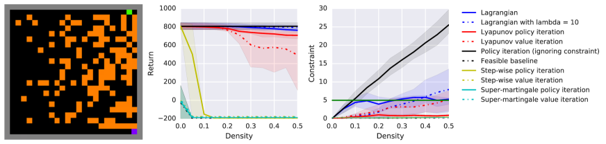
Figure 3: Results of various planning algorithms on the grid-world environment with obstacles (zoomed), with x-axis showing the obstacle density. From the leftmost column, the first figure illustrates the 2D planning domain example. The second and the third figure show the average return and the average cumulative constraint cost of the CMDP methods respectively. The fourth figure displays all the methods used in the experiment. The shaded regions indicate the $80\%$ confidence intervals. Clearly the safe DP algorithms compute policies that are safe and have good performance.

	Discrete obs, $d_{0}=5$	Discrete obs, $d_{0}=1$
Constraints                    Rewards

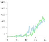
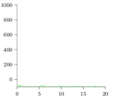
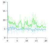
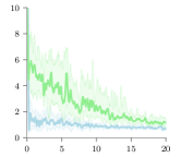
Figure 4: Results of using a saddle-point Lagrangian optimization for solving the grid-world environment with obstacles, with x-axis in thousands of episodes.

References

- [1] N. Abe, P. Melville, C. Pendus, C. Reddy, D. Jensen, V. Thomas, J. Bennett, G. Anderson, B. Cooley, M. Kowalczyk, et al. Optimizing debt collections using constrained reinforcement learning. In Proceedings of the 16th ACM SIGKDD international conference on Knowledge discovery and data mining, pages 75–84, 2010.
- [2] J. Achiam, D. Held, A. Tamar, and P. Abbeel. Constrained policy optimization. In International Conference of Machine Learning, 2017.
- [3] E. Altman. Constrained Markov decision processes, volume 7. CRC Press, 1999.
- [4] Eitan Altman. Constrained Markov decision processes with total cost criteria: Lagrangian approach and dual linear program. Mathematical methods of operations research, 48(3):387–417, 1998.
- [5] D. Amodei, C. Olah, J. Steinhardt, P. Christiano, J. Schulman, and D. Mané. Concrete problems in AI safety. arXiv preprint arXiv:1606.06565, 2016.
- [6] F. Berkenkamp, M. Turchetta, A. Schoellig, and A. Krause. Safe model-based reinforcement learning with stability guarantees. In Advances in Neural Information Processing Systems, pages 908–919, 2017.
- [7] D. Bertsekas. Dynamic programming and optimal control. Athena scientific Belmont, MA, 1995.
- [8] S. Boyd and L. Vandenberghe. Convex optimization. Cambridge university press, 2004.
- [9] M El Chamie, Y. Yu, and B. Açıkmeşe. Convex synthesis of randomized policies for controlled Markov chains with density safety upper bound constraints. In American Control Conference, pages 6290–6295, 2016.
- [10] Y. Chow, M. Pavone, B. Sadler, and S. Carpin. Trading safety versus performance: Rapid deployment of robotic swarms with robust performance constraints. Journal of Dynamic Systems, Measurement, and Control, 137(3), 2015.
- [11] Yinlam Chow, Mohammad Ghavamzadeh, Lucas Janson, and Marco Pavone. Risk-constrained reinforcement learning with percentile risk criteria. arXiv preprint arXiv:1512.01629, 2015.
- [12] G. Dalal, K. Dvijotham, M. Vecerik, T. Hester, C. Paduraru, and Y. Tassa. Safe exploration in continuous action spaces. arXiv preprint arXiv:1801.08757, 2018.
- [13] Z. Gábor and Z. Kalmár. Multi-criteria reinforcement learning. In International Conference of Machine Learning, 1998.
- [14] P. Geibel and F. Wysotzki. Risk-sensitive reinforcement learning applied to control under constraints. Journal of Artificial Intelligence Research, 24:81–108, 2005.
- [15] P. Glynn, A. Zeevi, et al. Bounding stationary expectations of markov processes. In Markov processes and related topics: a Festschrift for Thomas G. Kurtz, pages 195–214. Institute of Mathematical Statistics, 2008.
- [16] S. Gu, T. Lillicrap, I. Sutskever, and S. Levine. Continuous deep Q-learning with model-based acceleration. In International Conference on Machine Learning, pages 2829–2838, 2016.
- [17] S. Junges, N. Jansen, C. Dehnert, U. Topcu, and J. Katoen. Safety-constrained reinforcement learning for MDPs. In International Conference on Tools and Algorithms for the Construction and Analysis of Systems, pages 130–146, 2016.
- [18] S. Kakade and J. Langford. Approximately optimal approximate reinforcement learning. In International Conference on International Conference on Machine Learning, pages 267–274, 2002.
- [19] Hassan K Khalil. Noninear systems. Prentice-Hall, New Jersey, 2(5):5–1, 1996.
- [20] J. Lee, I. Panageas, G. Piliouras, M. Simchowitz, M. Jordan, and B. Recht. First-order methods almost always avoid saddle points. arXiv preprint arXiv:1710.07406, 2017.
- [21] J. Leike, M. Martic, V. Krakovna, P. Ortega, T. Everitt, A. Lefrancq, L. Orseau, and S. Legg. Ai safety gridworlds. arXiv preprint arXiv:1711.09883, 2017.
- [22] D. Luenberger, Y. Ye, et al. Linear and nonlinear programming, volume 2. Springer, 1984.
- [23] N. Mastronarde and M. van der Schaar. Fast reinforcement learning for energy-efficient wireless communication. IEEE Transactions on Signal Processing, 59(12):6262–6266, 2011.
- [24] V. Mnih, K. Kavukcuoglu, D. Silver, A. Graves, I. Antonoglou, D. Wierstra, and M. Riedmiller. Playing Atari with deep reinforcement learning. arXiv preprint arXiv:1312.5602, 2013.
- [25] T. Moldovan and P. Abbeel. Safe exploration in Markov decision processes. arXiv preprint arXiv:1205.4810, 2012.
- [26] H. Mossalam, Y. Assael, D. Roijers, and S. Whiteson. Multi-objective deep reinforcement learning. arXiv preprint arXiv:1610.02707, 2016.
- [27] M. Neely. Stochastic network optimization with application to communication and queueing systems. Synthesis Lectures on Communication Networks, 3(1):1–211, 2010.
- [28] G. Neu, A. Jonsson, and V. Gómez. A unified view of entropy-regularized markov decision processes. arXiv preprint arXiv:1705.07798, 2017.
- [29] M. Ono, M. Pavone, Y. Kuwata, and J. Balaram. Chance-constrained dynamic programming with application to risk-aware robotic space exploration. Autonomous Robots, 39(4):555–571, 2015.
- [30] T. Perkins and A. Barto. Lyapunov design for safe reinforcement learning. Journal of Machine Learning Research, 3:803–832, 2002.
- [31] K. Regan and C. Boutilier. Regret-based reward elicitation for Markov decision processes. In Proceedings of the Twenty-Fifth Conference on Uncertainty in Artificial Intelligence, pages 444–451, 2009.
- [32] D. Roijers, P. Vamplew, S. Whiteson, and R. Dazeley. A survey of multi-objective sequential decision-making. Journal of Artificial Intelligence Research, 48:67–113, 2013.
- [33] A. Rusu, S. Colmenarejo, C. Gulcehre, G. Desjardins, J. Kirkpatrick, R. Pascanu, V. Mnih, K. Kavukcuoglu, and R. Hadsell. Policy distillation. arXiv preprint arXiv:1511.06295, 2015.
- [34] T. Schaul, J. Quan, I. Antonoglou, and D. Silver. Prioritized experience replay. arXiv preprint arXiv:1511.05952, 2015.
- [35] Bruno Scherrer. Performance bounds for policy iteration and application to the game of Tetris. Journal of Machine Learning Research, 14(Apr):1181–1227, 2013.
- [36] M. Schmitt and L. Martignon. On the complexity of learning lexicographic strategies. Journal of Machine Learning Research, 7:55–83, 2006.
- [37] G. Shani, D. Heckerman, and R. Brafman. An MDP-based recommender system. Journal of Machine Learning Research, 6:1265–1295, 2005.
- [38] A. Tamar, D. Di Castro, and S. Mannor. Policy gradients with variance related risk criteria. In International Conference of Machine Learning, 2012.
- [39] H. van Hasselt. Double Q-learning. In Advances in Neural Information Processing Systems, pages 2613–2621, 2010.