Two-Stream Adaptive Graph Convolutional Networks for Skeleton-Based Action Recognition

Abstract

In skeleton-based action recognition, graph convolutional networks (GCNs), which model the human body skeletons as spatiotemporal graphs, have achieved remarkable performance. However, in existing GCN-based methods, the topology of the graph is set manually, and it is fixed over all layers and input samples. This may not be optimal for the hierarchical GCN and diverse samples in action recognition tasks. In addition, the second-order information (the lengths and directions of bones) of the skeleton data, which is naturally more informative and discriminative for action recognition, is rarely investigated in existing methods. In this work, we propose a novel two-stream adaptive graph convolutional network (2s-AGCN) for skeleton-based action recognition. The topology of the graph in our model can be either uniformly or individually learned by the BP algorithm in an end-to-end manner. This data-driven method increases the flexibility of the model for graph construction and brings more generality to adapt to various data samples. Moreover, a two-stream framework is proposed to model both the first-order and the second-order information simultaneously, which shows notable improvement for the recognition accuracy. Extensive experiments on the two large-scale datasets, NTU-RGBD and Kinetics-Skeleton, demonstrate that the performance of our model exceeds the state-of-the-art with a significant margin.

1 Introduction

Action recognition methods based on skeleton data have been widely investigated and attracted considerable attention due to their strong adaptability to the dynamic circumstance and complicated background [31, 8, 6, 27, 22, 29, 33, 19, 20, 21, 14, 13, 23, 18, 17, 32, 30, 34]. Conventional deep-learning-based methods manually structure the skeleton as a sequence of joint-coordinate vectors [6, 27, 22, 29, 33, 19, 20] or as a pseudo-image [21, 14, 13, 23, 18, 17], which is fed into RNNs or CNNs to generate the prediction. However, representing the skeleton data as a vector sequence or a 2D grid cannot fully express the dependency between correlated joints. The skeleton is naturally structured as a graph in a non-Euclidean space with the joints as vertexes and their natural connections in the human body as edges. The previous methods cannot exploit the graph structure of the skeleton data and are difficult to generalize to skeletons with arbitrary forms. Recently, graph convolutional networks (GCNs), which generalize convolution from image to graph, have been successfully adopted in many applications[16, 7, 25, 1, 9, 24, 15]. For the skeleton-based action recognition task, Yan et al. [32] first apply GCNs to model the skeleton data. They construct a spatial graph based on the natural connections of joints in the human body and add the temporal edges between corresponding joints in consecutive frames. A distance-based sampling function is proposed for constructing the graph convolutional layer, which is then employed as a basic module to build the final spatiotemporal graph convolutional network (ST-GCN).

However, there are three disadvantages for the process of the graph construction in ST-GCN [32]: (1) The skeleton graph employed in ST-GCN is heuristically predefined and represents only the physical structure of the human body. Thus it is not guaranteed to be optimal for the action recognition task. For example, the relationship between the two hands is important for recognizing classes such as “clapping” and “reading.” However, it is difficult for ST-GCN to capture the dependency between the two hands since they are located far away from each other in the predefined human-body-based graphs. (2) The structure of GCNs is hierarchical where different layers contain multilevel semantic information. However, the topology of the graph applied in ST-GCN is fixed over all the layers, which lacks the flexibility and capacity to model the multilevel semantic information contained in all of the layers; (3) One fixed graph structure may not be optimal for all the samples of different action classes. For classes such as “wiping face” and “touching head”, the connection between the hands and head should be stronger, but it is not true for some other classes, such as “jumping up” and “sitting down”. This fact suggests that the graph structure should be data dependent, which, however, is not supported in ST-GCN.

To solve the above problems, a novel adaptive graph convolutional network is proposed in this work. It parameterizes two types of graphs, the structure of which are trained and updated jointly with convolutional parameters of the model. One type is a global graph, which represents the common pattern for all the data. Another type is an individual graph, which represents the unique pattern for each data. Both of the two types of graphs are optimized individually for different layers, which can better fit the hierarchical structure of the model. This data-driven method increases the flexibility of the model for graph construction and brings more generality to adapt to various data samples.

Another notable problem in ST-GCN is that the feature vector attached to each vertex only contains 2D or 3D coordinates of the joints, which can be regarded as the first-order information of the skeleton data. However, the second-order information, which represents the feature of bones between two joints, is not exploited. Typically, the lengths and directions of bones are naturally more informative and discriminative for action recognition. In order to exploit the second-order information of the skeleton data, the lengths and directions of bones are formulated as a vector pointing from its source joint to its target joint. Similar to the first-order information, the vector is fed into an adaptive graph convolutional network to predict the action label. Moreover, a two-stream framework is proposed to fuse the first-order and second-order information to further improve the performance.

To verify the superiority of the proposed model, namely, the two-stream adaptive graph convolutional network (2s-AGCN), extensive experiments are performed on two large-scale datasets: NTU-RGBD [27] and Kinetics-Skeleton [12]. Our model achieves state-of-the-art performance on both of the datasets.

The main contributions of our work lie in three folds: (1) An adaptive graph convolutional network is proposed to adaptively learn the topology of the graph for different GCN layers and skeleton samples in an end-to-end manner, which can better suit the action recognition task and the hierarchical structure of the GCNs. (2) The second-order information of the skeleton data is explicitly formulated and combined with the first-order information using a two-stream framework, which brings notable improvement for the recognition performance. (3) On two large-scale datasets for skeleton-based action recognition, the proposed 2s-AGCN exceeds the state-of-the-art by a significant margin. The code will be released for future work and to facilitate communication.

2 Related work

2.1 Skeleton-based action recognition

Conventional methods for skeleton-based action recognition usually design handcrafted features to model the human body [31, 8]. However, the performance of these handcrafted-feature-based methods is barely satisfactory since it cannot consider all factors at the same time. With the development of deep learning, data-driven methods have become the mainstream methods, where the most widely used models are RNNs and CNNs. RNN-based methods usually model the skeleton data as a sequence of the coordinate vectors each represents a human body joint [6, 27, 22, 29, 33, 19, 20, 3]. CNN-based methods model the skeleton data as a pseudo-image based on the manually designed transformation rules [21, 14, 13, 23, 18, 17]. The CNN-based methods are generally more popular than RNN-based methods because the CNNs have better parallelizability and are easier to train than RNNs.

However, both RNNs and CNNs fail to fully represent the structure of the skeleton data because the skeleton data are naturally embedded in the form of graphs rather than a vector sequence or 2D grids. Recently, Yan et al. [32] propose a spatiotemporal graph convolutional network (ST-GCN) to directly model the skeleton data as the graph structure. It eliminates the need for designing handcrafted part assignment or traversal rules, thus achieves better performance than previous methods.

2.2 Graph convolutional neural networks

There have been many works on graph convolution, and the principle of constructing GCNs mainly follows two streams: spatial perspective and spectral perspective [28, 2, 11, 25, 1, 16, 7, 5, 9, 24, 15]. Spatial perspective methods directly perform the convolution filters on the graph vertexes and their neighbors, which are extracted and normalized based on manually designed rules [7, 25, 9, 24, 15]. In contrast to the spatial perspective methods, spectral perspective methods utilize the eigenvalues and eigenvectors of the graph Laplace matrices. These methods perform the graph convolution in the frequency domain with the help of the graph Fourier transform [28], which does not need to extract locally connected regions from graphs at each convolutional step [2, 11, 16, 5]. This work follows the spatial perspective methods.

3 Graph Convolutional Networks

3.1 Graph construction

The raw skeleton data in one frame are always provided as a sequence of vectors. Each vector represents the 2D or 3D coordinates of the corresponding human joint. A complete action contains multiple frames with different lengths for different samples. We employ a spatiotemporal graph to model the structured information among these joints along both the spatial and temporal dimensions. The structure of the graph follows the work of ST-GCN [32]. The left sketch in Fig. 1 presents an example of the constructed spatiotemporal skeleton graph, where the joints are represented as vertexes and their natural connections in the human body are represented as spatial edges (the orange lines in Fig. 1, left). For the temporal dimension, the corresponding joints between two adjacent frames are connected with temporal edges (the blue lines in Fig. 1, left). The coordinate vector of each joint is set as the attribute of the corresponding vertex.

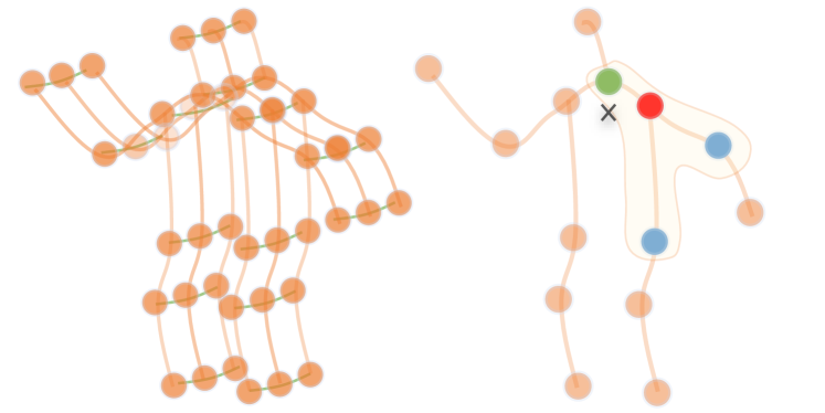
Figure 1: (a).Illustration of the spatiotemporal graph used in ST-GCN. (b).Illustration of the mapping strategy. Different colors denote different subsets.

3.2 Graph convolution

Given the graph defined above, multiple layers of spatiotemporal graph convolution operations are applied on the graph to extract the high-level features. The global average pooling layer and the $softmax$ classifier are then employed to predict the action categories based on the extracted features.

In the spatial dimension, the graph convolution operation on vertex $v_{i}$ is formulated as  [32]:

$$\mathit{f}_{out}(v_{i})=\sum_{v_{j}\in\mathcal{B}_{i}}\frac{1}{Z_{ij}}\mathit{f}_{in}(v_{j})\cdot{}w(l_{i}(v_{j}))$$ (1)

where $\mathit{f}$ denotes the feature map and $v$ denotes the vertex of the graph. $\mathcal{B}_{i}$ denotes the sampling area of the convolution for $v_{i}$, which is defined as the 1-distance neighbor vertexes ($v_{j}$) of the target vertex ($v_{i}$). $w$ is the weighting function similar to the original convolution operation, which provides a weight vector based on the given input. Note that the number of weight vectors of convolution is fixed, while the number of vertexes in $\mathcal{B}_{i}$ is varied. To map each vertex with a unique weight vector, a mapping function $l_{i}$ is designed specially in ST-GCN [32]. The right sketch in Fig. 1 shows this strategy, where $\times$ represents the center of gravity of the skeleton. $\mathcal{B}_{i}$ is the area enclosed by the curve. In detail, the strategy empirically sets the kernel size as 3 and naturally divides $\mathcal{B}_{i}$ into 3 subsets: $\mathcal{S}_{i1}$ is the vertex itself (the red circle in Fig. 1, right); $\mathcal{S}_{i2}$ is the centripetal subset, which contains the neighboring vertexes that are closer to the center of gravity (the green circle); $\mathcal{S}_{i3}$ is the centrifugal subset, which contains the neighboring vertexes that are farther from the center of gravity (the blue circle). $Z_{ij}$ denotes the cardinality of $\mathcal{S}_{ik}$ that contains $v_{j}$. It aims to balance the contribution of each subset.

3.3 Implementation

The implementation of the graph convolution in the spatial dimension is not straightforward. Concretely, the feature map of the network is actually a $C\times T\times N$ tensor, where $N$ denotes the number of vertexes, $T$ denotes the temporal length and $C$ denotes the number of channels. To implement the ST-GCN, Eq. 1 is transformed into

$$\mathbf{f}_{out}=\sum_{k}^{K_{v}}\mathbf{W}_{k}(\mathbf{f}_{in}{\mathbf{A}}_{k})\odot\mathbf{M}_{k}$$ (2)

where $K_{v}$ denotes the kernel size of the spatial dimension. With the partition strategy designed above, $K_{v}$ is set to $3$. $\mathbf{A}_{k}={\mathbf{\Lambda}}_{k}^{-\frac{1}{2}}{\mathbf{\bar{A}}}_{k}{\mathbf{\Lambda}}_{k}^{-\frac{1}{2}}$, where $\mathbf{\bar{A}}_{k}$ is similar to the $N\times N$ adjacency matrix, and its element $\mathbf{\bar{A}}_{k}^{ij}$ indicates whether the vertex $v_{j}$ is in the subset $S_{ik}$ of vertex $v_{i}$. It is used to extract the connected vertexes in a particular subset from $\mathbf{f}_{in}$ for the corresponding weight vector. $\mathbf{\Lambda}_{k}^{ii}=\sum_{j}(\mathbf{\bar{A}}_{k}^{ij})+\alpha$ is the normalized diagonal matrix. $\alpha$ is set to $0.001$ to avoid empty rows. $\mathbf{W}_{k}$ is the $C_{out}\times C_{in}\times 1\times 1$ weight vector of the $1\times 1$ convolution operation, which represents the weighting function $w$ in Eq. 1. $\mathbf{M}_{k}$ is an $N\times N$ attention map that indicates the importance of each vertex. $\odot$ denotes the dot product.

For the temporal dimension, since the number of neighbors for each vertex is fixed as $2$ (corresponding joints in the two consecutive frames), it is straightforward to perform the graph convolution similar to the classical convolution operation. Concretely, we perform a $K_{t}\times 1$ convolution on the output feature map calculated above, where $K_{t}$ is the kernel size of temporal dimension.

4 Two-stream adaptive graph convolutional network

In this section, we introduce the components of our proposed two-stream adaptive graph convolutional network (2s-AGCN) in detail.

4.1 Adaptive graph convolutional layer

The spatiotemporal graph convolution for the skeleton data described above is calculated based on a predefined graph, which may not be the best choice as explained in Sec. 1. To solve this problem, we propose an adaptive graph convolutional layer. It makes the topology of the graph optimized together with the other parameters of the network in an end-to-end learning manner. The graph is unique for different layers and samples, which greatly increases the flexibility of the model. Meanwhile, it is designed as a residual branch, which guarantees the stability of the original model.

In detail, according to Eq. 2, the topology of the graph is actually decided by the adjacency matrix and the mask, i.e., $\mathbf{A}_{k}$ and $\mathbf{M}_{k}$, respectively. $\mathbf{A}_{k}$ determines whether there are connections between two vertexes and $\mathbf{M}_{k}$ determines the strength of the connections. To make the graph structure adaptive, we change Eq. 2 into the following form:

$$\mathbf{f}_{out}=\sum_{k}^{K_{v}}\mathbf{W}_{k}\mathbf{f}_{in}({\mathbf{A}_{k}}+{\mathbf{B}_{k}}+{\mathbf{C}_{k}})$$ (3)

The main difference lies in the adjacency matrix of the graph, which is divided into three parts: $\mathbf{A}_{k}$, $\mathbf{B}_{k}$ and $\mathbf{C}_{k}$.

The first part ($\mathbf{A}_{k}$) is the same as the original normalized $N\times N$ adjacency matrix $\mathbf{A}_{k}$ in Eq. 2. It represents the physical structure of the human body.

The second part ($\mathbf{B}_{k}$) is also an $N\times N$ adjacency matrix. In contrast to $\mathbf{A}_{k}$, the elements of $\mathbf{B}_{k}$ are parameterized and optimized together with the other parameters in the training process. There are no constraints on the value of $\mathbf{B}_{k}$, which means that the graph is completely learned according to the training data. With this data-driven manner, the model can learn graphs that are fully targeted to the recognition task and more individualized for different information contained in different layers. Note that the element in the matrix can be an arbitrary value. It indicates not only the existence of the connections between two joints but also the strength of the connections. It can play the same role of the attention mechanism performed by $\mathbf{M}_{k}$ in Eq. 2However, the original attention matrix $\mathbf{M}_{k}$ is dot multiplied to $A_{k}$, which means that if one of the elements in $A_{k}$ is $0$, it will always be $0$ irrespective the value of $\mathbf{M}_{k}$. Thus, it cannot generate the new connections that not exist in the original physical graph. From this perspective, $\mathbf{B}_{k}$ is more flexible than $\mathbf{M}_{k}$.

The third part ($\mathbf{C}_{k}$) is a data-dependent graph which learn a unique graph for each sample. To determine whether there is a connection between two vertexes and how strong the connection is, we apply the normalized embedded Gaussian function to calculate the similarity of the two vertexes:

$$\mathit{f}(v_{i},v_{j})=\frac{e^{\theta(v_{i})^{T}\phi(v_{j})}}{\sum_{j=1}^{N}{e^{\theta(v_{i})^{T}\phi(v_{j})}}}$$ (4)

where $N$ is the total number of the vertexes. We use the dot product to measure the similarity of the two vertexes in an embedding space. In detail, given the input feature map $\mathbf{f_{in}}$ whose size is $C_{in}\times T\times N$, we first embed it into $C_{e}\times T\times N$ with two embedding functions, i.e., $\theta$ and $\phi$. Here, through extensive experiments, we choose one $1\times 1$ convolutional layer as the embedding function. The two embedded feature maps are rearranged and reshaped to an $N\times C_{e}T$ matrix and a $C_{e}T\times N$ matrix. They are then multiplied to obtain an $N\times N$ similarity matrix $\mathbf{C}_{k}$, whose element $\mathbf{C}_{k}^{ij}$ represents the similarity of vertex $v_{i}$ and vertex $v_{j}$. The value of the matrix is normalized to $0-1$, which is used as the soft edge of the two vertexes. Since the normalized Gaussian is equipped with a $softmax$ operation, we can calculate $\mathbf{C}_{k}$ based on Eq.4 as follows:

$$\mathbf{C}_{k}=softmax(\mathbf{f_{in}}^{T}\mathbf{W}^{T}_{\theta k}\mathbf{W}_{\phi k}\mathbf{f_{in}})$$ (5)

where $\mathbf{W_{\theta}}$ and $\mathbf{W_{\phi}}$ are the parameters of the embedding functions $\theta$ and $\phi$, respectively.

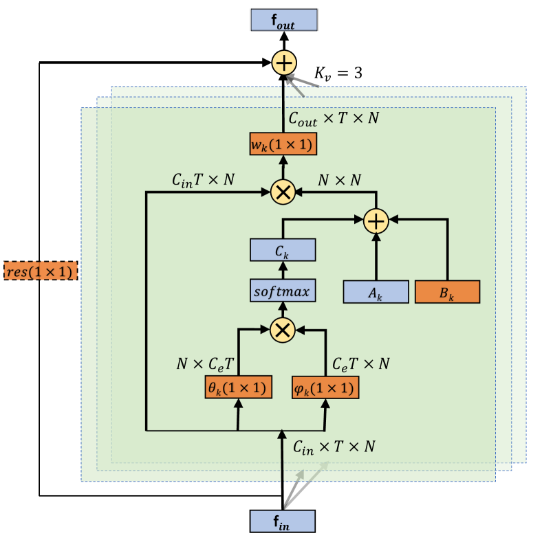
Figure 2: Illustration of the adaptive graph convolutional layer. There are a total of three types of graphs in each layer, i.e., $\mathbf{A}_{k}$, $\mathbf{B}_{k}$ and $\mathbf{C}_{k}$. The orange box indicates that the parameter is learnable. $(1\times 1)$ denotes the kernel size of convolution. $K_{v}$ denotes the number of subsets. $\oplus$ denotes the elementwise summation. $\otimes$ denotes the matirx multiplication. The residual box (dotted line) is only needed when $C_{in}$ is not the same as $C_{out}$.

Rather than directly replacing the original $\mathbf{A}_{k}$ with $\mathbf{B}_{k}$ or $\mathbf{C}_{k}$, we add them to it. The value of $\mathbf{B}_{k}$ and the parameters of $\theta$ and $\phi$ are initialized to $0$. In this way, it can strengthen the flexibility of the model without degrading the original performance.

The overall architecture of the adaptive graph convolution layer is shown in Fig. 2. Except for the $\mathbf{A}_{k}$, $\mathbf{B}_{k}$ and $\mathbf{C}_{k}$ introduced above, the kernel size of convolution ($K_{v}$) is set the same as before, i.e., 3. $w_{k}$ is the weighting function introduced in Eq. 1, whose parameter is $\mathbf{W}_{k}$ in Eq. 3. A residual connection, similar to [10], is added for each layer, which allows the layer to be inserted into any existing models without breaking its initial behavior. If the number of input channels is different than the number of output channels, a $1\times 1$ convolution (orange box with dashed line in Fig. 2) is inserted in the residual path to transform the input to match the output in the channel dimension.

4.2 Adaptive graph convolutional block

The convolution for the temporal dimension is the same as ST-GCN, i.e., performing the $K_{t}\times 1$ convolution on the $C\times T\times N$ feature maps. Both the spatial GCN and temporal GCN are followed by a batch normalization (BN) layer and a ReLU layer. As shown in Fig. 3, one basic block is the combination of one spatial GCN (Convs), one temporal GCN (Convt) and an additional dropout layer with the drop rate set as 0.5. To stabilize the training, a residual connection is added for each block.

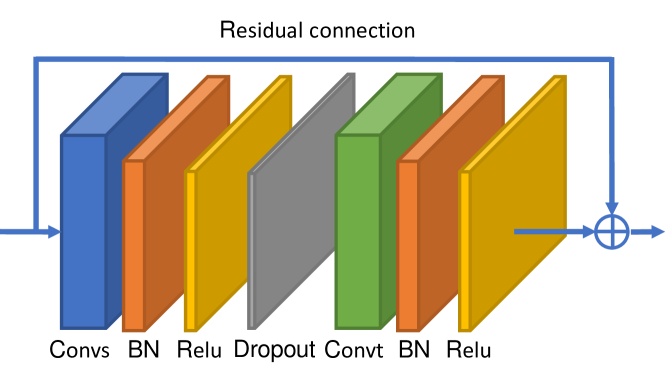
Figure 3: Illustration of the adaptive graph convolutional block. Convs represents the spatial GCN, and Convt represents the temporal GCN, both of which are followed by a BN layer and a ReLU layer. Moreover, a residual connection is added for each block.

4.3 Adaptive graph convolutional network

The adaptive graph convolutional network (AGCN) is the stack of these basic blocks, as shown in Fig. 4. There are a total of $9$ blocks. The numbers of output channels for each block are $64$, $64$, $64$, $128$, $128$, $128$, $256$, $256$ and $256$. A data BN layer is added at the beginning to normalize the input data. A global average pooling layer is performed at the end to pool feature maps of different samples to the same size. The final output is sent to a $softmax$ classifier to obtain the prediction.

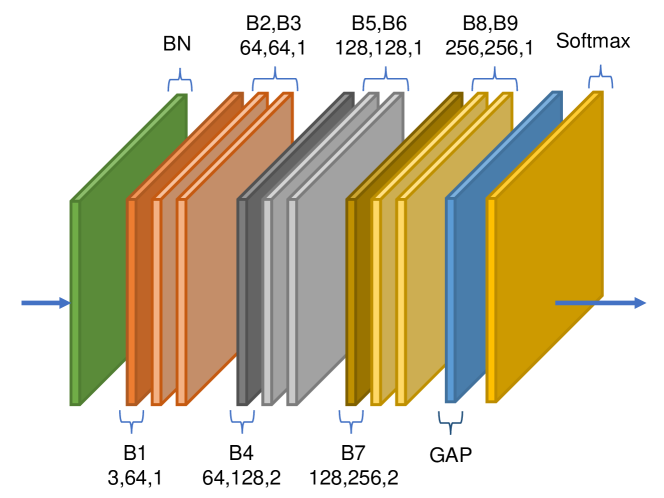
Figure 4: Illustration of the AGCN. There are a total of $9$ blocks (B1-B9). The three numbers of each block represent the number of input channels, the number of output channels and the stride, respectively. GAP represents the global average pooling layer.

4.4 Two-stream networks

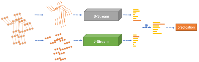
Figure 5: Illustration of the overall architecture of the 2s-AGCN. The scores of two streams are added to obtain the final prediction.

As introduced in Sec. 1, the second-order information, i.e., the bone information, is also important for skeleton-based action recognition but is neglected in previous works. In this paper, we propose explicitly modeling the second-order information, namely, the bone information, with a two-stream framework to enhance the recognition.

In particular, since each bone is bound with two joints, we define that the joint close to the center of gravity of the skeleton is the source joint and the joint far away from the center of gravity is the target joint. Each bone is represented as a vector pointing to its target joint from its source joint, which contains not only the length information, but also the direction information. For example, given a bone with its source joint $\mathbf{v_{1}}=(x_{1},y_{1},z_{1})$ and its target joint $\mathbf{v_{2}}=(x_{2},y_{2},z_{2})$, the vector of the bone is calculated as $\mathbf{e_{v_{1},v_{2}}}=(x_{2}-x_{1},y_{2}-y_{1},z_{2}-z_{1})$.

Since the graph of the skeleton data have no cycles, each bone can be assigned with a unique target joint. The number of joints is one more than the number of bones because the central joint is not assigned to any bones. To simplify the design of the network, we add an empty bone with its value as $0$ to the central joint. In this way, both the graph and the network of bones can be designed the same as that of joints because each bone can be bound with a unique joint. We use J-stream and B-stream to represent the networks of joints and bones, respectively. The overall architecture (2s-AGCN) is shown in Fig. 5. Given a sample, we first calculate the data of bones based on the data of joints. Then, the joint data and bone data are fed into the J-stream and B-stream, respectively. Finally, the $softmax$ scores of the two streams are added to obtain the fused score and predict the action label.

5 Experiments

To perform a head-to-head comparison with ST-GCN, our experiments are conducted on the same two large-scale action recognition datasets: NTU-RGBD [27] and Kinetics-Skeleton [12, 32]. First, since the NTU-RGBD dataset is smaller than the Kinetics-Skeleton dataset, we perform exhaustive ablation studies on it to examine the contributions of the proposed model components based on the recognition performance. Then, the final model is evaluated on both of the datasets to verify the generality and is compared with the other state-of-the-art approaches. The definitions of joints and their natural connections in the two datasets are shown in Fig. 6.

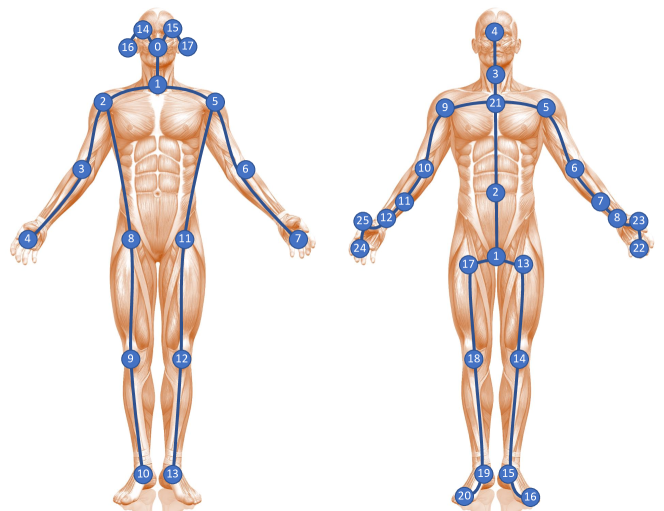
Figure 6: The left sketch shows the joint label of the Kinetics-Skeleton dataset and the right sketch shows the joint label of the NTU-RGBD dataset.

5.1 Datasets

NTU-RGBD: NTU-RGBD [27] is currently the largest and most widely used in-door-captured action recognition dataset, which contains 56,000 action clips in 60 action classes. The clips are performed by 40 volunteers in different age groups ranging from 10 to 35. Each action is captured by 3 cameras at the same height but from different horizontal angles: $-45^{\circ},0^{\circ},45^{\circ}$. This dataset provides 3D joint locations of each frame detected by Kinect depth sensors. There are 25 joints for each subject in the skeleton sequences, while each video has no more than 2 subjects. The original paper [27] of the dataset recommends two benchmarks: 1). Cross-subject (X-Sub): the dataset in this benchmark is divided into a training set (40,320 videos) and a validation set (16,560 videos), where the actors in the two subsets are different. 2).Cross-view (X-View): the training set in this benchmark contains 37,920 videos that are captured by cameras 2 and 3, and the validation set contains 18,960 videos that are captured by camera 1. We follow this convention and report the top-1 accuracy on both benchmarks.

Kinetics-Skeleton: Kinetics [12] is a large-scale human action dataset that contains 300,000 videos clips in 400 classes. The video clips are sourced from YouTube videos and have a great variety. It only provides raw video clips without skeleton data. [32] estimate the locations of 18 joints on every frame of the clips using the publicly available OpenPose toolbox [4]. Two peoples are selected for multiperson clips based on the average joint confidence. We use their released data (Kinetics-Skeleton) to evaluate our model. The dataset is divided into a training set (240,000 clips) and a validation set (20,000 clips). Following the evaluation method in [32], we train the models on the training set and report the top-1 and top-5 accuracies on the validation set.

5.2 Training details

All experiments are conducted on the PyTorch deep learning framework [26]. Stochastic gradient descent (SGD) with Nesterov momentum ($0.9$) is applied as the optimization strategy. The batch size is $64$. Cross-entropy is selected as the loss function to backpropagate gradients. The weight decay is set to $0.0001$.

For the NTU-RGBD dataset, there are at most two people in each sample of the dataset. If the number of bodies in the sample is less than 2, we pad the second body with 0. The max number of frames in each sample is 300. For samples with less than 300 frames, we repeat the samples until it reaches 300 frames. The learning rate is set as $0.1$ and is divided by $10$ at the $30_{th}$ epoch and $40_{th}$ epoch. The training process is ended at the $50_{th}$ epoch.

For the Kinetics-Skeleton dataset, the size of the input tensor of Kinetics is set the same as [32], which contains 150 frames with 2 bodies in each frame. We perform the same data-augmentation methods as in [32]. In detail, we randomly choose 150 frames from the input skeleton sequence and slightly disturb the joint coordinates with randomly chosen rotations and translations. The learning rate is also set as $0.1$ and is divided by $10$ at the $45_{th}$ epoch and $55_{th}$ epoch. The training process is ended at the $65_{th}$ epoch.

5.3 Ablation Study

We examine the effectiveness of the proposed components in two-stream adaptive graph convolutional network (2s-AGCN) in this section with the X-View benchmark on the NTU-RGBD dataset. The original performance of ST-GCN on the NTU-RGBD dataset is $88.3\%$. By using the rearranged learning-rate scheduler and the specially designed data preprocessing methods, it is improved to $92.7\%$, which is used as the baseline in the experiments. The detail is introduced in the supplementary material.

5.3.1 Adaptive graph convolutional block.

As introduced in Section 4.1, there are $3$ types of graphs in the adaptive graph convolutional block, i.e., $A$, $B$ and $C$. We manually delete one of the graphs and show their performance in Tab. 1. This table shows that adaptively learning the graph is beneficial for action recognition and that deleting any one of the three graphs will harm the performance. With all three graphs added together, the model obtains the best performance. We also test the importance of $\mathbf{M}$ used in the original ST-GCN. The result shows that given each connection, a weight parameter is important, which also proves the importance of the adaptive graph structure.

Methods	Accuracy ($\%$)
ST-GCN	92.7
ST-GCN wo/M	91.1
AGCN wo/A	93.4
AGCN wo/B	93.3
AGCN wo/C	93.4
AGCN	93.7

Table 1: Comparisons of the validation accuracy when adding adaptive graph convolutional block with or without $A$, $B$ and $C$. wo/X means deleting the X module.

5.3.2 Visualization of the learned graphs

Fig. 7 shows an example of the adjacency matrix learned by our model for the second subset. The gray scale of each element in the matrix represents the strength of the connection. The left is the original adjacency matrix for the second subset employed in ST-GCN, and the right is an example of the corresponding adaptive adjacency matrix learned by our model. It is clear that the learned structure of the graph is more flexible and not constrained to the physical connections of the human body.

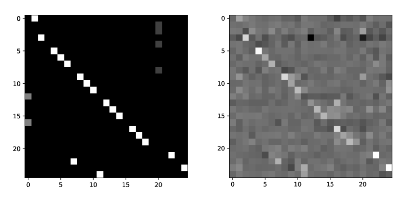
Figure 7: Example of the learned adjacency matrix. The left matrix is the original adjacency matrix for the second subset in the NTU-RGBD dataset. The right matrix is an example of the corresponding adaptive adjacency matrix learned by our model.

Fig. 8 is a visualization of the skeleton graph for different layers of one sample (from left to right is the $3_{rd}$, $5_{th}$ and $7_{th}$ layers in Fig. 4, respectively). The skeletons are plotted based on the physical connections of the human body. Each circle represents one joint, and its size represents the strength of the connection between the current joint and the $25_{th}$ joint in the learned adaptive graph of our model. It shows that a traditional physical connection of the human body is not the best choice for the action recognition task, and different layers need graphs with different topology structures. The skeleton graph in the $3_{rd}$ layer pays more attention to the adjacent joints in the physical graph. This result is intuitive since the lower layer only contains the low-level feature, while the global information cannot be observed. For the $5_{th}$ layer, more joints along the same arm are strongly connected. For the $7_{th}$ layer, the left hand and the right hand show a stronger connection, although they are far away from each other in the physical structure of the human body. We argue that a higher layer contains higher-level information. Hence, the graph is more relevant to the final classification task.

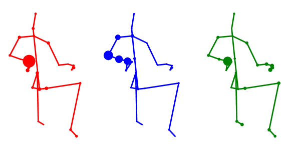
Figure 8: Visualization of the graphs for different layers.

Fig. 9 shows a similar visualization of Fig. 8 but for different samples. The learned adjacency matrix is extracted from the second subset of the $5_{th}$ layer in the model (Fig. 4). It shows that the graph structures learned by our model for different samples are also different, even for the same convolutional subset and the same layer. It verified our point of view that different samples need different topologies of the graph, and a data-driven graph structure is better than a fixed one.

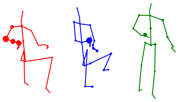
Figure 9: Visualization of the graphs for different samples.

5.3.3 Two-stream framework

Another important improvement is the utilization of second-order information. Here, we compare the performance of using each type of input data alone, shown as Js-AGCN and Bs-AGCN in Tab. 2, and the performance when combining them as described in Section 4.4, shown as 2s-AGCN in Tab. 2. Clearly, the two-stream method outperforms the one-stream-based methods.

Methods	Accuracy ($\%$)
Js-AGCN	93.7
Bs-AGCN	93.2
2s-AGCN	95.1

Table 2: Comparisons of the validation accuracy with different input modalities.

5.4 Comparison with the state-of-the-art

We compare the final model with the state-of-the-art skeleton-based action recognition methods on both the NTU-RGBD dataset and Kinetics-Skeleton dataset. The results of these two comparisons are shown in Tab 3 and Tab 4, respectively. The methods used for comparison include the handcraft-feature-based methods [31, 8], RNN-based methods [6, 27, 22, 29, 33, 19, 20], CNN-based methods [21, 14, 13, 23, 18, 17] and GCN-based methods [32, 30]. Our model achieves state-of-the-art performance with a large margin on both of the datasets, which verifies the superiority of our model.

Methods	X-Sub (%)	X-View (%)
Lie Group [31]	50.1	82.8
HBRNN [6]	59.1	64.0
Deep LSTM [27]	60.7	67.3
ST-LSTM [22]	69.2	77.7
STA-LSTM [29]	73.4	81.2
VA-LSTM [33]	79.2	87.7
ARRN-LSTM [19]	80.7	88.8
Ind-RNN [20]	81.8	88.0
Two-Stream 3DCNN [21]	66.8	72.6
TCN [14]	74.3	83.1
Clips+CNN+MTLN [13]	79.6	84.8
Synthesized CNN [23]	80.0	87.2
CNN+Motion+Trans [18]	83.2	89.3
3scale ResNet152 [17]	85.0	92.3
ST-GCN [32]	81.5	88.3
DPRL+GCNN [30]	83.5	89.8
2s-AGCN (ours)	88.5	95.1

Table 3: Comparisons of the validation accuracy with state-of-the-art methods on the NTU-RGBD dataset.

Methods	Top-1 (%)	Top-5 (%)
Feature Enc. [8]	14.9	25.8
Deep LSTM [27]	16.4	35.3
TCN [14]	20.3	40.0
ST-GCN [32]	30.7	52.8
Js-AGCN (ours)	35.1	57.1
Bs-AGCN (ours)	33.3	55.7
2s-AGCN (ours)	36.1	58.7

Table 4: Comparisons of the validation accuracy with state-of-the-art methods on the Kinetics-Skeleton dataset.

5.5 Conclusion

In this work, we propose a novel adaptive graph convolutional neural network (2s-AGCN) for skeleton-based action recognition. It parameterizes the graph structure of the skeleton data and embeds it into the network to be jointly learned and updated with the model. This data-driven approach increases the flexibility of the graph convolutional network and is more suitable for the action recognition task. Furthermore, the traditional methods always ignore or underestimate the importance of second-order information of skeleton data, i.e., the bone information. In this work, we propose a two-stream framework to explicitly employ this type of information, which further enhances the performance. The final model is evaluated on two large-scale action recognition datasets, NTU-RGBD and Kinetics, and it achieves the state-of-the-art performance on both of them.

References

- [1] James Atwood and Don Towsley. Diffusion-convolutional neural networks. In Advances in Neural Information Processing Systems, pages 1993–2001, 2016.
- [2] Joan Bruna, Wojciech Zaremba, Arthur Szlam, and Yann LeCun. Spectral Networks and Locally Connected Networks on Graphs. In ICLR, 2014.
- [3] C. Cao, C. Lan, Y. Zhang, W. Zeng, H. Lu, and Y. Zhang. Skeleton-Based Action Recognition with Gated Convolutional Neural Networks. IEEE Transactions on Circuits and Systems for Video Technology, pages 1–1, 2018.
- [4] Zhe Cao, Tomas Simon, Shih-En Wei, and Yaser Sheikh. Realtime multi-person 2d pose estimation using part affinity fields. In CVPR, 2017.
- [5] Michaël Defferrard, Xavier Bresson, and Pierre Vandergheynst. Convolutional Neural Networks on Graphs with Fast Localized Spectral Filtering. In D. D. Lee, M. Sugiyama, U. V. Luxburg, I. Guyon, and R. Garnett, editors, Advances in Neural Information Processing Systems 29, pages 3844–3852. Curran Associates, Inc., 2016.
- [6] Yong Du, Wei Wang, and Liang Wang. Hierarchical recurrent neural network for skeleton based action recognition. In Proceedings of the IEEE conference on computer vision and pattern recognition, pages 1110–1118, 2015.
- [7] David K Duvenaud, Dougal Maclaurin, Jorge Iparraguirre, Rafael Bombarell, Timothy Hirzel, Alan Aspuru-Guzik, and Ryan P Adams. Convolutional Networks on Graphs for Learning Molecular Fingerprints. In C. Cortes, N. D. Lawrence, D. D. Lee, M. Sugiyama, and R. Garnett, editors, Advances in Neural Information Processing Systems 28, pages 2224–2232. Curran Associates, Inc., 2015.
- [8] Basura Fernando, Efstratios Gavves, Jose M. Oramas, Amir Ghodrati, and Tinne Tuytelaars. Modeling video evolution for action recognition. In Proceedings of the IEEE Conference on Computer Vision and Pattern Recognition, pages 5378–5387, 2015.
- [9] Will Hamilton, Zhitao Ying, and Jure Leskovec. Inductive representation learning on large graphs. In Advances in Neural Information Processing Systems, pages 1025–1035, 2017.
- [10] Kaiming He, Xiangyu Zhang, Shaoqing Ren, and Jian Sun. Deep Residual Learning for Image Recognition. In The IEEE Conference on Computer Vision and Pattern Recognition (CVPR), June 2016.
- [11] Mikael Henaff, Joan Bruna, and Yann LeCun. Deep convolutional networks on graph-structured data. arXiv preprint arXiv:1506.05163, 2015.
- [12] Will Kay, Joao Carreira, Karen Simonyan, Brian Zhang, Chloe Hillier, Sudheendra Vijayanarasimhan, Fabio Viola, Tim Green, Trevor Back, Paul Natsev, and others. The Kinetics Human Action Video Dataset. arXiv preprint arXiv:1705.06950, 2017.
- [13] Qiuhong Ke, Mohammed Bennamoun, Senjian An, Ferdous Ahmed Sohel, and Farid Boussaïd. A New Representation of Skeleton Sequences for 3d Action Recognition. 2017 IEEE Conference on Computer Vision and Pattern Recognition (CVPR), pages 4570–4579, 2017.
- [14] Tae Soo Kim and Austin Reiter. Interpretable 3d human action analysis with temporal convolutional networks. In Computer Vision and Pattern Recognition Workshops (CVPRW), 2017 IEEE Conference on, pages 1623–1631, 2017.
- [15] Thomas Kipf, Ethan Fetaya, Kuan-Chieh Wang, Max Welling, and Richard Zemel. Neural relational inference for interacting systems. In International Conference on Machine Learning (ICML), 2018.
- [16] Thomas N. Kipf and Max Welling. Semi-Supervised Classification with Graph Convolutional Networks. arXiv preprint arXiv:1609.02907, Sept. 2016.
- [17] Bo Li, Yuchao Dai, Xuelian Cheng, Huahui Chen, Yi Lin, and Mingyi He. Skeleton based action recognition using translation-scale invariant image mapping and multi-scale deep CNN. In Multimedia & Expo Workshops (ICMEW), 2017 IEEE International Conference on, pages 601–604. IEEE, 2017.
- [18] Chao Li, Qiaoyong Zhong, Di Xie, and Shiliang Pu. Skeleton-based action recognition with convolutional neural networks. In Multimedia & Expo Workshops (ICMEW), 2017 IEEE International Conference on, pages 597–600. IEEE, 2017.
- [19] Lin Li, Wu Zheng, Zhaoxiang Zhang, Yan Huang, and Liang Wang. Skeleton-Based Relational Modeling for Action Recognition. arXiv:1805.02556 [cs], 2018.
- [20] Shuai Li, Wanqing Li, Chris Cook, Ce Zhu, and Yanbo Gao. Independently recurrent neural network (indrnn): Building A longer and deeper RNN. In Proceedings of the IEEE Conference on Computer Vision and Pattern Recognition, pages 5457–5466, 2018.
- [21] Hong Liu, Juanhui Tu, and Mengyuan Liu. Two-Stream 3d Convolutional Neural Network for Skeleton-Based Action Recognition. arXiv:1705.08106 [cs], May 2017.
- [22] Jun Liu, Amir Shahroudy, Dong Xu, and Gang Wang. Spatio-Temporal LSTM with Trust Gates for 3d Human Action Recognition. In Computer Vision – ECCV 2016, volume 9907, pages 816–833. Springer International Publishing, Cham, 2016.
- [23] Mengyuan Liu, Hong Liu, and Chen Chen. Enhanced skeleton visualization for view invariant human action recognition. Pattern Recognition, 68:346–362, 2017.
- [24] Federico Monti, Davide Boscaini, Jonathan Masci, Emanuele Rodola, Jan Svoboda, and Michael M. Bronstein. Geometric deep learning on graphs and manifolds using mixture model CNNs. In Proc. CVPR, volume 1, page 3, 2017.
- [25] Mathias Niepert, Mohamed Ahmed, and Konstantin Kutzkov. Learning convolutional neural networks for graphs. In International conference on machine learning, pages 2014–2023, 2016.
- [26] Adam Paszke, Sam Gross, Soumith Chintala, Gregory Chanan, Edward Yang, Zachary DeVito, Zeming Lin, Alban Desmaison, Luca Antiga, and Adam Lerer. Automatic differentiation in PyTorch. In NIPS-W, 2017.
- [27] Amir Shahroudy, Jun Liu, Tian-Tsong Ng, and Gang Wang. NTU RGB+D: A Large Scale Dataset for 3d Human Activity Analysis. In The IEEE Conference on Computer Vision and Pattern Recognition (CVPR), 2016.
- [28] David I Shuman, Sunil K Narang, Pascal Frossard, Antonio Ortega, and Pierre Vandergheynst. The emerging field of signal processing on graphs: Extending high-dimensional data analysis to networks and other irregular domains. IEEE Signal Processing Magazine, 30(3):83–98, 2013.
- [29] Sijie Song, Cuiling Lan, Junliang Xing, Wenjun Zeng, and Jiaying Liu. An End-to-End Spatio-Temporal Attention Model for Human Action Recognition from Skeleton Data. In AAAI, volume 1, pages 4263–4270, 2017.
- [30] Yansong Tang, Yi Tian, Jiwen Lu, Peiyang Li, and Jie Zhou. Deep Progressive Reinforcement Learning for Skeleton-Based Action Recognition. In The IEEE Conference on Computer Vision and Pattern Recognition (CVPR), 2018.
- [31] Raviteja Vemulapalli, Felipe Arrate, and Rama Chellappa. Human action recognition by representing 3d skeletons as points in a lie group. In Proceedings of the IEEE conference on computer vision and pattern recognition, pages 588–595, 2014.
- [32] Sijie Yan, Yuanjun Xiong, and Dahua Lin. Spatial Temporal Graph Convolutional Networks for Skeleton-Based Action Recognition. In AAAI, 2018.
- [33] Pengfei Zhang, Cuiling Lan, Junliang Xing, Wenjun Zeng, Jianru Xue, and Nanning Zheng. View Adaptive Recurrent Neural Networks for High Performance Human Action Recognition From Skeleton Data. In Proceedings of the IEEE Conference on Computer Vision and Pattern Recognition, pages 2117–2126, 2017.
- [34] Yifan Zhang, Congqi Cao, Jian Cheng, and Hanqing Lu. EgoGesture: A New Dataset and Benchmark for Egocentric Hand Gesture Recognition. IEEE Transactions on Multimedia, pages 1–1, 2018.